GNMR: A provable one-line algorithm for low rank matrix recovery

Abstract

Low rank matrix recovery problems appear in a broad range of applications. In this work we present GNMR — an extremely simple iterative algorithm for low rank matrix recovery, based on a Gauss-Newton linearization. On the theoretical front, we derive recovery guarantees for GNMR in both matrix sensing and matrix completion settings. Some of these results improve upon the best currently known for other methods. A key property of GNMR is that it implicitly keeps the factor matrices approximately balanced throughout its iterations. On the empirical front, we show that for matrix completion with uniform sampling, GNMR performs better than several popular methods, especially when given very few observations close to the information limit.

1 Introduction

Low rank matrices play a fundamental role in a broad range of applications in multiple scientific fields. In many cases the matrix is not fully observed, and yet it is often possible to recover it due to its assumed low rank structure. In this paper we propose a novel method, denoted GNMR, to tackle this class of problems. GNMR (Gauss-Newton Matrix Recovery) is a very simple iterative method with state-of-the-art performance, for which we also derive strong theoretical recovery guarantees. As detailed below, some of our guarantees improve upon the best currently available for other methods.

Concretely, consider the problem of recovering a matrix $X^{*}\in\mathbb{R}^{n_{1}\times n_{2}}$ of known rank $r$ from a set of $m$ linear measurements $b\equiv\mathcal{A}(X^{*})+\xi$ where $\mathcal{A}:\mathbb{R}^{n_{1}\times n_{2}}\to\mathbb{R}^{m}$ is a sensing operator and $\xi\in\mathbb{R}^{m}$ is additive error. Formally, the goal is to solve the optimization problem

$$\min_{X}\,f(X)\quad\text{s.t. rank(}X)\leq r$$ (1)

where

$$f(X)=\|\mathcal{A}(X)-b\|_{2}^{2}.$$ (2)

Two common cases of Eq. 1 are matrix sensing and matrix completion. These and related problems appear in a wide variety of applications, including collaborative filtering, manifold learning, quantum computing, image processing and computer vision, see [BF05, CP10, DR16, CL19, CLC19] and references therein. In the matrix sensing problem, for well-posedness of Eq. 1 for any rank-$r$ matrix $X^{*}$, the sensing operator $\mathcal{A}$ is required to satisfy a suitable RIP (Restricted Isometry Property) [Can08, RFP10]. In the matrix completion problem, the operator $\mathcal{A}$ extracts $m$ entries of the underlying matrix, $X^{*}_{i,j}$ for $(i,j)\in\Omega$ where $\Omega\subseteq[n_{1}]\times[n_{2}]$ is of size $m$. In this case, $\mathcal{A}$ does not satisfy an RIP. However, if $\Omega$ is sampled uniformly at random with large enough cardinality $|\Omega|$ and $X^{*}$ is incoherent, then with high probability $X^{*}$ is the unique solution of Eq. 1; see [CP10, CT10, Gro11, SC10, PABN16] for more details.

In general, matrix recovery problems of the form of Eq. 1 are NP-hard. Yet, due to their importance, various methods to find approximate solutions were developed. Most of them can be assigned to one of two classes. The first consists of algorithms which optimize over the full $n_{1}\times n_{2}$ matrix. Some methods in this class replace the rank-$r$ constraint by a suitable matrix penalty that promotes a low rank solution. One popular choice is the nuclear norm, which leads to a convex semi-definite program [FHB⁺01]. Nuclear norm minimization enjoys strong theoretical guarantees [CR09, CT10, Rec11], but in general is computationally slow. Hence, several works developed fast optimization methods, see [RS05, JY09, CCS10, MHT10, TY10, FRW11, MGC11, AKKS12] and references therein. Another matrix penalty that promotes low rank solutions is the non-convex Schatten $p$-norm with $p<1$ [MS12, KS18].

The other class consists of methods that explicitly enforce the rank-$r$ constraint in Eq. 1. For example, hard thresholding methods keep at each iteration only the top $r$ principal components [JMD10, TW13, BTW15, KC14]. Other methods in this class employ the decomposition $X=UV^{\top}$ with $U\in\mathbb{R}^{n_{1}\times r}$, $V\in\mathbb{R}^{n_{2}\times r}$. The matrix recovery objective Eq. 1 then reads

$$\min_{U,V}f\left(UV^{\top}\right).$$ (3)

As the factorized problem Eq. 3 involves only $(n_{1}+n_{2})r$ variables, these methods are in general more scalable and can cope with larger matrices. One approach to solve Eq. 3 is alternating minimization [HH09, Kes12, WYZ12, JNS13]. Another approach is gradient descent, either on the Euclidean manifold [SL16, TBS⁺16] or on other Riemannian manifolds [KMO10, NS12, Van13, MS14, MMBS14, BA15]. Some of the above works also derived recovery guarantees for these methods. For additional guarantees, see [Har14, JN15, YPCC16, ZL16, WCCL16, MWCC19, CLL20, MLC21, TMC21a] and references therein.

Most matrix completion methods proposed thus far suffer from two limitations: they may fail to recover the underlying matrix $X^{*}$ if it is even mildly ill-conditioned, or if the number of observed entries $m$ is relatively small [TW13, BNZ21, KV20]. This may pose a significant drawback in practical applications. Two recent algorithms that are relatively scalable and perform well with ill-conditioning and few observations are R2RILS [BNZ21] and MatrixIRLS [KV20, KV21]. However, only limited recovery guarantees are available for them. This raises the following question: is there an algorithm that is both computationally efficient, succeeds on ill-conditioned matrices with few measurements, and enjoys strong theoretical recovery guarantees?

In this work we make a step towards answering this question. In Section 2 we present a novel iterative algorithm which both empirically outperforms existing methods (including R2RILS and MatrixIRLS) in the task of recovering ill-conditioned matrices from few observations, and for which we are able to derive strong recovery guarantees due to its remarkable simplicity. Our proposed factorization-based algorithm, named GNMR, is based on the classical Gauss-Newton method. At each iteration, GNMR solves a simple least squares problem obtained by a linearization of the factorized objective Eq. 3. The resulting least squares problem can be solved efficiently by standard solvers.

On the theoretical front, in Section 3 we present recovery guarantees for GNMR in both the matrix sensing and matrix completion settings. In matrix sensing, we prove that starting from a sufficiently accurate initial estimate, GNMR recovers the underlying matrix with quadratic rate under the minimal RIP assumptions on the sensing operator $\mathcal{A}$, see Theorem 3.3. To the best of our knowledge, this guarantee is among the sharpest currently available for any recovery algorithm. Moreover, we prove that in matrix sensing, a slightly modified variant of GNMR is stable against arbitrary additive error of bounded norm. Importantly, this type of error also captures the practical setting of approximately low rank, where $X^{*}$ has $r$ large singular values and the remaining ones are much smaller yet nonzero. Next, in Section 3.2 we analyze GNMR in the matrix completion setting. Here we follow the standard approach in the literature, whereby to derive recovery guarantees for factorization-based methods, suitable regularization terms are added to the respective algorithm, see for example [KMO10, SL16]. In Theorem 3.5 we prove that given a sufficiently accurate initialization, a regularized variant of GNMR recovers the target matrix at a linear rate under the weakest known assumptions for non-convex optimization methods. In addition, in Theorem 3.7 we prove that near the global optimum, the convergence rate of GNMR is quadratic.

Our proof technique builds upon recent works which derived guarantees for gradient descent algorithms [KMO10, TBS⁺16, SL16, ZL16, YPCC16, MLC21]. However, as GNMR is markedly different, deriving recovery guarantees for it required several non-trivial modifications. In particular, while the iterates of gradient descent have a simple explicit formula, GNMR solves a degenerate least squares problem. In our analysis, we exploit this degeneracy in our favor, and show that by choosing the minimal norm solution the iterates of GNMR enjoy some desirable properties such as implicit balance regularization, see Section 3.5 for more details. In the course of our proofs, we extended and improved several technical results from previous works, including [TBS⁺16, Lemma 5.14], [MLC21, Lemma 1] and [SL16, Claim 3.1]. Specifically, in Theorem 3.9 we present a novel RIP-like guarantee for matrix completion which is in several aspects sharper than [SL16, Claim 3.1], especially in terms of the required number of observations. These improvements may be of independent interest, e.g. for proving recovery guarantees of other algorithms.

On the empirical front, in Section 5 we present several simulations with ill-conditioned matrices and few observed entries chosen uniformly at random. We show that GNMR improves upon the state of the art in these settings, outperforming several popular algorithms. In particular, GNMR is able to successfully recover matrices from very few observations close to the information limit, where all other compared methods fail.

Notation. The $i$’th largest singular value of a matrix $X$ is denoted by $\sigma_{i}(X)$. The condition number of a rank-$r$ matrix is denoted by $\kappa=\sigma_{1}/\sigma_{r}$. Denote the Euclidean norm of a vector $x$ by $\|x\|$. Denote the trace of a matrix $A$ by $\operatorname{Tr}(A)$, its operator norm (a.k.a. spectral norm) by $\|A\|_{2}$, its Frobenius norm by $\|A\|_{F}$, its $i$’th row by $A^{(i)}$, and its largest row norm by $\|A\|_{2,\infty}\equiv\max_{i}\|A^{(i)}\|$. The transpose of the inverse of $A$ is denoted by $A^{-\top}\equiv(A^{-1})^{\top}$. In the matrix completion problem, the fraction of observed entries is denoted by $p={|\Omega|}/{(n_{1}n_{2})}={m}/{(n_{1}n_{2})}$. The sampling operator $\mathcal{P}_{\Omega}$ extracts the entries of a matrix according to $\Omega$, such that $\mathcal{P}_{\Omega}(X)$ is a vector of size $m$ with entries $X_{ij}$ for $(i,j)\in\Omega$. Denote $\|A\|_{F(\Omega)}^{2}=\|\mathcal{P}_{\Omega}(A)\|^{2}={\sum_{(i,j)\in\Omega}A_{ij}^{2}}$ (note this is not a norm). Denote $n=\max\{n_{1},n_{2}\}$. When discussing sample or computational complexity, for simplicity we assume $n_{1}\sim n_{2}$, namely the ratio $\min\{n_{1},n_{2}\}/n$ is considered a constant. Finally, unless stated otherwise, $C$, $c_{e}$ and $c_{l}$ denote absolute constants independent of the problem parameters such as $n,r,\kappa,\Omega$ etc..

2 Description of GNMR

Given an estimate $(U_{0},V_{0})$, factorization based methods seek an update $(\Delta U,\Delta V)$ such that $(U_{1},V_{1})=(U_{0}+\Delta U,V_{0}+\Delta V)$ minimizes Eq. 3. The original problem Eq. 3 can be equivalently written in terms of the update $(\Delta U,\Delta V)$ as

$$\min_{\Delta U,\Delta V}\|\mathcal{A}\left(U_{0}V_{0}^{\top}+U_{0}\Delta V^{\top}+\Delta UV_{0}^{\top}+\Delta U\Delta V^{\top}\right)-b\|^{2}.$$

This problem is non-convex due to the second order term $\Delta U\Delta V^{\top}$. The idea of GNMR is to neglect this term, yielding the convex least squares scheme

$$\begin{pmatrix}\Delta U_{0}\\ \Delta V_{0}\end{pmatrix} =\operatorname*{arg\,min}_{\Delta U,\Delta V}\|\mathcal{A}\left(U_{0}V_{0}^{\top}+U_{0}\Delta V^{\top}+\Delta UV_{0}^{\top}\right)-b\|^{2},$$ (4a)

$$\begin{pmatrix}U_{1}\\ V_{1}\end{pmatrix} =\begin{pmatrix}U_{0}+\Delta U_{0}\\ V_{0}+\Delta V_{0}\end{pmatrix}.$$ (4b)

It is easy to see that the above is simply an instance of the Gauss-Newton method applied to matrix recovery. This scheme, however, is not well defined since the least squares problem Eq. 4a is rank deficient, and thus has an infinite number of solutions. For example, if $(\Delta U,\Delta V)$ is a solution, so is $(\Delta U+U_{0}R,\Delta V-V_{0}R^{\top})$ for any $R\in\mathbb{R}^{r\times r}$. We now describe several variants of GNMR, which correspond to different solutions of Eq. 4a. Specifically, in the updating variant of GNMR, we choose $(\Delta U,\Delta V)$ to be the minimal norm solution, namely the minimizer of Eq. 4a whose norm $\|\Delta U\|_{F}^{2}+\|\Delta V\|_{F}^{2}$ is smallest.

Next, to describe the other variants of GNMR, we define a one-dimensional family of solutions of Eq. 4a, parametrized by a scalar $\alpha\in\mathbb{R}$. By making a change of optimization variables $\Delta U=U-\frac{1+\alpha}{2}U_{0}$, $\Delta V=V-\frac{1+\alpha}{2}V_{0}$ in Eq. 4a we obtain

$$\begin{pmatrix}\tilde{U}_{0}\\ \tilde{V}_{0}\end{pmatrix} =\operatorname*{arg\,min}_{U,V}\|\mathcal{A}\left(U_{0}V^{\top}+UV_{0}^{\top}-\alpha U_{0}V_{0}^{\top}\right)-b\|^{2},$$ (5a)

$$\begin{pmatrix}U_{1}\\ V_{1}\end{pmatrix} =\begin{pmatrix}\frac{1-\alpha}{2}U_{0}+\tilde{U}_{0}\\ \frac{1-\alpha}{2}V_{0}+\tilde{V}_{0}\end{pmatrix},$$ (5b)

where in Eq. 5a we take the minimal norm solution with smallest $\|U\|_{F}^{2}+\|V\|_{F}^{2}$. The updating variant, for example, corresponds to $\alpha=-1$ in Eq. 5. Another two variants we consider in this work are the setting and the averaging variants. The setting variant, corresponds to $\alpha=1$,

$$\begin{pmatrix}U_{1}\\ V_{1}\end{pmatrix} =\operatorname*{arg\,min}_{U,V}\|\mathcal{A}\left(U_{0}V^{\top}+UV_{0}^{\top}-U_{0}V_{0}^{\top}\right)-b\|^{2},$$ (6)

minimizes the norm of the new estimate $\|U_{1}\|_{F}^{2}+\|V_{1}\|_{F}^{2}$. As we shall see later on, this choice encourages the iterates to have bounded imbalance $\|U_{1}^{\top}U_{1}-V_{1}^{\top}V_{1}\|_{F}$. Another variant with a similar property is the averaging variant, which corresponds to $\alpha=0$,

$$\begin{pmatrix}\tilde{U}\\ \tilde{V}\end{pmatrix} =\operatorname*{arg\,min}_{U,V}\|\mathcal{A}\left(U_{0}V^{\top}+UV_{0}^{\top}\right)-b\|^{2},$$ (7a)

$$\begin{pmatrix}U_{1}\\ V_{1}\end{pmatrix} =\begin{pmatrix}U_{0}/2+\tilde{U}\\ V_{0}/2+\tilde{V}\end{pmatrix}.$$ (7b)

We emphasize that each choice of $\alpha$ yields a different algorithm in the following sense: In general, starting from the same initial condition $(U_{0},V_{0})$, already after one iteration each value of $\alpha$ yields a different $(U_{1},V_{1})$ and thus a different sequence $\{(U_{t},V_{t})\}$.

GNMR is sketched in Algorithm 1. The minimal norm solution of the least squares problem can be computed with the LSQR algorithm [PS82], implemented in most standard packages. One of the inputs to GNMR is an initial guess $U_{0},V_{0}$. In our matrix completion simulations we initialized these values by the Singular Value Decomposition (SVD) of the observed matrix (a.k.a. the spectral method). However, GNMR performed well also from random initializations. Note that GNMR returns the best rank-$r$ approximation of the linearized estimate $U_{T-1}\tilde{V}_{T-1}^{\top}+\tilde{U}_{T-1}V_{T-1}^{\top}-\alpha U_{T-1}V_{T-1}^{\top}$, which is the last matrix fitted to the observations. When GNMR converges, this quantity coincides with $U_{T}V_{T}^{\top}$. Among the different variants, we found that the setting one ($\alpha=1$) had the best empirical performance in matrix completion, especially at very low oversampling ratios, see Section 5. This should not be surprising, as choosing the estimate with the minimal norm $\|U_{1}\|_{F}^{2}+\|V_{1}\|_{F}^{2}$ is akin to regularizing the norm of the estimate, a very common form of regularization in optimization. In matrix sensing, however, this type of regularization seems to be unnecessary, as the different variants of GNMR have similar empirical performance. In Appendix A we discuss the relation between GNMR and three other methods: Wiberg’s algorithm [Wib76], PMF [PT94] and R2RILS [BNZ21].

Our GNMR approach enjoys some appealing properties: it is easy to implement, requires no tuning parameters other than maximal number of iterations, it is computationally efficient and requires little memory. In some sense, GNMR combines the best of two popular approaches: it updates $U,V$ both globally, as in alternating minimization, and simultaneously, as in gradient descent. Finally, GNMR exhibits excellent empirical performance, as illustrated in Section 5, and also enjoys strong theoretical guarantees, as detailed in the following section.

input : $\mathcal{A}:\mathbb{R}^{n_{1}\times n_{2}}\to\mathbb{R}^{m}$ - sensing operator ($\mathcal{P}_{\Omega}$ in the case of matrix completion)

$b\in\mathbb{R}^{m}$ - vector of observations

$r$ - rank of $X^{*}$

$T$ - maximal number of iterations

$\alpha$ - a scalar that indicates the variant of GNMR (e.g. $\alpha=1$ is the setting variant)

$(U_{0},V_{0})\in\mathbb{R}^{n_{1}\times r}\times\mathbb{R}^{n_{2}\times r}$ - initialization

output : $\hat{X}$ - rank-$r$ (approximate) solution to $\mathcal{A}(X)=b$

1 for  $t=1,\ldots,T$ do

2       compute $\tilde{Z}_{t}$, the minimal norm solution of

$$\operatorname*{arg\,min}_{U,V}\|\mathcal{A}(U_{t}V^{\top}+UV_{t}^{\top}-\alpha U_{t}V_{t}^{\top})-b\|^{2}$$

set $\bigl{(}\begin{smallmatrix}U_{t+1}\\ V_{t+1}\end{smallmatrix}\bigr{)}=\frac{1-\alpha}{2}\bigl{(}\begin{smallmatrix}U_{t}\\ V_{t}\end{smallmatrix}\bigr{)}+\bigl{(}\begin{smallmatrix}\tilde{U}_{t}\\ \tilde{V}_{t}\end{smallmatrix}\bigr{)}$ where $\bigl{(}\begin{smallmatrix}\tilde{U}_{t}\\ \tilde{V}_{t}\end{smallmatrix}\bigr{)}=\tilde{Z}_{t}$

3 end for

return : $\hat{X}$, the best rank-$r$ approximation of $U_{T-1}\tilde{V}_{T-1}^{\top}+\tilde{U}_{T-1}V_{T-1}^{\top}-\alpha U_{T-1}V_{T-1}^{\top}$

Algorithm 1 GNMR

3 Theoretical results for GNMR

Let us start with some useful notations and definitions. First, we recall the definition of the Restricted Isometry Property (RIP) for matrices [Can08, RFP10].

Definition 3.1 (Restricted Isometry Property).

A linear map $\mathcal{A}:\mathbb{R}^{n_{1}\times n_{2}}\to\mathbb{R}^{m}$ satisfies an $r$-RIP with constant $\delta_{r}\in[0,1)$, if for all matrices $X\in\mathbb{R}^{n_{1}\times n_{2}}$ of rank at most $r$,

$$(1-\delta_{r})\|X\|_{F}^{2}\leq\|\mathcal{A}(X)\|^{2}\leq(1+\delta_{r})\|X\|_{F}^{2}.$$

A common example for linear maps that satisfy the RIP are ensembles of Gaussian Matrices. Let $\{A_{i}\}_{i=1}^{m}\subset\mathbb{R}^{n_{1}\times n_{2}}$ be $m$ measurement matrices, whose entries are independently drawn from a Gaussian distribution $\mathcal{N}(0,1)$. Then the corresponding linear map $\mathcal{A}$, defined by $[\mathcal{A}(X)]_{i}=\operatorname{Tr}(A_{i}^{\top}X)/\sqrt{m}$, satisfies an $r$-RIP with constant $\delta_{r}$ with high probability, provided that $m\gtrsim(n_{1}+n_{2})r/\delta_{r}^{2}$ [RFP10]. It is easy to show that if $\mathcal{A}$ satisfies a $2r$-RIP, then the matrix recovery problem Eq. 1 is well posed, with a unique solution $X^{*}$. Moreover, this is the minimal sufficient condition in terms of RIP, as $(2r-1)$-RIP does not guarantee a unique solution.

In the matrix completion setup, the sampling operator $\mathcal{P}_{\Omega}$ does not satisfy an RIP. Instead, in our theoretical analysis, we assume that $\Omega$ is uniformly sampled at random and $|\Omega|$ is sufficiently large. However, this assumption is insufficient to ensure well posedness of the matrix completion problem: For example, the rank-$1$ matrix $X^{*}=e_{i}e_{j}^{\top}$ with a single non-zero value in its $(i,j)$-th entry cannot be exactly recovered unless the $(i,j)$-th entry is observed. Hence, an additional standard assumption is incoherence of $X^{*}$, first introduced in [CR09]. In this work we adopt the following modified definition [KMO10]:

Definition 3.2 ($\mu$-incoherence).

A matrix $X\in\mathbb{R}^{n_{1}\times n_{2}}$ of rank $r$ is $\mu$-incoherent if its SVD, $X=U\Sigma V^{\top}$ with $U\in\mathbb{R}^{n_{1}\times r}$ and $V\in\mathbb{R}^{n_{2}\times r}$, satisfies

$$\|U\|_{2,\infty}\leq\sqrt{\mu r/n_{1}},\quad\|V\|_{2,\infty}\leq\sqrt{\mu r/n_{2}}.$$

For convenience, we denote by $\mathcal{M}(n_{1},n_{2},r,\mu,\kappa)$ the set of all $\mu$-incoherent $n_{1}\times n_{2}$ matrices of rank $r$ and condition number $\kappa$.

Next, we define some relevant subsets of factor matrices $U,V$. These or similar subsets have been considered in previous theoretical works on factorization-based matrix recovery methods, see [KMO10, SL16]. First, we denote all the decompositions of rank-$r$ matrices with a bounded error from $X^{*}$ by

$$\mathcal{B}_{\text{err}}(\epsilon) =\left\{\begin{pmatrix}U\\ V\end{pmatrix}\in\mathbb{R}^{(n_{1}+n_{2})\times r}\,\mid\,\|UV^{\top}-X^{*}\|_{F}\leq\epsilon\sigma_{r}^{*}\right\},$$ (8)

where here and henceforth, $\sigma_{r}^{*}=\sigma_{r}(X^{*})$. In particular, we denote by $\mathcal{B}^{*}=\mathcal{B}_{\textnormal{err}}(0)$ the set of all decompositions of $X^{*}$,

$$\mathcal{B}^{*}=\left\{\begin{pmatrix}U\\ V\end{pmatrix}\in\mathbb{R}^{(n_{1}+n_{2})\times r}\,\mid\,UV^{\top}=X^{*}\right\}.$$ (9)

Second, we say that the factors $U,V$ are balanced if $U^{\top}U=V^{\top}V$, and measure the imbalance by $\|U^{\top}U-V^{\top}V\|_{F}$. We denote all the factor matrices which are approximately balanced by

$$\mathcal{B}_{\textnormal{bln}}(\delta) =\left\{\begin{pmatrix}U\\ V\end{pmatrix}\in\mathbb{R}^{(n_{1}+n_{2})\times r}\,\mid\,\|U^{\top}U-V^{\top}V\|_{F}\leq\delta\sigma_{r}^{*}\right\}.$$ (10)

Third, we denote the subset of factor matrices with bounded row norms by

$$\mathcal{B}_{\mu} =\left\{\begin{pmatrix}U\\ V\end{pmatrix}\in\mathbb{R}^{(n_{1}+n_{2})\times r}\,\mid\,\|U\|_{2,\infty}\leq\sqrt{\frac{3\mu r\sigma_{1}^{*}}{n_{1}}},\quad\|V\|_{2,\infty}\leq\sqrt{\frac{3\mu r\sigma_{1}^{*}}{n_{2}}}\right\}$$ (11)

where $\mu$ is the incoherence parameter of $X^{*}$. The constant $3$ in Eq. 11 is arbitrary.

Finally, we denote the stacking of factor matrices $U,V$ by $Z$, namely $Z=\bigl{(}\begin{smallmatrix}U\\ V\end{smallmatrix}\bigr{)}\in\mathbb{R}^{(n_{1}+n_{2})\times r}$. In particular, $Z_{0}=\bigl{(}\begin{smallmatrix}U_{0}\\ V_{0}\end{smallmatrix}\bigr{)}$ is the initial iterate provided as input to GNMR.

Table 1: Recovery guarantees for GNMR. All guarantees are with constant contraction factors, independent of the incoherence parameter $\mu$, the rank $r$ and the condition number $\kappa$.

Assumption	Basin of attraction	Recovery rate
Matrix sensing
$2r$-RIP with $\delta_{2r}<1$	$\|X_{0}-X^{*}\|_{F}=\mathcal{O}(\sigma_{r}^{*})$	quadratic
same, with error $\|\xi\|=\mathcal{O}(\sigma_{r}^{*})$	$\|X_{0}-X^{*}\|_{F}=\mathcal{O}(\sigma_{r}^{*})$	$\|\xi\|$-dependent
Matrix completion
$np=\Omega(\mu r\max\{\log n,\mu r\kappa^{2}\})$	$\|X_{0}-X^{*}\|_{F}=\mathcal{O}(\sigma_{r}^{*}/\sqrt{\kappa})$	linear
$np=\Omega(\mu r\log n)$	$\|X_{0}-X^{*}\|_{F}=\mathcal{O}(\sigma_{r}^{*}\sqrt{p/\kappa})$	quadratic

3.1 Recovery guarantees for matrix sensing

The following theorem states that in the noiseless matrix sensing setup, starting from a sufficiently accurate balanced initialization, GNMR recovers $X^{*}$ with a quadratic convergence rate.

Theorem 3.3 (Matrix sensing, quadratic convergence).

Let $\delta$ be any positive constant strictly smaller than one, and let $c_{e}=c_{e}(\delta)$ be sufficiently large. Assume that the sensing operator $\mathcal{A}$ satisfies a $2r$-RIP with $\delta_{2r}\leq\delta$. Let $X^{*}\in\mathbb{R}^{n_{1}\times n_{2}}$ be a matrix of rank $r$ and $b=\mathcal{A}(X^{*})$. Denote $\gamma=c_{e}/(2\sigma_{r}^{*})$. Then, for any initial iterate $Z_{0}\in\mathcal{B}_{\textnormal{err}}({1}/{c_{e}})\cap\mathcal{B}_{\textnormal{bln}}(1/(2c_{e}))$, the estimates $X_{t}=U_{t}V_{t}^{\top}$ of Algorithm 1 with $\alpha=-1$ (the updating variant of GNMR) satisfy

$$\|X_{t+1}-X^{*}\|_{F}\leq\gamma\cdot\|X_{t}-X^{*}\|_{F}^{2},\quad\forall t=0,1,\ldots.$$ (12)

Note that the assumption $Z_{0}\in\mathcal{B}_{\textnormal{err}}({1}/{c_{e}})$ implies $\gamma\cdot\|X_{0}-X^{*}\|_{F}\leq 1/2$. Hence, by Eq. 12, GNMR exactly recovers $X^{*}$, since $X_{t}\to X^{*}$ as $t\to\infty$.

Before we compare Theorem 3.3 to previous works, we make several remarks. The theorem is stated and proved only for the updating variant of GNMR, which is the simplest to analyze. In simulations we noted that other GNMR variants were also able to perfectly recover $X^{*}$. We thus conjecture that the theorem holds also for other variants. Next, assuming that the sensing operator $\mathcal{A}$ satisfies a $4r$-RIP with a sufficiently small constant $\delta_{4r}$, then an initialization $Z_{0}$ that satisfies the conditions of the theorem can be constructed in polynomial time as in [TBS⁺16, Alg. 2], see [TBS⁺16, proof of Eq. (3.6) of their Theorem 3.3].

The main ingredients in the proof of Theorem 3.3 are described in Section 4. A key property is that the factor matrices $U_{t},V_{t}$ remain approximately balanced throughout the iterations of GNMR. We note that if the matrix to be recovered is positive semi-definite (PSD), $X^{*}=UU^{\top}$ with $U\in\mathbb{R}^{n\times r}$, a much simpler proof is possible for a slightly modified algorithm which explicitly enforces $U_{t}=V_{t}$, for which perfect balance holds trivially.

In fact, the need for a balance analysis can be avoided even in the general rectangular case, for a slightly modified variant of GNMR which explicitly enforces the iterates to be perfectly balanced, see Algorithm 2. Empirically, this variant of GNMR has similar performance. Furthermore, it is provably stable against arbitrary additive error, and in particular works for approximately low rank $X^{*}$, as stated in the next theorem.

Theorem 3.4 (Noisy matrix sensing).

Let $\delta$ be any positive constant strictly smaller than one, and denote $c=7(1+\delta)^{\frac{3}{2}}/(1-\delta)^{\frac{3}{2}}$. Assume that the sensing operator $\mathcal{A}$ satisfies a $2r$-RIP with $\delta_{2r}\leq\delta$. Let $b=\mathcal{A}(X^{*})+\xi$ where $X^{*}\in\mathbb{R}^{n_{1}\times n_{2}}$ is of rank $r$ and $\xi\in\mathbb{R}^{m}$ satisfies

$$\|\xi\|\leq\frac{\sigma_{r}^{*}\sqrt{1-\delta}}{6c}.$$ (13)

Denote $\gamma=c/(4\sigma_{r}^{*})$. Then, for any initial iterate $Z_{0}\in\mathcal{B}_{\textnormal{err}}(1/c)$, the estimates $X_{t}=U_{t}V_{t}^{\top}$ of Algorithm 2 with $\alpha=-1$ satisfy

$$\|X_{t+1}-X^{*}\|_{F}\leq\gamma\cdot\|X_{t}-X^{*}\|_{F}^{2}+\frac{3\|\xi\|}{\sqrt{1-\delta}},\quad\forall t=0,1,\dots.$$ (14)

As a result, $\|X_{t}-X^{*}\|_{F}\leq\sigma_{r}^{*}/(4^{2^{t}-1}c)+6\|\xi\|/\sqrt{1-\delta}\stackrel{{\scriptstyle t\to\infty}}{{\longrightarrow}}6\|\xi\|/\sqrt{1-\delta}$.

input : same as Algorithm 1, with initialization $(U^{\prime}_{0},V^{\prime}_{0})$

output : $\hat{X}$ - rank-$r$ (approximate) solution to Eq. 1

1 for $t=0,\ldots,T-1$ do

2       compute the balanced factors $\bigl{(}\begin{smallmatrix}U_{t}\\ V_{t}\end{smallmatrix}\bigr{)}=\bigl{(}\begin{smallmatrix}U\Sigma^{\frac{1}{2}}\\ V\Sigma^{\frac{1}{2}}\end{smallmatrix}\bigr{)}$ where $U\Sigma V^{\top}=\text{SVD}\left(U^{\prime}_{t}{V_{t}^{\prime}}^{\top}\right)$

3       compute $\tilde{Z}_{t}$, the minimal norm solution of $\operatorname*{arg\,min}_{U,V}\|\mathcal{A}(U_{t}V^{\top}+UV_{t}^{\top}-\alpha U_{t}V_{t}^{\top})-b\|^{2}$

4       set $\bigl{(}\begin{smallmatrix}U^{\prime}_{t+1}\\ V^{\prime}_{t+1}\end{smallmatrix}\bigr{)}=\frac{1-\alpha}{2}\bigl{(}\begin{smallmatrix}U_{t}\\ V_{t}\end{smallmatrix}\bigr{)}+\bigl{(}\begin{smallmatrix}\tilde{U}_{t}\\ \tilde{V}_{t}\end{smallmatrix}\bigr{)}$ where $\bigl{(}\begin{smallmatrix}\tilde{U}_{t}\\ \tilde{V}_{t}\end{smallmatrix}\bigr{)}=\tilde{Z}_{t}$

5 end for

return : $\hat{X}$, the best rank-$r$ approximation of $U_{T-1}\tilde{V}_{T-1}^{\top}+\tilde{U}_{T-1}V_{T-1}^{\top}-\alpha U_{T-1}V_{T-1}^{\top}$

Algorithm 2 GNMR with SVD-balancing step

In the absence of noise, $\xi=0$, the guarantee of Theorem 3.4 for Algorithm 2 reduces to the exact recovery with quadratic rate of Algorithm 1 guaranteed by Theorem 3.3.

Comparison to previous works. Recht et al. [RFP10] were the first to derive recovery guarantees in the matrix sensing setup. They proved that under suitable assumptions, nuclear norm minimization recovers the true rank-$r$ matrix $X^{*}$ from an arbitrary initialization. Recovery guarantees for factorization-based methods, with a linear convergence rate and assuming a sufficiently accurate initialization, were derived by various authors, see for example [JNS13, ZL15, TBS⁺16, MLC21, TMC21a]. These works required more stringent RIP conditions than ours. Moreover, the contraction factor in some of these works is not an absolute constant, but rather depends on the problem parameters, such as the rank $r$ and the condition number $\kappa$.

To the best of our knowledge, only three recent works obtained results similar to our Theorem 3.3. Yue et al. [YZMCS19] derived a recovery guarantee for a cubic regularization method from an arbitrary initialization, with an asymptotic quadratic convergence rate. However, they proved it only for a PSD matrix $X^{*}$, and required an RIP constant $\delta_{2r}<1/10$. Charisopoulos et al. [CCD⁺21] proved quadratic convergence for a prox-linear algorithm whose objective is more complicated, as it involves a least squares term and an $\ell_{1}$ penalty term that requires delicate tuning. Finally, Luo et al. [LHLZ20] proved quadratic convergence for an importance sketching scheme, but required a $3r$-RIP assumption on $\mathcal{A}$. Our quadratic rate guarantee, in contrast, holds in the general rectangular case for a computationally simple algorithm that solves a least squares problem at each iteration, and requires the minimal RIP condition of a $2r$-RIP with $\delta_{2r}<1$. As for the stability to additive error, Theorem 3.4, similar results were proved by [CCD⁺21, LHLZ20, TMC21b] for other algorithms.

3.2 Recovery guarantees for matrix completion

Similar to other works on matrix completion, we derive guarantees for a constrained version of GNMR, described in Algorithm 3. Specifically, Algorithm 3 is a constrained version of the setting variant ($\alpha=1$), but as explained below, the results in this section hold for all the (constrained) variants of GNMR. The only difference in this version is that its least squares problem is constrained to the subset $\mathcal{B}_{\mu}\cap\mathcal{C}^{(t)}$, where $\mathcal{C}^{(t)}$ is the following neighborhood of the current factor matrices $U_{t},V_{t}$,

$$\begin{aligned} \mathcal{C}^{(t)}=&\left\{\begin{pmatrix}U\\ V\end{pmatrix}\in\mathbb{R}^{(n_{1}+n_{2})\times r}\,\mid\,\|U-U_{t}\|^{2}_{F}+\|V-V_{t}\|^{2}_{F}\leq\frac{8}{p\sigma_{r}^{*}}\|X_{t}-X^{*}\|^{2}_{F(\Omega)}\right\}.\end{aligned}$$ (15)

Similar constraints/regularizations were employed in previous works, see for example [KMO10, SL16]. As these constraints are quadratic, the constrained problem may be equivalently written as a regularized least squares problem with quadratic regularization terms. Hence, each iteration of the constrained GNMR can be solved computationally efficiently. In F.3, we prove that starting from the initialization described in Remark 3.6 below, then w.h.p. the constraints are feasible at all iterations, namely $\mathcal{B}_{u}\cap\mathcal{C}^{(t)}\neq\emptyset$ for all $t$. Note that Algorithm 3 requires as input the incoherence $\mu$ and the smallest non-zero singular value $\sigma_{r}^{*}$ of the true matrix $X^{*}$. If these quantities are unknown, they may be estimated from the observed data, see Remark 3.8. Finally, we emphasize that these constraints serve only for technical purposes in our theoretical analysis. In practice, GNMR works well without them, and we did not employ them in our simulations.

input : $\mathcal{P}_{\Omega}$ - sampling operator $\mathbb{R}^{n_{1}\times n_{2}}\to\mathbb{R}^{m}$ ($m=|\Omega|$)

$b$ - observed entries of the underlying matrix $\mathcal{P}_{\Omega}(X^{*})$

$r,\mu,\sigma_{r}^{*}$ - rank, incoherence parameter and $r$-th singular value of $X^{*}$

$T$ - maximal number of iterations

$(U_{0},V_{0})\in\mathbb{R}^{n_{1}\times r}\times\mathbb{R}^{n_{2}\times r}$ - initialization

output : $\hat{X}$ - rank-$r$ (approximate) solution to Eq. 1 with $\mathcal{A}\to\mathcal{P}_{\Omega}$

1 for $t=0,\ldots,T-1$ do

2       compute $\bigl{(}\begin{smallmatrix}U_{t+1}\\ V_{t+1}\end{smallmatrix}\bigr{)}=\operatorname*{arg\,min}\{\|\mathcal{P}_{\Omega}(U_{t}V^{\top}+UV_{t}^{\top}-U_{t}V_{t}^{\top})-b\|^{2}\,\mid\,\bigl{(}\begin{smallmatrix}U\\ V\end{smallmatrix}\bigr{)}\in\mathcal{B}_{\mu}\cap\mathcal{C}^{(t)}\},$

3        where $\mathcal{B}_{\mu}$ is defined in Eq. 11 and $\mathcal{C}^{(t)}$ is defined in Eq. 15

4 end for

return : $\hat{X}$, the best rank-$r$ approximation of $U_{T-1}V_{T}^{\top}+U_{T}V_{T-1}^{\top}-U_{T-1}V_{T-1}^{\top}$

Algorithm 3 Constrained GNMR for matrix completion (setting variant)

Below we present recovery guarantees for GNMR in the matrix completion setting assuming ideal error-free measurements. Analyzing the stability to measurement error is left for future work. The following theorem, proven in Appendix F, states that starting from a sufficiently accurate balanced initialization with bounded row norms, Algorithm 3 recovers $X^{*}$ with a linear convergence rate.

Theorem 3.5 (Matrix completion, linear convergence).

There exist constants $C$, $c_{e}$, $c_{l}$ such that the following holds. Let $X^{*}\in\mathcal{M}(n_{1},n_{2},r,\mu,\kappa)$. Assume $\Omega\subseteq[n_{1}]\times[n_{2}]$ is randomly sampled with $np\geq C\mu r\max\{\log n,\mu r\kappa^{2}\}$. Then w.p. at least $1-3/n^{3}$, starting from any $Z_{0}\in\mathcal{B}_{\textnormal{err}}(1/(c_{e}\sqrt{\kappa}))\cap\mathcal{B}_{\textnormal{bln}}(1/c_{l})\cap\mathcal{B}_{\mu}$, the estimates $X_{t}=U_{t}V_{t}^{\top}$ of Algorithm 3 satisfy

$$\|X_{t+1}-X^{*}\|_{F}\leq\tfrac{1}{2}\|X_{t}-X^{*}\|_{F}.$$

Theorem 3.5, as well as the following Theorem 3.7, are stated for Algorithm 3, which is a constrained version of the setting variant of GNMR ($\alpha=1$). However, they can be extended in a straightforward manner to any other variant. The technical reason is that the constraints replace the need to choose the minimal norm solution to the least squares problem in Algorithm 3, so that the proof works for any feasible solution.

Remark 3.6 (Initialization for matrix completion).

In Lemma G.1, we prove that for a sufficiently large $|\Omega|$, a standard spectral-based initialization provides $Z_{0}\in\mathcal{B}_{\textnormal{err}}(1/(c_{e}\sqrt{\kappa}))\cap\mathcal{B}_{\textnormal{bln}}(1/c_{l})\cap\mathcal{B}_{\mu}$. A similar initialization was employed in [SL16, ZL16, YPCC16].

Theorem 3.5 guarantees a linear convergence rate. As stated in the next theorem, once the error $\|X_{t}-X^{*}\|_{F}$ becomes small enough, the convergence rate becomes quadratic.

Theorem 3.7 (Matrix completion, quadratic convergence).

There exist constants $C,c_{e},c_{l}$ such that the following holds. Let $X^{*}\in\mathcal{M}(n_{1},n_{2},r,\mu,\kappa)$. Assume $\Omega\subseteq[n_{1}]\times[n_{2}]$ is randomly sampled with $np\geq C\mu r\log n$. Then w.p. at least $1-3/n^{3}$, starting from any initial iterate $Z_{0}\in\mathcal{B}_{\textnormal{err}}(\sqrt{p}/(c_{e}\sqrt{\kappa}))\cap\mathcal{B}_{\textnormal{bln}}(1/c_{l})\cap\mathcal{B}_{\mu}$, the estimates $X_{t}=U_{t}V_{t}^{\top}$ of Algorithm 3 satisfy

$$\|X_{t+1}-X^{*}\|_{F}\leq\gamma\|X_{t}-X^{*}\|_{F}^{2}$$

where $\gamma\|X_{t}-X^{*}\|_{F}\leq 1/(2\sqrt{\kappa})\leq 1/2$.

Theorem 3.7 is proven in Appendix H. Combining it with Theorem 3.5 gives the following overall behavior of GNMR: using the initialization procedure discussed in Remark 3.6, Algorithm 3 converges linearly according to Theorem 3.5. After $t\sim\mathcal{O}(\log 1/p)$ iterations, it converges quadratically according to Theorem 3.7.

We remark that the first condition in Theorem 3.7, namely the stricter accuracy requirement $\|X_{0}-X^{*}\|_{F}\lesssim\sqrt{p}/(c_{e}\sqrt{\kappa})$, allows a reduced number of required observations compared to Theorem 3.5. Moreover, with such an accurate initial estimate $X_{0}$, Theorem 3.7 holds for a modified variant of Algorithm 3 without the additional two conditions of balance and bounded row norms, $Z_{0}\in\mathcal{B}_{\textnormal{bln}}(1/c_{l})\cap\mathcal{B}_{\mu}$. In the modified variant we initialize $Z_{0}=\bigl{(}\begin{smallmatrix}U\Sigma^{1/2}\\ V\Sigma^{1/2}\end{smallmatrix}\bigr{)}$ where $U\Sigma V^{\top}$ is the SVD of the initial estimate $X_{0}$. In addition, we may remove the constraint $Z_{t}\in\mathcal{B}_{\mu}$ from the iterative least squares problem of Algorithm 3.

Remark 3.8.

Theorems 3.5 and 3.7 assume that the parameters $\mu$ and $\sigma_{r}^{*}$ of the underlying matrix $X^{*}$ are known. Similar assumptions were made in previous works, e.g. [SL16, YPCC16, ZL16]. While in practice these parameters are often unknown, they can be estimated from the observed matrix. The parameter $\sigma_{r}^{*}$, for example, can be estimated by $\hat{\sigma}_{r}=\sigma_{r}(X/p)$. We show in Appendix I that if $np\geq C\mu r\kappa^{2}\log n$ with a sufficiently large $C$, then with high probability $|\hat{\sigma}_{r}-\sigma_{r}^{*}|/\sigma_{r}^{*}\leq 1/10$. Hence, Algorithm 3 with $\hat{\sigma}_{r}$ in place of $\sigma_{r}^{*}$ enjoys the same recovery guarantees (with different constants).

Comparison to previous works. In terms of sample complexity, the best known recovery guarantee was derived by [DC20], which required $np\sim\mathcal{O}(\mu r\log(\mu r)\log(n))$. However, this result holds for nuclear norm minimization, which is computationally demanding. For factorization based methods, the recovery guarantee with the smallest sample complexity requirement was derived by [ZL16] for projected gradient descent. Our Theorem 3.5 matches this result for GNMR. The basin of attraction in our result, however, is smaller by a factor of $\sqrt{\kappa}$. Consequently, our initialization guarantee requires a larger sample complexity by a factor of $\kappa^{2}$. On the other hand, our linear convergence guarantee is amongst the first to hold with a constant contraction factor. [ZL16], for example, had a contraction factor of $1-1/\mathcal{O}(\mu^{2}r^{2}\kappa^{2})$. A constant contraction factor for a scaled variant of projected gradient descent was recently proved in [TMC21a]; however, their required sample complexity is larger than ours by a factor of $\kappa^{2}$.

Next, we discuss the quadratic convergence guarantee. Several Riemannian optimization methods are guaranteed an asymptotic quadratic rate of convergence, see for example [MMBS13, BA15]. These guarantees follow from general results in Riemannian optimization [ABG07, AMS09]. In these works, the basin of attraction and the required sample complexity for the quadratic convergence of their methods were not specified. In contrast, Theorem 3.7 provides explicit expressions for the corresponding basin of attraction and for the required sample complexity. To the best of our knowledge, the only work which obtained a similar result to Theorem 3.7 is [KV21] for MatrixIRLS. However, their basin of attraction is significantly smaller: $\|X_{0}-X^{*}\|_{2}/\sigma_{r}^{*}\lesssim\frac{\mu^{3/2}r^{1/2}}{n^{2}(\log n)^{3/2}\kappa}$ compared to our $\|X_{0}-X^{*}\|_{F}/\sigma_{r}^{*}\lesssim\sqrt{\frac{\mu r\log n}{n\kappa}}$.

3.3 Uniform RIP for matrix completion

To prove Theorem 3.5 we first derive a novel RIP guarantee for matrix completion. This result may be of independent interest, e.g. as a building block for proving recovery guarantees of other methods. In contrast to the RIP assumed in the matrix sensing setup (see Definition 3.1), here the RIP is local, and applies to the difference $X-X^{*}$ where $X$ is a rank-$r$ matrix close to $X^{*}$. Formally, for a given $\epsilon\in(0,1]$, we ask which rank-$r$ matrices $X\in\mathbb{R}^{n_{1}\times n_{2}}$ satisfy the following RIP inequalities,

$$(1-\epsilon)\|X-X^{*}\|_{F}\leq\tfrac{1}{\sqrt{p}}\|\mathcal{P}_{\Omega}(X-X^{*})\|\leq(1+\epsilon)\|X-X^{*}\|_{F}.$$ (16)

The local RIP guarantee we present below and prove in Appendix E is uniform, namely it applies to all matrices $X$ in a neighborhood of $X^{*}$, independently of $\Omega$. This allows us to avoid the sample splitting schemes which were employed in some early works. For a discussion on this issue see [SL16, section I.B.2]. Since GNMR is factorization-based, the RIP result we present poses requirements on the optimization variables $U,V$ such that Eq. 16 holds rather than on $X=UV^{\top}$. One requirement is approximate balance of $U,V$. This is the reason for the condition $Z_{0}\in\mathcal{B}_{\textnormal{bln}}(1/c_{l})$ in Theorem 3.5: Such an initialization guarantees that the subsequent iterates of GNMR remain approximately balanced.

Theorem 3.9 (uniform RIP for matrix completion).

There exist constants $C,c_{l},c_{e}$ such that the following holds. Let $X^{*}\in\mathcal{M}(n_{1},n_{2},r,\mu,\kappa)$. Let $\epsilon\in(0,1)$, and assume $\Omega\subseteq[n_{1}]\times[n_{2}]$ is randomly sampled with $np\geq\frac{C}{\epsilon^{2}}\mu r\max\left\{\log n,\frac{\mu r\kappa^{2}}{\epsilon^{2}}\right\}$. Then w.p. at least $1-3/n^{3}$, for all matrices $X=UV^{\top}$ where $\bigl{(}\begin{smallmatrix}U\\ V\end{smallmatrix}\bigr{)}\in\mathcal{B}_{\textnormal{err}}(\epsilon/c_{e})\cap\mathcal{B}_{\textnormal{bln}}(1/c_{l})\cap\mathcal{B}_{\mu}$, the RIP Eq. 16 holds.

Theorem 3.9 is in several aspects sharper than the RIP guarantee of [SL16, Claim 3.1]. Specifically, [SL16] required three conditions on the factor matrices $Z=\bigl{(}\begin{smallmatrix}U\\ V\end{smallmatrix}\bigr{)}$: (i) $Z\in\mathcal{B}_{\epsilon}(\epsilon/(c_{e}r^{3/2}\kappa))$, which is more restrictive than ours by a factor of $r^{3/2}\kappa$; (ii) $Z\in\mathcal{B}_{\mu\sqrt{r}}$, which is more restrictive by a factor of $\sqrt{r}$; and (iii) the balance requirement $\|U\|_{F}^{2}+\|V\|_{F}^{2}\lesssim r\sigma_{1}^{*}$, which is replaced in our result by $Z\in\mathcal{B}_{\textnormal{bln}}(1/c_{l})$. More importantly, their guarantee requires a sample complexity of $np\gtrsim\mu r\kappa^{2}\max\{\log n,\mu r^{6}\kappa^{4}\}$, compared to our $np\gtrsim\mu r\max\left\{\log n,\mu r\kappa^{2}\right\}$.

We remark that if the difference $\|X-X^{*}\|_{F}$ is of order $\mathcal{O}(\sqrt{\log(n)/n})$, then Theorem 3.9 holds without any additional requirements such as approximate balance or bounded row norms of the factor matrices, see Lemma H.2. We use this fact for our quadratic convergence guarantee (Theorem 3.7), which requires a very accurate initialization.

A special case of Theorem 3.9 is a uniform RIP for the difference of incoherent matrices, as stated in the following corollary, proven in Appendix E.

Corollary 3.10.

Under the assumptions of Theorem 3.9 and with the same probability, for all rank-$r$, $3\mu/2$-incoherent matrices $X$ that satisfy $\|X-X^{*}\|_{F}\leq\epsilon\sigma_{r}^{*}/c_{e}$, the RIP Eq. 16 holds.

This corollary is not used in our proofs, but may be of independent interest. In particular, it settles an open question posed in [DR16]. In [DR16, section V.B] the authors wrote that an RIP holds for incoherent matrices, but ”the difference between two sufficiently close incoherent matrices is not necessarily itself incoherent, which leads to some significant challenges in an RIP-based analysis.” Corollary 3.10 shows that although not incoherent, the difference between two incoherent matrices does satisfy an RIP.

3.4 Stationary points analysis

The previous subsections presented recovery guarantees for GNMR under suitable assumptions on the initialization accuracy and on the number of observations. Without such assumptions, GNMR is not guaranteed to converge at all. However, as it typically does converge, it is interesting to explore its set of stationary points. In this subsection we analyze and compare the stationary points of GNMR to those of two other methods: a regularized variant of gradient descent (GD), and the classical alternating least squares (ALS). Specifically, as in [TBS⁺16, ZL16, YPCC16, PKCS18, LCZL20, CLL20], consider GD applied to the regularized objective

$$g_{\lambda}(Z) =f(UV^{\top})+\lambda\cdot\rho(Z),$$ (17)

where $Z=\bigl{(}\begin{smallmatrix}U\\ V\end{smallmatrix}\bigr{)}\in\mathbb{R}^{(n_{1}+n_{2})\times r}$, $\rho(Z)=\|U^{\top}U-V^{\top}V\|_{F}^{2}$ is an imbalance penalty, and $\lambda$ is a regularization parameter. In particular, $\lambda=0$ corresponds to vanilla GD. Starting from an initial $Z_{0}$, GD updates $Z_{t+1}=Z_{t}-\eta\cdot\nabla g_{\lambda}(Z_{t})$ where the step-size $\eta$ may depend on $t$.

The second algorithm in the following comparison is ALS [HH09, Kes12, JNS13]. Given an initial estimate $V_{0}\in\mathbb{R}^{n_{2}\times r}$, ALS iteratively updates

$$U_{t+1} =\operatorname*{arg\,min}_{U}f(UV_{t}^{\top}),\quad V_{t+1}=\operatorname*{arg\,min}_{V}f(U_{t+1}V^{\top}).$$

Let $X^{*}\in\mathbb{R}^{n_{1}\times n_{2}}$ be of rank $r$, and consider the problem Eq. 3 with $b=\mathcal{A}(X^{*})$. Let $\mathcal{F}$ be the set of factor matrices at which the gradients of $f(UV^{\top})$ w.r.t. both $U$ and $V$ vanish,

$$\mathcal{F}=\left\{\begin{pmatrix}U\\ V\end{pmatrix}\in\mathbb{R}^{(n_{1}+n_{2})\times r}\,\mid\,\nabla f(UV^{\top})V=0,\,\nabla f(UV^{\top})^{\top}U=0\right\},$$

and let $\mathcal{G}\subseteq\mathbb{R}^{(n_{1}+n_{2})\times r}$ be the set of balanced factor matrices ($U^{\top}U=V^{\top}V$). Denote the sets of stationary points of vanilla GD ($\lambda=0$), regularized GD ($\lambda>0)$, ALS, the updating variant of GNMR Eq. 4 and the other variants of GNMR (Eq. 5 with $\alpha\neq-1)$ by $\mathcal{S}_{\text{GD}}$, $\mathcal{S}_{\text{reg-GD}}$, $\mathcal{S}_{\text{ALS}}$, $\mathcal{S}_{\text{updt-GNMR}}$ and $\mathcal{S}_{\text{GNMR}}$, respectively.

Theorem 3.11 (Stationary points).

The above sets of stationary points satisfy

$$\mathcal{S}_{\text{updt-GNMR}} =\mathcal{S}_{\text{GD}}=\mathcal{S}_{\text{ALS}}=\mathcal{F},$$ (18a)

$$\mathcal{S}_{\text{GNMR}} \subseteq\mathcal{S}_{\text{reg-GD}}=\mathcal{F}\cap\mathcal{G}.$$ (18b)

In addition, all the balanced global minima of Eq. 3 are stationary points of GNMR, namely

$$\left(\mathcal{B}^{*}\cap\mathcal{G}\right) \subseteq\mathcal{S}_{\text{GNMR}}$$ (19)

where $\mathcal{B}^{*}$ is defined in Eq. 9, in the following two settings: (i) In matrix sensing, where $\mathcal{A}$ satisfies a $2r$-RIP; (ii) With probability at least $1-3/n^{3}$ in matrix completion ($\mathcal{A}=\mathcal{P}_{\Omega}$), assuming $X^{*}$ is $\mu$-incoherent and the sampling pattern $\Omega\subseteq[n_{1}]\times[n_{2}]$ is randomly sampled with $np\geq C\mu r\log n$ for some constant $C$.

The identities $\mathcal{S}_{\text{GD}}=\mathcal{F}$ and $\mathcal{S}_{\text{reg-GD}}=\mathcal{F}\cap\mathcal{G}$ were discussed in previous works. For a detailed analysis of the geometry of the regularized GD objective Eq. 17, see [GLM16, GJZ17, ZLTW18, LLA⁺19]. Theorem 3.11 shows that the updating variant of GNMR has a different behavior from the other variants. Specifically, a parameter value $\alpha\neq-1$ in GNMR, analogously to $\lambda>0$ in regularized GD, plays a role of an implicit balance regularizer in the sense that it enforces the stationary points to be balanced. This theoretical observation supports the empirical finding that in matrix completion, the GNMR variants with $\alpha\neq-1$ are superior to the updating variant, see Section 5.

In addition, the theorem states that the stationary points of GNMR variants with $\alpha\neq-1$ form a subset of those of regularized GD, $\mathcal{S}_{\text{GNMR}}\subseteq\mathcal{S}_{\text{reg-GD}}$, but do not necessarily coincide with them. The question if this is a desirable property of GNMR depends on whether $\mathcal{S}_{\text{GNMR}}$ ’loses’ some of the global minima in $\mathcal{S}_{\text{reg-GD}}$, or just bad local minima. This is where the second part of the theorem comes into play: it states that in the matrix sensing and matrix completion settings, $\mathcal{S}_{\text{GNMR}}$ contains all the balanced minimizers of Eq. 3.

Finally, the recovery guarantees for GNMR, Theorems 3.3, 3.5 and 3.7, required certain conditions on the initialization. In contrast, several works [GLM16, GJZ17, ZLTW18, LLA⁺19] proved that regularized GD enjoys recovery guarantees from a random initialization due to a benign optimization landscape. The similarity between the stationary points of the variants of GNMR with $\alpha\neq-1$ and regularized GD, as implied by Theorem 3.11, together with empirical evidence, suggest that an analogous result may hold also for GNMR. Namely, even though many stationary points of GNMR are local minima, it seems that the algorithm somehow avoids them. We leave this open question for future research.

3.5 Implicit balance regularization

Optimizing the factorized objective Eq. 3 rather than the original one Eq. 1 introduces a scaling ambiguity: if $X^{*}=UV^{\top}$ where $U\in\mathbb{R}^{n_{1}\times r}$ and $V\in\mathbb{R}^{n_{2}\times r}$, then $X^{*}=(UQ)(VQ^{-\top})^{\top}$ for any invertible $r\times r$ matrix $Q$. As a result, the scales of the factor matrices $U,V$ may be highly imbalanced, e.g. $\|U\|_{F}\ll\|V\|_{F}$. This may lead to significant challenges, involving two aspects: geometric and algorithmic. The first aspect was discussed in the preceding subsection: in short, an imbalance penalty often leads to a benign optimization landscape. However, while making the analysis easier, a recent work [LLZ⁺20] proved that in some matrix recovery problems, including matrix sensing, the imbalance penalty is in fact unnecessary from this geometrical perspective.

Here we highlight that keeping the factors approximately balanced has important consequences from an algorithmic viewpoint. If the factor matrices $U,V$ are not balanced, small changes in $U,V$ may lead to huge changes in the resulting estimate $UV^{\top}$. This ill-conditioning can lead to both computational problems as well as significant challenges in the theoretical analysis of matrix recovery algorithms. While the iterates of (vanilla) gradient descent enjoy implicit balance regularization, as was recently shown by [MWCC19, MLC21, TMC21a, YD21, WCZT21], its available recovery guarantees require stringent conditions. Several works on factorization-based methods explicitly added a balance regularization term to their algorithm to ease its analysis. The regularization term is either of the form $\|U\|_{F}^{2}+\|V\|_{F}^{2}$ [SL16, CCF⁺20, CFMY21] or $\|U^{\top}U-V^{\top}V\|_{F}^{2}$ [TBS⁺16, ZL16, YPCC16, PKCS18, ZDG18, LCZL20, CLL20]. In contrast, GNMR has a built-in implicit balance regularization, which manifests itself both during the iterates (Lemma 4.3) and in the set of stationary points (Theorem 3.11). As our analysis shows, the underlying reason is the choice of the minimal norm solution to the degenerate least squares problem Eq. 5a.

4 Theorem 3.3 proof outline and key lemmas

In this section we describe the skeleton of the proof of Theorem 3.3. The proof relies on three key lemmas, Lemmas 4.1, 4.3 and 4.2, which we formally state below. The full proof appears in Appendix C.

Let $Z_{t}=\bigl{(}\begin{smallmatrix}U_{t}\\ V_{t}\end{smallmatrix}\bigr{)}$ be the current iterate of GNMR, and denote the current and next estimates by $X_{t}=U_{t}V_{t}^{\top}$ and $X_{t+1}=U_{t+1}V_{t+1}^{\top}$, respectively. Recall that the least squares problem Eq. 4a has an infinite number of solutions, and the updating variant of GNMR, which corresponds to Algorithm 1 with $\alpha=-1$, chooses the one with minimal norm of the update $\Delta Z_{t}$. The proof of Theorem 3.3 proceeds as follows. First, in Lemma 4.1 we show that if the current iterate $Z_{t}$ is approximately balanced and has a sufficiently small error $\|X_{t}-X^{*}\|_{F}$, then any feasible solution $\Delta Z_{t}$ to the least squares problem Eq. 4a satisfies $\|X_{t+1}-X^{*}\|_{F}\lesssim\|X_{t}-X^{*}\|_{F}^{2}/\sigma_{r}^{*}+\|\Delta Z_{t}\|_{F}^{2}$. Next, we show that by taking the minimal norm solution, the following two key properties hold: (i) $\|\Delta Z_{t}\|_{F}^{2}$ is comparable to $\|X_{t}-X^{*}\|_{F}^{2}/\sigma_{r}^{*}$ (Lemma 4.2), and (ii) the next iterate remains approximately balanced (Lemma 4.3), so we may apply Lemma 4.1. This yields quadratic convergence of the form $\|X_{t+1}-X^{*}\|_{F}\lesssim\|X_{t}-X^{*}\|_{F}^{2}/\sigma_{r}^{*}$, thus completing the proof of Theorem 3.3.

Let us now formally state the lemmas mentioned above. For all three lemmas we assume $X^{*}\in\mathbb{R}^{n_{1}\times n_{2}}$ is of rank $r$ and that the sensing operator $\mathcal{A}$ satisfies a $2r$-RIP with constant $\delta_{2r}<1$. Hence, it also satisfies an $r$-RIP with constant $\delta_{r}\leq\delta_{2r}$.

Lemma 4.1 (error contraction).

Let $\Delta Z_{t}=\bigl{(}\begin{smallmatrix}\Delta U_{t}\\ \Delta V_{t}\end{smallmatrix}\bigr{)}$ be any feasible solution to Eq. 4a, not necessarily the minimal norm one. Assume that the current estimate $X_{t}=U_{t}V_{t}^{\top}$ satisfies

$$\|X_{t}-X^{*}\|_{F}^{2}+\frac{1}{4}\|U_{t}^{\top}U_{t}-V_{t}^{\top}V_{t}\|_{F}^{2}\leq\tfrac{\sqrt{2}-1}{400}\sigma_{r}^{2}(X^{*}).$$ (20)

Then the next estimate $X_{t+1}=U_{t+1}V_{t+1}^{\top}=(U_{t}+\Delta U_{t})(V_{t}+\Delta V_{t})^{\top}$ satisfies

$$\|X_{t+1}-X^{*}\|_{F}\leq\frac{1}{2}\sqrt{\frac{1+\delta_{r}}{1-\delta_{2r}}}\left(\frac{25}{4\sigma_{r}(X^{*})}\|X_{t}-X^{*}\|_{F}^{2}+\|\Delta Z_{t}\|_{F}^{2}\right).$$

For the next two lemmas, the factor matrices $U_{t},V_{t}$ do not have to satisfy condition Eq. 20, but are required to have full column rank.

Lemma 4.2 (norm of minimal norm solution).

Let $\bigl{(}\begin{smallmatrix}U_{t}\\ V_{t}\end{smallmatrix}\bigr{)}$ be of full column rank. Then the minimal norm solution $\Delta Z_{t}$ to Eq. 4a satisfies

$$\|\Delta Z_{t}\|^{2}_{F}\leq\frac{1+\delta_{2r}}{1-\delta_{2r}}\frac{\|X_{t}-X^{*}\|_{F}^{2}}{\min\{\sigma^{2}_{r}(U_{t}),\sigma^{2}_{r}(V_{t})\}}.$$ (21)

Lemma 4.3 (balance of minimal norm solution).

Let $\bigl{(}\begin{smallmatrix}U_{t}\\ V_{t}\end{smallmatrix}\bigr{)}$ be of full column rank. Then the next iterate $Z_{t+1}=\bigl{(}\begin{smallmatrix}U_{t+1}\\ V_{t+1}\end{smallmatrix}\bigr{)}$ given by Eq. 4 satisfies

$$\begin{aligned} \|U_{t+1}^{\top}U_{t+1}-V_{t+1}^{\top}V_{t+1}\|_{F}&\leq\|U_{t}^{\top}U_{t}-V_{t}^{\top}V_{t}\|_{F}+\frac{1+\delta_{2r}}{1-\delta_{2r}}\frac{\|X_{t}-X^{*}\|_{F}^{2}}{\min\{\sigma^{2}_{r}(U_{t}),\sigma^{2}_{r}(V_{t})\}}.\end{aligned}$$

In the next subsections we prove the three lemmas. The proofs provide useful insights on the inner mechanism of GNMR, in particular on the importance of balanced factors and the role of the minimal norm solution. These proofs may be relevant to the analysis of Gauss-Newton based methods in other settings, especially for rank-deficient problems. To prove the lemmas, in the following subsection we present a key auxiliary lemma, with implications beyond matrix sensing. Next, in Section 4.2, we introduce some definitions and related technical results. Then, in Section 4.3 we prove Lemmas 4.1, 4.2 and 4.3.

4.1 A key property of GNMR in the general matrix recovery problem

Given $\bigl{(}\begin{smallmatrix}U_{t}\\ V_{t}\end{smallmatrix}\bigr{)}\in\mathbb{R}^{(n_{1}+n_{2})\times r}$ and a sensing operator $\mathcal{A}:\mathbb{R}^{n_{1}\times n_{2}}\to\mathbb{R}^{m}$, define the linear operators $\mathcal{L}^{(t)}:\mathbb{R}^{(n_{1}+n_{2})\times r}\to\mathbb{R}^{n_{1}\times n_{2}}$ and $\mathcal{L}_{A}^{(t)}:\mathbb{R}^{(n_{1}+n_{2})\times r}\to\mathbb{R}^{m}$ as

$$\mathcal{L}^{(t)}\left(Z\right) =U_{t}V^{\top}+UV_{t}^{\top},\quad\quad\mathcal{L}^{(t)}_{A}\left(Z\right)=\mathcal{A}\mathcal{L}^{(t)}\left(Z\right)=\mathcal{A}\left(U_{t}V^{\top}+UV_{t}^{\top}\right),$$ (22)

where $Z=\bigl{(}\begin{smallmatrix}U\\ V\end{smallmatrix}\bigr{)}$. Note that $\mathcal{L}^{(t)}_{A}$ is the operator of the least squares problem Eq. 5a common to all variants of GNMR. The following lemma describes a useful property of the minimal norm solution to the least squares problem, that holds regardless of the specific setting.

Lemma 4.4.

Let $\bigl{(}\begin{smallmatrix}U_{t}\\ V_{t}\end{smallmatrix}\bigr{)}\in\mathbb{R}^{(n_{1}+n_{2})\times r}$. The minimal norm solution $\bigl{(}\begin{smallmatrix}\tilde{U}_{t}\\ \tilde{V}_{t}\end{smallmatrix}\bigr{)}$ of Eq. 5a satisfies

$$\tilde{U}_{t}^{\top}U_{t}=V_{t}^{\top}\tilde{V}_{t}.$$ (23)

Further, if $U_{t},V_{t}$ have full column rank, then

$$\left(\ker\mathcal{L}^{(t)}\right)^{\perp}=\left\{\begin{pmatrix}U\\ V\end{pmatrix}\in\mathbb{R}^{(n_{1}+n_{2})r}\,\mid\,U^{\top}U_{t}=V_{t}^{\top}V\right\}.$$ (24)

Proof.

Let $\mathcal{K}_{t}=\left\{\bigl{(}\begin{smallmatrix}U_{t}R\\ -V_{t}R^{\top}\end{smallmatrix}\bigr{)}\,\mid\,R\in\mathbb{R}^{r\times r}\right\}$. Observe that

$$\mathcal{K}_{t}\subseteq\ker\mathcal{L}^{(t)}\subseteq\ker\mathcal{L}_{A}^{(t)},$$ (25)

where the first inclusion follows since $U_{t}V^{\top}+UV_{t}^{\top}$ vanishes for any $\bigl{(}\begin{smallmatrix}U\\ V\end{smallmatrix}\bigr{)}\in\mathcal{K}_{t}$, and the second due to the linearity of $\mathcal{A}$. By definition, the minimal norm solution $\bigl{(}\begin{smallmatrix}\tilde{U}_{t}\\ \tilde{V}_{t}\end{smallmatrix}\bigr{)}$ is orthogonal to $\ker\mathcal{L}_{A}^{(t)}$, and in particular to $\mathcal{K}_{t}\subseteq\ker\mathcal{L}_{A}^{(t)}$. Equation (23) will thus follow if we show

$$\mathcal{K}_{t}^{\perp}=\left\{\begin{pmatrix}U\\ V\end{pmatrix}\in\mathbb{R}^{(n_{1}+n_{2})r}\,\mid\,U^{\top}U_{t}=V_{t}^{\top}V\right\}.$$ (26)

Let $\bigl{(}\begin{smallmatrix}U\\ V\end{smallmatrix}\bigr{)}\in\mathbb{R}^{(n_{1}+n_{2})r}$. Then $\bigl{(}\begin{smallmatrix}U\\ V\end{smallmatrix}\bigr{)}\perp\mathcal{K}_{t}$ if and only if

$$0 =\operatorname{Tr}\left(U^{\top}U_{t}R-V^{\top}V_{t}R^{\top}\right)=\operatorname{Tr}\left[\left(U^{\top}U_{t}-V_{t}^{\top}V\right)R\right],\quad\forall R\in\mathbb{R}^{r\times r},$$

which in turn holds if and only if $U^{\top}U_{t}=V_{t}^{\top}V$. This proves Eq. 26.

Next, we prove Eq. 24 assuming $U_{t},V_{t}$ have full column rank. In view of Eq. 26, it is sufficient to show that in this case $\mathcal{K}_{t}=\ker\mathcal{L}^{(t)}$. Let $\mathcal{M}_{r}$ denote the manifold of $\mathbb{R}^{n_{1}\times n_{2}}$ matrices of rank $r$. By [Van13, Proposition 2.1], the range of $\mathcal{L}^{(t)}$ is the tangent space to $\mathcal{M}_{r}$ at $U_{t}QV_{t}$ where $Q\in\mathbb{R}^{r\times r}$ is any invertible matrix. Hence its dimension is the same as that of $\mathcal{M}_{r}$ [GP10, section 1.2], which is $(n_{1}+n_{2}-r)r$. The dimension of $\ker\mathcal{L}^{(t)}$ is therefore $(n_{1}+n_{2})r-(n_{1}+n_{2}-r)r=r^{2}$. Since $U_{t},V_{t}$ have full column rank, then $\text{dim }\mathcal{K}_{t}=r^{2}$. Combined with $\mathcal{K}_{t}\subseteq\ker\mathcal{L}^{(t)}$ Eq. 25, we conclude $\mathcal{K}_{t}=\ker\mathcal{L}^{(t)}$. This completes the proof. ∎

4.2 The Q-distance

Consider the following distance measure between pairs of factor matrices, introduced by Ma et al. [MLC21].

Definition 4.5.

Let $Z_{i}=\bigl{(}\begin{smallmatrix}U_{i}\\ V_{i}\end{smallmatrix}\bigr{)}$ where $U_{i}\in\mathbb{R}^{n_{1}\times r}$ and $V_{i}\in\mathbb{R}^{n_{2}\times r}$ for $i=1,2$. Then the Q-distance between $Z_{1}$ and $Z_{2}$ is defined as

$$d_{Q}^{2}(Z_{1},Z_{2})=\inf\left\{\|U_{1}-U_{2}Q\|_{F}^{2}+\|V_{1}-V_{2}Q^{-\top}\|_{F}^{2}\,\mid\,Q\in\mathbb{R}^{r\times r}\text{ is invertible}\right\}.$$

Let us present bounds on the Q-distance. To this end, we first introduce the definition of balanced-SVD (b-SVD), which is quite natural in light of the discussion in Section 3.5.

Definition 4.6 (balanced-SVD (b-SVD)).

Let $X\in\mathbb{R}^{n_{1}\times n_{2}}$ be a matrix of rank $r$ with SVD $X=\bar{U}\Sigma\bar{V}^{\top}$. Then

$$\text{b-SVD}(X)=\begin{pmatrix}\bar{U}\Sigma^{\frac{1}{2}}\\ \bar{V}\Sigma^{\frac{1}{2}}\end{pmatrix}\in\mathbb{R}^{(n_{1}+n_{2})\times r}.$$

Note that $\bigl{(}\begin{smallmatrix}U\\ V\end{smallmatrix}\bigr{)}=\text{b-SVD}(X)$ implies $UV^{\top}=X$ and $U^{\top}U=V^{\top}V$.

The next lemma bounds the Q-distance between a pair of factor matrices $Z$ and the b-SVD $Z^{*}$ of a rank $r$ matrix $X^{*}$. Since the Q-distance is asymmetric w.r.t. its arguments, we present different bounds for $d_{Q}(Z^{*},Z)$ and $d_{Q}(Z,Z^{*})$. There is a substantial difference in the difficulty of bounding each case: As the right argument of $d_{Q}$ is multiplied by an invertible matrix $Q$ (Definition 4.5), we can assume w.l.o.g. that it is also a b-SVD, and hence $d_{Q}(Z^{*},Z)$ is easier to analyze. The more challenging bound of $d_{Q}(Z,Z^{*})$ requires an additional condition as stated in the following lemma, proven in Appendix B.

Lemma 4.7.

Let $Z^{*}=\text{b-SVD}(X^{*})$ where $X^{*}\in\mathbb{R}^{n_{1}\times n_{2}}$ is of rank $r$. Then

$$d_{Q}^{2}(Z^{*},Z)\leq\frac{\|UV^{\top}-X^{*}\|_{F}^{2}}{(\sqrt{2}-1)\sigma_{r}(X^{*})}$$ (27)

for any $Z=\bigl{(}\begin{smallmatrix}U\\ V\end{smallmatrix}\bigr{)}\in\mathbb{R}^{(n_{1}+n_{2})\times r}$. Further, if

$$\|UV^{\top}-X^{*}\|_{F}^{2}+\frac{1}{4}\|U^{\top}U-V^{\top}V\|_{F}^{2}\leq\tfrac{\sqrt{2}-1}{400}\sigma_{r}^{2}(X^{*}),$$ (28)

then there exists an invertible matrix $Q\in\mathbb{R}^{r\times r}$ with $\|Q\|_{2}\leq 4/3$ such that

$$d_{Q}^{2}(Z,Z^{*})\leq\|U-U^{*}Q\|_{F}^{2}+\|V-V^{*}Q^{-\top}\|_{F}^{2} \leq\frac{25}{4\sigma_{r}(X^{*})}\|UV^{\top}-X^{*}\|_{F}^{2}.$$ (29)

As the Q-distance takes an infimum over a non-compact set, its corresponding optimal alignment matrix does not always exist. However, in the proof of Lemma 4.7 we show that Eq. 28 is a sufficient condition for the existence of the optimal alignment matrix.

4.3 Proofs of Lemmas 4.1, 4.2 and 4.3

Proof of Lemma 4.1.

Let $F_{t}^{2}$ be the objective function of the least squares problem,

$$F_{t}^{2}\left(\begin{pmatrix}\Delta U\\ \Delta V\end{pmatrix}\right)=\left\|\mathcal{A}\left(U_{t}V_{t}^{\top}+U_{t}\Delta V^{\top}+\Delta UV_{t}^{\top}-X^{*}\right)\right\|^{2}.$$

The proof consists of two parts. First, we show that there exists $\Delta Z\in\mathbb{R}^{(n_{1}+n_{2})\times r}$ such that

$$F_{t}(\Delta Z)\leq\frac{\sqrt{1+\delta_{r}}}{2}\frac{25}{4\sigma_{r}(X^{*})}\|X_{t}-X^{*}\|_{F}^{2}.$$ (30)

Second, we show that any feasible solution $\Delta Z_{t}=\bigl{(}\begin{smallmatrix}\Delta U_{t}\\ \Delta V_{t}\end{smallmatrix}\bigr{)}$ to the least squares problem satisfies

$$F_{t}(\Delta Z_{t}) \geq\sqrt{1-\delta_{2r}}\|X_{t+1}-X^{*}\|_{F}-\tfrac{1}{2}\sqrt{1+\delta_{r}}\|\Delta Z_{t}\|_{F}^{2}$$ (31)

where $X_{t+1}=(U_{t}+\Delta U_{t})(V_{t}+\Delta V_{t})^{\top}$ is the corresponding new estimate. Since $\Delta Z_{t}$ minimizes $F_{t}$ by construction, then $F_{t}(\Delta Z_{t})\leq F_{t}(\Delta Z)$ for any $\Delta Z$, from which the lemma follows.

For the first part, let $Z=\bigl{(}\begin{smallmatrix}U\\ V\end{smallmatrix}\bigr{)}\in\mathcal{B}^{*}$, where $\mathcal{B}^{*}$ is defined in Eq. 9, be any decomposition of the underlying matrix $X^{*}$, and denote $\Delta Z=\bigl{(}\begin{smallmatrix}\Delta U\\ \Delta V\end{smallmatrix}\bigr{)}=Z-Z_{t}$. Since $U_{t}V_{t}+U_{t}\Delta V^{\top}+\Delta UV_{t}^{\top}-UV^{\top}=-\Delta U\Delta V^{\top}$, then

$$F_{t}(\Delta Z) =\|\mathcal{A}\left(U_{t}V_{t}+U_{t}\Delta V^{\top}+\Delta UV_{t}^{\top}-UV^{\top}\right)\|=\|\mathcal{A}\left(\Delta U\Delta V^{\top}\right)\|.$$

Recall that $\mathcal{A}$ satisfies an $r$-RIP with a constant $\delta_{r}\leq\delta_{2r}$. Combining this with the Cauchy-Schwarz inequality and the fact that $ab\leq(a^{2}+b^{2})/2$ we obtain

$$F_{t}(\Delta Z) \leq\sqrt{1+\delta_{r}}\|\Delta U\|_{F}\|\Delta V\|_{F}\leq\tfrac{1}{2}\sqrt{1+\delta_{r}}\|\Delta Z\|_{F}^{2}.$$ (32)

Let us now pick a specific decomposition $Z\in\mathcal{B}^{*}$. By Eq. 20, $Z_{t}$ satisfies Eq. 28. Lemma 4.7 thus guarantees an invertible $Q\in\mathbb{R}^{r\times r}$ such that Eq. 29 holds. Define $Z=\bigl{(}\begin{smallmatrix}U^{*}Q\\ V^{*}Q^{-\top}\end{smallmatrix}\bigr{)}$ where $\bigl{(}\begin{smallmatrix}U^{*}\\ V^{*}\end{smallmatrix}\bigr{)}=\text{b-SVD}(X^{*})$. Then $\|\Delta Z\|_{F}^{2}=\|U_{t}-U^{*}Q\|_{F}^{2}+\|V_{t}-V^{*}Q^{-\top}\|_{F}^{2}$. Hence, by Eq. 29 of Lemma 4.7, $\|\Delta Z\|_{F}^{2}\leq\frac{25}{4\sigma_{r}(X^{*})}\|X_{t}-X^{*}\|_{F}^{2}$. Plugging this into Eq. 32 yields Eq. 30.

Next, we prove Eq. 31. It is easy to show that any feasible solution $\Delta Z_{t}$ satisfies

$$F_{t}(\Delta Z_{t}) =\|\mathcal{A}\left(U_{t}V_{t}+U_{t}\Delta V_{t}^{\top}+\Delta U_{t}V_{t}^{\top}-X^{*}\right)\|=\|\mathcal{A}\left(X_{t+1}-\Delta U_{t}\Delta V_{t}^{\top}-X^{*}\right)\|.$$

By the triangle inequality, $F_{t}(\Delta Z_{t})\geq\|\mathcal{A}\left(X_{t+1}-X^{*}\right)\|-\|\mathcal{A}\left(\Delta U_{t}\Delta V_{t}^{\top}\right)\|$. As noted before, $\mathcal{A}$ satisfies an $r$-RIP with a constant $\delta_{r}\leq\delta_{2r}$. Combining this with the Cauchy-Schwarz inequality and the fact that $ab\leq(a^{2}+b^{2})/2$ yields Eq. 31. ∎

To prove Lemma 4.2 we shall use the following proposition [SL16, Proposition B.4].

Proposition 4.8.

For any $U\in\mathbb{R}^{n_{1}\times r}$ and $V\in\mathbb{R}^{n_{2}\times r}$, $\|UV^{\top}\|_{F}\leq\sigma_{1}(U)\|V\|_{F}.$ Further, if $n_{1}\geq r$, then $\sigma_{r}(U)\|V\|_{F}\leq\|UV^{\top}\|_{F}.$

Proof of Lemma 4.2.

Let $E_{t}=X^{*}-X_{t}$ and $b_{t}=\mathcal{A}(E_{t})$. By construction, $\Delta Z_{t}=\mathcal{L}_{A}^{(t)\dagger}b_{t}$ where $\mathcal{L}_{A}^{(t)\dagger}$ is the Moore-Penrose pseudoinverse of $\mathcal{L}_{A}^{(t)}$. In addition, by the $2r$-RIP property of $\mathcal{A}$, $\|b_{t}\|^{2}\leq(1+\delta_{2r})\|E_{t}\|^{2}_{F}$. Hence,

$$\|\Delta Z_{t}\|_{F}^{2} =\|\mathcal{L}_{A}^{(t)\dagger}b_{t}\|_{F}^{2}\leq(1+\delta_{2r})\sigma^{2}_{1}\left(\mathcal{L}_{A}^{(t)\dagger}\right)\|E_{t}\|_{F}^{2}=(1+\delta_{2r}){\|X_{t}-X^{*}\|_{F}^{2}}/{\sigma^{2}_{\text{min}}\left(\mathcal{L}_{A}^{(t)}\right)}$$

where $\sigma_{\text{min}}(\mathcal{L}_{A}^{(t)})$ is the smallest nonzero singular value of $\mathcal{L}_{A}^{(t)}$. By the $2r$-RIP of $\mathcal{A}$ we have $\sigma^{2}_{\text{min}}(\mathcal{L}_{A}^{(t)})\geq(1-\delta_{2r})\sigma^{2}_{\text{min}}(\mathcal{L}^{(t)})$. Proving inequality Eq. 21 thus reduces to showing that

$$\sigma^{2}_{\text{min}}\left(\mathcal{L}^{(t)}\right)\geq\min\{\sigma^{2}_{r}(U_{t}),\sigma^{2}_{r}(V_{t})\}.$$ (33)

Since $U_{t},V_{t}$ have full column rank, Eq. 24 of Lemma 4.4 implies

$$\sigma^{2}_{\text{min}}\left(\mathcal{L}^{(t)}\right) =\min_{\Delta U,\Delta V}\left\{\frac{1}{\|\Delta U\|_{F}^{2}+\|\Delta V\|_{F}^{2}}\left\|\mathcal{L}^{(t)}\left(\begin{pmatrix}\Delta U\\ \Delta V\end{pmatrix}\right)\right\|_{F}^{2}\,\mathrel{\Big{|}}\,\begin{pmatrix}\Delta U\\ \Delta V\end{pmatrix}\perp\ker\mathcal{L}^{(t)}\right\}$$

$$=\min_{\Delta U,\Delta V}\left\{\frac{1}{\|\Delta U\|_{F}^{2}+\|\Delta V\|_{F}^{2}}\|U_{t}\Delta V^{\top}+\Delta UV_{t}^{\top}\|_{F}^{2}\,\mid\,U_{t}^{\top}\Delta U=\Delta V^{\top}V_{t}\right\}.$$ (34)

Let us lower bound $\|U_{t}\Delta V^{\top}+\Delta UV_{t}^{\top}\|_{F}^{2}$ under the constraint $U_{t}^{\top}\Delta U=\Delta V^{\top}V_{t}$. For any $\Delta U,\Delta V$ that satisfy this constraint, using the trace property $\operatorname{Tr}(AB)=\operatorname{Tr}(BA)$,

$$\operatorname{Tr}\left(V_{t}\Delta U^{\top}U_{t}\Delta V^{\top}\right) =\operatorname{Tr}\left(\Delta V^{\top}V_{t}\Delta U^{\top}U_{t}\right)=\operatorname{Tr}\left(U_{t}^{\top}\Delta U\Delta U^{\top}U_{t}\right)=\|\Delta U^{\top}U_{t}\|_{F}^{2}\geq 0.$$ (35)

Combining Eq. 35 and the second part of Proposition 4.8 yields the bound

$$\|U_{t}\Delta V^{\top}+\Delta UV_{t}^{\top}\|_{F}^{2} =\|U_{t}\Delta V^{\top}\|_{F}^{2}+\|\Delta UV_{t}^{\top}\|_{F}^{2}+2\operatorname{Tr}\left(V_{t}\Delta U^{\top}U_{t}\Delta V^{\top}\right)$$

$$\geq\|U_{t}\Delta V^{\top}\|_{F}^{2}+\|V_{t}\Delta U^{\top}\|_{F}^{2}\geq\sigma^{2}_{r}(U_{t})\|\Delta V\|_{F}^{2}+\sigma^{2}_{r}(V_{t})\|\Delta U\|_{F}^{2}$$

$$\geq\min\{\sigma^{2}_{r}(U_{t}),\,\sigma^{2}_{r}(V_{t})\}\cdot\left(\|\Delta U\|_{F}^{2}+\|\Delta V\|_{F}^{2}\right).$$

Plugging this bound into Eq. 34 yields Eq. 33. ∎

Proof of Lemma 4.3.

By the triangle inequality,

$$\|U_{t+1}^{\top}U_{t+1}-V_{t+1}^{\top}V_{t+1}\|_{F} \leq\|U_{t}^{\top}U_{t}-V_{t}^{\top}V_{t}\|_{F}+2\|U_{t}^{\top}\Delta U_{t}-\Delta V_{t}^{\top}V_{t}\|_{F}$$

$$+\|\Delta U_{t}^{\top}\Delta U_{t}-\Delta V_{t}^{\top}\Delta V_{t}\|_{F}.$$

The second term on the RHS vanishes due to the first part of Lemma 4.4. The third term can be bounded by combining the triangle and the Cauchy-Schwarz inequalities as

$$\|\Delta U_{t}^{\top}\Delta U_{t}-\Delta V_{t}^{\top}\Delta V_{t}\|_{F} \leq\|\Delta U_{t}^{\top}\Delta U_{t}\|_{F}+\|\Delta V_{t}^{\top}\Delta V_{t}\|_{F}\leq\|\Delta U_{t}\|_{F}^{2}+\|\Delta V_{t}\|_{F}^{2}.$$

The lemma thus follows by employing Lemma 4.2. ∎

5 Numerical results

We illustrate the performance of different variants of GNMR via several simulations. Each experiment consists of generating a random matrix $X^{*}\in\mathbb{R}^{n_{1}\times n_{2}}$ of a given rank $r$ and singular values $\sigma_{i}^{*}$, as well as a sampling pattern $\Omega\subseteq[n_{1}]\times[n_{2}]$ of a given size. To generate $X^{*}$, we construct $U\in\mathbb{R}^{n_{1}\times r}$, $V\in\mathbb{R}^{n_{2}\times r}$ with entries i.i.d. from the standard normal distribution, orthonormalize their columns, and set $X^{*}=U\Sigma V^{\top}$ where $\Sigma\in\mathbb{R}^{r\times r}$ is diagonal with entries $\sigma_{i}^{*}$. Next, we generate $\Omega$ using the procedure from [KV20], which samples $\Omega$ randomly without replacement, and verifies that there are at least $r$ visible entries in each column and row of $X^{*}$. Since a rank-$r$ matrix $X^{*}\in\mathbb{R}^{n_{1}\times n_{2}}$ has $(n_{1}+n_{2}-r)r$ degrees of freedom, we denote the oversampling ratio $\rho=\frac{|\Omega|}{(n_{1}+n_{2}-r)r}$. As $\rho$ decreases towards the information limit value of $1$, the harder the problem becomes.

In the experiments, we compare GNMR, as sketched in Algorithm 1, to the following algorithms: LRGeomCG [Van13], RTRMC [BA15], ScaledASD [TW16], R2RILS [BNZ21], and MatrixIRLS [KV20]. We used the Matlab implementations of these algorithms with default parameters as supplied by the respective authors, with the following exceptions: (i) Following [KV20], we set $\lambda=10^{-8}$ in RTRMC, as it allows it to handle low oversampling ratios; (ii) In MatrixIRLS, the tol-CG-fac parameter was modified from its default value $10^{-5}$ to $10^{-5}\kappa^{-1}$ as in the experiments in [KV20], leading to improved results; (iii) For fair comparison, we unified the stopping criteria of all algorithms, as detailed in Appendix K. Finally, all algorithms were initialized by the same spectral initialization, which is also their default initialization scheme. An exception is MatrixIRLS which is not factorization based.

Similar to previous works [TW16, BNZ21], we use two quantitative measures to evaluate the success of the algorithms. The first is the median of the relative RMSE, where the latter is defined as

$$\texttt{rel-RMSE}=\frac{\|\hat{X}-X^{*}\|_{F}}{\|X^{*}\|_{F}}.$$ (36)

The second is the recovery probability, defined as $\text{Pr}[\texttt{rel-RMSE}\leq 10^{-4}]$.

We compared the performance of the algorithms via three different experiments. The goal of the first experiment, similar to [BNZ21, KV20], is to examine the ability to recover the underlying matrix under a constraint on the runtime or number of iterations. Specifically, the maximal number of iterations was set such that the runtimes of all algorithms are bounded by approximately one minute (see Appendix K for more details). The target matrix $X^{*}$ is of size $n_{1}\times n_{2}=1000\times 1000$, rank $r=5$, and condition number $\kappa=10$ with singular values equispaced between $1$ and $\kappa$. The oversampling ratio $\rho$ covers the range $[1.35,2.8]$. The results, depicted in Fig. 1, show a clear performance gap between different algorithms. In particular, as noted by [KV20], only methods that solve an inner problem at each iteration recover the matrix at low oversampling ratios. Specifically, the setting variant Eq. 6 of GNMR shows favourable performance at low oversampling ratios compared to the other algorithms.

Interesting to note in Fig. 1 is the clear inferiority of the updating variant of GNMR compared to the setting and the averaging ones. This phenomenon, which repeats itself in the next results, may be at least partially explained by our theoretical findings in Section 3.4, which discriminate between these variants.

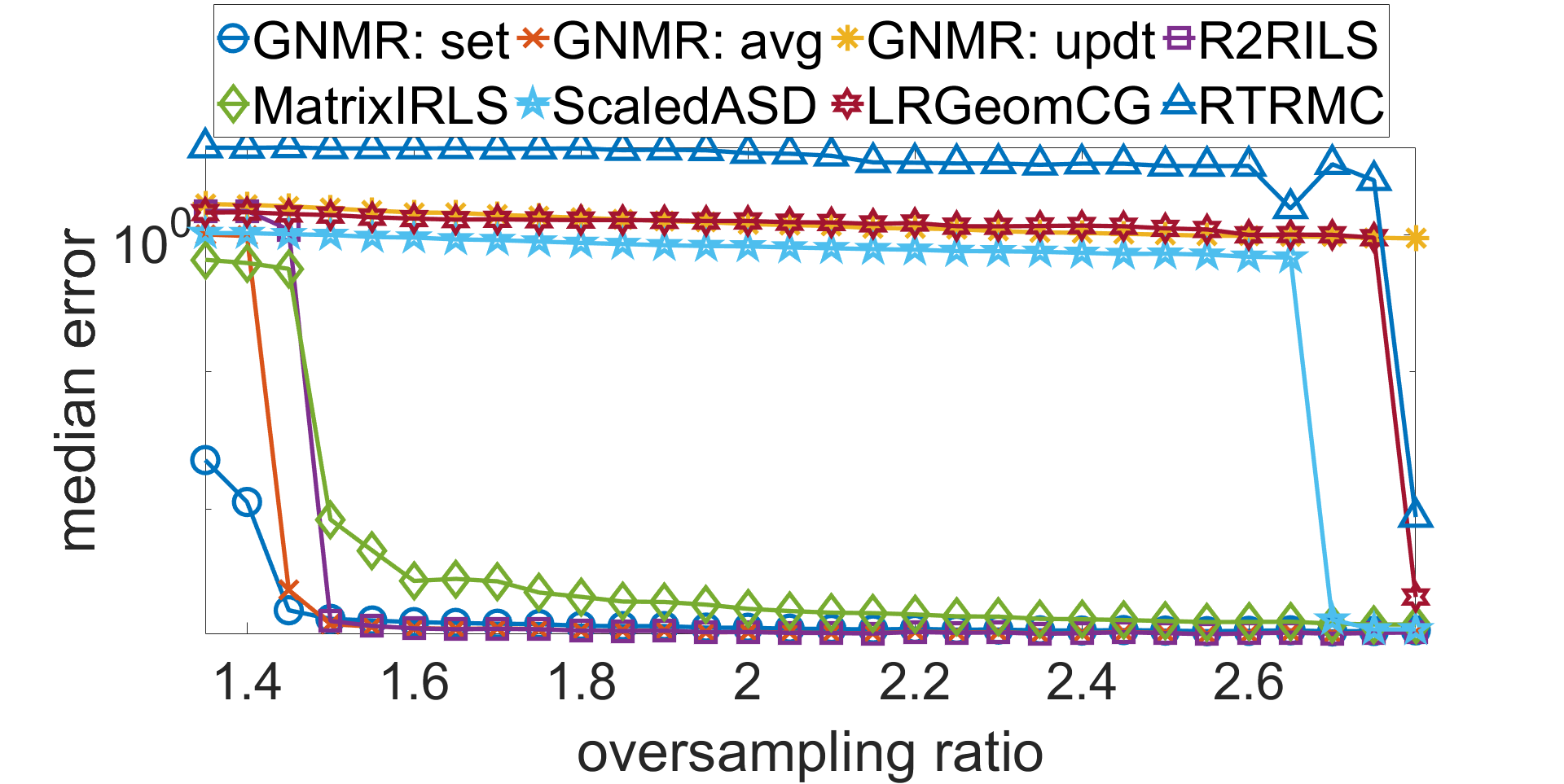
(a)

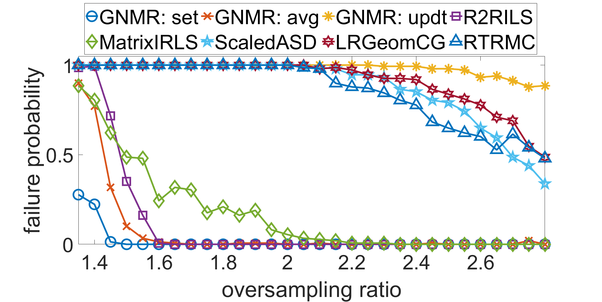
(b)

Figure 1: Comparison of several matrix completion algorithms with $X^{*}$ of size $1000\times 1000$, rank $r=5$ and condition number $\kappa=10$. Left panel: median of rel-RMSE Eq. 36; Right panel: failure probability, defined as $\text{Pr}[\texttt{rel-RMSE}>10^{-4}]$. Each point corresponds to $150$ independent realizations.

The second experiment compares R2RILS, MatrixIRLS and GNMR, which performed best in the first experiment, in a more challenging setting, where the number of observations is close to the information limit. Here $X^{*}$ is of size $n_{1}\times n_{2}=600\times 600$, rank $r=7$, and condition number $\kappa=100$ with singular values equispaced between $1$ and $\kappa$. The oversampling ratio $\rho$ ranges between $1.1$ and $1.5$. Note that for $\rho$ close to one, even if $\Omega$ contains at least $r$ entries in each row and column, the solution to the completion problem may not be unique with a non-negligible probability. Our goal in this experiment is to explore which of the algorithms can recover the matrix with essentially unlimited number of iterations. The results are depicted in Fig. 2(a). Strengthening the conclusion from the previous experiment, the setting variant Eq. 6 of GNMR outperforms the other algorithms, and succeeds in completing the matrix already at an oversampling ratio of $\rho=1.1$.

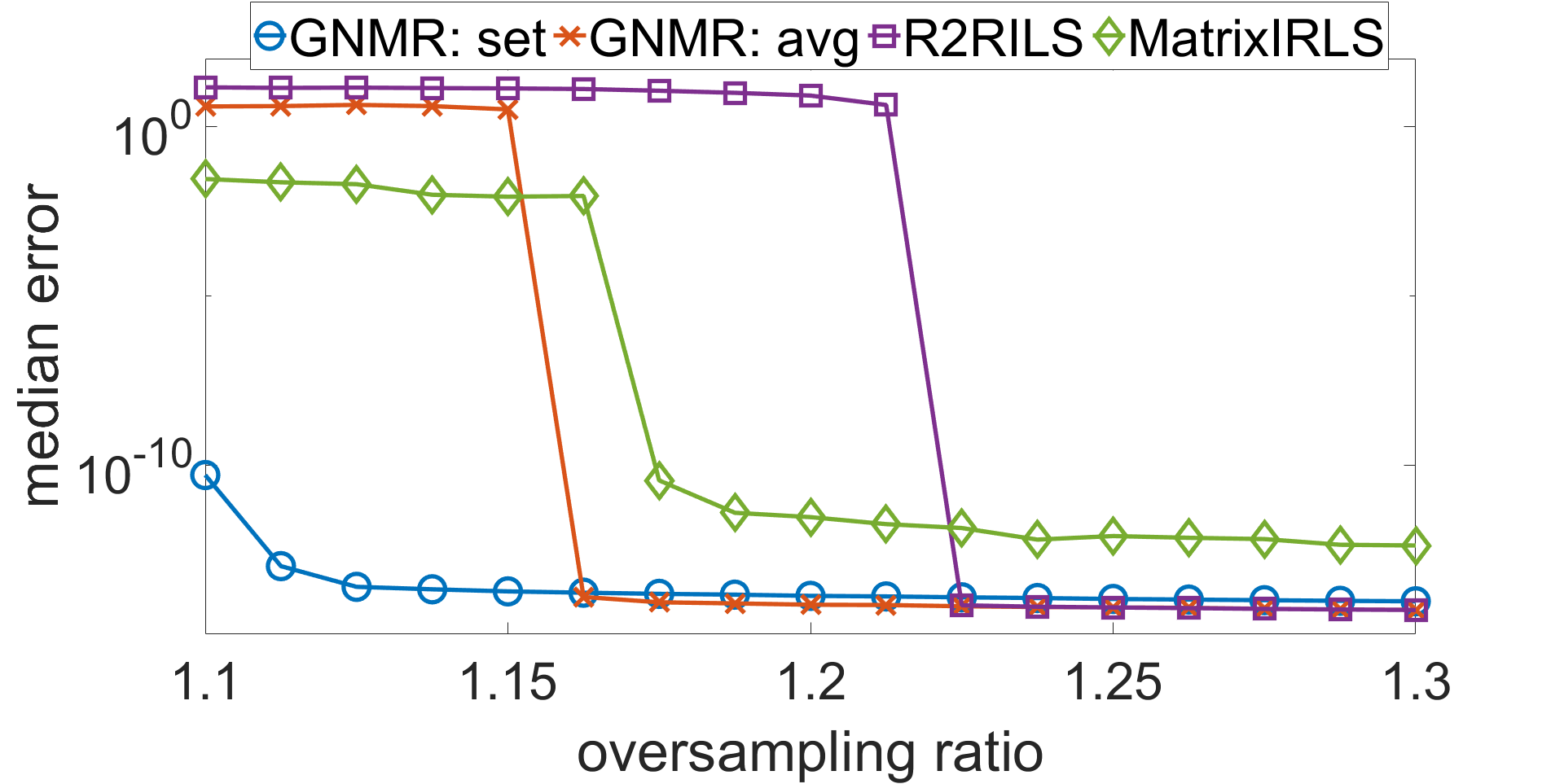
(a)

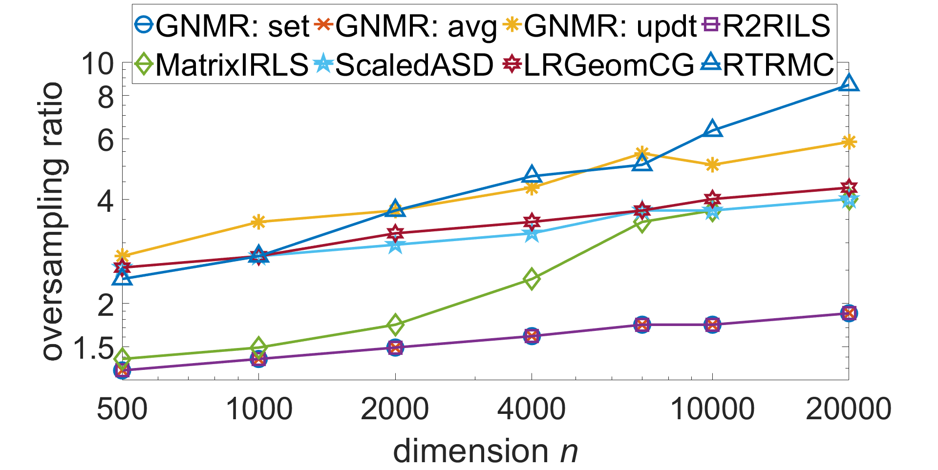
(b)

Figure 2: (a) Comparison of the algorithms which succeeded in the previous experiment. Here $X^{*}$ is of size $600\times 600$, rank $r=7$ and condition number $\kappa=100$. Each point corresponds to 150 independent realizations. (b) Comparison of several matrix completion algorithms with $X^{*}$ of varying size $n\times n$, rank $r=5$ and condition number $\kappa=10$. Y-axis is the lowest oversampling ratio from which the median of rel-RMSE is smaller than $10^{-4}$. Each point corresponds to at least 50 independent realizations.

The previous two experiments demonstrated the recovery abilities of the algorithms for matrices of relatively small dimensions. In the third experiment, our goal is to examine how increasing the dimensions affects each of the algorithms. Here $X^{*}$ is of varying size $n\times n$, fixed rank $r=5$ and condition number $\kappa=10$ with singular values equispaced between $1$ and $\kappa$. For each value of $n$, we report the lowest oversampling ratio from which the algorithm successfully recovers $X^{*}$, out of a grid of $30$ values logarithmically interpolated between $1.1$ and $4$. As seen in Fig. 2(b), only GNMR and R2RILS scale well with the dimension $n$. In fact, the results of these algorithms are ’optimal’ in the following sense. As the dimension increases, higher oversampling ratios are required to ensure that a random subset $\Omega$ satisfies the necessary condition of $r$ observed entries in each row and column of $X^{*}$ with non-negligible probability. GNMR and R2RILS successfully recovered $X^{*}$ from the lowest oversampling ratios at which this necessary condition held (see Appendix K for more details).

Next, we explore how sensitive GNMR is to the condition number of $X^{*}$. As depicted in Figs. 3 and 4(a), the setting and the averaging variants of GNMR are generally robust to the condition number in two different aspects. First, the obtained error is almost unaffected by the condition number; there is only a little sensitivity to extreme condition numbers and only at very low oversampling ratios. Second, the runtime until $\texttt{rel-RMSE}\leq 10^{-4}$ shows only little sensitivity to the condition number. The updating variant of GNMR, on the other hand, is sensitive to the condition number even at small values and at relatively large oversampling ratios.

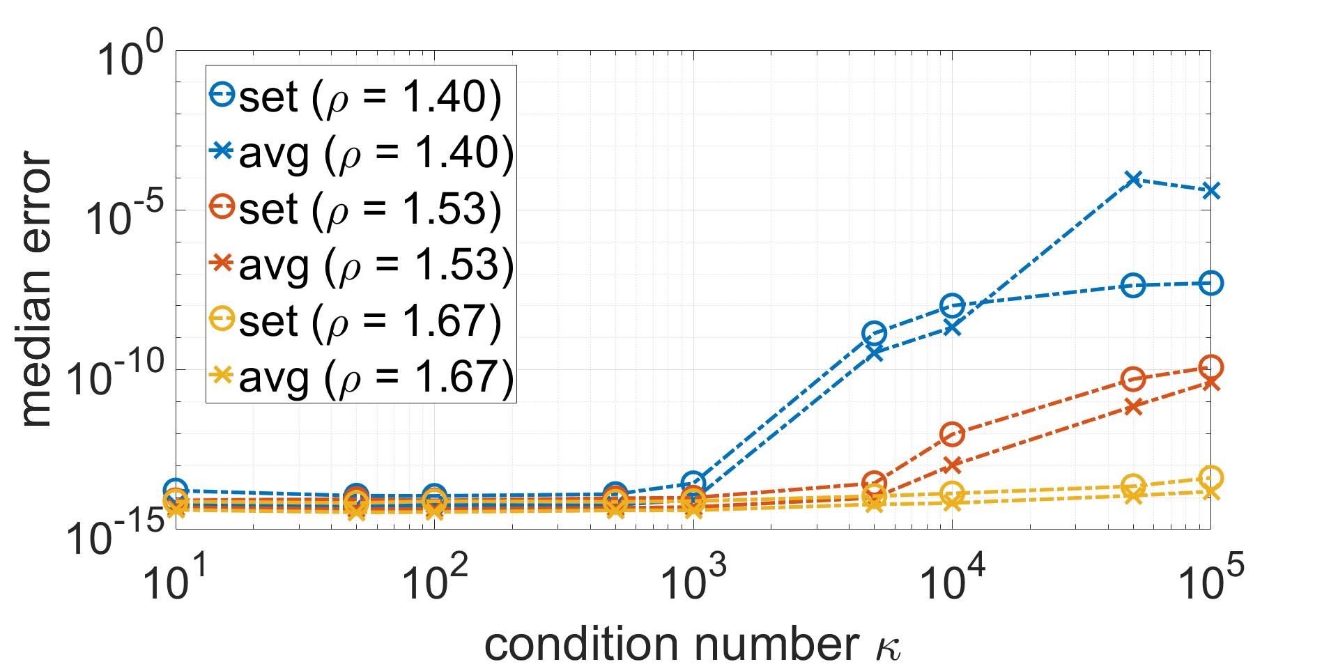
(a)

(b)

Figure 3: Median rel-RMSE of GNMR for a $1000\times 1000$ matrix $X^{*}$ of rank 5 as function of its condition number, for few values of the oversampling ratio $\rho$. Each point corresponds to 50 independent realizations.

Finally, Fig. 4(b) illustrates the stability to noise of GNMR. In this experiment, the observed entries are corrupted by additive white Gaussian noise of standard deviation $\sigma$. As seen in the figure, both the setting Eq. 6 and the averaging Eq. 7 variants of GNMR are robust to low noise levels, but interestingly, now it is the latter which performs better at higher noise levels.

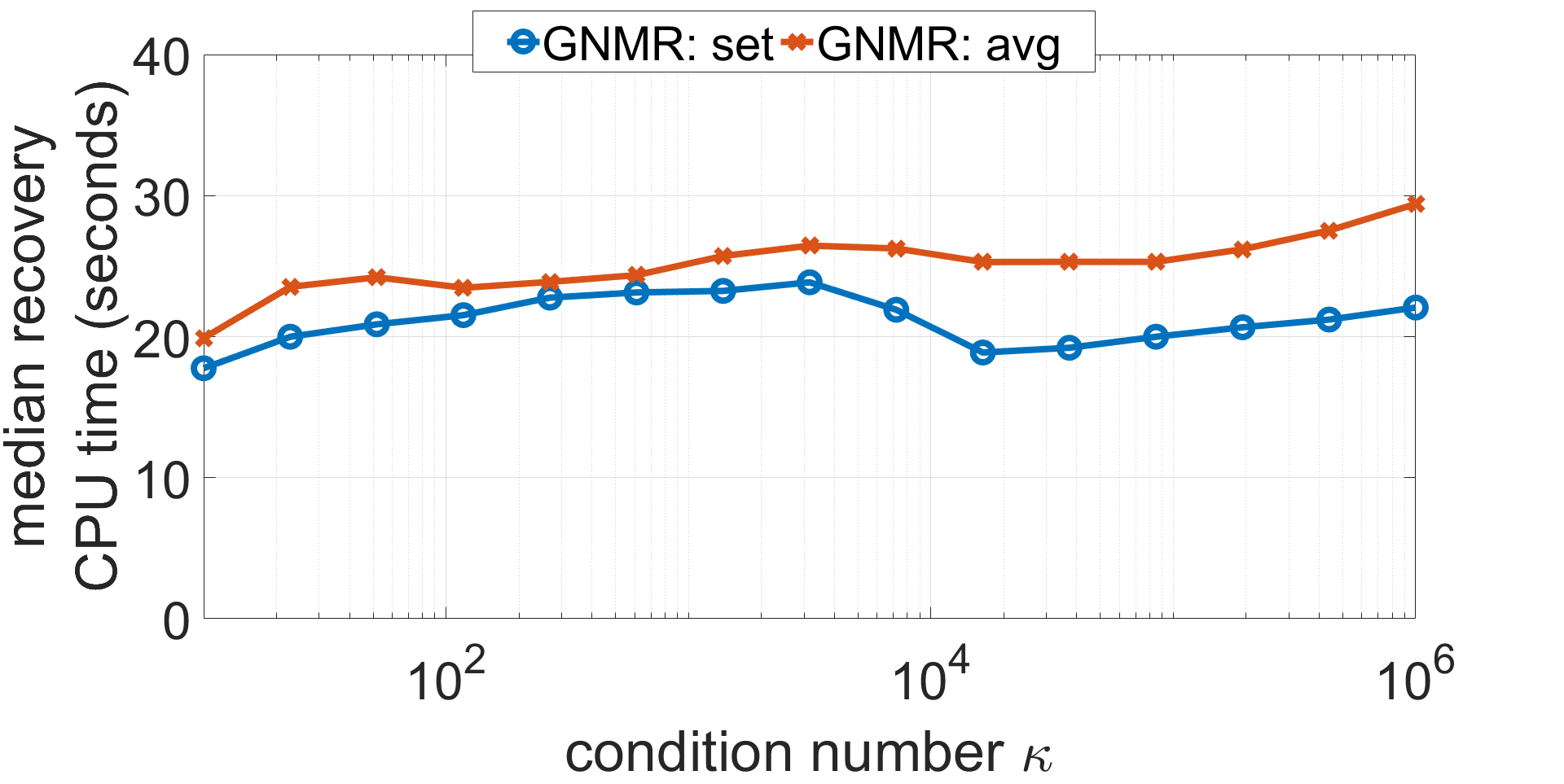
(a)

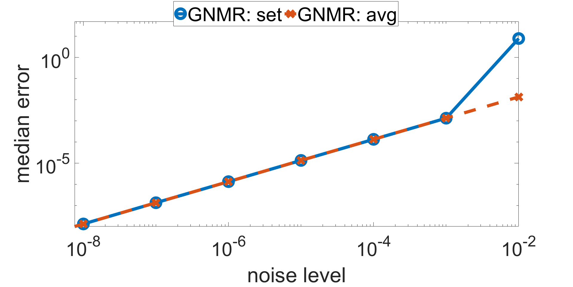
(b)

Figure 4: (a) Runtime of GNMR as function of the condition number (with $\rho=3$). (b) Stability of GNMR to additive white Gaussian noise (with $\rho=1.5$). The noise level on the x-axis corresponds to the standard deviation of the noise, and the y-axis to the median rel-RMSE. In both panels $X^{*}$ is a $1000\times 1000$ matrix of rank $5$, and each point corresponds to 150 independent realizations.

6 Discussion and future work

We proposed an extremely simple Gauss-Newton algorithm, GNMR, to solve the matrix recovery problem Eq. 1. We derived theoretical guarantees for our method, and demonstrated its state of the art empirical performance in matrix completion. In our analysis, we showed that due to the choice of the minimal norm solution to a degenerate least squares problem, the iterates of GNMR enjoy an implicit balance regularization. Similarly, we proved that the stationary points of GNMR are perfectly balanced.

The simplicity of GNMR opens several future research directions. One is related to a current gap in the literature between available guarantees for factorization-based methods and their performance in practice: Nearly all available guarantees, including ours, scale at least quadratically with the condition number $\kappa$; our simulations, however, show that GNMR is able to recover matrices with very little sensitivity to $\kappa$. As far as we are aware, the only works with $\kappa$-independent (or logarithmically scaled) guarantees are [HW14, CGJ17] and [JN15]. The latter is not factorization based, but its computational complexity is similar to factorization-based methods. However, these works employed sample splitting in their algorithm, which is never used in practice. This raises the question: is the quadratic dependence on $\kappa$ necessary for factorization-based methods that do not employ sample splitting? Our novel GNMR method, which is both simple and empirically insensitive to $\kappa$, may help in providing a negative answer to this question, possibly via a leave-one-out perturbation analysis as in [MWCC19].

Another research direction is exploiting the simplicity of GNMR to develop application-specific variants, which use additional prior knowledge or incorporate suitable regularizations. For example, in an ongoing work [ZN22] we developed a variant of GNMR for the inductive matrix completion problem [JD13, XJZ13], in which one has prior knowledge that the rows and columns of $X^{*}$ belong to certain subspaces of $\mathbb{R}^{n_{2}}$ and $\mathbb{R}^{n_{1}}$, namely that $X^{*}=AM^{*}B^{\top}$ for some known matrices $A\in\mathbb{R}^{n_{1}\times d_{1}}$, $B\in\mathbb{R}^{n_{2}\times d_{2}}$. Another example is an observed matrix corrupted by outliers, in which case the current form of GNMR is unsuitable. However, an appealing property of our Gauss-Newton framework is that the inner problem solved in each iteration is convex for any convex loss function. Hence, a robust variant of GNMR may be obtained by replacing the $\ell_{2}$ norm in Algorithm 1 by a robust one. Finally, it may be beneficial to improve the runtime of GNMR, so it will be able to handle large scale matrices.

Appendix A Comparison of GNMR to Wiberg’s method, PMF and R2RILS

In this section we compare GNMR to three other iterative matrix completion methods. In the 1970’s, several authors devised schemes to efficiently solve separable non-linear least squares problems, whose unknown variables are not necessarily matrices, see [RW80, GP03] and references therein. The idea is to divide the optimization variables to two subsets, such that solving the problem for one subset while keeping the other fixed is easy. The remaining problem for the other subset is then of reduced dimensionality. Wiberg [Wib76] adapted this idea to matrix completion as follows: Denote by $\tilde{U}(V)=\operatorname*{arg\,min}_{U}\|\mathcal{P}_{\Omega}(UV^{\top})-b\|^{2}$ the solution of the factorized objective Eq. 3 for $U$ given $V$. Then Eq. 3 can be written as an optimization problem over a single matrix $V$:

$$\min_{V}\left\|\mathcal{P}_{\Omega}\left[\tilde{U}(V)V^{\top}\right]-b\right\|^{2}.$$ (37)

At iteration $t$, Wiberg’s algorithm approximately solves Eq. 37 by the Gauss-Newton method, namely by linearizing Eq. 37 around the current estimate $V_{t}$. Similar to GNMR, the resulting least-squares problem is rank deficient, and the solution with minimal norm $\|V\|_{F}$ is chosen. Denoting this solution by ${V}_{t+1}$, Wiberg’s method then updates $U_{t+1}=\tilde{U}(V_{t+1})$. A regularized version of Wiberg’s method, which avoids the rank deficiency, became popular in the computer vision community [OD07, OYD11].

Wiberg’s algorithm is similar to GNMR, but differs from it in how $(U,V)$ are updated. Specifically, Wiberg’s algorithm applies the Gauss-Newton method to only one of the variables. Hence, in particular it treats the factor matrices $U,V$ in an asymmetric way. Empirically, in our simulations Wiberg’s method performs worse than GNMR. Also, to the best of our knowledge, no theoretical recovery guarantees have been derived for it.

The Gauss-Newton approximation for matrix completion was employed in yet another algorithm, named PMF [PT94]. However, the setting in [PT94] is slightly different from ours: instead of Eq. 3, their goal is to minimize a weighted objective $\sum_{(i,j)\in\Omega}\left(\sum_{k=1}^{r}U_{ik}V_{jk}-X^{*}_{ij}\right)^{2}/\sigma_{ij}^{2}$ for some known weights $\sigma_{ij}$. As a result, the iterative Gauss-Newton approximation yields a full-rank least squares problem with a unique solution, and there is no need to choose a specific solution as in GNMR. In addition, to the best of our knowledge, no theoretical recovery guarantees have been derived for this algorithm either.

Finally, we compare GNMR to the R2RILS algorithm [BNZ21]. Given an estimate $(U_{t},V_{t})$, the first step of R2RILS computes the minimal norm solution $(\tilde{U},\tilde{V})$ of Eq. 7a as in the averaging variant of GNMR. However, instead of the update Eq. 7b, it performs two column normalizations as follows:

$$\begin{pmatrix}U_{t+1}\\ V_{t+1}\end{pmatrix} =\begin{pmatrix}\text{ColNorm}\left[U_{t}+\text{ColNorm}[\tilde{U}]\right]\\ \text{ColNorm}\left[V_{t}+\text{ColNorm}[\tilde{V}]\right]\end{pmatrix},$$ (38)

where $\text{ColNorm}[A]$ normalizes the columns of $A$ to have unit norm. To understand the relation between the averaging variant of GNMR and R2RILS, it is instructive to analyze the latter near convergence. As R2RILS converges, $U_{t+1}\approx U_{t}$, which implies that $\text{ColNorm}[\tilde{U}]\approx U_{t}$. Hence, the update in Eq. 38 can approximately be written as $U_{t+1}\approx\tfrac{1}{2}(U_{t}+\text{ColNorm}[\tilde{U}])$, which bears resemblance to Eq. 7b. Empirically, the setting and the averaging variants of GNMR achieve superior performance over R2RILS, see Figs. 1, 2(a) and 5. In addition, the column normalizations make the theoretical analysis of R2RILS more difficult, and currently there are no recovery guarantees for it.

Appendix B Technical results

In this section we present some useful definitions and few technical results. We start by recalling the classical Weyl’s inequality, which states that for any two matrices $A,B$ of the same dimensions,

$$|\sigma_{i}(A)-\sigma_{i}(B)|\leq\|A-B\|_{2}\quad\forall i.$$ (39)

Properties of balanced SVD

Lemma B.1.

Let $X\in\mathbb{R}^{n_{1}\times n_{2}}$ be a matrix of rank $r$. Let $Z=\bigl{(}\begin{smallmatrix}U\\ V\end{smallmatrix}\bigr{)}=\text{b-SVD}(X)$ and $\Sigma\in\mathbb{R}^{r\times r}$ be the diagonal matrix with the singular values of $X$. Then $Z$ is also of rank $r$ and

$$\sigma_{r}^{2}(Z)=2\sigma_{r}(X).$$ (40)

In addition,

$$U^{\top}U=V^{\top}V=\Sigma.$$ (41)

Finally, if $X$ is $\mu$-incoherent (see Definition 3.2), then

$$\|U\|_{2,\infty}\leq\sqrt{\mu r\sigma_{1}(X)/n_{1}},\quad\|V\|_{2,\infty}\leq\sqrt{\mu r\sigma_{1}(X)/n_{2}}.$$ (42)

Proof.

Denote by $\bar{U}\Sigma\bar{V}^{\top}$ the SVD of $X$. Since $\bar{U}^{\top}U=\bar{V}^{\top}V=I$, then

$$U^{\top}U =\Sigma^{\frac{1}{2}}\bar{U}^{\top}\bar{U}\Sigma^{\frac{1}{2}}=\Sigma=\Sigma^{\frac{1}{2}}\bar{V}^{\top}\bar{V}\Sigma^{\frac{1}{2}}=V^{\top}V.$$

This proves Eq. 41. This also implies Eq. 40, since

$$\sigma^{2}_{r}(Z) =\sigma_{r}(Z^{\top}Z)=\sigma_{r}(U^{\top}U+V^{\top}V)=2\sigma_{r}(\Sigma)=2\sigma_{r}(X).$$

Finally, using $\|AB\|_{2,\infty}\leq\|A\|_{2,\infty}\|B\|_{2}$ and the $\mu$-incoherence assumption,

$$\|U\|_{2,\infty}=\|\bar{U}\Sigma^{\frac{1}{2}}\|_{2,\infty}\leq\sqrt{\sigma_{1}(X)}\|\bar{U}\|_{2,\infty}\leq\sqrt{\mu r\sigma_{1}(X)/n_{1}},$$

and similarly $\|V\|_{2,\infty}\leq\sqrt{\mu r\sigma_{1}(X)/n_{2}}$. This proves Eq. 42. ∎

A novel result on the Procrustes distance

In Section 4.2 we presented the Q-distance between factor matrices. Another distance measure, which was used in several previous works [ZL15, CBSW15, TBS⁺16, YPCC16, ZL16], is the Procrustes distance. In what follows we shall use it to bound the Q-distance.

Definition B.2.

The Procrustes distance between $Z_{1},Z_{2}\in\mathbb{R}^{n\times r}$ is defined as

$$d_{P}(Z_{1},Z_{2}) =\min\left\{\|Z_{1}-Z_{2}P\|_{F}\,\mid\,P\in\mathbb{R}^{r\times r}\text{ is orthogonal}\right\}.$$

This distance is closely related to the Wahba’s problem [Wah65]; the latter, however, allows different weights to the column norms of the difference $Z_{1}-Z_{2}P$ instead of the (uniform) Frobenius norm, but on the other hand constrains $P$ to be a rotation matrix with unit determinant. In contrast to the Q-distance, the Procrustes distance is symmetric in its arguments, and its minimizer always exists. Moreover, it can be explicitly written in terms of the SVD of $Z_{1}^{\top}Z_{2}$: The minimizer of $d_{P}(Z_{1},Z_{2})$ is $\bar{U}\bar{V}^{\top}$ where $\bar{U}\Sigma\bar{V}$ is the SVD of $Z_{1}^{\top}Z_{2}$. A simple yet useful inequality which involves the Procrustes distance is the following one.

Proposition B.3.

Let $Z_{i}=\bigl{(}\begin{smallmatrix}U_{i}\\ V_{i}\end{smallmatrix}\bigr{)}$ where $U_{i}\in\mathbb{R}^{n_{1}\times r}$, $V_{i}\in\mathbb{R}^{n_{2}\times r}$ and $r\leq\min\{n_{1},n_{2}\}$ for $i=1,2$. Then

$$\min\left\{\left|\sigma_{i}(U_{1})-\sigma_{i}(U_{2})\right|,\left|\sigma_{i}(V_{1})-\sigma_{i}(V_{2})\right|\right\} \leq d_{P}(Z_{1},Z_{2})\quad\forall i\in[r].$$

Proof.

Let $P\in\mathbb{R}^{r\times r}$ be the (orthogonal) minimizer of the Procrustes distance between $U_{1}$ and $U_{2}$. Then Weyl’s inequality Eq. 39 implies

$$\left|\sigma_{i}(U_{1})-\sigma_{i}(U_{2})\right| =\left|\sigma_{i}(U_{1})-\sigma_{i}(U_{2}P)\right|\leq\|U_{1}-U_{2}P\|_{2}\leq\|U_{1}-U_{2}P\|_{F}\leq d_{P}(Z_{1},Z_{2}),$$

and similarly for $|\sigma_{i}(V_{1})-\sigma_{i}(V_{2})|$. ∎

The next result bounds the Procrustes distance between a general pair of factor matrices and a b-SVD. Note that the following is a stronger version of [TBS⁺16, Lemma 5.14].

Lemma B.4 (Procrustes distance bound).

Let $X^{*}\in\mathbb{R}^{n_{1}\times n_{2}}$ be a matrix of rank $r$, and denote $Z^{*}=\text{b-SVD}(X^{*})$. Then for any $Z=\bigl{(}\begin{smallmatrix}U\\ V\end{smallmatrix}\bigr{)}\in\mathbb{R}^{(n_{1}+n_{2})\times r}$,

$$d_{P}^{2}(Z,Z^{*})\leq\frac{1}{(\sqrt{2}-1)\sigma_{r}\left(X^{*}\right)}\left(\|UV^{\top}-X^{*}\|_{F}^{2}+\frac{1}{4}\|U^{\top}U-V^{\top}V\|_{F}^{2}\right).$$

To prove Lemma B.4 we shall use the following auxiliary lemma [TBS⁺16, Lemma 5.4].

Lemma B.5.

For any $Z,Z^{*}\in\mathbb{R}^{(n_{1}+n_{2})\times r}$,

$$d^{2}_{P}(Z,Z^{*})\leq\frac{1}{2(\sqrt{2}-1)\sigma^{2}_{r}(Z^{*})}\|ZZ^{\top}-Z^{*}Z^{*\top}\|^{2}_{F}.$$ (43)

Proof of Lemma B.4.

Let $Z^{*}=\text{b-SVD}(X^{*})$. By Eq. 40 of Lemma B.1, we have $\sigma^{2}_{r}(Z^{*})=2\sigma_{r}(X^{*})$. In view of Eq. 43 of Lemma B.5, it thus suffices to show that

$$\|ZZ^{\top}-Z^{*}Z^{*\top}\|^{2}_{F}\leq 4\|X-X^{*}\|^{2}_{F}+\|U^{\top}U-V^{\top}V\|_{F}^{2}$$ (44)

where $X=UV^{\top}$. Note that Eq. 44, which we shall now prove, is a stronger version of [ZL16, Lemma 4]. Denote $\bigl{(}\begin{smallmatrix}U^{*}\\ V^{*}\end{smallmatrix}\bigr{)}=Z^{*}$. Then, by definition,

$$\|ZZ^{\top}-Z^{*}Z^{*\top}\|^{2}_{F}=\|UU^{\top}-U^{*}U^{*\top}\|^{2}_{F}+\|VV^{\top}-V^{*}V^{*\top}\|^{2}_{F}+2\|X-X^{*}\|_{F}^{2}.$$

We first simplify some of the terms above. By $\|AA^{\top}\|^{2}_{F}=\|A^{\top}A\|^{2}_{F}$ and Eq. 41 of Lemma B.1,

$$\|UU^{\top}-U^{*}U^{*\top}\|^{2}_{F} =\|UU^{\top}\|^{2}_{F}+\|U^{*}U^{*\top}\|^{2}_{F}-2\operatorname{Tr}\left(U^{*}U^{*\top}UU^{\top}\right),$$

$$=\|U^{\top}U\|^{2}_{F}+\|\Sigma^{*}\|^{2}_{F}-2\operatorname{Tr}\left(U^{*}U^{*\top}UU^{\top}\right),$$ (45a)

and similarly

$$\|VV^{\top}-V^{*}V^{*\top}\|^{2}_{F} =\|V^{\top}V\|^{2}_{F}+\|\Sigma^{*}\|^{2}_{F}-2\operatorname{Tr}\left(V^{*}V^{*\top}VV^{\top}\right).$$ (45b)

Let $\mathcal{E}=U^{\top}U-V^{\top}V$. By its symmetry, $\mathcal{E}$ satisfies $\operatorname{Tr}(\mathcal{E}^{2})=\operatorname{Tr}(\mathcal{E}^{\top}\mathcal{E})=\|\mathcal{E}\|_{F}^{2}$. Using the trace property $\operatorname{Tr}(AB)=\operatorname{Tr}(BA)$ for square matrices $A,B$, the first term on the RHS of Eq. 45a can be rewritten as

$$\|U^{\top}U\|^{2}_{F} =\operatorname{Tr}\left((V^{\top}V+\mathcal{E})(V^{\top}V+\mathcal{E})\right)=\|V^{\top}V\|^{2}_{F}+2\operatorname{Tr}\left(V^{\top}V\mathcal{E}\right)+\|\mathcal{E}\|_{F}^{2}.$$

Combining the above three equations gives that

$$\|ZZ^{\top}-Z^{*}Z^{*\top}\|^{2}_{F} =2\|V^{\top}V\|_{F}^{2}+2\operatorname{Tr}(V^{\top}V\mathcal{E})+\|\mathcal{E}\|_{F}^{2}+2\|\Sigma^{*}\|_{F}^{2}+2\|X-X^{*}\|_{F}^{2}$$

$$-2\operatorname{Tr}\left(U^{*}U^{*\top}UU^{\top}\right)-2\operatorname{Tr}\left(V^{*}V^{*\top}VV^{\top}\right).$$ (46)

Next, by the trace property $\operatorname{Tr}(AB)=\operatorname{Tr}(BA)$ for $A\in\mathbb{R}^{n\times r}$, $B\in\mathbb{R}^{r\times n}$ we have

$$\|X\|_{F}^{2} =\operatorname{Tr}\left(VU^{\top}UV^{\top}\right)=\operatorname{Tr}\left(V^{\top}VU^{\top}U\right)=\operatorname{Tr}\left(V^{\top}V(V^{\top}V+\mathcal{E})\right)$$

$$=\|V^{\top}V\|_{F}^{2}+\operatorname{Tr}\left(V^{\top}V\mathcal{E}\right),$$

Since $\|X-X^{*}\|^{2}_{F}=\|X\|_{F}^{2}+\|X^{*}\|_{F}^{2}-2\operatorname{Tr}(X^{*\top}X)=\|X\|_{F}^{2}+\|\Sigma^{*}\|_{F}^{2}-2\operatorname{Tr}(V^{*}U^{*\top}UV^{\top})$, we obtain that

$$\|V^{\top}V\|_{F}^{2}=\|X-X^{*}\|_{F}^{2}-\operatorname{Tr}\left(V^{\top}V\mathcal{E}\right)-\|\Sigma^{*}\|_{F}^{2}+2\operatorname{Tr}\left(V^{*}U^{*\top}UV^{\top}\right).$$

Inserting this into Eq. 46 gives that

$$\|ZZ^{\top}-Z^{*}Z^{*\top}\|^{2}_{F} =4\|X-X^{*}\|_{F}^{2}+\|\mathcal{E}\|_{F}^{2}$$

$$+2\operatorname{Tr}\left(2V^{*}U^{*\top}UV^{\top}-U^{*}U^{*\top}UU^{\top}-V^{*}V^{*\top}VV^{\top}\right).$$

Finally, using again the trace property $\operatorname{Tr}(AB)=\operatorname{Tr}(BA)$ for $A\in\mathbb{R}^{n\times r}$, $B\in\mathbb{R}^{r\times n}$, the lemma follows since

$$\operatorname{Tr}\left(U^{*}U^{*\top}UU^{\top}+V^{*}V^{*\top}VV^{\top}-2V^{*}U^{*\top}UV^{\top}\right)$$

$$=\operatorname{Tr}\left(U^{*\top}UU^{\top}U^{*}+V^{*\top}VV^{\top}V^{*}-2U^{*\top}UV^{\top}V^{*}\right)=\|U^{\top}U^{*}-V^{\top}V^{*}\|_{F}^{2}\geq 0.$$

∎

Proof of Lemma 4.7 (bounds on the Q-distance)

To prove Lemma 4.7 we shall use the following auxiliary lemma [MLC21, Lemma 1].

Lemma B.6.

Let $Z^{*}=\bigl{(}\begin{smallmatrix}U^{*}\\ V^{*}\end{smallmatrix}\bigr{)}=\text{b-SVD}(X^{*})$ where $X^{*}\in\mathbb{R}^{n_{1}\times n_{2}}$ is of rank $r$. Let $Z=\bigl{(}\begin{smallmatrix}U\\ V\end{smallmatrix}\bigr{)}\in\mathbb{R}^{(n_{1}+n_{2})\times r}$, and suppose that there exists an invertible matrix $P\in\mathbb{R}^{r\times r}$ with $1/2\leq\sigma_{r}(P)\leq\sigma_{1}(P)\leq 3/2$ such that

$$\max\{\|U^{*}-UP\|_{F},\|V^{*}-VP^{-\top}\|_{F}\}\leq\tfrac{1}{20}\sqrt{\sigma_{r}(X^{*})}.$$ (47)

Then the optimal alignment matrix $Q\in\mathbb{R}^{r\times r}$ that minimizes the Q-distance $d_{Q}(Z^{*},Z)$, exists and satisfies

$$\|P-Q\|_{2}\leq\|P-Q\|_{F}\leq\frac{5}{\sqrt{\sigma_{r}(X^{*})}}\max\{\|U^{*}-UP\|_{F},\|V^{*}-VP^{-\top}\|_{F}\}.$$

We remark that the original version of [MLC21, Lemma 1] required $\max\{\|U^{*}-UP\|_{F},\|V^{*}-VP^{-\top}\|_{F}\}\leq{\sqrt{\sigma_{r}(X^{*})}}/{80}$. However, by tracing its proof, it is straightforward to see that our version with a sharper constant also holds.

As discussed in the main text, bounding $d_{Q}(Z,Z^{*})$ is more challenging than bounding $d_{Q}(Z^{*},Z)$. Our strategy to prove the bound Eq. 29 of the first quantity is as follows. Lemma B.6 states that when the Procrustes distance $d_{P}(Z,Z^{*})$ is not too large, the optimal alignment matrix between $Z$ and $Z^{*}$ is nearly orthogonal. Intuitively, this implies that $d_{Q}(Z,Z^{*})$ is close to $d_{Q}(Z^{*},Z)$, and thus similarly bounded. In the second part of the following proof we formalize this argument.

Proof of Lemma 4.7.

Let $\tilde{Z}=\bigl{(}\begin{smallmatrix}\tilde{U}\\ \tilde{V}\end{smallmatrix}\bigr{)}=\text{b-SVD}(UV^{\top})$. First, we show that $d_{Q}(Z^{*},Z)=d_{Q}(Z^{*},\tilde{Z})$. Indeed, since $\tilde{U}\tilde{V}^{\top}=UV^{\top}$, there exists an invertible matrix $Q\in\mathbb{R}^{r\times r}$ such that $U=\tilde{U}Q$ and $V=\tilde{V}Q^{-\top}$. By definition of the Q-distance (Definition 4.5), this implies $d_{Q}(Z^{*},Z)=d_{Q}(Z^{*},\tilde{Z})$.

Next, we bound the Q-distance $d_{Q}^{2}(Z^{*},\tilde{Z})$ via the Procrustes distance. Note that for any fixed $Z_{1},Z_{2}$, it holds that $d_{Q}(Z_{1},Z_{2})\leq d_{P}(Z_{1},Z_{2})$ since the former involves minimization over any invertible matrix $Q$, whereas the latter involves minimization over a smaller subset of orthogonal matrices $P$. In particular, $d_{Q}(Z^{*},\tilde{Z})\leq d_{P}(Z^{*},\tilde{Z})=d_{P}(\tilde{Z},Z^{*})$. Invoking Lemma B.4 thus yields

$$d_{Q}^{2}(Z^{*},Z)=d_{Q}^{2}(Z^{*},\tilde{Z})\leq\frac{1}{(\sqrt{2}-1)\sigma_{r}^{*}}\left(\|UV^{\top}-X^{*}\|_{F}^{2}+\frac{1}{4}\|\tilde{U}^{\top}\tilde{U}-\tilde{V}^{\top}\tilde{V}\|_{F}^{2}\right).$$

Equation Eq. 27 of the lemma follows since the second term on the RHS vanishes due to Eq. 41 of Lemma B.1.

Next, assume Eq. 28 holds. Combining Eq. 28 and Lemma B.4 yields that there exists an orthogonal $P\in\mathbb{R}^{r\times r}$ such that

$$\|U^{*}-UP\|_{F}^{2}+\|V^{*}-VP^{-\top}\|_{F}^{2}=\|U^{*}-UP\|_{F}^{2}+\|V^{*}-VP\|_{F}^{2}\leq\frac{\sigma_{r}^{*}}{400}.$$ (48)

Hence $P$, whose all singular values are $1$, satisfies Eq. 47. Invoking Lemma B.6 implies that the optimal alignment matrix $\tilde{Q}$ between $Z^{*}$ and $Z$ exists and satisfies $\|\tilde{Q}-P\|_{2}\leq 1/4$. By the unitarity of $P$ this implies

$$\|\tilde{Q}\|_{2}\leq\|\tilde{Q}-P\|_{2}+\|P\|_{2}\leq\frac{5}{4}.$$ (49)

Next, we bound $\|\tilde{Q}^{-1}\|_{2}$. By Weyl’s inequality Eq. 39, $|\sigma_{r}(\tilde{Q})-\sigma_{r}(P)|\leq\|\tilde{Q}-P\|_{2}\leq 1/4$. Since $\sigma_{r}(P)=1$,

$$\|\tilde{Q}^{-1}\|_{2}=\frac{1}{\sigma_{r}(\tilde{Q})}\leq\frac{1}{1-1/4}=\frac{4}{3}.$$ (50)

Finally, let $\mathcal{E}_{U}=U^{*}-U\tilde{Q}$, $\mathcal{E}_{V}=V^{*}-V\tilde{Q}^{-\top}$ and $X=UV^{\top}$. Then, by the first part of the lemma Eq. 27,

$$\max\{\|\mathcal{E}_{U}\|^{2}_{F},\,\|\mathcal{E}_{V}\|^{2}_{F}\}\leq\frac{\|X-X^{*}\|_{F}^{2}}{(\sqrt{2}-1)\sigma_{r}^{*}}.$$ (51)

Let $Q=\tilde{Q}^{-1}$. Then $\|Q\|_{2}\leq 4/3$ by Eq. 50. In addition, putting everything together yields

$$\|U-U^{*}Q\|_{F}^{2}+\|V-V^{*}Q^{-\top}\|_{F}^{2} =\|\mathcal{E}_{U}Q^{-1}\|_{F}^{2}+\|\mathcal{E}_{V}Q^{\top}\|_{F}^{2}$$

$$\stackrel{{\scriptstyle(a)}}{{\leq}}\|Q^{-1}\|^{2}_{2}\|\mathcal{E}_{U}\|_{F}^{2}+\|Q\|^{2}_{2}\|\mathcal{E}_{V}\|_{F}^{2}$$

$$\stackrel{{\scriptstyle(b)}}{{\leq}}\frac{\|X-X^{*}\|_{F}^{2}}{(\sqrt{2}-1)\sigma_{r}^{*}}\left(\frac{4}{3}+\frac{5}{4}\right)$$

$$\leq\frac{25}{4}\frac{\|X-X^{*}\|_{F}^{2}}{\sigma_{r}^{*}},$$

where (a) follows from the first part of Proposition 4.8 and (b) from Eq. 49, Eq. 50 and Eq. 51. ∎

Bounds for pairs of factor matrices

Given a pair of factor matrices $\bigl{(}\begin{smallmatrix}U\\ V\end{smallmatrix}\bigr{)}$, the following lemma bounds the balance of a new pair $\bigl{(}\begin{smallmatrix}U^{\prime}\\ V^{\prime}\end{smallmatrix}\bigr{)}$ and the distance of its corresponding matrix $U^{\prime}V^{\prime\top}$ from $UV^{\top}$, in terms of the Procrustes distance.

Lemma B.7.

Let $Z=\bigl{(}\begin{smallmatrix}U\\ V\end{smallmatrix}\bigr{)},Z^{\prime}=\bigl{(}\begin{smallmatrix}U^{\prime}\\ V^{\prime}\end{smallmatrix}\bigr{)}\in\mathbb{R}^{(n_{1}+n_{1})\times r}$. Denote $d=d_{P}(Z,Z^{\prime})$ and

$$a=\sqrt{2}\max\{\sigma_{1}(U),\sigma_{1}(V)\}d+\tfrac{1}{2}d^{2}.$$

Then

$$\|U^{\prime\top}U^{\prime}-V^{\prime\top}V^{\prime}\|_{F} \leq\|U^{\top}U-V^{\top}V\|_{F}+2a,$$ (52a)

$$\|U^{\prime}V^{\prime\top}-UV^{\top}\|_{F} \leq a.$$ (52b)

Proof.

Let $P\in\mathbb{R}^{r\times r}$ be the minimizer of the Procrustes distance between $Z$ and $Z^{\prime}$, and denote $\Delta U=U^{\prime}P-U$ and $\Delta V=V^{\prime}P-V$. Then $\|\Delta U\|_{F}^{2}+\|\Delta V\|_{F}^{2}=d^{2}$. In addition, since $P$ is unitary, $U^{\prime}V^{\prime\top}=(U^{\prime}P)(V^{\prime}P)^{\top}=(U+\Delta U)(V+\Delta V)^{\top}$. Equation Eq. 52b holds since

$$\|U^{\prime}V^{\prime\top}-UV^{\top}\|_{F} \leq\|U\Delta V^{\top}\|_{F}+\|\Delta UV^{\top}\|_{F}+\|\Delta U\Delta V^{\top}\|_{F}$$

$$\stackrel{{\scriptstyle(a)}}{{\leq}}\sigma_{1}(U)\|\Delta V\|_{F}+\sigma_{1}(V)\|\Delta U\|_{F}+\|\Delta U\|_{F}\|\Delta V\|_{F}$$

$$\stackrel{{\scriptstyle(b)}}{{\leq}}\max\{\sigma_{1}(U),\sigma_{1}(V)\}\left(\|\Delta V\|_{F}+\|\Delta U\|_{F}\right)+\tfrac{1}{2}d^{2}$$

$$\stackrel{{\scriptstyle(c)}}{{\leq}}\sqrt{2}\max\{\sigma_{1}(U),\sigma_{1}(V)\}d+\tfrac{1}{2}d^{2},$$

where (a) follows from the first part of Proposition 4.8 and the Cauchy-Schwarz inequality, (b) from the inequality $ab\leq(a^{2}+b^{2})/2$, and (c) from the inequality $a+b\leq\sqrt{2(a^{2}+b^{2})}$. Next, by the triangle inequality,

$$\|U^{\prime\top}U^{\prime}-V^{\prime\top}V^{\prime}\|_{F} =\|P^{\top}\left(U^{\prime\top}U^{\prime}-V^{\prime\top}V^{\prime}\right)P\|_{F}$$

$$=\|(U+\Delta U)^{\top}(U+\Delta U)-(V+\Delta V)^{\top}(V+\Delta V)\|_{F}$$

$$\leq\|U^{\top}U-V^{\top}V\|_{F}+2\|U^{\top}\Delta U-\Delta V^{\top}V\|_{F}+\|\Delta U^{\top}\Delta U-\Delta V^{\top}\Delta V\|_{F}.$$ (53)

The last term of the RHS above can be bounded by the Cauchy-Schwarz inequality as

$$\|\Delta U^{\top}\Delta U\|_{F}+\|\Delta V^{\top}\Delta V\|_{F}\leq\|\Delta U\|_{F}^{2}+\|\Delta V\|_{F}^{2}=d^{2}.$$

As for the second term, by combining Proposition 4.8 and the inequality $a+b\leq\sqrt{2(a^{2}+b^{2})}$,

$$\|U^{\top}\Delta U-\Delta V^{\top}V\|_{F} \leq\sigma_{1}(U)\|\Delta U\|_{F}+\sigma_{1}(V)\|\Delta V\|_{F}$$

$$\leq\max\{\sigma_{1}(U),\sigma_{1}(V)\}\left(\|\Delta U\|_{F}+\|\Delta V\|_{F}\right)$$

$$\leq\sqrt{2}\max\{\sigma_{1}(U),\sigma_{1}(V)\}d.$$

Inserting these bounds into Appendix B yields Eq. 52a. ∎

Appendix C Proof of Theorem 3.3 (matrix sensing)

The proof is based on the following lemma which considers a single iteration of Algorithm 1.

Lemma C.1.

Let $\delta$ be a positive constant strictly smaller than one. Let $c_{e}=c_{e}(\delta)$ be sufficiently large. Assume the sensing operator $\mathcal{A}$ satisfies a $2r$-RIP with a constant $\delta_{2r}\leq\delta$. Let $X^{*}\in\mathbb{R}^{n_{1}\times n_{2}}$ be a matrix of rank $r$, and denote $\gamma={c_{e}}/{(2\sigma_{r}^{*})}$. Let $Z_{t}=\bigl{(}\begin{smallmatrix}U_{t}\\ V_{t}\end{smallmatrix}\bigr{)}$ be the current iterate, and denote the estimation error $e_{t}=\|X_{t}-X^{*}\|_{F}$. Also denote the minimal singular value of the factor matrices $s_{t}=\min\{\sigma_{r}(U_{t}),\sigma_{r}(V_{t})\}$ and the imbalance $l_{t}=\|U_{t}^{\top}U_{t}-V_{t}^{\top}V_{t}\|_{F}$. Assume that the current iterate satisfies the following three conditions:

$$e_{t} \leq\frac{\sigma_{r}^{*}}{c_{e}},$$ (54a)

$$s_{t} \geq\frac{1}{2}\sqrt{\sigma_{r}^{*}}+\sqrt{\frac{1+\delta}{1-\delta}}\frac{4e_{t}}{\sqrt{\sigma_{r}^{*}}},$$ (54b)

$$l_{t} \leq\frac{1}{c_{e}}\sigma_{r}^{*}-\frac{1+\delta}{1-\delta}\frac{8e_{t}^{2}}{\sigma_{r}^{*}}.$$ (54c)

Then the next iterate of Algorithm 1 with $\alpha=-1$ satisfies

$$e_{t+1} \leq\gamma e^{2}_{t},$$ (55a)

$$s_{t+1} \geq\frac{1}{2}\sqrt{\sigma_{r}^{*}}+\sqrt{\frac{1+\delta}{1-\delta}}\frac{4e_{t+1}}{\sqrt{\sigma_{r}^{*}}},$$ (55b)

$$l_{t+1} \leq\frac{1}{c_{e}}\sigma_{r}^{*}-\frac{1+\delta}{1-\delta}\frac{8e_{t+1}^{2}}{\sigma_{r}^{*}}.$$ (55c)

Proof of Theorem 3.3.

Let $Z_{0}$ be an initial guess which satisfies the conditions of the theorem. Let us show that it satisfies assumptions Eq. 54 of Lemma C.1 at $t=0$. First of all, Eq. 54a holds by the assumption $Z_{0}\in\mathcal{B}_{\text{err}}(1/c_{e})$. Next, since $Z_{0}\in\mathcal{B}_{\text{err}}(1/c_{e})\cap\mathcal{B}_{\text{bln}}(1/(2c_{e}))$, Lemma B.4 implies

$$d^{2}_{P}\left(Z_{0},Z^{*}\right)\leq\frac{1}{(\sqrt{2}-1)\sigma_{r}^{*}}\left(e^{2}_{0}+\frac{1}{4}\frac{\sigma_{r}^{*2}}{4c_{e}^{2}}\right)\leq\frac{3\sigma_{r}^{*}}{c_{e}^{2}}.$$

Hence $d^{2}_{P}(U_{0},U^{*})\leq{3\sigma_{r}^{*}}/{c_{e}^{2}}$. Combining this with Proposition B.3 yields

$$\sigma_{r}(U_{0}) \geq\sigma_{r}(U^{*})-d_{P}(Z_{0},Z^{*})\geq\sqrt{\sigma_{r}^{*}}-\frac{\sqrt{3\sigma_{r}^{*}}}{c_{e}}.$$

Together with a similar bound for $\sigma_{r}(V_{0})$ we obtain

$$s_{0}\geq\left(1-\frac{\sqrt{3}}{c_{e}}\right)\sqrt{\sigma_{r}^{*}}.$$

In addition, $e_{0}\leq\frac{\sigma_{r}^{*}}{c_{e}}$ by the assumption $Z_{0}\in\mathcal{B}_{\text{err}}(1/c_{e})$. Hence, for Eq. 54b to hold at $t=0$, we need $1-\frac{\sqrt{3}}{c_{e}}\geq\frac{1}{2}+\frac{4}{c_{e}}\sqrt{\frac{1+\delta}{1-\delta}}$. For any fixed $\delta<1$, this holds for large enough $c_{e}\equiv c_{e}(\delta)$.

Finally, we prove Eq. 54c at $t=0$. By the assumption $Z_{0}\in\mathcal{B}_{\text{bln}}(1/(2c_{e}))$, the LHS of Eq. 54c, $l_{0}$, is upper bounded by $\sigma_{r}^{*}/(2c_{e})$. In addition, by $Z_{0}\in\mathcal{B}_{\text{err}}(1/c_{e})$, the RHS of Eq. 54c is lower bounded by

$$\frac{1}{c_{e}}\sigma_{r}^{*}-\frac{1+\delta}{1-\delta}\frac{8e_{0}^{2}}{\sigma_{r}^{*}}\geq\left(1-\frac{1+\delta}{1-\delta}\frac{8}{c_{e}}\right)\frac{\sigma_{r}^{*}}{c_{e}}\geq\frac{1}{2}\frac{\sigma_{r}^{*}}{c_{e}}$$

where the last inequality follows for large enough $c_{e}\equiv c_{e}(\delta)$. Hence Eq. 54c holds at $t=0$. The theorem thus follows by iteratively applying Lemma C.1. ∎

Proof of Lemma C.1.

Let us begin with Eq. 55a. Combining assumptions Eq. 54a and Eq. 54c yields

$$e_{t}^{2}+\frac{1}{4}\|U_{t}^{\top}U_{t}-V_{t}^{\top}V_{t}\|_{F}^{2} \leq\frac{5\sigma_{r}^{*2}}{4c_{e}^{2}}.$$

Hence, for large enough $c_{e}$, the current iterate $Z_{t}$ satisfies condition Eq. 20 of Lemma 4.1. By Lemma 4.1,

$$e_{t+1}\leq\frac{1}{2}\sqrt{\frac{1+\delta}{1-\delta}}\left(\frac{25}{4\sigma_{r}^{*}}e_{t}^{2}+\Delta_{t}^{2}\right),$$

where $\Delta^{2}_{t}=\|U_{t+1}-U_{t}\|^{2}_{F}+\|V_{t+1}-V_{t}\|^{2}_{F}$. By assumption Eq. 54b, $U_{t}$ and $V_{t}$ have full column rank. Hence, $\Delta^{2}_{t}$ can be bounded by combining Lemma 4.2 and Eq. 54b as

$$\Delta_{t}^{2}\leq\frac{1+\delta}{1-\delta}\frac{e_{t}^{2}}{s_{t}^{2}}\leq\frac{1+\delta}{1-\delta}\frac{4e_{t}^{2}}{\sigma_{r}^{*}}.$$ (56)

We thus conclude

$$e_{t+1} \leq\frac{1}{2}\sqrt{\frac{1+\delta}{1-\delta}}\left[\frac{25}{4}+4\frac{1+\delta}{1-\delta}\right]\frac{e_{t}^{2}}{\sigma_{r}^{*}}.$$

Hence Eq. 55a holds for a large enough $c_{e}$.

Next, we prove Eq. 55b. By Eq. 56 we have $\|U_{t+1}-U_{t}\|_{2}\leq\Delta_{t}\leq\sqrt{\frac{1+\delta}{1-\delta}}\frac{2e_{t}}{\sqrt{\sigma_{r}^{*}}}$. Combined with Weyl’s inequality Eq. 39 and assumption Eq. 54b, this implies

$$\sigma_{r}(U_{t+1}) \geq\sigma_{r}(U_{t})-\sqrt{\frac{1+\delta}{1-\delta}}\frac{2e_{t}}{\sqrt{\sigma_{r}^{*}}}\geq\frac{1}{2}\sqrt{\sigma_{r}^{*}}+\sqrt{\frac{1+\delta}{1-\delta}}\frac{2e_{t}}{\sqrt{\sigma_{r}^{*}}}.$$

Together with a similar bound on $\sigma_{r}(V_{t+1})$ we obtain

$$s_{t+1}\geq\frac{1}{2}\sqrt{\sigma_{r}^{*}}+\sqrt{\frac{1+\delta}{1-\delta}}\frac{2e_{t}}{\sqrt{\sigma_{r}^{*}}}.$$ (57)

In addition, combining Eq. 55a and Eq. 54a yields

$$e_{t+1}\leq\tfrac{1}{2}e_{t}.$$ (58)

Inequality Eq. 55b follows by inserting Eq. 58 into Eq. 57.

Finally, we prove Eq. 55c. By assumption Eq. 54b, $U_{t}$ and $V_{t}$ have full column rank. Invoking Lemma 4.3 thus gives that

$$l_{t+1}=\|U_{t+1}^{\top}U_{t+1}-V_{t+1}^{\top}V_{t+1}\|_{F} \leq\|U_{t}^{\top}U_{t}-V_{t}^{\top}V_{t}\|_{F}+\frac{1+\delta}{1-\delta}\frac{e_{t}^{2}}{s_{t}^{2}}.$$

Bounding the first term on the RHS by assumption Eq. 54c and the second term by Eq. 56 yields

$$l_{t+1} \leq\frac{\sigma_{r}^{*}}{c_{e}}-\frac{1+\delta}{1-\delta}\frac{8e_{t}^{2}}{\sigma_{r}^{*}}+\frac{1+\delta}{1-\delta}\frac{4e_{t}^{2}}{\sigma_{r}^{*}}=\frac{\sigma_{r}^{*}}{c_{e}}-\frac{1+\delta}{1-\delta}\frac{4e_{t}^{2}}{\sigma_{r}^{*}}.$$

Inequality Eq. 55c follows by combining this with Eq. 58. ∎

Appendix D Proof of Theorem 3.4 (noisy matrix sensing)

The proof is based on the following lemma which considers a single iteration of Algorithm 2.

Lemma D.1.

Let $\delta$ be a positive constant strictly smaller than one, and denote $c=7(1+\delta)^{\frac{3}{2}}/(1-\delta)^{\frac{3}{2}}$. Assume the sensing operator $\mathcal{A}$ satisfies a $2r$-RIP with a constant $\delta_{2r}\leq\delta$. Let $b=\mathcal{A}(X^{*})+\xi$ where $X^{*}\in\mathbb{R}^{n_{1}\times n_{2}}$ is of rank $r$ and $\xi\in\mathbb{R}^{m}$ satisfies

$$\|\xi\|\leq\frac{\sigma_{r}^{*}\sqrt{1-\delta}}{6c}.$$ (59)

Denote $\gamma=c/(4\sigma_{r}^{*})$. Let $Z_{t}=\bigl{(}\begin{smallmatrix}U_{t}\\ V_{t}\end{smallmatrix}\bigr{)}$ be the current iterate. Assume that its estimation error $e_{t}=\|X_{t}-X^{*}\|_{F}$ satisfies

$$e_{t} \leq\frac{\sigma_{r}^{*}}{c}+\frac{3\|\xi\|}{\sqrt{1-\delta}}.$$ (60)

Then the next iterate of Algorithm 2 with $\alpha=-1$ satisfies

$$e_{t+1} \leq\gamma e^{2}_{t}+\frac{3\|\xi\|}{\sqrt{1-\delta}}.$$ (61)

Proof of Theorem 3.4.

By assumption, at $t=0$ the error satisfies

$$\|X_{0}-X^{*}\|_{F}\leq\frac{\sigma_{r}^{*}}{c}.$$ (62)

Hence Eq. 60 holds at $t=0$. The proof follows by induction: We show that if Eq. 60 holds at iteration $t$, then it holds at $t$. By combining Eqs. 59 and 60,

$$\gamma e^{2}_{t} \leq\frac{c}{4\sigma_{r}^{*}}\left(\frac{\sigma_{r}^{*}}{c}+\frac{3\|\xi\|}{\sqrt{1-\delta}}\right)^{2}\leq\left(1+\frac{3}{6}\right)^{2}\frac{\sigma_{r}^{*}}{4c}\leq\frac{\sigma_{r}^{*}}{c}.$$

Plugging this into Eq. 61 of Lemma D.1 yields $e_{t+1}\leq\frac{\sigma_{r}^{*}}{c}+\frac{3\|\xi\|}{\sqrt{1-\delta}}$, namely Eq. 60 holds at iteration $t+1$. Equation Eq. 14 of the theorem follows by iteratively applying Lemma D.1.

Next, let $x=3\|\xi\|/\sqrt{1-\delta}$. We shall prove by induction that

$$\|X_{t}-X^{*}\|_{F}\leq\frac{1}{4^{2^{t}-1}}\frac{\sigma_{r}^{*}}{c}+2x.$$ (63)

At $t=0$, Eq. 63 follows by the initialization assumption Eq. 62. By combining Eqs. 62 and D.1, Eq. 63 holds also at $t=1$, since

$$\|X_{1}-X^{*}\|_{F}\leq\gamma\|X_{0}-X^{*}\|_{F}^{2}+x\leq\frac{\sigma_{r}^{*}}{4c}+x\leq\frac{\sigma_{r}^{*}}{4c}+2x.$$

Next, assume Eq. 63 holds at some $t\geq 1$. Then

$$\|X_{t+1}-X^{*}\|_{F} \leq\gamma\|X_{t}-X^{*}\|_{F}^{2}+x\leq\frac{c}{4\sigma_{r}^{*}}\left(\frac{1}{4^{2^{t}-1}}\frac{\sigma_{r}^{*}}{c}+2x\right)^{2}+x$$

$$=\frac{1}{4^{2^{{t}+1}-1}}\frac{\sigma_{r}^{*}}{c}+\frac{1}{4^{2^{t}-1}}x+\frac{c}{\sigma_{r}^{*}}x^{2}+x\leq\frac{1}{4^{2^{{t}+1}-1}}\frac{\sigma_{r}^{*}}{c}+\left(\frac{1}{4^{2^{t}-1}}+\frac{3}{2}\right)x,$$

where the last inequality follows by the assumption $x\leq\sigma_{r}^{*}/(2c)$ Eq. 59. Since $\frac{1}{4^{2^{t}-1}}+\frac{3}{2}\leq 2$ for any $t\geq 1$, Eq. 63 holds at $t+1$. This completes the proof. ∎

Proof of Lemma D.1.

The proof consists of two parts. First, we show that the next error is bounded as

$$e_{t+1} \leq\frac{1}{2(\sqrt{2}-1)}\sqrt{\frac{1+\delta}{1-\delta}}\frac{e_{t}^{2}}{\sigma_{r}^{*}}+\frac{1}{2}\sqrt{\frac{1+\delta}{1-\delta}}\|\Delta Z_{t}\|_{F}^{2}+\frac{2}{\sqrt{1-\delta}}\|\xi\|$$ (64)

where $\Delta Z_{t}$ is the minimal norm solution to the least squares problem of Eq. 4a. Second, we show that

$$\|\Delta Z_{t}\|_{F}^{2}\leq\frac{1+\delta}{1-\delta}\frac{e_{t}^{2}}{\sigma_{r}^{*}}+\frac{1}{2\sqrt{1+\delta}}\|\xi\|.$$ (65)

Combining these bounds gives

$$e_{t+1} \leq\frac{1}{2(\sqrt{2}-1)}\sqrt{\frac{1+\delta}{1-\delta}}\frac{e_{t}^{2}}{\sigma_{r}^{*}}+\frac{1}{2}\sqrt{\frac{1+\delta}{1-\delta}}\left(\frac{1+\delta}{1-\delta}\frac{e_{t}^{2}}{\sigma_{r}^{*}}+\frac{1}{2\sqrt{1+\delta}}\|\xi\|\right)+\frac{2}{\sqrt{1-\delta}}\|\xi\|$$

$$=\frac{1}{2}\sqrt{\frac{1+\delta}{1-\delta}}\left(\frac{1}{\sqrt{2}-1}+\frac{1+\delta}{1-\delta}\right)\frac{e_{t}^{2}}{\sigma_{r}^{*}}+\frac{9/4}{\sqrt{1-\delta}}\|\xi\|.$$

Plugging the definitions $c=7(1+\delta)^{\frac{3}{2}}/(1-\delta)^{\frac{3}{2}}$ and $\gamma=c/(4\sigma_{r}^{*})$ yields Eq. 61, as

$$e_{t+1} \leq\frac{c}{14}\left(\frac{1}{\sqrt{2}-1}+1\right)\frac{e_{t}^{2}}{\sigma_{r}^{*}}+\frac{9/4}{\sqrt{1-\delta}}\|\xi\|\leq\gamma e_{t}^{2}+\frac{3}{\sqrt{1-\delta}}\|\xi\|.$$

The proof of Eq. 64 follows the lines of the proof of Lemma 4.1, but uses the Procrustes distance instead of the Q-distance. Let $P$ be the minimizer of the Procrustes distance between $Z_{t}$ and $Z^{*}$, and denote $Z=\bigl{(}\begin{smallmatrix}U\\ V\end{smallmatrix}\bigr{)}=\bigl{(}\begin{smallmatrix}U^{*}P\\ V^{*}P\end{smallmatrix}\bigr{)}$ where $\bigl{(}\begin{smallmatrix}U^{*}\\ V^{*}\end{smallmatrix}\bigr{)}=\text{b-SVD}(X^{*})$. Then, by Lemma B.4, $\Delta Z=Z_{t}-Z$ satisfies

$$\|\Delta Z\|_{F}^{2}\leq\frac{1}{(\sqrt{2}-1)\sigma_{r}^{*}}\left(e_{t}^{2}+\frac{1}{4}\|U_{t}^{\top}U_{t}-V_{t}^{\top}V_{t}\|_{F}^{2}\right)=\frac{e_{t}^{2}}{(\sqrt{2}-1)\sigma_{r}^{*}},$$ (66)

where the equality follows by the fact that $U_{t},V_{t}$ are balanced due to the additional SVD step of the algorithm, see Eq. 41 of Lemma B.1. Let $F_{t}^{2}$ be the objective function of the least squares problem. Denote $\bigl{(}\begin{smallmatrix}\Delta U\\ \Delta V\end{smallmatrix}\bigr{)}=\Delta Z$. Using $UV^{\top}=X^{*}$,

$$F_{t}\left(\Delta Z\right) =\left\|\mathcal{A}\left(U_{t}V_{t}^{\top}+U_{t}\Delta V^{\top}+\Delta UV_{t}^{\top}\right)-b\right\|$$

$$=\left\|\mathcal{A}\left(U_{t}V_{t}^{\top}+U_{t}\Delta V^{\top}+\Delta UV_{t}^{\top}-UV^{\top}\right)-\xi\right\|.$$

Since $U_{t}V_{t}+U_{t}\Delta V^{\top}+\Delta UV_{t}^{\top}-UV^{\top}=-\Delta U\Delta V^{\top}$,

$$F_{t}(\Delta Z) =\|\mathcal{A}\left(\Delta U\Delta V^{\top}\right)+\xi\|\leq\|\mathcal{A}\left(\Delta U\Delta V^{\top}\right)\|+\|\xi\|\leq\sqrt{1+\delta_{r}}\|\Delta U\Delta V^{\top}\|_{F}+\|\xi\|,$$ (67)

where the last inequality follows by the fact that $\mathcal{A}$ satisfies an r-RIP with a constant $\delta_{r}$. By the Cauchy-Schwarz inequality and the fact that $ab\leq(a^{2}+b^{2})/2$, we have $\|\Delta U\Delta V^{\top}\|_{F}\leq(\|\Delta U\|_{F}^{2}+\|\Delta V\|_{F}^{2})/2=\|\Delta Z\|_{F}^{2}/2$. Combining this with Eqs. 66 and 67 yields

$$F_{t}(\Delta Z)\leq\frac{\sqrt{1+\delta_{r}}}{2(\sqrt{2}-1)\sigma_{r}^{*}}e_{t}^{2}+\|\xi\|.$$ (68)

Next, we lower bound $F_{t}$ at the minimal norm solution $\Delta Z_{t}$. Similar to the proof of Eq. 31, any feasible solution to the least squares problem, including $\Delta Z_{t}$, satisfies

$$F_{t}(\Delta Z_{t}) =\|\mathcal{A}\left(U_{t}V_{t}+U_{t}\Delta V_{t}^{\top}+\Delta U_{t}V_{t}^{\top}-X^{*}\right)-\xi\|=\|\mathcal{A}\left(X_{t+1}-\Delta U_{t}\Delta V_{t}^{\top}-X^{*}\right)-\xi\|$$

$$\geq\|\mathcal{A}(X_{t+1}-X^{*})\|-\|\mathcal{A}(\Delta U_{t}\Delta V_{t}^{\top})\|-\|\xi\|.$$

Using again the RIP of $\mathcal{A}$, the Cauchy-Schwarz inequality and $ab\leq(a^{2}+b^{2})/2$ yields

$$F_{t}(\Delta Z_{t}) \geq\sqrt{1-\delta_{2r}}e_{t+1}-\frac{\sqrt{1+\delta_{r}}}{2}\|\Delta Z_{t}\|_{F}^{2}-\|\xi\|.$$ (69)

Since $\Delta Z_{t}$ minimizes $F_{t}$ by construction, in particular $F_{t}(\Delta Z_{t})\leq F_{t}(\Delta Z)$. Hence, combining Eqs. 68 and 69 with the assumption $\delta_{2r}\leq\delta$ yields Eq. 64.

Next, we prove Eq. 65. By tracing the proof of Lemma 4.2, it is easy to verify that in the noisy case,

$$\|\Delta Z_{t}\|_{F}^{2} \leq\frac{1+\delta_{2r}}{1-\delta_{2r}}\frac{(e_{t}+\|\xi\|)^{2}}{\min\{\sigma_{r}^{2}(U_{t}),\sigma_{r}^{2}(V_{t})\}}\leq\frac{1+\delta}{1-\delta}\frac{(e_{t}+\|\xi\|)^{2}}{\min\{\sigma_{r}^{2}(U_{t}),\sigma_{r}^{2}(V_{t})\}}.$$ (70)

By combining Proposition B.3 with Eq. 66 we obtain

$$\sigma_{r}(U_{t})\geq\sigma_{r}(U^{*})-d_{P}(U_{t},U^{*})\geq\sqrt{\sigma_{r}^{*}}-\|\Delta Z\|_{F}\geq\sqrt{\sigma_{r}^{*}}-\frac{e_{t}}{\sqrt{(\sqrt{2}-1)\sigma_{r}^{*}}}.$$

Employing assumptions Eqs. 59 and 60 yields

$$\sigma_{r}(U_{t})\geq\left(1-\frac{1}{c}-\frac{3}{6c}\right)\frac{\sqrt{\sigma_{r}^{*}}}{\sqrt{\sqrt{2}-1}}\geq\frac{\sqrt{\sigma_{r}^{*}}}{\sqrt{2(\sqrt{2}-1)}},$$

where the last inequality follows since $c=7(1+\delta)^{\frac{3}{2}}/(1-\delta)^{\frac{3}{2}}\geq 7$. Together with a similar bound on $\sigma_{r}(V_{t})$ and employing again assumptions Eqs. 59 and 60, Eq. 70 gives that

$$\|\Delta Z_{t}\|_{F}^{2} \leq 2(\sqrt{2}-1)\frac{1+\delta}{1-\delta}\frac{(e_{t}+\|\xi\|)^{2}}{\sigma_{r}^{*}}=2(\sqrt{2}-1)\frac{1+\delta}{1-\delta}\left(\frac{e_{t}^{2}}{\sigma_{r}^{*}}+\frac{2e_{t}+\|\xi\|}{\sigma_{r}^{*}}\|\xi\|\right)$$

$$\leq 2(\sqrt{2}-1)\frac{1+\delta}{1-\delta}\left(\frac{e_{t}^{2}}{\sigma_{r}^{*}}+\frac{2\cdot(1+3/6)+1/6}{c}\|\xi\|\right)\leq\frac{1+\delta}{1-\delta}\frac{e_{t}^{2}}{\sigma_{r}^{*}}+\frac{1}{2\sqrt{1+\delta}}\|\xi\|.$$

This completes the proof of Eq. 65. ∎

Appendix E Proof of Theorem 3.9 (uniform RIP for matrix completion)

Before we present the proofs for the matrix completion setting, we make the following two remarks.

Remark E.1.

Our results for matrix completion (Theorems 3.5, 3.7 and 3.9) are stated with respect to a uniform random model of the sampling pattern, namely $\Omega$ is drawn uniformly from $2^{[n_{1}]\times[n_{2}]}$ with fixed size $|\Omega|$. Similar to previous works, our analysis assumes the more convenient Bernoulli model, in which each entry of $X^{*}$ is observed with probability $p$. These models are equivalent in the sense that under the Bernoulli model, $pn_{1}n_{2}-C\sqrt{n_{2}\log n_{2}}\leq|\Omega|\leq pn_{1}n_{2}+C\sqrt{n_{2}\log n_{2}}$ with probability $1-1/n^{10}$ where $C$ is a constant [KMO10, section I.D]. Consequently, a result that holds w.p. $1-\mathcal{O}(1/n^{c})$ for some $c\leq 10$ under the uniform random model with a certain $|\Omega|$, holds with similar probability under the Bernoulli model with $p\equiv\frac{|\Omega|}{n_{1}n_{2}}$.

Remark E.2.

In our results, if an argument holds for some constants (such as $C,c_{e},c_{l}$, etc.), then it also holds for larger constants. As a consequence, if, for example, Lemma A claims that there exists a constant $c_{1}$ such that argument A$(c_{1})$ holds, and Lemma B claims that there exists an a constant $c_{2}$ such that argument B$(c_{2})$ holds, then there exists a constant $c_{3}$ such that arguments A$(c_{3})\land$B$(c_{3})$ hold, as we can always choose $c_{3}\geq\max\{c_{1},c_{2}\}$.

The proof of Theorem 3.9 relies on the following two technical lemmas. The first lemma provides bounds on two distance measures between $Z\in\mathcal{B}_{\textnormal{err}}({\epsilon}/{c_{e}})\cap\mathcal{B}_{\textnormal{bln}}({1}/{c_{l}})\cap\mathcal{B}_{\mu}$ and a nearby $Z^{*}\in\mathcal{\mathcal{missing}}B^{*}\cap\mathcal{B}_{\mu}$. The second lemma states that theses bounds are sufficient for the RIP Eq. 16 to hold. These lemmas are also used in the proof of Theorems 3.5 and 3.7.

Lemma E.3.

There exist constants $C,c_{l},c_{e}$ such that the following holds. Let $X^{*}\in\mathcal{M}(n_{1},n_{2},r,\mu,\kappa)$ and $\epsilon\in(0,1)$, and assume $\Omega\subseteq[n_{1}]\times[n_{2}]$ is randomly sampled with $np\geq C\max\{\log n,{\mu^{2}r^{2}\kappa^{2}}/{\epsilon^{4}}\}$. Then w.p. at least $1-{2}/{n^{5}}$, for any $\bigl{(}\begin{smallmatrix}U\\ V\end{smallmatrix}\bigr{)}\in\mathcal{B}_{\textnormal{err}}({\epsilon}/{c_{e}})\cap\mathcal{B}_{\textnormal{bln}}({1}/{c_{l}})\cap\mathcal{B}_{\mu}$ with $X=UV^{\top}$ there exists $\bigl{(}\begin{smallmatrix}U^{*}\\ V^{*}\end{smallmatrix}\bigr{)}\in\mathcal{B}^{*}\cap\mathcal{B}_{\mu}$ such that

$$\|U-U^{*}\|^{2}_{F}+\|V-V^{*}\|^{2}_{F} \leq\frac{\epsilon}{2}\|X-X^{*}\|_{F},$$ (71a)

$$\frac{1}{\sqrt{p}}\|(U-U^{*})(V-V^{*})^{\top}\|_{F(\Omega)} \leq\frac{\epsilon}{6}\|X-X^{*}\|_{F}.$$ (71b)

In what follows, we denote by $\mathcal{M}(n_{1},n_{2},r,\mu)$ the set of $n_{1}\times n_{2}$ $\mu$-incoherent matrices of rank $r$, without specifying the condition number.

Lemma E.4.

There exists a constant $C$ such that the following holds. Let $X^{*}\in\mathcal{M}(n_{1},n_{2},r,\mu)$ and $\epsilon\in(0,1)$, and assume $\Omega\subseteq[n_{1}]\times[n_{2}]$ is randomly sampled with $np\geq\frac{C}{\epsilon^{2}}\mu r\log n$. Then w.p. at least $1-{3}/{n^{3}}$, for any $\bigl{(}\begin{smallmatrix}U\\ V\end{smallmatrix}\bigr{)}\in\mathbb{R}^{(n_{1}+n_{2})\times r}$ for which there exists $\bigl{(}\begin{smallmatrix}U^{*}\\ V^{*}\end{smallmatrix}\bigr{)}\in\mathcal{B}^{*}$ that satisfies Eq. 71, the RIP Eq. 16 holds w.r.t. $X=UV^{\top}$.

Proof of Theorem 3.9.

By Lemma E.3, there exists $\bigl{(}\begin{smallmatrix}U^{*}\\ V^{*}\end{smallmatrix}\bigr{)}\in\mathcal{B}^{*}$ such that Eq. 71 holds. The theorem thus follows by Lemma E.4. ∎

Proofs of Lemmas E.3 and E.4

Let us begin with two auxiliary lemmas. The first lemma provides a (deterministic) bound on the Frobenius distance between $Z\in\mathcal{B}_{\textnormal{err}}({1}/{c_{e}})\cap\mathcal{B}_{\textnormal{bln}}({1}/{c_{l}})$ and a nearby $Z^{*}\in\mathcal{B}^{*}\cap\mathcal{B}_{\mu}$.

Lemma E.5.

There exist constants $c_{l},c_{e}$ such that the following holds. Let $X^{*}\in\mathcal{M}(n_{1},n_{2},r,\mu)$. Then for any $\bigl{(}\begin{smallmatrix}U\\ V\end{smallmatrix}\bigr{)}\in\mathcal{B}_{\textnormal{err}}({1}/{c_{e}})\cap\mathcal{B}_{\textnormal{bln}}({1}/{c_{l}})$ there exists $\bigl{(}\begin{smallmatrix}U^{*}\\ V^{*}\end{smallmatrix}\bigr{)}\in\mathcal{B}^{*}\cap\mathcal{B}_{\mu}$ such that

$$\|U-U^{*}\|_{F}^{2}+\|V-V^{*}\|_{F}^{2} \leq\frac{25}{4\sigma_{r}^{*}}\|UV^{\top}-X^{*}\|_{F}^{2}.$$ (72)

The second lemma is a direct consequence of [KMO10, Lemma 7.1].

Lemma E.6.

There exist constants $C,c$ such that the following holds for any $\mu,t,\epsilon>0$. Assume $\Omega\subseteq[n_{1}]\times[n_{2}]$ is randomly sampled with $np\geq C\max\{\log n,\mu^{2}r^{2}/\epsilon^{4}\}$. Then w.p. at least $1-{2}/{n^{5}}$, for any $\bigl{(}\begin{smallmatrix}U\\ V\end{smallmatrix}\bigr{)}\in\mathbb{R}^{(n_{1}+n_{2})\times r}$ such that

$$\|U\|_{2,\infty}\leq 4\sqrt{\mu rt/n_{1}},\quad\|V\|_{2,\infty}\leq 4\sqrt{\mu rt/n_{2}},$$ (73)

we have

$$\frac{1}{p}\|UV^{\top}\|^{2}_{F(\Omega)}\leq\frac{\|U\|_{F}^{2}+\|V\|_{F}^{2}}{2}\left(c\left(\|U\|_{F}^{2}+\|V\|_{F}^{2}\right)+t\epsilon^{2}\right).$$ (74)

Proof of Lemma E.3.

Given $Z=\bigl{(}\begin{smallmatrix}U\\ V\end{smallmatrix}\bigr{)}$, let $Z^{*}=\bigl{(}\begin{smallmatrix}U^{*}\\ V^{*}\end{smallmatrix}\bigr{)}\in\mathcal{B}^{*}\cap\mathcal{B}_{\mu}$ be the corresponding factor matrices from Lemma E.5. We shall prove that $Z^{*}$ satisfies Eq. 71 w.p. at least $1-{1}/{n^{5}}$. First, by $Z\in\mathcal{B}_{\textnormal{err}}({\epsilon}/{c_{e}})$ we have $\|X-X^{*}\|_{F}\leq{\epsilon\sigma_{r}^{*}}/{c_{e}}$. Equation Eq. 71a follows for large enough $c_{e}$ by combining this with Eq. 72 of Lemma E.5.

Next, we prove Eq. 71b. Since both $Z,Z^{*}\in\mathcal{B}_{\mu}$, the difference $\Delta U^{*}=U-U^{*}$ satisfies

$$\|\Delta U^{*}\|_{2,\infty} \leq\|U\|_{2,\infty}+\|U^{*}\|_{2,\infty}\leq 2\sqrt{3\mu r\sigma_{1}^{*}/n_{1}},$$

and similarly $\|\Delta V^{*}\|_{2,\infty}\leq 2\sqrt{3\mu r\sigma_{1}^{*}/n_{2}}$ where $\Delta V^{*}=V-V^{*}$. Invoking Lemma E.6 with $t\to\sigma_{1}^{*}$ and $\epsilon\to\epsilon/(11\sqrt{\kappa})$ yields

$$\frac{1}{p}\|\Delta U^{*}\Delta V^{*\top}\|^{2}_{F(\Omega)} \leq\frac{\|\Delta U^{*}\|_{F}^{2}+\|\Delta V^{*}\|_{F}^{2}}{2}\left(c\left(\|\Delta U^{*}\|_{F}^{2}+\|\Delta V^{*}\|_{F}^{2}\right)+\frac{\epsilon^{2}\sigma_{r}^{*}}{121}\right).$$ (75)

Next, we bound $\|\Delta U^{*}\|_{F}^{2}+\|\Delta V^{*}\|_{F}^{2}$. To this end, recall that $Z^{*}$ are the factor matrices given by Lemma E.5. Combining Eq. 72 and the assumption $Z\in\mathcal{B}_{\textnormal{err}}({\epsilon}/{c_{e}})$ gives

$$\|\Delta U^{*}\|_{F}^{2}+\|\Delta V^{*}\|_{F}^{2} \leq\frac{25}{8\sigma_{r}^{*}}\|UV^{\top}-X^{*}\|_{F}^{2}\leq\frac{25\epsilon^{2}\sigma_{r}^{*}}{8c_{e}^{2}}.$$

By plugging this result into Eq. 75 we obtain

$$\frac{1}{p}\|\Delta U^{*}\Delta V^{*\top}\|^{2}_{F(\Omega)} \leq\frac{25}{16\sigma_{r}^{*}}\|UV^{\top}-X^{*}\|_{F}^{2}\left(\frac{25c\epsilon^{2}\sigma_{r}^{*}}{8c_{e}^{2}}+\frac{\epsilon^{2}\sigma_{r}^{*}}{120}\right)$$

$$=\frac{25}{64}\left(\frac{25c}{c_{e}^{2}}+\frac{1}{15}\right)\epsilon^{2}\|UV^{\top}-X^{*}\|_{F}^{2},$$

from which Eq. 71b follows for large enough $c_{e}$. ∎

To prove Lemma E.4 we shall use the following auxiliary result (see [YPCC16, Lemma 9], [ZL16, Lemma 10]), based on [CR09, Theorem 4.1]. The lemma exploits the fact that $\Omega$ is random and independent of $X^{*}$ to uniformly bound w.h.p. the $F(\Omega)$-magnitude of matrices with the same row space and column space as $X^{*}$.

Lemma E.7.

There exists a constant $C$ such that the following holds. Let $X^{*}\in\mathcal{M}(n_{1},n_{2},r,\mu)$, and denote its SVD $X^{*}=\bar{U}\Sigma\bar{V}^{\top}$. Define the subspace $\mathcal{T}\subset\mathbb{R}^{n_{1}\times n_{2}}$ as

$$\mathcal{T}=\left\{\bar{U}V^{\top}+U\bar{V}^{\top}\,\mid\,U\in\mathbb{R}^{n_{1}\times r},V\in\mathbb{R}^{n_{2}\times r}\right\}.$$

Let $\epsilon\in(0,1)$, and assume $\Omega\subseteq[n_{1}]\times[n_{2}]$ is randomly sampled with $np\geq\frac{C}{\epsilon^{2}}\mu r\log n$. Then w.p. at least $1-2/n^{3}$, any $Z\in\mathcal{T}$ satisfies the RIP

$$\begin{aligned} (1-\epsilon)\|Z\|_{F}^{2}&\leq\frac{1}{p}\|Z\|^{2}_{F(\Omega)}\leq(1+\epsilon)\|Z\|^{2}_{F}.\end{aligned}$$

Proof of Lemma E.4.

Let $Z=\bigl{(}\begin{smallmatrix}U\\ V\end{smallmatrix}\bigr{)}\in\mathbb{R}^{(n_{1}+n_{2})\times r}$ be such that there exists $Z^{*}=\bigl{(}\begin{smallmatrix}U^{*}\\ V^{*}\end{smallmatrix}\bigr{)}\in\mathcal{B}^{*}$ that satisfies Eq. 71 w.r.t. $X=UV^{\top}$. To bound the norm of $X-X^{*}$, we decompose it as $X-X^{*}=A+B$ where

$$\begin{aligned} A&=U^{*}(V-V^{*})^{\top}+(U-U^{*})V^{*\top},\quad B=(U-U^{*})(V-V^{*})^{\top}.\end{aligned}$$

Let $e_{F}=\|X-X^{*}\|_{F}$ and $e_{F(\Omega)}=\|X-X^{*}\|_{F(\Omega)}$. By Eq. 71b, $\frac{1}{\sqrt{p}}\|B\|_{F(\Omega)}\leq\frac{\epsilon}{2}e_{F}$. Since $e_{F(\Omega)}=\|A+B\|_{F(\Omega)}$, this implies

$$\frac{1}{\sqrt{p}}\|A\|_{F(\Omega)}-\frac{\epsilon}{2}e_{F}\leq\frac{1}{\sqrt{p}}e_{F(\Omega)}\leq\frac{1}{\sqrt{p}}\|A\|_{F(\Omega)}+\frac{\epsilon}{2}e_{F}.$$

Hence, the RIP Eq. 16 will follow from the bounds

$$\left(1-\frac{\epsilon}{2}\right)e_{F} \leq\frac{1}{\sqrt{p}}\|A\|_{F(\Omega)}\leq\left(1+\frac{\epsilon}{2}\right)e_{F}.$$ (76)

We prove Eq. 76 by first bounding $\|A\|_{F}$, and then invoking Lemma E.7 to bound $\|A\|_{F(\Omega)}$. Since $e_{F}=\|A+B\|_{F}$,

$$e_{F}-\|B\|_{F}\leq\|A\|_{F}\leq e_{F}+\|B\|_{F}.$$ (77)

Combining the Cauchy-Schwarz inequality, the fact $ab\leq(a^{2}+b^{2})/2$ and Eq. 71a gives that

$$\|B\|_{F} \leq\|U-U^{*}\|_{F}\|V-V^{*}\|_{F}\leq\frac{1}{2}\left(\|U-U^{*}\|_{F}^{2}+\|V-V^{*}\|_{F}^{2}\right)\leq\frac{\epsilon}{4}e_{F}.$$

Plugging this into Eq. 77 yields

$$\left(1-\frac{\epsilon}{4}\right)e_{F}\leq\|A\|_{F}\leq\left(1+\frac{\epsilon}{4}\right)e_{F}.$$

Since $\epsilon\in(0,1)$, it is easy to verify that $\frac{1-\epsilon/2}{1-\epsilon/6}\leq 1-\frac{\epsilon}{4}$ and $\frac{1+\epsilon/2}{1+\epsilon/6}\geq 1+\frac{\epsilon}{4}.$ Hence

$$\frac{1-\epsilon/2}{1-\epsilon/6}e_{F}\leq\|A\|_{F}\leq\frac{1+\epsilon/2}{1+\epsilon/6}e_{F}.$$

In addition, since $A\in\mathcal{T}$, invoking Lemma E.7 implies that for large enough $C$,

$$\left(1-\frac{\epsilon}{6}\right)\|A\|_{F}\leq\frac{1}{\sqrt{p}}\|A\|_{F(\Omega)}\leq\left(1+\frac{\epsilon}{6}\right)\|A\|_{F}.$$

Combining the last two equations yields Eq. 76. ∎

Proofs of auxiliary Lemmas E.5 and E.6

Proof of Lemma E.5.

Let $\tilde{Z}=\bigl{(}\begin{smallmatrix}\tilde{U}\\ \tilde{V}\end{smallmatrix}\bigr{)}=\text{b-SVD}(X^{*})$. By the assumption $\bigl{(}\begin{smallmatrix}U\\ V\end{smallmatrix}\bigr{)}\in\mathcal{B}_{\textnormal{err}}(\frac{1}{c_{e}})$ $\cap\mathcal{B}_{\textnormal{bln}}(\frac{1}{c_{l}})$ we have $\|UV^{\top}-X^{*}\|_{F}\leq{\sigma_{r}^{*}}/{c_{e}}$ and $\|U^{\top}U-V^{\top}V\|_{F}\leq{\sigma_{r}^{*}}/{c_{l}}$. Hence, for large enough constants $c_{e},c_{l}$, condition Eq. 28 of Lemma 4.7 holds, which implies the existence of an invertible matrix $Q\in\mathbb{R}^{r\times r}$ that satisfies $\|Q\|_{2}\leq 4/3$ and

$$\|U-\tilde{U}Q\|_{F}^{2}+\|V-\tilde{V}Q^{-\top}\|_{F}^{2}\leq\frac{25}{4\sigma_{r}^{*}}\|UV^{\top}-X^{*}\|_{F}.$$ (78)

Let $Z^{*}=\bigl{(}\begin{smallmatrix}U^{*}\\ V^{*}\end{smallmatrix}\bigr{)}=\bigl{(}\begin{smallmatrix}\tilde{U}Q\\ \tilde{V}Q^{-\top}\end{smallmatrix}\bigr{)}$. Clearly $Z^{*}\in\mathcal{B}^{*}$, and Eq. 72 of the lemma follows from Eq. 78. It thus remains to show that $Z^{*}\in\mathcal{B}_{\mu}$. Combining $\|AB\|_{2,\infty}\leq\|A\|_{2,\infty}\|B\|_{2}$, the bound $\|Q\|_{2}\leq 4/3$ and Eq. 42 of Lemma B.1 gives

$$\|U^{*}\|_{2,\infty} =\|\tilde{U}Q\|_{2,\infty}\leq\frac{4}{3}\sqrt{\frac{\mu r\sigma_{1}(X^{*})}{n_{1}}},$$

and similarly $\|V^{*}\|_{2,\infty}\leq\frac{4}{3}\sqrt{\frac{\mu r\sigma_{1}(X^{*})}{n_{2}}}$. This completes the proof. ∎

To prove Lemma E.6, we shall use the following result [KMO10, Lemma 7.1], based on a random graph lemma due to Feige and Ofek [FO05].

Lemma E.8.

There exist constants $C,c$ such that the following holds. Assume $\Omega\subseteq[n_{1}]\times[n_{2}]$ is randomly sampled with $np\geq C\log n$. Then w.p. at least $1-{1}/{n^{5}}$, for any $x\in\mathbb{R}^{n_{1}},y\in\mathbb{R}^{n_{2}}$,

$$\sum_{(i,j)\in\Omega}x_{i}y_{j}\leq c\left(p\|x\|_{1}\|y\|_{1}+\sqrt{np}\|x\|_{2}\|y\|_{2}\right).$$

Proof of Lemma E.6.

Define two vectors $x\in\mathbb{R}^{n_{1}}$ and $y\in\mathbb{R}^{n_{2}}$ as follows: For $i\in[n_{1}]$ and $j\in[n_{2}]$, let $x_{i}=\|U^{(i)}\|^{2}$ and $y_{j}=\|V^{(j)}\|^{2}$ where $U^{(i)}$ denotes the $i$-th row of $U$. By the Cauchy-Schwarz inequality and Lemma E.8,

$$\frac{1}{p}\|UV^{\top}\|^{2}_{F(\Omega)} =\frac{1}{p}\sum_{(i,j)\in\Omega}[UV^{\top}]_{ij}^{2}\leq\frac{1}{p}\sum_{(i,j)\in\Omega}x_{i}y_{j}\leq c\left(\|x\|_{1}\|y\|_{1}+\sqrt{\frac{n}{p}}\|x\|_{2}\|y\|_{2}\right).$$

Let us bound each of the two terms on the RHS. First, since $ab\leq(a^{2}+b^{2})/2$, then

$$\|x\|_{1}\|y\|_{1} =\|U\|_{F}^{2}\|V\|_{F}^{2}\leq\frac{1}{2}\left(\|U\|_{F}^{2}+\|V\|_{F}^{2}\right)^{2}.$$

Next, let us bound $\|x\|_{2}\|y\|_{2}$. Observe that

$$\|x\|_{2}^{2} =\sum_{i}\|U^{(i)}\|^{4}\leq\max_{i}\|U^{(i)}\|^{2}\sum_{i}\|U^{(i)}\|^{2}=\|U\|_{2,\infty}^{2}\|U\|_{F}^{2},$$

and similarly $\|y\|_{2}^{2}\leq\|V\|_{2,\infty}^{2}\|V\|_{F}^{2}$. Again by the inequality $ab\leq(a^{2}+b^{2})/2$ we obtain

$$\|x\|_{2}\|y\|_{2} \leq\frac{1}{2}\|U\|_{2,\infty}\|V\|_{2,\infty}\left(\|U\|_{F}^{2}+\|V\|_{F}^{2}\right).$$

In addition, by the assumptions $np\geq C\mu^{2}r^{2}/\epsilon^{4}$ and Eq. 73,

$$\sqrt{\frac{n}{p}}\leq\frac{n\epsilon^{2}}{\sqrt{C}\mu r}\leq\frac{16n}{\sqrt{Cn_{1}n_{2}}}\frac{t\epsilon^{2}}{\|U\|_{2,\infty}\|V\|_{2,\infty}}\leq\frac{1}{c}\frac{t\epsilon^{2}}{\|U\|_{2,\infty}\|V\|_{2,\infty}},$$

where the last inequality holds for large enough $C$. Putting everything together completes the proof. ∎

Proof of Corollary 3.10

Proof.

Let $Z=\text{b-SVD}(X)$. In view of Theorem 3.9, it suffices to show that $Z\in\mathcal{B}_{\textnormal{err}}({\epsilon}/{c_{e}})\cap\mathcal{B}_{\textnormal{bln}}({1}/{c_{l}})\cap\mathcal{B}_{\mu}$. The first condition, $Z\in\mathcal{B}_{\textnormal{err}}({\epsilon}/{c_{e}})$, follows from the assumption $\|X-X^{*}\|_{F}\leq{\epsilon\sigma_{r}^{*}}/{c_{e}}$. Next, since $Z$ is a b-SVD of a matrix, it is perfectly balanced, see Eq. 41 of Lemma B.1. Hence $Z\in\mathcal{B}_{\textnormal{bln}}({1}/{c_{l}})$ for any $c_{l}>0$. It is thus left to show that $Z\in\mathcal{B}_{\mu}$. Since $X$ is ${3\mu}/{2}$-incoherent, by Eq. 42 of Lemma B.1 we have

$$\|U\|_{2,\infty}\leq\sqrt{3\mu r\sigma_{1}(X)/(2n_{1})},\quad\|V\|_{2,\infty}\leq\sqrt{3\mu r\sigma_{1}(X)/(2n_{2})}.$$ (79)

Let us bound $\sigma_{1}(X)$. W.l.o.g. we can assume that $c_{e}\geq 1$ (see Remark E.2). Thus, by assumption, $\|X-X^{*}\|_{2}\leq\|X-X^{*}\|_{F}\leq{\epsilon\sigma_{r}^{*}}/{c_{e}}\leq\sigma_{1}^{*}$. Hence

$$\sigma_{1}(X) \leq\sigma_{1}^{*}+\|X-X^{*}\|_{2}\leq 2\sigma_{1}^{*}.$$

Together with Eq. 79 we obtain $\|U\|_{2,\infty}\leq\sqrt{3\mu r\sigma_{1}^{*}/n_{1}}$, and similarly $\|V\|_{2,\infty}\leq\sqrt{3\mu r\sigma^{*}/n_{2}}$, which implies $Z\in\mathcal{B}_{\mu}$. ∎

Appendix F Proof of Theorem 3.5 (matrix completion, linear convergence)

The proof of Theorem 3.5 relies on the property that the iterates $U_{t},V_{t}$ remain approximately balanced. In particular, their largest singular value remains bounded. To this end, we introduce the following definition of subset of factor matrices with bounded largest singular value,

$$\mathcal{B}_{\textnormal{lsv}}(\nu) =\left\{\begin{pmatrix}U\\ V\end{pmatrix}\in\mathbb{R}^{(n_{1}+n_{2})\times r}\,\mid\,\max\{\sigma_{1}(U),\sigma_{1}(V)\}\leq\nu\sqrt{\sigma_{1}^{*}}\right\}.$$ (80)

Denote the current and next iterates of Algorithm 3 by $Z_{t}=\bigl{(}\begin{smallmatrix}U_{t}\\ V_{t}\end{smallmatrix}\bigr{)}$ and $Z_{t+1}=\bigl{(}\begin{smallmatrix}U_{t+1}\\ V_{t+1}\end{smallmatrix}\bigr{)}$, respectively, and let $X_{t}=U_{t}V_{t}^{\top}$ and $X_{t+1}=U_{t+1}V_{t+1}^{\top}$ be their corresponding estimates. The following lemma states that the estimation error contracts geometrically at each iteration, while the iterates remain balanced, with bounded row norms, and with bounded largest singular value.

Lemma F.1.

There exist constants $C,c_{e},c_{l}$ such that the following holds. Let $X^{*}\in\mathcal{M}(n_{1},n_{2},r,\mu,\kappa)$. Define

$$\epsilon_{t} =\frac{1}{2^{t}c_{e}\sqrt{\kappa}},\quad\delta_{t}=\frac{1}{c_{l}}+\frac{36(1-2^{-t})}{c_{e}},\quad\nu_{t}=2+\frac{6(1-2^{-t})}{c_{e}},$$ (81)

and

$$\mathcal{B}(t)=\mathcal{B}_{\textnormal{err}}\left(\epsilon_{t}\right)\cap\mathcal{B}_{\textnormal{bln}}\left(\delta_{t}\right)\cap\mathcal{B}_{\mu}\cap\mathcal{B}_{\text{lsv}}\left(\nu_{t}\right).$$

Assume $\Omega\subseteq[n_{1}]\times[n_{2}]$ is randomly sampled with $np\geq C\mu r\max\{\log n,\mu r\kappa^{2}\}$. Further assume that at some iteration $t$,

$$Z_{t}\in\mathcal{B}(t).$$ (82)

Then w.p. at least $1-{3}/{n^{3}}$, for all iterates $t^{\prime}\geq t$,

$$Z_{t^{\prime}+1} \in\,\mathcal{B}(t^{\prime}+1),$$ (83a)

$$\|X_{t^{\prime}+1}-X^{*}\|_{F} \leq\tfrac{1}{2}\|X_{t^{\prime}}-X^{*}\|_{F}.$$ (83b)

Proof of Theorem 3.5.

Let $Z_{0}=\bigl{(}\begin{smallmatrix}U_{0}\\ V_{0}\end{smallmatrix}\bigr{)}$ be an initial guess which satisfies the conditions of the theorem. Let us show that it satisfies conditions Eq. 82 of Lemma F.1 at $t=0$. Since $Z_{0}\in\mathcal{B}_{\textnormal{err}}({1}/{(c_{e}\sqrt{\kappa})})\cap\mathcal{B}_{\textnormal{bln}}({1}/{c_{l}})\cap\mathcal{B}_{\mu}$, we only need to show that $Z_{0}\in\mathcal{B}_{\textnormal{lsv}}(\nu_{0})$ with $\nu_{0}=2$. Let $Z^{*}=\text{b-SVD}(X^{*})$. We then have

$$d_{P}^{2}(Z_{0},Z^{*}) \stackrel{{\scriptstyle(a)}}{{\leq}}\frac{1}{(\sqrt{2}-1)\sigma_{r}^{*}}\left(\|U_{0}V_{0}^{\top}-X^{*}\|_{F}^{2}+\frac{1}{4}\|U_{0}^{\top}U_{0}-V_{0}^{\top}V_{0}\|_{F}\right)$$

$$\stackrel{{\scriptstyle(b)}}{{\leq}}\frac{1}{(\sqrt{2}-1)\sigma_{r}^{*}}\left(\frac{\sigma_{r}^{*2}}{c_{e}^{2}\kappa}+\frac{\sigma_{r}^{*2}}{4c_{l}^{2}}\right)=\frac{1}{(\sqrt{2}-1)\kappa}\left(\frac{1}{c_{e}^{2}\kappa}+\frac{1}{4c_{l}^{2}}\right)\sigma_{1}^{*}\stackrel{{\scriptstyle(c)}}{{\leq}}\sigma_{1}^{*},$$

where (a) follows by Lemma B.4, (b) by the assumption $Z_{0}\in\mathcal{B}_{\textnormal{err}}({1}/{(c_{e}\sqrt{\kappa})})\cap\mathcal{B}_{\textnormal{bln}}({1}/{c_{l}})$, and (c) follows for large enough $c_{e},c_{l}$. In addition, $d_{P}(U_{0},U^{*})\leq d_{P}(Z_{0},Z^{*})$ by definition. Proposition B.3 thus implies

$$\sigma_{1}(U_{0}) \leq\sigma_{1}(U^{*})+d_{P}(Z_{0},Z^{*})\leq 2\sqrt{\sigma_{1}^{*}}.$$

Similarly, $\sigma_{1}(V_{0})\leq 2\sqrt{\sigma_{1}^{*}}$. Together we obtain $Z_{0}\in\mathcal{B}_{\textnormal{lsv}}(\nu_{0})$, which completes the proof of Eq. 82 at $t=0$. The theorem now follows by applying Lemma F.1 at $t=0$. ∎

Proof of Lemma F.1

To prove the lemma we shall use the following auxiliary result, which is a partial (deterministic) version of Lemma F.1. It is presented as a separate lemma as it is also used in the context of quadratic convergence.

Lemma F.2.

Let $X^{*}\in\mathcal{M}(n_{1},n_{2},r,\mu,\kappa)$. Denote the current and next iterates of Algorithm 3 by $Z_{t}=\bigl{(}\begin{smallmatrix}U_{t}\\ V_{t}\end{smallmatrix}\bigr{)}$ and $Z_{t+1}=\bigl{(}\begin{smallmatrix}U_{t+1}\\ V_{t+1}\end{smallmatrix}\bigr{)}$, respectively. Let $\Omega\subseteq[n_{1}]\times[n_{2}]$ be such that the current iterate satisfies an RIP under $\mathcal{P}_{\Omega}$,

$$\frac{7}{8}e_{t}^{2} \leq\frac{1}{p}e_{\Omega,t}^{2}\leq\frac{9}{8}e_{t}^{2},$$ (84)

where $e_{t}=\|U_{t}V_{t}^{\top}-X^{*}\|_{F}$ and $e_{\Omega,t}=\|U_{t}V_{t}^{\top}-X^{*}\|_{F(\Omega)}$ are the true and observed errors at iteration $t$, respectively. Further, assume the current iterate satisfies Eq. 82 with constants $\epsilon_{t},\delta_{t},\nu_{t}$ given in Eq. 81. Then the next iterate satisfies

$$Z_{t+1}\in\mathcal{B}_{\textnormal{err}}\left({10}/{(2^{t}c_{e})}\right)\cap\mathcal{B}_{\textnormal{bln}}(\delta_{t+1})\cap\mathcal{B}_{\mu}\cap\mathcal{B}_{\textnormal{lsv}}(\nu_{t+1}),$$ (85a)

$$\|U_{t+1}-U_{t}\|_{F}^{2}+\|V_{t+1}-V_{t}\|_{F}^{2}\leq\frac{9}{\sigma_{r}^{*}}e_{t}^{2}\leq\frac{9\sigma_{r}^{*}}{2^{2t}c_{e}^{2}\kappa}.$$ (85b)

In addition, if $\mathcal{B}^{*}\cap\mathcal{B}_{\mu}\cap\mathcal{C}^{(t)}\neq\emptyset$ where $\mathcal{C}^{(t)}$ is defined in Eq. 15, then for any $\bigl{(}\begin{smallmatrix}U^{*}\\ V^{*}\end{smallmatrix}\bigr{)}\in\mathcal{B}^{*}\cap\mathcal{B}_{\mu}\cap\mathcal{C}^{(t)}$,

$$e_{\Omega,t+1} \leq\|(U^{*}-U_{t})(V^{*}-V_{t})^{\top}\|_{F(\Omega)}+\|(U_{t+1}-U_{t})(V_{t+1}-V_{t})^{\top}\|_{F(\Omega)}.$$ (86)

Proof of Lemma F.1.

In the following, we prove that if a certain random event occurs, then Eq. 83 holds for $t^{\prime}=t$. Since this event does not depend on $t$ and occurs w.p. at least $1-{3}/{n^{3}}$, the lemma follows for any $t^{\prime}\geq t$ by induction.

By assumption Eq. 82 for large enough $c_{e}$, $Z_{t}$ satisfies the conditions of Theorem 3.9 with $\epsilon=1/8$. This guarantees an RIP for the current estimate Eq. 84. In conjunction with Eq. 82, the conditions of Lemma F.2 hold. The next iterate $Z_{t+1}$ thus satisfies Eq. 85a of Lemma F.2. Hence, in order to complete the proof, we need to show that $Z_{t+1}\in\mathcal{B}_{\textnormal{err}}(\epsilon_{t+1})$ and that Eq. 83b holds. However, since $Z_{t}\in\mathcal{B}(\epsilon_{t})$ by assumption Eq. 82, the required $Z_{t+1}\in\mathcal{B}_{\textnormal{err}}(\epsilon_{t+1})$ will follow from Eq. 83b. It is thus sufficient to prove Eq. 83b.

To use Eq. 86 of Lemma F.2, we need to find some $Z^{*}\in\mathcal{B}^{*}\cap\mathcal{B}_{\mu}\cap\mathcal{C}^{(t)}$. Assumption Eq. 82 with large enough $c_{e}$ implies that Lemma E.3 holds w.r.t. $\bigl{(}\begin{smallmatrix}U\\ V\end{smallmatrix}\bigr{)}\to Z_{t}$ and $\epsilon=1/4$. Let $Z^{*}=\bigl{(}\begin{smallmatrix}U^{*}\\ V^{*}\end{smallmatrix}\bigr{)}\in\mathcal{B}^{*}\cap\mathcal{B}_{\mu}$ be the corresponding matrix given by Lemma E.3. By Eq. 72, which is established during the proof of Lemma E.3, $Z^{*}$ satisfies

$$\|U^{*}-U_{t}\|_{F}^{2} +\|V^{*}-V_{t}\|_{F}^{2}\leq\frac{25}{4\sigma_{r}^{*}}e^{2}_{t}.$$

Combining this with the RIP lower bound of the current estimate Eq. 84 yields that $Z^{*}\in\mathcal{B}^{*}\cap\mathcal{B}_{\mu}\cap\mathcal{C}^{(t)}$. Lemma F.2 thus guarantees that $Z^{*}$ satisfies Eq. 86. In the following, we shall prove that the LHS of Eq. 86 is lower bounded by $\tfrac{9}{10}{\sqrt{p}}e_{t+1}$, and that its RHS is upper bounded by $\tfrac{9}{20}{\sqrt{p}}e_{t}$. Together, these bounds yield the required Eq. 83b.

Let us begin with the RHS of Eq. 86. First, by Eq. 71b of Lemma E.3 we have

$$\|(U^{*}-U_{t})(V^{*}-V_{t})^{\top}\|_{F(\Omega)} \leq\frac{\sqrt{p}}{24}e_{t}.$$ (87)

Second, we bound $\|\Delta U_{t}\Delta V_{t}^{\top}\|_{F(\Omega)}$ where $\Delta U_{t}=U_{t+1}-U_{t}$ and $\Delta V_{t}=V_{t+1}-V_{t}$. The assumption $Z_{t}\in\mathcal{B}_{\mu}$ Eq. 82 implies $\|U_{t}\|_{2,\infty}\leq\sqrt{3\mu r\sigma_{1}^{*}/n_{1}}$ and $\|V_{t}\|_{2,\infty}\leq\sqrt{3\mu r\sigma_{1}^{*}/n_{2}}$. Similarly, $Z_{t+1}\in\mathcal{B}_{\mu}$ implies $\|U_{t+1}\|_{2,\infty}\leq\sqrt{3\mu r\sigma_{1}^{*}/n_{1}}$ and $\|V_{t+1}\|_{2,\infty}\leq\sqrt{3\mu r\sigma_{1}^{*}/n_{2}}$. Hence,

$$\|\Delta U_{t}\|_{2,\infty}\leq 2\sqrt{3\mu r\sigma_{1}^{*}/n_{1}},\quad\|\Delta V_{t}\|_{2,\infty}\leq 2\sqrt{3\mu r\sigma_{1}^{*}/n_{2}}.$$

Invoking Lemma E.6 with $t\to\sigma_{1}^{*}$ and $\epsilon\to 1/(8\sqrt{\kappa})$ thus yields

$$\frac{1}{p}\|\Delta U_{t}\Delta V_{t}^{\top}\|^{2}_{F(\Omega)} \leq\frac{\|\Delta U_{t}\|_{F}^{2}+\|\Delta V_{t}\|_{F}^{2}}{2}\left[c\left(\|\Delta U_{t}\|_{F}^{2}+\|\Delta V_{t}\|_{F}^{2}\right)+\frac{\sigma_{r}^{*}}{64}\right].$$

Together with Eq. 85b of Lemma F.2 we obtain

$$\|\Delta U_{t}\Delta V_{t}^{\top}\|^{2}_{F(\Omega)} \leq\frac{9}{2}\left(\frac{9c}{2^{2t}c_{e}^{2}}+\frac{1}{32}\right)pe_{t}^{2}\leq\frac{p}{6}e^{2}_{t},$$

where the last inequality follows for large enough $c_{e}$. This, together with Eq. 87, shows that the RHS of Eq. 86 is upper bounded by $\tfrac{9}{20}\sqrt{p}e_{t}$.

Finally, we prove that the LHS of Eq. 86 is lower bounded by $\tfrac{9}{10}\sqrt{p}e_{t}$. In light of Eq. 85a, $Z_{t+1}$ satisfies the conditions of Theorem 3.9 with $\epsilon=1/10$ for large enough $c_{e}$. The required lower bound thus follows by Theorem 3.9. ∎

Proof of Lemma F.2.

Let us begin by proving Eq. 85b. Denote $\Delta U_{t}=U_{t+1}-U_{t}$ and $\Delta V_{t}=V_{t+1}-V_{t}$. By $Z_{t+1}\in\mathcal{C}^{(t)}$,

$$\|\Delta U_{t}\|_{F}^{2}+\|\Delta V_{t}\|_{F}^{2}\leq\frac{8}{p\sigma_{r}^{*}}e^{2}_{\Omega,t}.$$ (88)

The term $e^{2}_{\Omega,t}$ can be bounded by combining the RIP assumption Eq. 84 with $Z_{t}\in\mathcal{B}_{\textnormal{err}}(\epsilon_{t})$ Eq. 82, as

$$\frac{1}{\sqrt{p}}e_{\Omega,t}\leq\frac{3}{\sqrt{8}}e_{t}\leq\frac{3\sigma_{r}^{*}}{2^{t}c_{e}\sqrt{8\kappa}}.$$ (89)

Plugging these bounds back into Eq. 88 yields Eq. 85b.

Next, we prove Eq. 85a using Lemma B.7. Let $a$ be defined as in Lemma B.7,

$$a =\left(\sqrt{2}\max\{\sigma_{1}(U_{t}),\sigma_{1}(V_{t})\}+\tfrac{1}{2}d_{P}(Z_{t},Z_{t+1})\right)d_{P}(Z_{t},Z_{t+1})$$

$$\leq\left(\sqrt{2}\max\{\sigma_{1}(U_{t}),\sigma_{1}(V_{t})\}+\tfrac{1}{2}\sqrt{\|\Delta U_{t}\|_{F}^{2}+\|\Delta V_{t}\|_{F}^{2}}\right)\sqrt{\|\Delta U_{t}\|_{F}^{2}+\|\Delta V_{t}\|_{F}^{2}}.$$

Combining the assumption $Z_{t}\in\mathcal{B}_{\textnormal{lsv}}(\nu_{t})$ Eq. 82, the definition of $\nu_{t}$ Eq. 81 and Eq. 85b yields

$$a \leq\left(\nu_{t}\sqrt{2\sigma_{1}^{*}}+\frac{3\sqrt{\sigma_{r}^{*}}}{2^{t+1}c_{e}\sqrt{\kappa}}\right)\frac{3\sqrt{\sigma_{r}^{*}}}{2^{t}c_{e}\sqrt{\kappa}}\leq\left(2\sqrt{2}+\frac{6\sqrt{2}}{c_{e}}+\frac{3}{c_{e}\kappa}\right)\frac{3\sigma_{r}^{*}}{2^{t}c_{e}}\leq\frac{9\sigma_{r}^{*}}{2^{t}c_{e}},$$

where the last inequality follows for large enough $c_{e}$. Employing Eq. 52a of Lemma B.7 and the assumption $Z_{t}\in\mathcal{B}_{\textnormal{bln}}(\delta_{t})$ Eq. 82 with $\delta_{t}$ given in Eq. 81 yields

$$\|U_{t+1}^{\top}U_{t+1}-V_{t+1}^{\top}V_{t+1}\|_{F} \leq\|U_{t}^{\top}U_{t}-V_{t}^{\top}V_{t}\|_{F}+2a\leq\frac{\sigma_{r}^{*}}{c_{l}}+\frac{36(1-2^{-t})\sigma_{r}^{*}}{c_{e}}+\frac{18\sigma_{r}^{*}}{2^{t}c_{e}}=\frac{\delta_{t+1}\sigma_{r}^{*}}{c_{l}}.$$

Also, by the triangle inequality, the assumption $Z_{t}\in\mathcal{B}_{\textnormal{err}}(\epsilon_{t})$ Eq. 82 and Eq. 52b of Lemma B.7,

$$e_{t+1}\leq e_{t}+\|U_{t+1}V_{t+1}^{\top} -U_{t}V_{t}^{\top}\|_{F}\leq\frac{\sigma_{r}^{*}}{2^{t}c_{e}}+a\leq\frac{10\sigma_{r}^{*}}{2^{t}c_{e}}.$$

In other words, $Z_{t+1}\in\mathcal{B}_{\textnormal{err}}({10}/{(2^{t}c_{e})})\cap\mathcal{B}_{\textnormal{bln}}(\delta_{t+1})$.

Next, by the definition of Algorithm 3, $Z_{t+1}\in\mathcal{B}_{\mu}$. Hence, to complete the proof of Eq. 85a, we need to show that $Z_{t+1}\in\mathcal{B}_{\textnormal{lsv}}(\nu_{t+1})$. Observe that, by the assumption $Z_{t}\in\mathcal{B}_{\textnormal{lsv}}(\nu_{t})$ Eq. 82, we have $\sigma_{1}(U_{t})\leq[1+{6(1-2^{-t})}/{c_{e}}]\sqrt{\sigma_{1}^{*}}$. In addition, combining $Z_{t+1}\in\mathcal{C}^{(t)}$ with the bound Eq. 89 on $e_{\Omega,t}$ yields $\|U_{t+1}-U_{t}\|_{F}\leq\sqrt{\frac{8}{p\sigma_{r}^{*}}}e_{\Omega,t}\leq\frac{3\sqrt{\sigma_{1}^{*}}}{2^{t}c_{e}}$. Hence,

$$\sigma_{1}(U_{t+1}) \leq\sigma_{1}(U_{t})+\|U_{t+1}-U_{t}\|_{2}\leq\left(2+\frac{6\left(1-2^{-t}\right)}{c_{e}}+\frac{3}{2^{t}c_{e}}\right)\sqrt{\sigma_{1}^{*}}=\nu_{t+1}\sqrt{\sigma_{1}^{*}},$$

and similarly $\sigma_{1}(V_{t+1})\leq\nu_{t+1}\sqrt{\sigma_{1}^{*}}$. This completes the proof of Eq. 85a.

Finally, to prove Eq. 86, assume $\mathcal{B}^{*}\cap\mathcal{B}_{\mu}\cap\mathcal{C}^{(t)}\neq\emptyset$, and let $Z^{*}=\bigl{(}\begin{smallmatrix}U^{*}\\ V^{*}\end{smallmatrix}\bigr{)}\in\mathcal{B}^{*}\cap\mathcal{B}_{\mu}\cap\mathcal{C}^{(t)}$. Let $F_{t}^{2}(Z)=\|\mathcal{L}_{A}^{(t)}(Z)-b_{t}\|^{2}$ be the objective of the least squares problem in Algorithm 3. Since $Z^{*}\in\mathcal{B}^{*}$, namely $U^{*}V^{*\top}=X^{*}$, we have

$$F_{t}(Z^{*}) =\|U_{t}V^{*\top}+U^{*}V_{t}^{\top}-U_{t}V_{t}-U^{*}V^{*\top}\|_{F(\Omega)}=\|(U^{*}-U_{t})(V^{*}-V_{t})^{\top}\|_{F(\Omega)}.$$

In addition, the objective at the new iterate is lower bounded as

$$F_{t}(Z_{t+1}) =\|U_{t}V_{t+1}^{\top}+U_{t+1}V_{t}^{\top}-U_{t}V_{t}-X^{*}\|_{F(\Omega)}$$

$$=\|U_{t+1}V_{t+1}^{\top}-\left(U_{t+1}-U_{t}\right)\left(V_{t+1}-V_{t}\right)^{\top}-X^{*}\|_{F(\Omega)}$$

$$\geq e_{\Omega,t+1}-\|\left(U_{t+1}-U_{t}\right)\left(V_{t+1}-V_{t}\right)^{\top}\|_{F(\Omega)}.$$

Since $Z^{*}\in\mathcal{B}_{\mu}\cap\mathcal{C}^{(t)}$, it is a feasible point of the least squares problem in Algorithm 3. As $Z_{t+1}$ is the minimizer of the objective, we conclude $F_{t}(Z_{t+1})\leq F_{t}(Z^{*})$. This completes the proof of Eq. 86. ∎

Feasibility of the constraints

Our guarantees for the matrix completion setting hold for a constrained version of GNMR, Algorithm 3. In the following claim, we show that starting from the initialization described in Algorithm 4 (see also Lemma G.1), then w.h.p. the constraints are feasible at all iterations. Note we do not directly use this claim in our proofs.

Claim F.3.

Starting from an initialization $Z_{0}\in\mathcal{B}(0)$ where $\mathcal{B}(t)$ is defined in Eq. 82, $\mathcal{B}_{\mu}\cap\mathcal{C}^{(t)}\neq\emptyset$ for all $t$ w.p. at least $1-{3}/{n^{3}}$.

Proof.

Suppose that $Z_{t}\in\mathcal{B}(t)$. We show that if a certain random event occurs, then this implies $\mathcal{B}_{\mu}\cap\mathcal{C}^{(t)}\neq\emptyset$ and $Z_{t+1}\in\mathcal{B}(t+1)$. Furthermore, since this event does not depend on $t$ and occurs w.p. at least $1-{3}/{n^{3}}$, the remark follows by induction.

Specifically, assume that the random event of Theorem 3.9 occurs. By Lemma E.5, the assumption $Z_{t}\in\mathcal{B}(t)$ guarantees factor matrices $Z^{*}\in\mathcal{B}_{\mu}$ that satisfies Eq. 72 w.r.t. $\bigl{(}\begin{smallmatrix}U\\ V\end{smallmatrix}\bigr{)}\to Z_{t}$. In addition, by Theorem 3.9 with $\epsilon=7/8$ we have that $\|X_{t}-X^{*}\|_{F}\leq\frac{8}{7\sqrt{p}}\|X_{t}-X^{*}\|_{F(\Omega)}$. Combining this with Eq. 72 implies that $Z^{*}\in\mathcal{C}^{(t)}$. Putting together, we obtain $\mathcal{B}_{\mu}\cap\mathcal{C}^{(t)}\neq\emptyset$. Finally, Lemma F.1 guarantees that $Z_{t+1}\in\mathcal{B}(t+1)$. ∎

Appendix G Proof of Remark 3.6 (matrix completion, initialization)

Several previous works used a spectral-based initialization accompanied by some normalization procedure on the rows of the factor matrices [KMO10, JNS13, SL16, YPCC16, ZL16]. In this work, we use the same initialization as in [SL16, YPCC16, ZL16], and clip the rows with large $\ell_{2}$-norm. The full procedure is described in Algorithm 4. [YPCC16, ZL16] proved that the resulting initialization $Z_{0}$ is in $\mathcal{B}_{\textnormal{err}}({1}/{c_{e}})\cap\mathcal{B}_{\mu}$. In the following analysis we show that $Z_{0}$ is also approximately balanced, as required by our Theorem 3.5. Note that Algorithm 4 is given as input the parameter $\mu$. If this quantity is unknown, it can be estimated from the observed data as discussed in Remark 3.8.

input : $X\in\mathbb{R}^{n_{1}\times n_{2}}$ - observed matrix ($X_{ij}=X^{*}_{ij}\,\,\forall(i,j)\in\Omega$ and $X_{ij}=0$ elsewhere)

$r,\mu$ - rank and incoherence parameter of $X^{*}$

output : $Z_{0}$ - initialization in $\mathbb{R}^{(n_{1}+n_{2})\times r}$

1 set $Z=\text{b-SVD}(X)$

2 set $Z_{0}^{(i)}=Z^{(i)}/\max\{1,\sqrt{\frac{n}{2\mu r}}\cdot\frac{\|Z^{(i)}\|_{F}}{\|Z\|_{2}}\}\text{ for all rows }i=1,\ldots,(n_{1}+n_{2})$

return : $Z_{0}$

Algorithm 4 Initialization procedure for matrix completion

Lemma G.1.

Let $c_{e},c_{l}>0$. There exist constants $c_{1},c_{2}$ and a constant $C=C(c_{e},c_{l})$ such that the following holds. Let $X^{*}\in\mathcal{M}(n_{1},n_{2},r,\mu,\kappa)$. Assume $\Omega\subseteq[n_{1}]\times[n_{2}]$ is randomly sampled with $np\geq C\mu r^{2}\kappa^{4}\log n$. Then w.p. at least $1-c_{1}n^{-c_{2}}$, the output of Algorithm 4 is in $\mathcal{B}_{\textnormal{err}}({1}/{(c_{e}\sqrt{\kappa})})\cap\mathcal{B}_{\textnormal{bln}}({1}/{c_{l}})\cap\mathcal{B}_{\mu}$.

For the proof we need the following auxiliary lemma, a variant of [ZL16, Lemma 1], which provides bounds on the Procrustes distance between $\text{b-SVD}(X^{*})$ and the matrices $Z,Z_{0}$ of Algorithm 4.

Lemma G.2.

Let $c>0$. There exist constants $c_{1},c_{2}$ and a constant $C=C(c)$ such that the following holds. Let $X^{*}\in\mathcal{M}(n_{1},n_{2},r,\mu,\kappa)$ and $Z^{*}=\text{b-SVD}(X^{*})$. In addition, let $Z=\text{b-SVD}(X)$ be the output of the first step of Algorithm 4, and $Z_{0}$ be its final output. Assume $\Omega\subseteq[n_{1}]\times[n_{2}]$ is randomly sampled with $np\geq C\mu r^{2}\kappa^{4}\log n$. Then w.p. at least $1-c_{1}n^{-c_{2}}$,

$$d_{P}\left(Z_{0},Z^{*}\right)\leq d_{P}(Z,Z^{*})\leq\frac{\sqrt{\sigma_{r}^{*}}}{c\kappa}.$$ (90)

Lemma G.2 is similar to [ZL16, Lemma 1], but differs from it in two aspects. First, [ZL16, Lemma 1] is stated only for $c=4$, and correspondingly, $C$ is a constant. Second, instead of Eq. 90, they only guarantee a looser bound $d_{P}(Z,Z^{*})\leq\sqrt{\sigma_{r}^{*}}/4$. For this bound, however, they require a smaller set $|\Omega|$ by a factor of $\kappa^{2}$, namely $np\geq C\mu r^{2}\kappa^{2}\log n$. It is easy to check that a minor modification in their proof makes it valid for our variant, see [ZL16, Eq. (48)].

Proof of Lemma G.1.

Let $Z_{0}=\bigl{(}\begin{smallmatrix}U_{0}\\ V_{0}\end{smallmatrix}\bigr{)}$ be the output of Algorithm 4. Since $Z^{*}=\text{b-SVD}(X^{*})$ it is perfectly balanced. Lemma B.7 thus implies

$$\|U_{0}^{\top}U_{0}-V_{0}^{\top}V_{0}\|_{F} \leq 2a,\quad\|U_{0}V_{0}^{\top}-X^{*}\|_{F}\leq a,$$ (91)

where

$$a=\left(\sqrt{2\sigma_{1}^{*}}+\tfrac{1}{2}d_{P}(Z_{0},Z^{*})\right)d_{P}(Z_{0},Z^{*}).$$

Invoking Lemma G.2 with $c=\max\{1,2c_{e},4c_{l}\}$ yields

$$a\leq\left(\sqrt{2\sigma_{1}^{*}}+\frac{1}{2}\sqrt{\sigma_{r}^{*}}\right)\frac{\sqrt{\sigma_{r}^{*}}}{\kappa\cdot\max\{2c_{e},4c_{l}\}}\leq\frac{\sigma_{r}^{*}}{\sqrt{\kappa}\cdot\max\{c_{e},2c_{l}\}}.$$

Inserting this into Eq. 91 gives $Z_{0}\in B_{\textnormal{err}}({1}/{(c_{e}\sqrt{\kappa})})\cap\mathcal{B}_{\textnormal{bln}}({1}/{c_{l}})$.

Next, we show that $Z_{0}\in\mathcal{B}_{\mu}$. The second step in Algorithm 4 guarantees $\|U_{0}^{(i)}\|\leq\sqrt{2\mu r/n}\|U\|_{2}$. By Proposition B.3, $\|U\|_{2}-\sqrt{\sigma_{1}^{*}}\leq d_{P}(Z,Z^{*})$. Invoking Lemma G.2 with $c=5$ thus yields

$$\|U_{0}^{(i)}\|\leq\sqrt{\frac{2\mu r}{n}}\left[\sqrt{\sigma_{1}^{*}}+d_{P}(Z,Z^{*})\right]\leq\sqrt{\frac{2\mu r}{n}}\cdot\frac{6}{5}\sqrt{\sigma_{1}^{*}}\leq\sqrt{\frac{3\mu r\sigma_{1}^{*}}{n}},$$

and similarly $\|V_{0}^{(i)}\|\leq\sqrt{3\mu r\sigma_{1}^{*}/n}$. This completes the proof. ∎

Appendix H Proof of Theorem 3.7 (matrix completion, quadratic convergence)

Recall the definition Eq. 80 of $\mathcal{B}_{\textnormal{lsv}}(\nu)$. Denote the current and next iterates of Algorithm 3 by $Z_{t}=\bigl{(}\begin{smallmatrix}U_{t}\\ V_{t}\end{smallmatrix}\bigr{)}$ and $Z_{t+1}=\bigl{(}\begin{smallmatrix}U_{t+1}\\ V_{t+1}\end{smallmatrix}\bigr{)}$, respectively. Let $X_{t}=U_{t}V_{t}^{\top}$ and $X_{t+1}=U_{t+1}V_{t+1}^{\top}$ be the corresponding estimates. The following lemma is analogous to Lemma F.1, but here the error contracts with a quadratic rate.

Lemma H.1.

There exist constants $C,c_{e},c_{l}$ such that the following holds. Let $X^{*}\in\mathcal{M}(n_{1},n_{2},r,\mu,\kappa)$. Denote $\gamma={c_{e}}/{(2\sigma_{r}^{*}\sqrt{p})}$ and

$$\tilde{\mathcal{B}}(t)=\mathcal{B}_{\textnormal{err}}(\sqrt{p}\epsilon_{t})\cap\mathcal{B}_{\textnormal{err}}(\delta_{t})\cap\mathcal{B}_{\mu}\cap\mathcal{B}_{\textnormal{lsv}}(\nu_{t}),$$

where $\epsilon_{t},\delta_{t}$ and $\nu_{t}$ are as in Eq. 81. Assume $\Omega\subseteq[n_{1}]\times[n_{2}]$ is randomly sampled with $np\geq C\mu r\log n$. Further assume that at some iteration $t$,

$$Z_{t}\in\tilde{\mathcal{B}}(t).$$ (92)

Then w.p. at least $1-{3}/{n^{3}}$, for all iterates $t^{\prime}\geq t$,

$$Z_{t^{\prime}+1} \in\tilde{\mathcal{B}}(t^{\prime}+1),$$ (93a)

$$\|X_{t^{\prime}+1}-X^{*}\|_{F} \leq\gamma\|X_{t^{\prime}}-X^{*}\|_{F}^{2}.$$ (93b)

Proof of Theorem 3.7.

Let $Z_{0}=\bigl{(}\begin{smallmatrix}U_{0}\\ V_{0}\end{smallmatrix}\bigr{)}$ be an initial guess which satisfies the conditions of the theorem. Let us show that it satisfies assumptions Eq. 92 of Lemma H.1 at $t=0$. Since $Z_{0}\in\mathcal{B}_{\textnormal{err}}({\sqrt{p}}/{(c_{e}\sqrt{\kappa})})\cap\mathcal{B}_{\textnormal{bln}}({1}/{c_{l}})\cap\mathcal{B}_{\mu}$, we only need to show that $Z_{0}\in\mathcal{B}_{\textnormal{lsv}}(\nu_{0})$ with $\nu_{0}=2$. Since $p\leq 1$, we have $\mathcal{B}_{\textnormal{err}}({\sqrt{p}}/{(c_{e}\sqrt{\kappa})})\subseteq\mathcal{B}_{\textnormal{err}}({1}/{(c_{e}\sqrt{\kappa})})$, and the proof of $Z_{0}\in\mathcal{B}_{\textnormal{lsv}}(\nu_{0})$ is as in the proof of Theorem 3.5. The theorem then follows by applying Lemma H.1 at $t=0$. The fact that $\gamma\|X_{0}-X^{*}\|_{F}\leq{1}/{(2\sqrt{\kappa})}$ follows by the assumption $Z_{0}\in\mathcal{B}_{\textnormal{err}}({\sqrt{p}}/{(c_{e}\sqrt{\kappa})})$. ∎

Proof of Lemma H.1

To prove the lemma, we derive a different RIP from the one of Theorem 3.9. This RIP applies to a much smaller neighborhood of $X^{*}$, $\|X-X^{*}\|\lesssim\sigma_{r}^{*}\sqrt{p}$; on the other hand, it holds with fewer number of observations $|\Omega|$, and does not require bounded row norms or balanced factor matrices.

Lemma H.2.

There exist constants $C,c_{e}$ such that the following holds. Let $X^{*}\in\mathcal{M}(n_{1},n_{2},r,\mu,\kappa)$. Let $\epsilon\in(0,1)$, and assume $\Omega\subseteq[n_{1}]\times[n_{2}]$ is randomly sampled with $np\geq\frac{C}{\epsilon^{2}}\mu r\log n$. Then w.p. at least $1-{3}/{n^{3}}$, the RIP Eq. 16 holds for any $X\in\mathbb{R}^{n_{1}\times n_{2}}$ that satisfies

$$\|X-X^{*}\|_{F} \leq\frac{\epsilon\sigma_{r}^{*}\sqrt{p}}{c_{e}}.$$ (94)

Proof of Lemma H.1.

In the following, we prove that if a certain random event occurs, then Eq. 93 holds for $t^{\prime}=t$. Since this event does not depend on $t$ and occurs w.p. at least $1-{3}/{n^{3}}$, the lemma follows for any $t^{\prime}\geq t$ by induction.

Let us begin by showing that the conditions of Lemma F.2 hold. First, we prove the RIP condition Eq. 84. By assumption Eq. 92 for large enough $c_{e}$, $Z_{t}$ satisfies the assumptions of Lemma H.2 with $\epsilon=1/8$. Lemma H.2 thus guarantees Eq. 84. Next, the second condition of Lemma F.2 is Eq. 82. Assumption Eq. 92 is in fact a stronger version of Eq. 82, with $\sqrt{p}\epsilon_{t}$ replacing $\epsilon_{t}$ in Eq. 81. As a result, rather than Eq. 85a, Lemma F.2 now guarantees

$$Z_{t+1}\in\mathcal{B}_{\textnormal{err}}\left({10\sqrt{p}}/{(2^{t}c_{e})}\right)\cap\mathcal{B}_{\textnormal{bln}}(\delta_{t+1})\cap\mathcal{B}_{\mu}\cap\mathcal{B}_{\textnormal{lsv}}(\nu_{t+1}),$$ (95)

as can be easily verified by tracing its proof. It thus remains to show that $Z_{t+1}\in\mathcal{B}_{\textnormal{err}}(\sqrt{p}\epsilon_{t+1})$ and that Eq. 93b holds.

Assume for the moment that Eq. 93b holds. Together with the assumption $Z_{t}\in\mathcal{B}(\sqrt{p}\epsilon_{t})$ Eq. 92, this implies

$$\|X_{t+1}-X^{*}\|_{F}\leq\frac{c_{e}}{2\sigma_{r}^{*}\sqrt{p}}\left(\frac{\sqrt{p}}{2^{t}c_{e}\sqrt{\kappa}}\right)^{2}\leq\frac{\sqrt{p}}{2^{t+1}\sigma_{r}^{*}c_{e}\sqrt{\kappa}},$$

namely $Z_{t+1}\in\mathcal{B}_{\textnormal{err}}(\sqrt{p}\epsilon_{t+1})$. Hence, it is sufficient to prove Eq. 93b.

To use Eq. 86 of Lemma F.2, we need to find some $Z^{*}\in\mathcal{B}^{*}\cap\mathcal{B}_{\mu}\cap\mathcal{C}^{(t)}$. Assumption Eq. 92 implies that Lemma E.5 holds w.r.t. $\bigl{(}\begin{smallmatrix}U\\ V\end{smallmatrix}\bigr{)}\to Z_{t}$. Let $Z^{*}=\bigl{(}\begin{smallmatrix}U^{*}\\ V^{*}\end{smallmatrix}\bigr{)}\in\mathcal{B}^{*}\cap\mathcal{B}_{\mu}$ be the corresponding matrix given by Lemma E.5. In light of Eq. 72, $Z^{*}$ satisfies

$$\|U^{*}-U_{t}\|_{F}^{2} +\|V^{*}-V_{t}\|_{F}^{2}\leq\frac{25}{4\sigma_{r}^{*}}e^{2}_{t}.$$ (96)

Combining Eq. 96 with the RIP lower bound of the current estimate Eq. 84 yields that $Z_{t+1}\in\mathcal{B}^{*}\cap\mathcal{B}_{\mu}\cap\mathcal{C}^{(t)}$. Lemma F.2 thus guarantees that $Z^{*}$ satisfies Eq. 86. In the following, we shall prove that the LHS of Eq. 86 is lower bounded by $\tfrac{2}{3}\sqrt{p}e_{t+1}$, and that its RHS is upper bounded by $\tfrac{2}{3}\sqrt{p}\gamma e_{t}^{2}$. Together, these bounds yield the required Eq. 93b.

Let us begin with the RHS of Eq. 86. By the Cauchy-Schwarz inequality and the fact that $ab\leq(a^{2}+b^{2})/2$, the RHS of Eq. 86 reads

$$\frac{3}{2\sqrt{p}}\left[\|(U^{*}-U_{t})(V^{*}-V_{t})^{\top}\|_{F(\Omega)}+\|(U_{t+1}-U_{t})(V_{t+1}-V_{t})^{\top}\|_{F(\Omega)}\right]$$

$$\leq\frac{3}{4\sqrt{p}}\left(\|U^{*}-U_{t}\|_{F}^{2}+\|V^{*}-V_{t}\|_{F}^{2}+\|U_{t+1}-U_{t}\|_{F}^{2}+\|V_{t+1}-V_{t}\|_{F}^{2}\right).$$

First, Eq. 96 implies that for large enough $c_{e}$,

$$\|U^{*}-U_{t}\|_{F}^{2}+\|V^{*}-V_{t}\|_{F}^{2}\leq\frac{c_{e}}{6\sigma_{r}^{*}}e_{t}^{2}=\frac{\gamma\sqrt{p}}{3}e_{t}^{2}.$$

Second, $Z_{t+1}\in\mathcal{C}^{(t)}$ with the RIP upper bound Eq. 84 give that for large enough $c_{e}$,

$$\|U_{t+1}-U_{t}\|_{F}^{2}+\|V_{t+1}-V_{t}\|_{F}^{2}\leq\frac{8}{p\sigma_{r}^{*}}e_{\Omega,t}^{2}\leq\frac{9}{\sigma_{r}^{*}}e_{t}^{2}\leq\frac{c_{e}}{6\sigma_{r}^{*}}e_{t}^{2}=\frac{\gamma\sqrt{p}}{3}e_{t}^{2}.$$

Together, these two bounds show that the RHS of Eq. 86 is upper bounded by $\tfrac{2}{3}\gamma\sqrt{p}e_{t}^{2}$.

Finally, we prove that the LHS of Eq. 86 is lower bounded by $\tfrac{2}{3}\sqrt{p}e_{t+1}$. In light of Eq. 95, $Z_{t+1}$ satisfies the conditions of Lemma H.2 with $\epsilon=1/3$ for large enough $c_{e}$. The required lower bound thus follows by Lemma H.2. ∎

Proof of Lemma H.2.

Let $\bigl{(}\begin{smallmatrix}U\\ V\end{smallmatrix}\bigr{)}=\text{b-SVD}(X)$. Then $UV^{\top}=X$. In view of Lemma E.4, it is sufficient to find $\bigl{(}\begin{smallmatrix}U^{*}\\ V^{*}\end{smallmatrix}\bigr{)}\in\mathcal{B}^{*}$ that satisfies Eq. 71.

As $p\leq 1$, by assumption Eq. 94 we have $\bigl{(}\begin{smallmatrix}U\\ V\end{smallmatrix}\bigr{)}\in\mathcal{B}_{\textnormal{err}}({\epsilon}/{c_{e}})$, and by Eq. 41 of Lemma B.1 we have $\bigl{(}\begin{smallmatrix}U\\ V\end{smallmatrix}\bigr{)}\in\mathcal{B}_{\textnormal{bln}}({1}/{c_{l}})$ for any $c_{l}>0$. Invoking Lemma E.5 thus implies the existence of $\bigl{(}\begin{smallmatrix}U^{*}\\ V^{*}\end{smallmatrix}\bigr{)}\in\mathcal{B}^{*}$ that satisfies Eq. 72. We shall now show that $\bigl{(}\begin{smallmatrix}U^{*}\\ V^{*}\end{smallmatrix}\bigr{)}$ satisfies Eq. 71 of Lemma E.4.

By assumption Eq. 94 we have

$$\|UV^{\top}-X^{*}\|_{F}^{2}\leq\frac{\epsilon\sigma_{r}^{*}\sqrt{p}}{c_{e}}\|UV^{\top}-X^{*}\|_{F}.$$

Plugging this into Eq. 72 yields

$$\|U-U^{*}\|^{2}_{F}+\|V-V^{*}\|^{2}_{F}\leq\frac{25\epsilon\sqrt{p}}{4c_{e}}\|UV^{\top}-X^{*}\|_{F},$$

from which Eq. 71a follows for large enough $c_{e}$. In addition, by combining this equation with the Cauchy-Schwarz inequality and the fact that $ab\leq(a^{2}+b^{2})/2$ we obtain

$$\|(U-U^{*})(V-V^{*})^{\top}\|_{F(\Omega)} \leq\|U-U^{*}\|_{F}\|V-V^{*}\|_{F}$$

$$\leq\frac{1}{2}\left(\|U-U^{*}\|_{F}^{2}+\|V-V^{*}\|_{F}^{2}\right)$$

$$\leq\frac{25\epsilon\sqrt{p}}{8c_{e}}\|X-X^{*}\|_{F},$$

from which Eq. 71b follows for large enough $c_{e}$. This completes the proof. ∎

Appendix I Proof of Remark 3.8 (matrix completion, estimating $\sigma_{r}^{*}$)

In Remark 3.8 we claimed it is possible to estimate $\sigma_{r}^{*}$ to high accuracy with high probability. To prove this claim we shall use the following lemma [Che15, Lemma 2].

Lemma I.1.

There exists constants $c,c_{1},c_{2}$ such that the following holds. Let $X^{*}\in\mathbb{R}^{n_{1}\times n_{2}}$. Assume $\Omega\subseteq[n_{1}]\times[n_{2}]$ is randomly sampled with $|\Omega|=pn_{1}n_{2}$, and let $X\in\mathbb{R}^{n_{1}\times n_{2}}$ be such that $X_{ij}=X^{*}_{ij}$ for any $(i,j)\in\Omega$ and $X_{ij}=0$ otherwise. Then w.p. at least $1-c_{1}n^{-c_{2}}$,

$$\left\|\frac{1}{p}X-X^{*}\right\|_{2}\leq c\left(\frac{\log n}{p}\|X^{*}\|_{\infty}+\sqrt{\frac{\log n}{p}}\|X^{*}\|_{\infty,2}\right),$$

where $\|A\|_{\infty}=\max_{ij}|A_{ij}|$ and $\|A\|_{\infty,2}=\max\{\|A\|_{2,\infty},\|A^{\top}\|_{2,\infty}\}$.

Proof of Remark 3.8.

We assume here $n_{1}=n_{2}$ for convenience, but the proof applies to the rectangular case as well. Let $X$ be the observed matrix as defined in Lemma I.1, and assume $np\geq C\mu r\kappa^{2}\log n$. Combining Weyl’s inequality Eq. 39 with Lemma I.1 gives that for a suitable constant $c$,

$$\left|\sigma_{r}(X/p)-\sigma_{r}^{*}\right|\leq\|X/p-X^{*}\|_{2}\leq c\left(\frac{\log n}{p}\|X^{*}\|_{\infty}+\sqrt{\frac{\log n}{p}}\|X^{*}\|_{\infty,2}\right).$$ (97)

Let us now bound the quantities $\|X^{*}\|_{\infty}$ and $\|X^{*}\|_{\infty,2}$. Let $\bigl{(}\begin{smallmatrix}U\\ V\end{smallmatrix}\bigr{)}=\text{b-SVD}(X^{*})$. Since $X^{*}$ is $\mu$-incoherent, Eq. 42 of Lemma B.1 implies

$$\|X^{*}\|_{\infty}\leq\|U\|_{2,\infty}\|V\|_{2,\infty}\leq{\mu r\sigma_{1}^{*}}/{n}.$$

In addition, using $\|AB\|_{2,\infty}\leq\|A\|_{2,\infty}\|B\|_{2}$, Eq. 42 and the definition of b-SVD,

$$\|X^{*}\|_{2,\infty}\leq\|U\|_{2,\infty}\|V\|_{2}\leq\sqrt{\mu r/n}\sigma_{1}^{*},$$

and similarly $\|X^{*\top}\|_{2,\infty}\leq\sqrt{\mu r/n}\sigma_{1}^{*}$. This implies $\|X^{*}\|_{\infty,2}\leq\sqrt{\mu r/n}\sigma_{1}^{*}$. Plugging these bounds back into Eq. 97 and using the assumption $np\geq C\mu r\kappa^{2}\log n$ yields $|\sigma_{r}(X/p)-\sigma_{r}^{*}|\leq\tfrac{c}{C}\sigma_{r}^{*}$. Assuming $C\geq 10c$ thus yields the required result. ∎

Appendix J Proof of Theorem 3.11 (stationary points)

For the following lemmas, let $X^{*}\in\mathbb{R}^{n_{1}\times n_{2}}$ be a matrix of rank $r$, $\mathcal{A}\in\mathbb{R}^{n_{1}\times n_{2}}\to\mathbb{R}^{m}$ be a linear operator, and $Z=\bigl{(}\begin{smallmatrix}U\\ V\end{smallmatrix}\bigr{)}\in\mathbb{R}^{(n_{1}+n_{2})r}$ be a pair of factor matrices. In addition, in this section we use the following definitions for the operators $\mathcal{L},\mathcal{L}_{A}$, which are similar to Eq. 22: for any $Z^{\prime}=\bigl{(}\begin{smallmatrix}U^{\prime}\\ V^{\prime}\end{smallmatrix}\bigr{)}$,

$$\mathcal{L}^{(Z)}\left(Z^{\prime}\right) =UV^{\prime\top}+U^{\prime}V^{\top},$$

$$\mathcal{L}_{A}^{(Z)}(Z^{\prime}) =\mathcal{A}\mathcal{L}^{(Z)}\left(Z^{\prime}\right)=\mathcal{A}\left(UV^{\prime\top}+U^{\prime}V^{\top}\right).$$

Lemma J.1.

Denote $X=UV^{\top}$, and recall the definition of $\mathcal{F}$ from Theorem 3.11. Then

$$Z\in\mathcal{F}\quad\text{ if and only if }\quad\mathcal{A}(X^{*}-X)\perp\text{range }\mathcal{L}_{A}^{(Z)}.$$

Lemma J.2.

Let $\alpha\in\mathbb{R}$ and $\tilde{Z}=\frac{1+\alpha}{2}Z$. Then $Z$ is a stationary point of the updating variant Eq. 4, $Z\in\mathcal{S}_{\text{updt-GNMR}}$, if and only if $\tilde{Z}$ is a feasible solution to the least squares problem Eq. 5a.

Proof of Theorem 3.11.

The stationary points of GD have been studied in multiple works [GLM16, GJZ17, ZLTW18, LLA⁺19]. The equalities $\mathcal{S}_{\text{GD}}=\mathcal{F}$ and $\mathcal{S}_{\text{reg-GD}}=\mathcal{F}\cap\mathcal{G}$ follow, for example, by the proof of [ZLTW18, Theorem 3], see Eq. (14-18) there.

Next, we prove $\mathcal{S}_{\text{ALS}}=\mathcal{F}$. A point $Z=\bigl{(}\begin{smallmatrix}U\\ V\end{smallmatrix}\bigr{)}\in\mathbb{R}^{(n_{1}+n_{2})\times r}$ is a stationary point of ALS, $Z\in\mathcal{S}_{\text{ALS}}$, if and only if it satisfies $U=\arg\min_{U^{\prime}}f(U^{\prime}V^{\top})$ and $V=\arg\min_{V^{\prime}}f(UV^{\prime\top})$. Equivalently,

$$0 =\arg\min_{\Delta U}\|\mathcal{A}\left(UV^{\top}+\Delta UV^{\top}-X^{*}\right)\|^{2}=\arg\min_{\Delta U}\|\mathcal{A}\left(\Delta UV^{\top}\right)-e\|^{2},$$

$$0 =\arg\min_{\Delta V}\|\mathcal{A}\left(UV^{\top}+U\Delta V^{\top}-X^{*}\right)\|^{2}=\arg\min_{\Delta V}\|\mathcal{A}\left(U\Delta V^{\top}\right)-e\|^{2},$$

where $e=\mathcal{A}(X-X^{*})$. The above equalities hold if and only if $e\perp\{\mathcal{A}(UV^{\prime\top})\,\mid\,U^{\prime}\in\mathbb{R}^{n_{1}\times r}\}\cup\{\mathcal{A}(U^{\prime}V^{\top})\,\mid\,V^{\prime}\in\mathbb{R}^{n_{2}\times r}\}$, which is equivalent to $Z\in\mathcal{F}$ according to Lemma J.1.

Next, we analyze the stationary points of GNMR. We begin with the updating variant Eq. 4, $\alpha=-1$. Given the current iterate $Z=\bigl{(}\begin{smallmatrix}U\\ V\end{smallmatrix}\bigr{)}$, in its first step the updating variant calculates the minimal norm solution to

$$\arg\min_{\Delta Z}\|\mathcal{L}_{A}^{(Z)}(\Delta Z)-e\|^{2}.$$ (99)

In order to complete the proof of Eq. 18a, we need to show that $\Delta Z=0$ is the minimal norm solution to Eq. 99 if and only if $Z\in\mathcal{F}$. Similar to the argument for ALS, $\Delta Z=0$ is a feasible solution to Eq. 99 if and only if $e\perp\text{range }\mathcal{L}_{A}^{(Z)}$. Combined with Lemma J.1 we obtain that $\Delta Z=0$ is a feasible solution to Eq. 99 if and only if $Z\in\mathcal{F}$. But $\Delta Z=0$ is a feasible solution if and only if it is the minimal norm one, and thus Eq. 18a follows.

Next, consider a stationary point $Z=\bigl{(}\begin{smallmatrix}U\\ V\end{smallmatrix}\bigr{)}\in\mathcal{S}_{\text{GNMR}}$ of the other variants of GNMR, $\alpha\neq-1$. Since all the variants of GNMR solve the same least squares problem up to a linear transformation of the variables, the set of feasible solutions is independent of the specific variant of GNMR. Hence $Z\in\mathcal{F}$ as we proved for the updating variant. In order to complete the proof of Eq. 18b it thus remains to show that $\alpha\neq-1$ enforces stationary points to be balanced, $Z\in\mathcal{G}$.

By the first part of Lemma 4.4, the minimal norm solution $\tilde{Z}=\bigl{(}\begin{smallmatrix}\tilde{U}\\ \tilde{V}\end{smallmatrix}\bigr{)}$ to the least squares problem Eq. 5a of GNMR satisfies

$$\tilde{U}^{\top}U=V^{\top}\tilde{V}.$$ (100)

In its second step Eq. 5b, GNMR updates $Z_{\text{new}}=\frac{1-\alpha}{2}Z+\tilde{Z}$. In a stationary point, $Z_{\text{new}}=Z$, or equivalently $\tilde{Z}=\frac{1+\alpha}{2}Z$. Plugging this back into Eq. 100 yields $Z\in\mathcal{G}$ for any $\alpha\neq-1$. This proves Eq. 18b.

Finally, we specialize our results to the matrix sensing and matrix completion settings. Let $Z=\bigl{(}\begin{smallmatrix}U\\ V\end{smallmatrix}\bigr{)}$ and assume $Z\in(\mathcal{B}^{*}\cap\mathcal{G})$. We need to show that $Z$ is a stationary point of GNMR, $Z\in\mathcal{S}_{\text{GNMR}}$, or equivalently, that $\tilde{Z}\equiv\frac{1+\alpha}{2}Z$ is the minimal norm solution to the least squares problem Eq. 5a.

Let us first show that $\tilde{Z}$ is a feasible solution to Eq. 5a. Since any global minimum of Eq. 3 is in particular a local one, we have $\mathcal{B}^{*}\subseteq\mathcal{F}$, so that $Z\in\mathcal{F}=\mathcal{S}_{\text{updt-GNMR}}$. Invoking Lemma J.2 then implies that $\tilde{Z}$ is a feasible solution to Eq. 5a.

In order to prove that $\tilde{Z}$ is the minimal norm solution, it remains to show that $\tilde{Z}\perp\ker\mathcal{L}_{A}^{(Z)}$. Since $X^{*}$ is of rank exactly $r$ and $Z\in\mathcal{B}^{*}$, the factor matrices $U,V$ have full column rank, and the second part of Lemma 4.4 holds. By combining Eq. 100 and Eq. 24 of Lemma 4.4, we have $\tilde{Z}\perp\ker\mathcal{L}^{(Z)}$. In the rest of the proof, we show that

$$\ker\mathcal{L}_{A}^{(Z)}\subseteq\ker\mathcal{L}^{(Z)}$$ (101)

both in matrix sensing and matrix completion, so that $\tilde{Z}\perp\ker\mathcal{L}_{A}^{(Z)}$ as required.

Let us begin with the matrix sensing case. Let $Z^{\prime}\in\ker\mathcal{L}_{A}^{(Z)}$. Then, by the $2r$-RIP of $\mathcal{A}$,

$$\left\|\mathcal{L}^{(Z)}(Z^{\prime})\right\|^{2}\leq\frac{1}{1-\delta_{2r}}\left\|\mathcal{L}^{(Z)}_{A}(Z^{\prime})\right\|^{2}=0,$$

which implies $Z^{\prime}\in\ker\mathcal{L}^{(t)}$. This proves Eq. 101 in matrix sensing.

Finally, we prove Eq. 101 in the matrix completion setting. By $Z\in\mathcal{B}^{*}$ we have $UV^{\top}=X^{*}$. Denote by $U^{*}\Sigma^{*}V^{*\top}$ the SVD of $X^{*}$. Then $U=U^{*}Q$ and $V=V^{*}Q^{-\top}$ for some invertible $Q\in\mathbb{R}^{r\times r}$. Hence for all $Z^{\prime}=\bigl{(}\begin{smallmatrix}U^{\prime}\\ V^{\prime}\end{smallmatrix}\bigr{)}\in\ker\mathcal{L}_{A}^{(Z)}$ we have $\mathcal{L}^{(Z)}(Z^{\prime})=U^{*}QV^{\prime\top}+U^{\prime}Q^{-1}V^{*\top}$. By Lemma E.7, this implies

$$\left\|\mathcal{L}^{(Z)}(Z^{\prime})\right\|^{2}\leq\frac{2}{p}\left\|\mathcal{L}_{A}^{(Z)}\left(Z^{\prime}\right)\right\|^{2}=0$$

w.p. at least $1-{3}/{n^{3}}$ uniformly for all $Z^{\prime}\in\ker\mathcal{L}_{A}^{(Z)}$. Hence $Z^{\prime}\in\ker\mathcal{L}^{(Z)}$ as required. ∎

Proofs of Lemmas J.1 and J.2

Proof of Lemma J.1.

Since $\|\mathcal{A}(X-X^{*})\|^{2}=\braket{\mathcal{A}(X-X^{*}),\mathcal{A}(X-X^{*})}=\braket{\mathcal{A}^{*}\mathcal{A}(X-X^{*}),X-X^{*}}$, we have

$$\nabla f(X)=\nabla\|\mathcal{A}(X-X^{*})\|^{2}=2\mathcal{A}^{*}\left(\mathcal{A}(X-X^{*})\right)=2\mathcal{A}^{*}(e)$$

where $e=\mathcal{A}(X-X^{*})$. Hence $Z\in\mathcal{F}$ is equivalent to

$$\mathcal{A}^{*}(e)^{\top}U=0,\quad\mathcal{A}^{*}(e)V=0.$$ (102)

In order to complete the proof, we shall now show that Eq. 102 is equivalent to $e\perp\text{range }\mathcal{L}_{A}^{(Z)}$. By construction, $e\perp\text{range }\mathcal{L}_{A}^{(Z)}$ is equivalent to $\mathcal{A}^{*}(e)\perp\text{range }\mathcal{L}^{(Z)}$. This, in turn, is equivalent to

$$0 =\operatorname{Tr}\left[\mathcal{A}^{*}(e)^{\top}\left(UV^{\prime\top}+U^{\prime}V^{\top}\right)\right]$$

$$=\operatorname{Tr}\left[\mathcal{A}^{*}(e)^{\top}UV^{\prime\top}\right]+\operatorname{Tr}\left[U^{\prime\top}\mathcal{A}^{*}(e)V\right],\quad\forall\,U^{\prime}\in\mathbb{R}^{n_{1}\times r},V^{\prime}\in\mathbb{R}^{n_{2}\times r},$$

where in the second equality we used the trace property $\operatorname{Tr}[AB]=\operatorname{Tr}[BA]=\operatorname{Tr}[A^{\top}B^{\top}]$ for $A\in\mathbb{R}^{n\times r}$, $B\in\mathbb{R}^{r\times n}$. The lemma follows since the last equation is equivalent to Eq. 102. ∎

Proof of Lemma J.2.

By construction, $Z$ is a stationary point of the updating variant Eq. 4 if and only if $\Delta Z=0$ is the minimal norm solution to the least squares problem Eq. 4a. This, in turn, holds if and only if $\Delta Z=0$ is a feasible solution to Eq. 4a. As discussed in Section 2, the least squares problems Eq. 4a and Eq. 5a are equivalent up to the transformation of variables $\Delta Z=\tilde{Z}-\frac{1+\alpha}{2}Z$. By this transformation, $\Delta Z=0$ is a feasible solution to Eq. 4a if and only if $\tilde{Z}$ is a feasible solution to Eq. 5a. ∎

Appendix K Additional experimental details

To simplify notations, let us divide the algorithms into two groups. The first group consists of methods which employ simple operations at each iteration, such as gradient descent: LRGeomCG and ScaledASD. Each iteration of these methods is in general extremely fast. For these methods we thus allow a relatively large value for the maximal number of iterations, which we denote by $N^{(1)}$. The second group contains RTRMC, R2RILS, MatrixIRLS and GNMR. These methods are more complicated, in the sense that at each outer iteration they solve an inner optimization sub-problem, which by itself is solved iteratively. Hence, these methods have two parameters: $N^{(2)}_{\text{outer}}$ and $N^{(2)}_{\text{inner}}$ for the maximal number of outer and inner iterations, respectively. However, since one iteration of R2RILS and GNMR is significantly slower than that of RTRMC and MatrixIRLS, we give them a smaller value of $N^{(2)}_{\text{slow-outer}}<N^{(2)}_{\text{outer}}$ outer iterations.

In addition to maximal number of iterations, we used the following three early stopping criteria: (1) Small observed relative RMSE, $\frac{\|\mathcal{P}_{\Omega}(X^{*}-\hat{X}_{t})\|}{\|\mathcal{P}_{\Omega}(X^{*})\|}\leq\epsilon_{\text{rmse}}$; (2) Small relative change, $\frac{\|\hat{X}_{t+1}-\hat{X}_{t}\|_{F}}{\|\hat{X}_{t}\|_{F}}\leq\epsilon_{\text{diff}}$; (3) For some integer $t_{\text{min-rmse}}$, let $x_{i}=\min\{\frac{\|\mathcal{P}_{\Omega}(X^{*}-\hat{X}_{t})\|}{\|\mathcal{P}_{\Omega}(X^{*})\|}\,\mid\,t=i\cdot t_{\text{min-rmse}},\ldots,(i+1)\cdot t_{\text{min-rmse}}\}$. The algorithm stops if the relative RMSE does not change by a factor of $r_{\text{min-rmse}}$ in each $t_{\text{min-rmse}}$ iterations, namely if $\frac{x_{i+1}}{x_{i}}>r_{\text{min-rmse}}$ for some $i$. All other stopping criteria defined by the algorithms were disabled.

In the first experiment (Fig. 1), we set $N^{(1)}=5000$, $N^{(2)}_{\text{inner}}=1500$, $N^{(2)}_{\text{outer}}=500$, and $N^{(2)}_{\text{outer,GNMR}}=100$. To allow the algorithms to either converge or fully exploit their maximal number of iterations, we set the thresholds of the first two stopping criteria to $\epsilon_{\text{rmse}}=\epsilon_{\text{diff}}=10^{-16}$, and did not use the third criterion. In the second experiment (Fig. 2(a)), we set $N^{(2)}_{\text{inner}}=7000$, $N^{(2)}_{\text{outer}}=25000$, and $N^{(2)}_{\text{outer,GNMR}}=700$. The stopping criteria were set as in the previous experiment. In the next two experiments (Figs. 2(b) and 3), we set $N^{(1)}=10^{6}$ and $N^{(2)}_{\text{inner}}=N^{(2)}_{\text{outer}}=N^{(2)}_{\text{outer,GNMR}}=10^{5}$. The thresholds of the stopping criteria were set to (1) $\epsilon_{\text{rmse}}=10^{-14}$; (2) $\epsilon_{\text{diff}}=10^{-15}$ for algorithms in the first group and $\epsilon_{\text{diff}}=10^{-14}$ for algorithms in the second group; and (3) $r_{\text{min-rmse}}=1/2,t_{\text{min-rmse}}=200$. In addition, in the third experiment (Fig. 2(b)), for each dimension $n$ and oversampling ratio $\rho$ we ran $150$ attempts to generate a sampling pattern $\Omega$ with $r$ observed entries in each row and column. Each attempt lasted at most $3$ hours. In Fig. 2(b) we presented only the oversampling ratios for which at least $50$ attempts succeeded. In the next experiment (Fig. 4(a)), we set $N^{(2)}_{\text{inner}}=200$, $N^{(2)}_{\text{outer}}=300$, and stopping criteria thresholds as in the previous experiment. Since the focus in this experiment was comparing the runtime of GNMR as function of the condition number rather than measuring the runtime itself, no effort was made to optimize GNMR’s runtime beyond assigning $N^{(2)}_{\text{inner}}$ with a relatively small value. Note, however, that the qualitative behavior demonstrated in Fig. 4(a) is not sensitive to the value of $N^{(2)}_{\text{inner}}$, see Fig. 6. The runtimes were measured on a Windows 10 laptop with Intel i7-10510U CPU and 16GB RAM using MATLAB 2020a. Finally, the parameter specifications in the last experiment (Fig. 4(b)) are similar to those of the first experiment (Fig. 1).

Appendix L Additional experimental results

Figure 5 complements Fig. 2 from the main text by showing the recovery probability instead of the median error for the same experiments. Figure 6 complements the left panel of Fig. 3 by showing that qualitatively, the performance of GNMR is not sensitive to the number of inner least squares iterations.

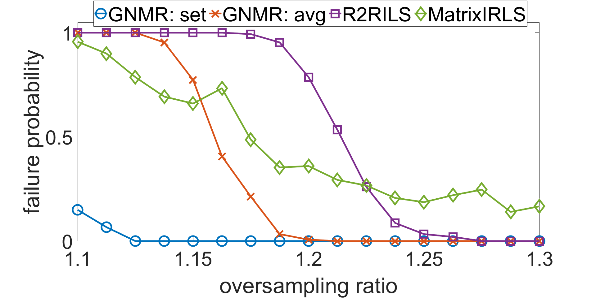
(a)

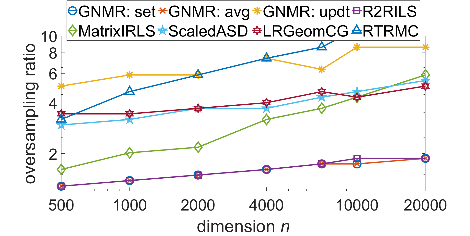
(b)

Figure 5: Same as Fig. 2, but with Y-axes correspond to failure probability, defined as $\text{Pr}[\texttt{rel-RMSE}>10^{-4}]$ (left panel), and lowest oversampling ratio from which the failure probability is smaller than $0.1$ (right panel).

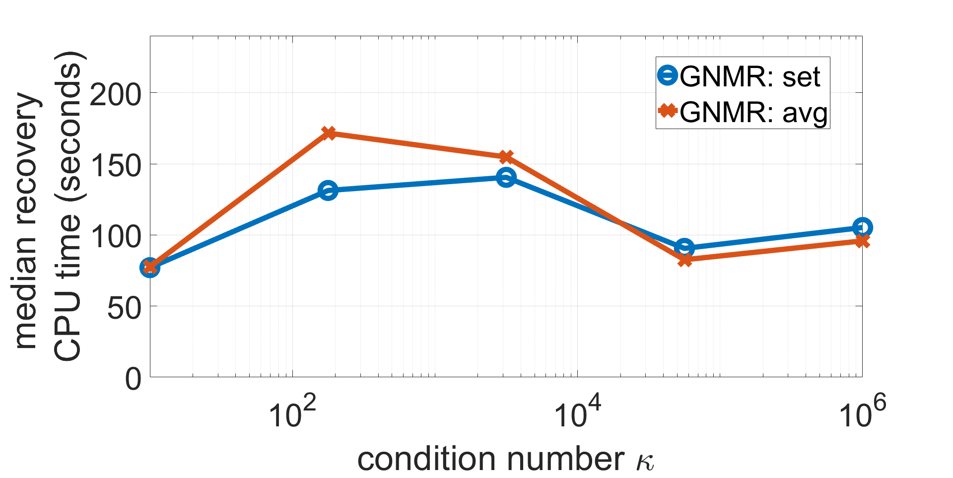
Figure 6: Same as Fig. 3, but with $N^{(2)}_{\text{inner}}=1500$ instead of $200$.

References

- [ABG07] P-A Absil, Christopher G Baker, and Kyle A Gallivan. Trust-region methods on riemannian manifolds. Foundations of Computational Mathematics, 7(3):303–330, 2007.
- [AKKS12] Haim Avron, Satyen Kale, Shiva Prasad Kasiviswanathan, and Vikas Sindhwani. Efficient and practical stochastic subgradient descent for nuclear norm regularization. In Proceedings of the 29th International Conference on Machine Learning, pages 323––330, Madison, WI, USA, 2012. Omnipress.
- [AMS09] P-A Absil, Robert Mahony, and Rodolphe Sepulchre. Optimization algorithms on matrix manifolds. Princeton University Press, 2009.
- [BA15] Nicolas Boumal and P-A Absil. Low-rank matrix completion via preconditioned optimization on the grassmann manifold. Linear Algebra and its Applications, 475:200–239, 2015.
- [BF05] Aeron M Buchanan and Andrew W Fitzgibbon. Damped newton algorithms for matrix factorization with missing data. In Conference on Computer Vision and Pattern Recognition (CVPR), volume 2, pages 316–322. IEEE, 2005.
- [BNZ21] Jonathan Bauch, Boaz Nadler, and Pini Zilber. Rank 2r iterative least squares: efficient recovery of ill-conditioned low rank matrices from few entries. SIAM Journal on Mathematics of Data Science, 3(1):439–465, 2021.
- [BTW15] Jeffrey D Blanchard, Jared Tanner, and Ke Wei. CGIHT: conjugate gradient iterative hard thresholding for compressed sensing and matrix completion. Information and Inference: A Journal of the IMA, 4(4):289–327, 2015.
- [Can08] Emmanuel J Candes. The restricted isometry property and its implications for compressed sensing. Comptes rendus mathematique, 346(9-10):589–592, 2008.
- [CBSW15] Yudong Chen, Srinadh Bhojanapalli, Sujay Sanghavi, and Rachel Ward. Completing any low-rank matrix, provably. The Journal of Machine Learning Research, 16(1):2999–3034, 2015.
- [CCD+21] Vasileios Charisopoulos, Yudong Chen, Damek Davis, Mateo Díaz, Lijun Ding, and Dmitriy Drusvyatskiy. Low-rank matrix recovery with composite optimization: good conditioning and rapid convergence. Foundations of Computational Mathematics, pages 1–89, 2021.
- [CCF+20] Yuxin Chen, Yuejie Chi, Jianqing Fan, Cong Ma, and Yuling Yan. Noisy matrix completion: Understanding statistical guarantees for convex relaxation via nonconvex optimization. SIAM Journal on Optimization, 30(4):3098–3121, 2020.
- [CCS10] Jian-Feng Cai, Emmanuel J Candès, and Zuowei Shen. A singular value thresholding algorithm for matrix completion. SIAM Journal on Optimization, 20(4):1956–1982, 2010.
- [CFMY21] Yuxin Chen, Jianqing Fan, Cong Ma, and Yuling Yan. Bridging convex and nonconvex optimization in robust pca: Noise, outliers and missing data. The Annals of Statistics, 49(5):2948–2971, 2021.
- [CGJ17] Yeshwanth Cherapanamjeri, Kartik Gupta, and Prateek Jain. Nearly optimal robust matrix completion. In International Conference on Machine Learning, pages 797–805. PMLR, 2017.
- [Che15] Yudong Chen. Incoherence-optimal matrix completion. IEEE Transactions on Information Theory, 61(5):2909–2923, 2015.
- [CL19] Eric C Chi and Tianxi Li. Matrix completion from a computational statistics perspective. Wiley Interdisciplinary Reviews: Computational Statistics, 11(5):e1469, 2019.
- [CLC19] Yuejie Chi, Yue M Lu, and Yuxin Chen. Nonconvex optimization meets low-rank matrix factorization: An overview. IEEE Transactions on Signal Processing, 67(20):5239–5269, 2019.
- [CLL20] Ji Chen, Dekai Liu, and Xiaodong Li. Nonconvex rectangular matrix completion via gradient descent without regularization. IEEE Transactions on Information Theory, 66(9):5806–5841, 2020.
- [CP10] Emmanuel J Candes and Yaniv Plan. Matrix completion with noise. Proceedings of the IEEE, 98(6):925–936, 2010.
- [CR09] Emmanuel J Candès and Benjamin Recht. Exact matrix completion via convex optimization. Foundations of Computational mathematics, 9(6):717, 2009.
- [CT10] Emmanuel J Candès and Terence Tao. The power of convex relaxation: Near-optimal matrix completion. IEEE Transactions on Information Theory, 56(5):2053–2080, 2010.
- [DC20] Lijun Ding and Yudong Chen. Leave-one-out approach for matrix completion: Primal and dual analysis. IEEE Transactions on Information Theory, 66(11):7274–7301, 2020.
- [DR16] Mark A Davenport and Justin Romberg. An overview of low-rank matrix recovery from incomplete observations. IEEE Journal of Selected Topics in Signal Processing, 10(4):608–622, 2016.
- [FHB+01] Maryam Fazel, Haitham Hindi, Stephen P Boyd, et al. A rank minimization heuristic with application to minimum order system approximation. Proceedings of the American control conference, 6:4734–4739, 2001.
- [FO05] Uriel Feige and Eran Ofek. Spectral techniques applied to sparse random graphs. Random Structures & Algorithms, 27(2):251–275, 2005.
- [FRW11] Massimo Fornasier, Holger Rauhut, and Rachel Ward. Low-rank matrix recovery via iteratively reweighted least squares minimization. SIAM Journal on Optimization, 21(4):1614–1640, 2011.
- [GJZ17] Rong Ge, Chi Jin, and Yi Zheng. No spurious local minima in nonconvex low rank problems: A unified geometric analysis. In International Conference on Machine Learning, pages 1233–1242. PMLR, 2017.
- [GLM16] Rong Ge, Jason D Lee, and Tengyu Ma. Matrix completion has no spurious local minimum. In Advances in Neural Information Processing Systems, pages 2973–2981, 2016.
- [GP03] Gene Golub and Victor Pereyra. Separable nonlinear least squares: the variable projection method and its applications. Inverse problems, 19(2):R1, 2003.
- [GP10] Victor Guillemin and Alan Pollack. Differential topology, volume 370. American Mathematical Soc., 2010.
- [Gro11] David Gross. Recovering low-rank matrices from few coefficients in any basis. IEEE Transactions on Information Theory, 57(3):1548–1566, 2011.
- [Har14] Moritz Hardt. Understanding alternating minimization for matrix completion. In 2014 IEEE 55th Annual Symposium on Foundations of Computer Science, pages 651–660. IEEE, 2014.
- [HH09] Justin P Haldar and Diego Hernando. Rank-constrained solutions to linear matrix equations using powerfactorization. IEEE Signal Processing Letters, 16(7):584–587, 2009.
- [HW14] Moritz Hardt and Mary Wootters. Fast matrix completion without the condition number. In Conference on learning theory, pages 638–678. PMLR, 2014.
- [JD13] Prateek Jain and Inderjit S Dhillon. Provable inductive matrix completion. arXiv preprint arXiv:1306.0626, 2013.
- [JMD10] Prateek Jain, Raghu Meka, and Inderjit Dhillon. Guaranteed rank minimization via singular value projection. In Proceedings of the 23rd International Conference on Neural Information Processing Systems-Volume 1, pages 937–945, 2010.
- [JN15] Prateek Jain and Praneeth Netrapalli. Fast exact matrix completion with finite samples. In Conference on Learning Theory, pages 1007–1034, 2015.
- [JNS13] Prateek Jain, Praneeth Netrapalli, and Sujay Sanghavi. Low-rank matrix completion using alternating minimization. In Proceedings of the forty-fifth annual ACM symposium on Theory of computing, pages 665–674. ACM, 2013.
- [JY09] Shuiwang Ji and Jieping Ye. An accelerated gradient method for trace norm minimization. In Proceedings of the 26th annual international conference on machine learning, pages 457–464. ACM, 2009.
- [KC14] Anastasios Kyrillidis and Volkan Cevher. Matrix recipes for hard thresholding methods. Journal of mathematical imaging and vision, 48(2):235–265, 2014.
- [Kes12] Raghunandan Hulikal Keshavan. Efficient algorithms for collaborative filtering. Stanford University, 2012.
- [KMO10] Raghunandan H Keshavan, Andrea Montanari, and Sewoong Oh. Matrix completion from a few entries. IEEE transactions on Information Theory, 56(6):2980–2998, 2010.
- [KS18] Christian Kümmerle and Juliane Sigl. Harmonic mean iteratively reweighted least squares for low-rank matrix recovery. The Journal of Machine Learning Research, 19(1):1815–1863, 2018.
- [KV20] Christian Kümmerle and Claudio M Verdun. Escaping saddle points in ill-conditioned matrix completion with a scalable second order method. In Workshop on Beyond First Order Methods in ML Systems at the International Conference on Machine Learning, 2020.
- [KV21] Christian Kümmerle and Claudio M Verdun. A scalable second order method for ill-conditioned matrix completion from few samples. In International Conference on Machine Learning (ICML), 2021.
- [LCZL20] Yuanxin Li, Yuejie Chi, Huishuai Zhang, and Yingbin Liang. Non-convex low-rank matrix recovery with arbitrary outliers via median-truncated gradient descent. Information and Inference: A Journal of the IMA, 9(2):289–325, 2020.
- [LHLZ20] Yuetian Luo, Wen Huang, Xudong Li, and Anru R Zhang. Recursive importance sketching for rank constrained least squares: Algorithms and high-order convergence. arXiv preprint arXiv:2011.08360, 2020.
- [LLA+19] Xingguo Li, Junwei Lu, Raman Arora, Jarvis Haupt, Han Liu, Zhaoran Wang, and Tuo Zhao. Symmetry, saddle points, and global optimization landscape of nonconvex matrix factorization. IEEE Transactions on Information Theory, 65(6):3489–3514, 2019.
- [LLZ+20] Shuang Li, Qiuwei Li, Zhihui Zhu, Gongguo Tang, and Michael B Wakin. The global geometry of centralized and distributed low-rank matrix recovery without regularization. IEEE Signal Processing Letters, 27:1400–1404, 2020.
- [MGC11] Shiqian Ma, Donald Goldfarb, and Lifeng Chen. Fixed point and Bregman iterative methods for matrix rank minimization. Mathematical Programming, 128(1-2):321–353, 2011.
- [MHT10] Rahul Mazumder, Trevor Hastie, and Robert Tibshirani. Spectral regularization algorithms for learning large incomplete matrices. Journal of machine learning research, 11(Aug):2287–2322, 2010.
- [MLC21] Cong Ma, Yuanxin Li, and Yuejie Chi. Beyond procrustes: Balancing-free gradient descent for asymmetric low-rank matrix sensing. IEEE Transactions on Signal Processing, 69:867–877, 2021.
- [MMBS13] Bamdev Mishra, Gilles Meyer, Francis Bach, and Rodolphe Sepulchre. Low-rank optimization with trace norm penalty. SIAM Journal on Optimization, 23(4):2124–2149, 2013.
- [MMBS14] Bamdev Mishra, Gilles Meyer, Silvère Bonnabel, and Rodolphe Sepulchre. Fixed-rank matrix factorizations and Riemannian low-rank optimization. Computational Statistics, 29(3-4):591–621, 2014.
- [MS12] Goran Marjanovic and Victor Solo. On optimization and matrix completion. IEEE Transactions on signal processing, 60(11):5714–5724, 2012.
- [MS14] Bamdev Mishra and Rodolphe Sepulchre. R3MC: A Riemannian three-factor algorithm for low-rank matrix completion. In 53rd IEEE Conference on Decision and Control, pages 1137–1142. IEEE, 2014.
- [MWCC19] Cong Ma, Kaizheng Wang, Yuejie Chi, and Yuxin Chen. Implicit regularization in nonconvex statistical estimation: Gradient descent converges linearly for phase retrieval, matrix completion, and blind deconvolution. Foundations of Computational Mathematics, 2019.
- [NS12] Thanh Ngo and Yousef Saad. Scaled gradients on grassmann manifolds for matrix completion. In Advances in Neural Information Processing Systems, pages 1412–1420, 2012.
- [OD07] Takayuki Okatani and Koichiro Deguchi. On the wiberg algorithm for matrix factorization in the presence of missing components. International Journal of Computer Vision, 72(3):329–337, 2007.
- [OYD11] Takayuki Okatani, Takahiro Yoshida, and Koichiro Deguchi. Efficient algorithm for low-rank matrix factorization with missing components and performance comparison of latest algorithms. In International Conference on Computer Vision, pages 842–849. IEEE, 2011.
- [PABN16] Daniel L Pimentel-Alarcón, Nigel Boston, and Robert D Nowak. A characterization of deterministic sampling patterns for low-rank matrix completion. IEEE Journal of Selected Topics in Signal Processing, 10(4):623–636, 2016.
- [PKCS18] Dohyung Park, Anastasios Kyrillidis, Constantine Caramanis, and Sujay Sanghavi. Finding low-rank solutions via nonconvex matrix factorization, efficiently and provably. SIAM Journal on Imaging Sciences, 11(4):2165–2204, 2018.
- [PS82] Christopher C Paige and Michael A Saunders. LSQR: An algorithm for sparse linear equations and sparse least squares. ACM Transactions on Mathematical Software (TOMS), 8(1):43–71, 1982.
- [PT94] Pentti Paatero and Unto Tapper. Positive matrix factorization: A non-negative factor model with optimal utilization of error estimates of data values. Environmetrics, 5(2):111–126, 1994.
- [Rec11] Benjamin Recht. A simpler approach to matrix completion. Journal of Machine Learning Research, 12(Dec):3413–3430, 2011.
- [RFP10] Benjamin Recht, Maryam Fazel, and Pablo A Parrilo. Guaranteed minimum-rank solutions of linear matrix equations via nuclear norm minimization. SIAM review, 52(3):471–501, 2010.
- [RS05] Jasson DM Rennie and Nathan Srebro. Fast maximum margin matrix factorization for collaborative prediction. In Proceedings of the 22nd international conference on Machine learning, pages 713–719. ACM, 2005.
- [RW80] Axel Ruhe and Per Åke Wedin. Algorithms for separable nonlinear least squares problems. SIAM review, 22(3):318–337, 1980.
- [SC10] Amit Singer and Mihai Cucuringu. Uniqueness of low-rank matrix completion by rigidity theory. SIAM Journal on Matrix Analysis and Applications, 31(4):1621–1641, 2010.
- [SL16] Ruoyu Sun and Zhi-Quan Luo. Guaranteed matrix completion via non-convex factorization. IEEE Transactions on Information Theory, 62(11):6535–6579, 2016.
- [TBS+16] Stephen Tu, Ross Boczar, Max Simchowitz, Mahdi Soltanolkotabi, and Ben Recht. Low-rank solutions of linear matrix equations via procrustes flow. In International Conference on Machine Learning, pages 964–973. PMLR, 2016.
- [TMC21a] Tian Tong, Cong Ma, and Yuejie Chi. Accelerating ill-conditioned low-rank matrix estimation via scaled gradient descent. Journal of Machine Learning Research, 22(150):1–63, 2021.
- [TMC21b] Tian Tong, Cong Ma, and Yuejie Chi. Low-rank matrix recovery with scaled subgradient methods: Fast and robust convergence without the condition number. IEEE Transactions on Signal Processing, 69:2396–2409, 2021.
- [TW13] Jared Tanner and Ke Wei. Normalized iterative hard thresholding for matrix completion. SIAM Journal on Scientific Computing, 35(5):S104–S125, 2013.
- [TW16] Jared Tanner and Ke Wei. Low rank matrix completion by alternating steepest descent methods. Applied and Computational Harmonic Analysis, 40(2):417–429, 2016.
- [TY10] Kim-Chuan Toh and Sangwoon Yun. An accelerated proximal gradient algorithm for nuclear norm regularized linear least squares problems. Pacific Journal of optimization, 6(615-640):15, 2010.
- [Van13] Bart Vandereycken. Low-rank matrix completion by Riemannian optimization. SIAM Journal on Optimization, 23(2):1214–1236, 2013.
- [Wah65] Grace Wahba. A least squares estimate of satellite attitude. SIAM review, 7(3):409–409, 1965.
- [WCCL16] Ke Wei, Jian-Feng Cai, Tony F Chan, and Shingyu Leung. Guarantees of Riemannian optimization for low rank matrix recovery. SIAM Journal on Matrix Analysis and Applications, 37(3):1198–1222, 2016.
- [WCZT21] Yuqing Wang, Minshuo Chen, Tuo Zhao, and Molei Tao. Large learning rate tames homogeneity: Convergence and balancing effect. arXiv preprint arXiv:2110.03677, 2021.
- [Wib76] T Wiberg. Computation of principal components when data are missing. In Proc. Second Symp. Computational Statistics, pages 229–236, 1976.
- [WYZ12] Zaiwen Wen, Wotao Yin, and Yin Zhang. Solving a low-rank factorization model for matrix completion by a nonlinear successive over-relaxation algorithm. Mathematical Programming Computation, 4(4):333–361, 2012.
- [XJZ13] Miao Xu, Rong Jin, and Zhi-Hua Zhou. Speedup matrix completion with side information: Application to multi-label learning. In Advances in neural information processing systems, pages 2301–2309, 2013.
- [YD21] Tian Ye and Simon S Du. Global convergence of gradient descent for asymmetric low-rank matrix factorization. Advances in Neural Information Processing Systems, 34, 2021.
- [YPCC16] Xinyang Yi, Dohyung Park, Yudong Chen, and Constantine Caramanis. Fast algorithms for robust pca via gradient descent. In Proceedings of the 30th International Conference on Neural Information Processing Systems, pages 4159–4167, 2016.
- [YZMCS19] Man-Chung Yue, Zirui Zhou, and Anthony Man-Cho So. On the quadratic convergence of the cubic regularization method under a local error bound condition. SIAM Journal on Optimization, 29(1):904–932, 2019.
- [ZDG18] Xiao Zhang, Simon Du, and Quanquan Gu. Fast and sample efficient inductive matrix completion via multi-phase procrustes flow. In International Conference on Machine Learning, pages 5756–5765. PMLR, 2018.
- [ZL15] Qinqing Zheng and John Lafferty. A convergent gradient descent algorithm for rank minimization and semidefinite programming from random linear measurements. In Proceedings of the 28th International Conference on Neural Information Processing Systems-Volume 1, pages 109–117, 2015.
- [ZL16] Qinqing Zheng and John Lafferty. Convergence analysis for rectangular matrix completion using burer-monteiro factorization and gradient descent. arXiv preprint arXiv:1605.07051, 2016.
- [ZLTW18] Zhihui Zhu, Qiuwei Li, Gongguo Tang, and Michael B Wakin. Global optimality in low-rank matrix optimization. IEEE Transactions on Signal Processing, 66(13):3614–3628, 2018.
- [ZN22] Pini Zilber and Boaz Nadler. Inductive matrix completion: No bad local minima and a fast algorithm. arXiv preprint arXiv:2201.13052, 2022.