Non-diffusive Variational Problems
with Distributional and Weak Gradient Constraints
Abstract.
In this paper, we consider non-diffusive variational problems with mixed boundary conditions and (distributional and weak) gradient constraints. The upper bound in the constraint is either a function or a Borel measure, leading to the state space being a Sobolev one or the space of functions of bounded variation. We address existence and uniqueness of the model under low regularity assumptions, and rigorously identify its Fenchel pre-dual problem. The latter in some cases is posed on a non-standard space of Borel measures with square integrable divergences. We also establish existence and uniqueness of solutions to this pre-dual problem under some assumptions. We conclude the paper by introducing a mixed finite-element method to solve the primal-dual system. The numerical examples confirm our theoretical findings.
Key words and phrases:
non-diffusive variational problems, distributional derivatives, weak derivatives, gradient constraint, Fenchel dual, Borel measure, mixed finite-element method.1. Introduction
We begin by considering an evolutionary problem whose semi-discretization (in time) gives rise to the class of stationary problems of interest in this paper. Suppose that together with are given, where is a bounded domain with a Lipschitz boundary. Furthermore, let be a given nonnegative function (possibly only integrable), or a nonnegative Borel measure in . Suppose that , such that , is a solution to the following problem
| (1.1) |
where the set is given by
| (1.2) |
The choice of and in (1.2) hinges on the type of the boundary conditions and the regularity of . We assume that the boundary is partitioned into a Dirichlet boundary part and a non-Dirichlet boundary part , both composed of a finite number of connected parts, such that
Notice that on , we do not necessarily prescribe Neumann boundary conditions, as it is later clarified. However, a conservation law of material is in place in the case ; specifically, it can be inferred from (1.1) that given that are admissible test functions as we see next. The restriction of to the part of the boundary is assumed to be zero, and no restrictions are assumed on .
The set is convex and it arises by a nonlinear law with a bound on the first order derivative terms. In the most general form is given by
| (1.3) |
with . We briefly discuss the two possible scenarios that we consider:
-
(I)
If is a nonnegative measurable function, then is a Sobolev-type space and is the weak gradient, so that is the -norm of the weak gradient of . Hence, in (1.3) is considered in the almost everywhere (a.e.) in sense.
-
(II)
If is a nonnegative Borel measure, then is a subset of functions of bounded variation . In this case, is the distributional gradient, and the total variation measure of associated to the -norm, and the constraint is understood in the measure sense.
Both instances, (I) and (II) are related, in fact (I) may be considered as a special case of (II). Furthermore, letting in case (II), where denotes the set of nonnegative Borel measures, enables us to handle the delicate case in (I). Next we shall provide a brief description of modeling capabilities of (I) and (II) in the context of a particular application.
A possible motivation for the above class of problems is based on the study of accumulation of granular heterogeneous material on possibly discontinuous structures. This approach was pioneered by Prigozhin [28, 30, 31] in the case of homogeneous materials and a continuous support structure. In this vein, represents the (density) rate of a granular material being deposited on a supporting structure . Moreover, is the total amount of material deposited on over the time interval . In case that is a real number, this corresponds to the classical case of a granular cohesionless material where homogeneous piles are generated. If is not constant zero, the value of at a point determines the angle of repose of the material at that point, i.e., the steepness of a cone generated from a point source of material. This is the case for heterogenous sandpiles [7] and also a restricted case of the quasi-variational sandpile model; see [3, 4, 27, 5]. In a more general setting, where is a measure, using the approach in this paper, it is possible to generate discontinuous structures such as cliffs by preserving discontinuities in the initial supporting structure and/or of . Such an approach has not yet been considered by the literature to the best of our knowledge.
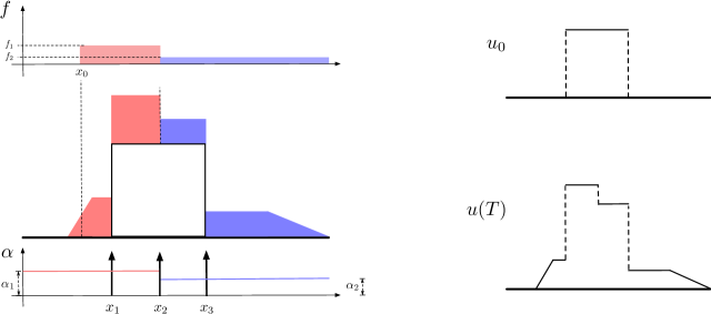
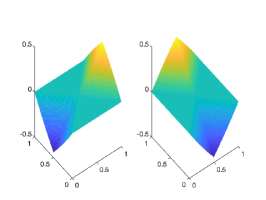
A description of the qualitative behavior of Problem (1.1) is displayed in Figure 1. We assume two materials with different angles of repose and with are poured on the discontinuous structure for and . The intensity of the material being deposited is given by for some points , and , and some , i.e., the first and second materials are poured with density rates and , respectively, during the entire time interval . We further assume that a sharp edge can form at with maximum height of , and in addition discontinuities of maximum size can be preserved at the locations of the discontinuities of . Finally, the the gradient constraint is then given by , and the material is assumed to escape freely at the boundary points of . On the right side of Figure 1, we see the comparison between and , the solution at time ; on the left we see the depiction of , , and the accumulation regions of both materials.
The study of solutions to (1.1) usually makes use of the semi-discretization (in time) of the problem via an implicit Euler method. In particular, we approximate the partial time derivative by for some time-step . The class of problems of interest in this paper is then given by
| () |
Notice that () can be seen as the time-discrete version of (1.1) where the solution to () is equal to when corresponds to with given. Closely related to the problem above, we consider the following class of problems
| () |
We prove that () is the Fenchel pre-dual of problem (), i.e., the Fenchel dual [14] of () under certain conditions is (). Several choices for and are explored which are directly related to the nature of . In all cases considered, contains -dimensional vector fields with divergences in . In particular, we consider
-
(i)
If is a nonnegative measurable function (additional assumptions are later explained but continuity is enough to guarantee what follows), then we explore two options for :
In the first case is a subspace of . In the second case is contained in the space of -valued Borel measures, so that the second functional denotes the integral of with respect to the total variation measure of induced by the -norm. The two functionals are closely related, and the first can be seen as a restriction of the second one to measures that are absolutely continuous with respect to the Lebesgue measure.
-
(ii)
If is a nonnegative Borel measure, then is contained in the space of maps that are measurable, with given by
A few words are in order concerning () and (). Although the objective functional in () is smooth and amenable, the constraint set makes the entire problem highly nonlinear and nonsmooth. The latter also holds for () given the nature of the functional . The development of solution algorithms for both problems is a rather delicate issue that requires appropriate regularization methods that can handle the nonsmothness in an asymptotic fashion.
The paper focuses on functional analytic properties of () and () together with duality relationship properties. Additionally, we develop a mixed finite type method to solve the optimality conditions corresponding to () and ().
Some Bibliography
The structure of Problems () and () and their inherent difficulties are analogous to the ones that appear in the context of plasticity; see [25, 35] and references therein. In particular, the first class of applications for diffusive variational problems with gradient constraints is the elasto-plastic torsion problem. Such a problem has been thoroughly analyzed by Brézis, Caffarelli, Evans, Friedman, Gerhardt, and others; see [16, 15, 8, 18, 17, 10, 11, 9]. Further, a complete account of the literature can be found in [33]. A significant amount of the aforementioned works focuses on regularity of solutions, the free boundary, and the equivalence of the gradient constrained problem to a double obstacle one.
The modeling of the evolution of the magnetic field in critical-state models of type-II superconductors also leads to a problem like (1.1) with the addition of a diffusive operator and a state-dependent constraint in some cases; see [32, 2, 29, 30, 20, 23, 21]. See [34] for a study of evolutionary variational problems with non-constant gradient constraints, and [26] for a complete account of evolutionary problems with derivative bounds.
Analogous problems are found in mathematical imaging involving total variation regularization [24, 19, 6] and more specifically in the weighted total variation version [22]. There, in contrast to the work here, the -norm on the gradient is replaced by the -norm, leading to a pre-dual problem with a pointwise bound in its state variable.
1.1. Organization of the paper.
Preliminaries are provided, and some notations are made explicit in Section 2; elementary results about the generalized gradient constraint are given in Section 2.1. In Section 3, we prove existence and uniqueness of the solution to problem () for the cases when is either a nonnegative Lebesgue measurable function or a nonnegative Borel measure. Existence of solutions to problem () is addressed in Section 4, while for the case when is a function we require , when is a measure the dimension restriction is dropped. The relation between problems () and () are considered in Section 5, where a rigorous Fenchel duality result establishes a link between these two problems. In particular, in Section 5.1, we address the case where is a function and the variable is either a function or a measure. The case when is a measure and an extension of the duality result of the previous section is given in Section 5.2. Finally in Section 6, we introduce a mixed finite element method to solve the underlying problems and present a range of numerical tests.
2. Notation and Preliminaries
The purpose of this section is to introduce notation involving spaces, and convergence notions that are used throughout the paper; in particular, we address the well-known notions of Sobolev spaces and the space of functions of bounded variation. We refer the reader to Attouch et al. [12] that we follow closely for this introduction together with the book of Adams and Fournier [1].
For a Banach space , we denote its corresponding norm as . For an element in the topological dual of , the duality pairing of and an arbitrary element is written as . Throughout the paper, all Banach spaces are assumed to be real vector spaces.
The inner product on the Lebesgue space of (equivalence classes of) functions that are square integrable on is denoted as , so that for where refers to integration with respect to the Lebesgue measure.
The Sobolev space of functions in for with weak gradients in is denoted by , and it is endowed with the norm
where denotes the weak gradient of . In the case , we use the notation . Given that is assumed Lipschitz, restriction of a function to the boundary is well-defined via the continuous trace map . Furthermore, the closed subspace of functions in that are zero on is denoted by , i.e.,
Similarly, we define .
The space of real-valued Borel measures is endowed with the norm , where is defined for an arbitrary open set as
Note that , and that defines a Borel measure in , the subset of non-negative elements of , i.e., if for every Borel set .
We denote by , the space of functions in , for which the total variation semi-norm
is finite and where is the Hölder conjugate of , i.e., ; see [12, Section 10.1]. The space is a Banach space endowed with the norm
The operator represents the distributional gradient, and for a , is a -valued Borel measure. We use to denote the total variation measure (associated to the -norm) of , and the total mass is by definition
Furthermore, the Lebesgue decomposition result applied to implies that there exist measures and such that
with and respectively being absolutely continuous and singular with respect to the -dimensional Lebesgue measure.
We define now the notions of weak and intermediate convergence of sequences in which provide different topologies on the space . The former is obtained by a subsequence of a bounded sequence in . Moreover, the latter is sufficient to preserve boundary conditions in the sense of the trace as stated in Theorem 2.3 below.
Definition 2.1 (Weak convergence for ).
Let be a sequence in and . We say that converges to weakly, denoted as in , if
Recall that if is a sequence of measures in then in for some , that is, weakly converges to , if
for all .
The definition 2.1 is understood in light of the following fact: If is a bounded sequence in , there exists such that along a subsequence in . The latter follows since the embedding is compact (see Attouch et al. [12, Theorem 10.1.4.]) for Lipschitz domains, and since a bounded sequence of measures admits a weakly convergent subsequence.
We shall use the direct method of calculus of variations to establish existence of solutions to problems in and with Dirichlet homogeneous boundary conditions on . The space of interest is defined as
where is a trace operator; see [12, section 10.2]. Notice that we use the same notation for the trace operator in Sobolev spaces . There is a fundamental issue with the trace in and the application of the direct method as we show next with an standard example adapted from [12].
Consider a bounded sequence in . Then, we can extract a subsequence (not relabeled) of such that in . The problem is that in general it is not possible to say that : Let with , and consider defined as
Then, , and , with . The underlying reason is that the trace operator in is not continuous with respect to weak convergence, but it is with respect to the intermediate convergence subsequently defined. We further notice that and , this discrepancy is central to the issue we are considering.
Definition 2.2 (Intermediate convergence).
Let be a sequence in and . We say that converges to in the sense of intermediate convergence if
The name intermediate convergence arises since it describes a stronger topology than the one of weak convergence, but not as strong as the norm one. The importance of the intermediate convergence can be seen in the following result which holds in our case since is a Lipschitz bounded domain. We refer to Attouch et al. [12, Theorem 10.2.2] for its proof.
Theorem 2.3.
The trace operator is continuous when is equipped with the intermediate convergence and when is equipped with the strong convergence.
We also note that is dense in in the intermediate convergence topology, for a proof see [12, Theorem 10.1.2].
2.1. The gradient constraint
A few words are in order concerning the gradient constraint given in the set defined in (1.3). Although in the case when the situation is somewhat standard, if , the distributional gradient for BV functions, require several non-trivial explanations. In the cases where is a Borel measure and , the inequality
| (2.1) |
in (1.3) is understood in the sense of measures, i.e., (2.1) holds true if
| (2.2) |
and equivalently, for every Borel measurable set , it holds that
| (2.3) |
Given that nonnegative Borel measures are inner and outer regular ([12, Proposition 4.2.1]) the condition (2.2) is equivalent to
| (2.4) |
for all open sets .
It is possible to replace in (2.2) by , which we discuss next.
Proposition 2.4.
The condition in (2.2) is equivalent to
| (2.5) |
Proof.
Suppose that (2.2) holds true and let be a sequence of closed sets such that
| (2.6) |
The sequence exists given that measures in are inner regular; see [12, Proposition 4.2.1]. Let be nonnegative and arbitrary.
Accordingly, let in be nonnegative, uniformly bounded in , and such that in . Hence can be uniformly estimated by a constant, and by (2.6) it holds that
Since the inequality in (2.5) holds for every by initial assumption, it also holds in the limit for . Furthermore, (2.5) immediately implies (2.2), so the result is proven. ∎
3. Existence Theory for
In this section, we discuss the existence and uniqueness of solution to the problem eq. . We start with the case when is a measure, and the case when is a function follows as a special one. In particular, existence of solutions is studied in the function spaces and . Both of these spaces share the same difficulty: Bounded sequences do not necessarily admit convergent (in some sense) subsequences that preserve the zero boundary condition on in the limit. The main purpose of this section is to overcome this obstacle.
3.1. The case when is a nonnegative Borel measure
We consider in this section that and hence the state space is given by
We start by proving the following lemma which gives sequential precompactness of some classes of bounded sets in . These bounded sets are subsets of which in this case is defined as
Lemma 3.1.
Let , then the set
is sequentially precompact in the sense of the intermediate convergence of for any .
Proof.
Let be a sequence in , then it is bounded in , and thus in for some along a subsequence (not relabelled). Since in , and it follows that for every open set that
| (3.1) |
where we have used the lower-semicontinuity property for open sets of weak convergence of measures; see [12, Proposition 4.2.3]. Additionally, since elements in are outer (and inner) regular, we have that for a Borel set it holds that where the infimum is taken over all open sets such that ; see [12, Proposition 4.2.1]. Thus,
| (3.2) |
follows from (3.1) by taking the infimum over .
In order to prove that converges to in the sense of intermediate convergence, we are only left to prove that narrowly in (see [12, Proposition 10.1.2]). The latter meaning that for each continuous and bounded on . Given that we have that for each there exists a compact set such that
Since , then , and hence for each the compact set , is such that
Then, by Prokhorov Theorem (see [12, Theorem 4.2.3]), there is a subsequence of (not relabelled) that narrowly in . That is, along a subsequence, converges to in the sense of intermediate convergence. This implies that
by virtue of Theorem 2.3 and the fact that for all . ∎
The above results particularly means that for a sequence in that is bounded in , there exists a subsequence that converges to some in the sense of intermediate convergence. Further, and also . A direct consequence of the above lemma is the following result.
Proof.
Consider an infimizing sequence for (). It follows that is bounded in and hence Lemma 3.1 is applicable. That is, there is a subsequence of (not relabelled) such that in , and in the sense of the intermediate convergence for , and further . Finally, by exploiting the weakly lower semicontinuity property of the objective functional in (), we have that is a minimizer. ∎
Next we discuss the case when is a function.
3.2. The case when is an integrable function
In this section, we let be a nonnegative and integrable function, leading to
This case can be interpreted (to some extent) as a special case of the one in the previous subsection under the assumption that is a measure absolutely continuous with respect to the Lebesgue measure. However, we proceed in a slightly different fashion by considering as a function and the state space contained in ; this provides further insight on bounded sequences in and in Sobolev spaces. In this case, we have given by
Next we state a version of Lemma 3.1 adapted to the current setting which can be used to prove existence of solutions to ().
Lemma 3.3.
Let and , then every sequence in the set
admits a subsequence satisfying
for some , which is also the weak limit in of the same subsequence.
The above can be seen as a consequence of equi-integrability of the set . Recall that a family of functions is equi-integrable provided that for every , there exists a such that for every set with we have that for all Further, the Dunford-Pettis theorem states that if is a bounded sequence in and is equi-integrable, then along a subsequence for some . Hence, since is bounded in , and the gradients are equi-integrable, it is simple to infer strong convergence in together with weak convergence of the gradients in . The improvement of the latter convergence is done again via Prokhorov’s result as in the proof of Lemma 3.1 leading to an equivalent of the intermediate convergence in . The trace preservation follows directly from the same proof. Further note that the convergence determined does not imply strong convergence in since this space is not uniformly convex. Another formulation of the above lemma is that bounded sets with equi-integrable gradients are compact in when endowed with the metric
With the use of Lemma 3.3 and following the same argument as before for Theorem 3.2, we have
4. Existence Theory for the pre-dual problem
The focus of this section is on existence and uniqueness of solutions of problem () under different functional analytic settings. In particular, we focus on two cases where is either (i) a function or (ii) a Borel measure. In the first case, we let be either a function or a measure; here, existence results are limited to . On the other hand, in the second case we establish an existence and uniqueness result for with arbitrary , for a specific class of ’s (to be specified later). Furthermore, this second case requires a nonstandard space of vector measures with divergences in . Remarkably, a version of the integration-by-parts formula still holds in this general setting; such a construct is rather recent [37]. We start with the case when is a function.
4.1. The case when is a function and is either a function or a measure
We begin this section by considering that and is defined as
| (4.1) |
Moreover, we define
for .
We assume that if and then is not identically zero, and if then a.e. in . Thus, the space is defined by
| (4.2) |
where
It follows that is a Banach space: If , the result is clear given that a.e. in . If , then which follows from the fact that is an equivalent norm (to the usual one) on . The latter is due to being a seminorm in and norm on the constants, i.e. for , iff ; see [36, Chapter 1.4]. We can now establish existence of a solution to problem eq. .
Theorem 4.1.
Proof.
The proof is based on the direct method. Let be the objective function in eq. , that is,
and let in be an infimizing sequence of . Note that is a norm in ; see [36, Chapter 1.4]. Hence, is bounded in , and there exists a weakly convergent (not relabeled) subsequence such that in . By the compact embedding of (see [1, Chapter 6]) we have existence of a subsequence (not relabeled) in . Finally, weak lower semicontinuity of yields that is a solution to eq. . The strict convexity of the objective functional provides uniqueness to the solution. ∎
An analogous approach can be considered when is a non negative Borel measure (and not identically zero), that is, when . In particular, we set
| (4.3) |
and we construct the space in the same way as in eq. 4.2, but with the norm defined as
and assuming that if and then is not identically zero, and if then if and is a Borel set.
The existence result of Theorem 4.1 follows mutatis mutandis: Since is again a norm in , see [36, Chapter 1.4], the exact argument is applicable in this case.
We can now focus on the case when is a measure which provides a general setting for the problem of interest in terms of existence, uniqueness, and duality results.
4.2. The case when is a function and is a measure
We focus now on problem () when is defined as
| (4.4) |
and is a Borel measure. Notice that the above functional can be seen as a generalization of the functional in (4.1). The latter can be obtained by letting be absolutely continuous with respect to the Lebesgue measure.
The functional analytic setting in this section, requires to be a measure with divergence of in , and to be measurable with respect to . We start with a proper definition of such spaces and their properties. We disregard the possible “boundary conditions” for the variable , so that and we define as follows:
| (4.5) |
where corresponds to the -valued Borel measures in . Specifically, if there exists such that
| (4.6) |
and we define . The space is a Banach space when endowed with the norm
| (4.7) |
where and
Note that above is the duality pairing between and , and hence
Similarly to the definition of , we can define for any open set , and subsequently for an arbitrary Borel set . Hence, induces a nonnegative measure (the total variation measure of ); in addition . Note that the space contains regular maps, clearly if then , in this case “” where is the Lebesgue measure.
A note on the space is in order. Although one may be inclined to think that vector fields whose divergences are in would always have better regularity than just the measure type, this is not true. We consider an example developed by Šilhavý [37] to show otherwise. Let with , and define with with the distributional (measure valued) gradient of ; it follows that . This can be seen as follows: is dense (in the sense of the intermediate convergence) in , this means in particular that for such a smooth sequence defined as with . Since also , the result follows by taking the limit and from (4.6).
Following Šilhavý [37], we have a form of integration-by-parts formula together with a trace result. We denote by the space of Lipschitz maps for and endow it with the norm
where is the Lipschitz constant of on . It follows that for each there exists a linear functional such that for all we have
| (4.8) |
Further, is bounded in the following sense
for some , and all and all . Provided that and have enough differential regularity, we observe
as expected. Thus, (4.8) is an extension of the usual integration-by-parts formula.
We are now ready to state and prove the existence and uniqueness result for problem () under the setting above.
Theorem 4.2.
Proof.
Note first that is well-defined given that is measurable with respect to all Borel measures. Consider an infimizing sequence . Since , then is bounded in . Hence, we can extract a subsequence (not relabelled) such that in for some and in for some . Furthermore, for arbitrary
so that , i.e., .
Since the map is weakly lower semicontinuous, in , and for , we have that is a minimizer by a weakly lower semicontinuity argument. Uniqueness follows from the strict convexity of the objective functional. ∎
At this point, one would be tempted to extend the result to the case where , for example, by defining
| (4.9) |
While the space above is well-defined, it is not clear if the weak limits of sequences in the space also belong to it. In fact, if is bounded, then
for each . However, the weak limit along a subsequence argument is not enough to pass to the limit in the left hand side given that is not necessarily of compact support. This remains an open problem.
5. Duality relation between and
In this section, we discuss the dual problem corresponding to eq. . We start with the case when is a Lebesgue measurable function and further subdivide it into two subsections. In Section 5.1 we discuss the case when the pre-dual variable is a function and in the following Section 5.1.2 we assume that the variable is a measure. Next in Section 5.2, we consider the case where is a measure and the pre-dual variable is a function. In general, we prove that
| Problem () is the Fenchel dual of Problem (). |
In order to keep the discussion self-contained, we introduce the following notation and terminology. For an extended real valued function over a Banach space , by we denote its convex conjugate, which is defined by (e.g. see [14, p. 16])
| (5.1) |
Provided that the operator is defined for a Banach space , and it is bounded, its adjoint is well-defined and is given by for all and all .
5.1. The case when is a function
We first consider the case where is a non negative Lebesgue measurable function and we accordingly set
in eq. for the cases when is a function or a measure, respectively. For each of the choices of above, we will also establish the strong duality to eq. . We assume throughout this section (and for the sake of simplicity) that
for all as discussed in Section 1, together with
and hence,
Note that in Section 3 we proved the existence and uniqueness of solution to Equation .
We compute the dual problem to eq. and show that it is given by problem (). Defining by
| (5.2) |
the problem eq. can be written as
| (5.3) |
for , where the space is chosen based on whether is a function or a measure.
By [14, p. 61], the Fenchel dual of () with respect to the perturbation function
is given by
| (5.4) |
where the convex conjugates , of and are defined according to (5.1), see also [14, p. 17] for more details.
5.1.1. Duality when is a function
Now we show that the problem () is the dual to problem (). In this section, we assume that is given by (4.2), and that
We start by proving the following result:
Theorem 5.1.
For every , it holds that .
We break the proof of the above theorem into Lemmas 5.3 and 5.4, which we state after the following observation.
Remark 5.2.
Observe that only takes the value or : By the definition of the convex conjugate , for any it holds that
| (5.5) |
If , i.e. there exists a such that
we can scale by an arbitrarily large leading to .
Lemma 5.3.
Let with . Then the following hold true:
-
(i)
;
-
(ii)
;
-
(iii)
and ;
-
(iv)
on
and therefore .
Proof.
-
(i)
First we show that implies .
Suppose . Then, since , we have that
(5.6) Then, by using definition of a function of bounded variation, see [12, Definition 10.1.1], we have that the supremum on the right hand side of the above inequality is if and hence, if .
-
(ii)
As , we have that and the inequality is understood in the sense of eq. 2.4. Hence, if
(5.7) for an arbitrary open set , then the required condition immediately follows.
By the assumption , and using integration by parts, we observe that
where the last inequality follows using the definition of and eq. 5.7.
-
(iii)
By (i) and (ii), it holds that
(5.8) for every Borel set (see (2.3)), and especially for every Borel set of Lebesgue measure zero, it follows that vanishes on every set of measure zero, and hence is absolutely continuous w.r.t. the -dimensional Lebesgue measure, and therefore , i.e., the distributional gradient is a weak gradient. Thus, .
-
(iv)
To obtain the boundary conditions on , we will show that if , then .
Subsequently for all , we arrive at
(5.9) To get (5.9), for a , choose such that
then for , we obtain that
Now for , by inner regularity [13, pp. 95, proposition 15.1], there exist closed subsets and such that
Then, by Urysohn’s lemma there exists satisfying, such that
Then for any , applying (5.9) to , we obtain that
Further, from
we infer that
Next, using the two inequalities above in conjunction with
and
we obtain that
Now since and have been chosen arbitrarily, it follows that
This immediately leads to the required result, a.e. on , and the proof is complete.
∎
Finally, the converse result remains to be shown, i.e., if , then ; we prove this next.
Lemma 5.4.
If , then .
Proof.
Since , therefore by the definition of , it holds that and a.e. in . Next, using the definition of the convex conjugate of , we obtain that
| (5.10) |
Next, by using the density of in , from (5.10), we obtain that
Thus, since is non-negative (we can set in the definition of ), it follows that and the proof is complete. ∎
Next we compute the conjugate function of the function .
Proposition 5.5.
The conjugate function of defined in (5.2) is given by
| (5.11) |
Proof.
The proof is an immediate consequence of the definition of . Recalling the definition of and rearranging the terms, we obtain that
The result then follows from elementary calculus. ∎
Proposition 5.6 (Strong duality).
Proof.
As a corollary to Theorems 5.1 and 5.5, it immediately follows that the dual of problem () which is given in eq. 5.4 is identical to problem (). Using that and are convex and continuous proper functions and bounded from below, equality (5.12) and the extremality relation (5.13) follow from the application of Theorem III.4.1 and Proposition III.4.1 in [14, p. 59] in its decomposed form, which is described in Remark III.4.2 therein, where condition (4.20) is satisfied by any . ∎
Remark 5.7.
The duality between () and () holds symmetrically, i.e. () is the dual to problem () as well. Defining the perturbation function by following the framework in [14, pp. 58–60], () can be written as
and the application of [14, (4.20) in p. 61] yields that is convex, l.s.c., proper, and bounded from below, given that the same holds true for and . Thus, it follows from [14, p. 49] that and that () is identical to its bidual problem
i.e., to the dual problem to (), with respect to the perturbation function .
Note that though we assume , results within this section hold for . However recall that the existence result for this case (c.f. Section 4.1) only stands in the case .
5.1.2. Duality when is a measure
We consider now the duality result in the framework of the variable in the space of Borel measures with divergences. Surprisingly, the dual problem remains the same. We recall in this framework that
as in (4.5), and . Since we already assumed that is positive, existence of a unique solution follows from Theorem 4.2.
We again propose to follow the Fenchel dual approach and let and be
In this setting, it also holds that for every , we have , i.e., Theorem 5.1. In fact, we show that Lemma 5.3 and Lemma 5.4 remain true under the functional analytic setting of this section.
Proof of Lemma 5.3.
-
(i)
By choosing with and , we obtain the same inequality as (5.6). Moreover, by following similar steps as before, we can show that
-
(ii)
The proof follows identically as before by considering with .
-
(iii)
The same proof applies.
-
(iv)
Note that a.e. implies that , given that . As shown before, in Remark 5.2, implies which yields for with the following
and the proof follows identically leading to .
∎
Proof of Lemma 5.4.
Let , then from the definition of , it follows that and . Furthermore,
i.e., it follows that . The proof is complete. ∎
From Theorem 5.1, it follows that the duality result of Proposition 5.6 also holds in this setting; the proof is straightforward.
5.2. The case when is a measure
In this section, we will extend the duality result of Proposition 5.6 by letting to be a non negative Borel measure, that is, . However, is a function in this setting. In its more general form, in problem (), we set
| (5.14) |
The results in this subsection are a generalization of the case of the Lebesgue integrable constraint , that was presented in Section 5.1. We shall assume that , see eq. 4.2 for the definition of .
Since , as we discussed in Section 1, we let
| (5.15) |
the distributional gradient, and hence
We prove that the dual problem to () is given by eq. with inequality constraint being understood in the sense of eq. 2.5.
Recall that in section 3 we have shown existence and uniqueness of solution to Equation . Here, we show that dual of problem () is given by (). We start by writing eq. as
with as in (5.14) and , as before, given by
We prove now that Theorem 5.1 holds also true in the current setting. For brevity, we only discuss the essential modifications needed in Lemmas 5.3 and 5.4.
Proof of Theorem 5.1.
This proof follows along the same lines as the proof to Theorem 5.1. We start by observing that the discussion in Remark 5.2 holds in the current setting as well, i.e., only takes the values and . We now prove the result.
Finally, note that it follows identically as before that the polar function of is given by
| (5.16) |
Hence, the duality result of proposition 5.6 also holds in the case where is a measure, with replaced by .
6. A Finite Element Method with Applications
The purpose of this section is to illustrate the applicability of the proposed primal-dual approach to solve Problems () and eq. . We assume throughout this section that .
Recall that Problem () in the case that is given by
| (6.1) |
and that the pre-dual problem eq. is given by
| (6.2) |
Now the first order (necessary and sufficient) optimality condition corresponding to (6.2) in the strong form is given by: Find satisfying
| (6.3) | ||||
where denotes the subdifferential operator. In order to solve (6.3), recall from the extremality conditions (5.13), that if and are solutions to (6.1) and (6.2), respectively, they satisfy
| (6.4) |
Then, a primal-dual system arises from (6.3) and (6.4), which in the weak form becomes the following variational inequality of second kind: Find such that
| (6.5) | |||||
| (6.6) |
Due to their nonlinear and nonsmooth nature, it is challenging to solve (6.5)–(6.6).
We shall proceed by introducing the Huber-regularization for in the last term under the integral in (6.2). This regularization is with piecewise differentiable first order derivative. Therefore one can use Newton type methods to solve the resulting regularized system. For a given parameter , the Huber regularization of is given by
As , . Moreover, is continuously differentiable with derivative given by
Replacing in (6.2) by , the regularized primal-dual system corresponding to (6.5)–(6.6) is given by
| (6.7) | |||||
| (6.8) |
Notice, that is piecewise differentiable and the second order derivative is given by
where is the identity matrix.
6.1. Finite Element Discretization
We discretize and using the lowest order Raviart-Thomas () and piecewise constant finite elements, respectively. Whenever needed, the integrals are computed using Gauss-quadrature which is exact for polynomials of degree less than equal to 4. For each fixed , we solve the discrete saddle point system (6.7)–(6.8) using Newton’s method with backtracking line-search strategy. We stop the Newton iteration when each residual in -norm is smaller than . Each linear solve during the Newton iteration is done using direct solve. Starting from , a continuation strategy is applied where in each step we reduce by a factor of 1.30 until is less than equal to . We initialize the Newton’s method by zero. To compute solution for next , we use the solution corresponding to previous as the initial iterate for the Newton’s method.
6.2. Numerical Examples
Next, we report results from various numerical experiments. In all examples we consider and we assume that , , and hence pure Dirichlet boundary conditions on on the entire boundary are set. In the first example, we construct exact solutions when and are constants. We compare these exact solutions with our finite element approximation. These experiments validate our finite element implementation for constant and and provide optimal rate of convergence. Additionally, we solve () and () first for a fixed and vary and next we fix and vary . In our second experiment, we consider a more generic with different features such as cone, valley and flat regions. In our final experiment, we consider to be a measure.
Example 1.
Note initially that if and are constants, it is possible to calculate an exact solution. By setting
the exact and are given as:
and
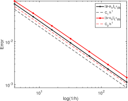
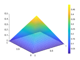
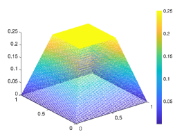
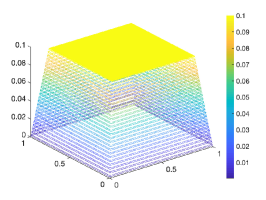
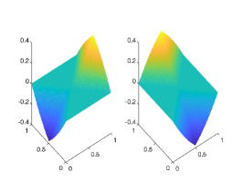
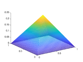
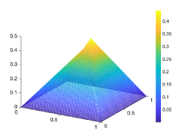
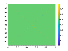
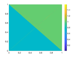
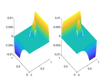
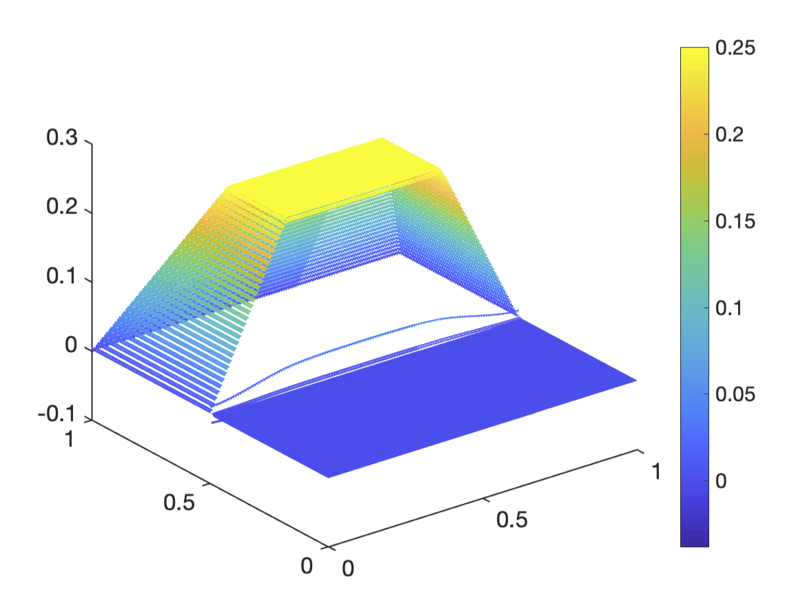
Notice that in this example, is again Lipschitz continuous. In Figure 2 (top panel), we have shown the and when , , and . We observe optimal rate of convergence in both cases. In the bottom row, the left panel shows , the middle panel shows , and the right panel shows . We observe that, in this example, the gradient constraints are active in the entire region. Notice, that at the corners (which are sets of measure zero), gradient is undefined.


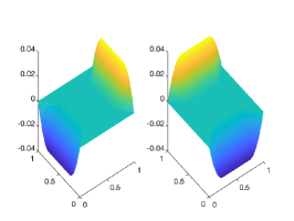
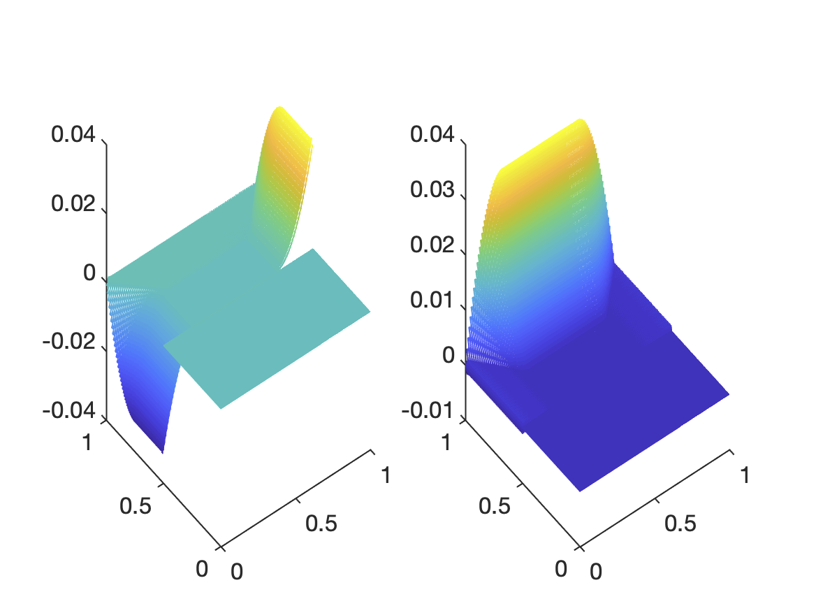
Next, we fix the number of and unknowns to be 197,120 and 131,072, respectively. Figure 3 shows our results for 3 different experiments. In all cases, we have used a fixed . The rows correspond to , and . Each column correspond to , , and . As expected, for a large value of , we observe steep slope, but for smaller values of , plateau regions appear. We also observe that the active region shrinks as decreases since the gradient is zero at the top of the plateau. The dual variable also changes significantly with .

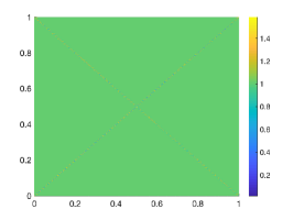
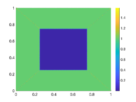
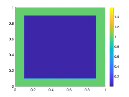
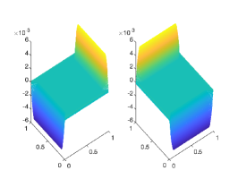
In Figure 4 we again show results from 3 different experiments. In all cases, we have used a fixed . The rows correspond to , and . Each column corresponds to
respectively. In all cases, we observe that the gradient constraints are active in the entire domain (except on a set of measure zero). For the case of piecewise constant , nonsmoothness in is clearly visible.
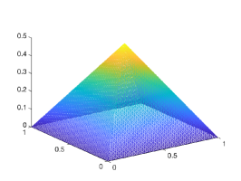


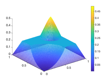
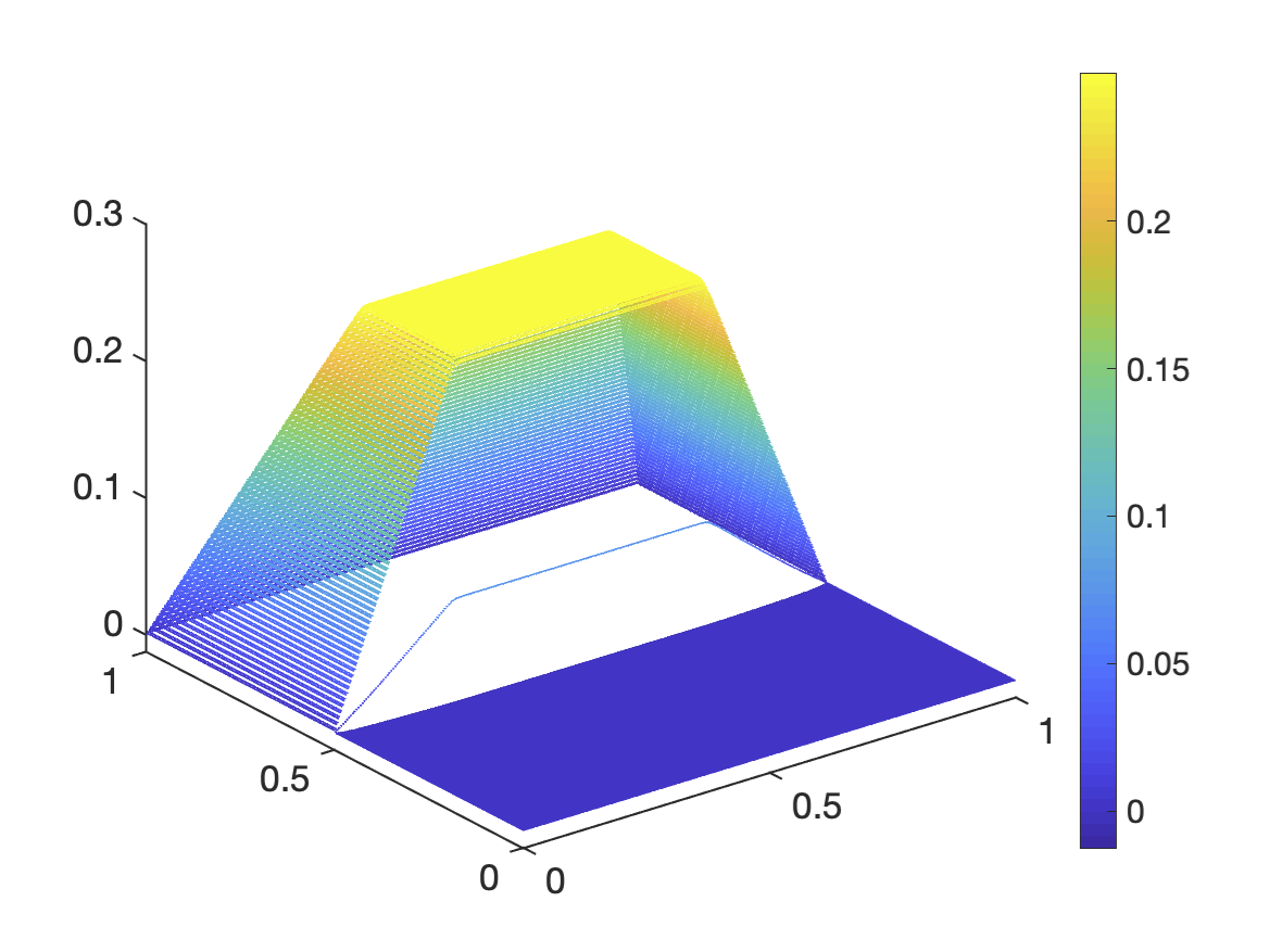
Example 2.
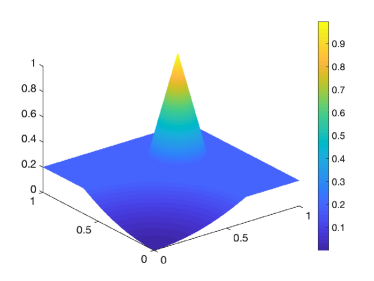
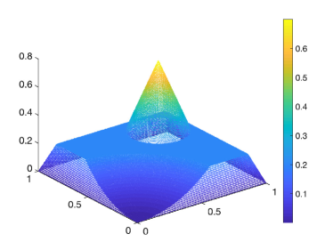
Figure 5 (right panel) shows the computed solution . In Figure 6, we have shown (left panel), and (right panel). Notice that, the gradient constraints are active. Moreover, we also observe significant flat regions, where the gradient is zero.
In Figure 7 have also displayed , and when .
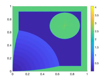
Example 3.
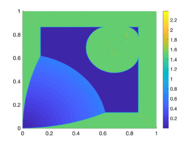
In this example, we consider given by
The main novelty and challenge in this example is the fact that we let to be a measure. Specifically
for all and where , i.e., consists in the Lebesgue measure and a weighted line measure on .
Let denotes the meshsize, then is approximated as
where
As , we approximate the measure in the sense that for all .
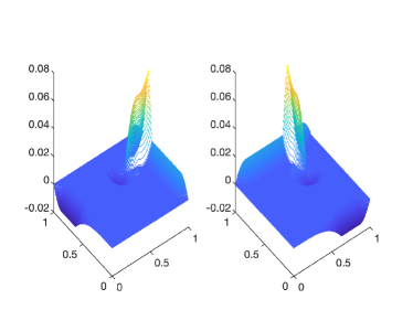
When , the results are shown in Figure 8 (top row). Finally, when the results are provided in Figure 8 (bottom row). We notice that as , we indeed approximate the measure: In fact, we observe a clear discontinuity on the solution , the size of the jump is below which is the upper bound on the distributional gradient on .

References
- [1] R. A. Adams and J. J. F. Fournier. Sobolev spaces, volume 140 of Pure and Applied Mathematics (Amsterdam). Elsevier/Academic Press, Amsterdam, second edition, 2003.
- [2] J. W. Barrett and L. Prigozhin. A quasi-variational inequality problem in superconductivity. Math. Models Methods Appl. Sci., 20(5):679–706, 2010.
- [3] J. W. Barrett and L. Prigozhin. A quasi-variational inequality problem arising in the modeling of growing sandpiles. ESAIM Math. Model. Numer. Anal., 47(4):1133–1165, 2013.
- [4] J. W. Barrett and L. Prigozhin. Lakes and rivers in the landscape: a quasi-variational inequality approach. Interfaces Free Bound., 16(2):269–296, 2014.
- [5] J. W. Barrett and L. Prigozhin. Sandpiles and superconductors: nonconforming linear finite element approximations for mixed formulations of quasi-variational inequalities. IMA J. Numer. Anal., 35(1):1–38, 2015.
- [6] S. Bartels and M. Milicevic. Iterative finite element solution of a constrained total variation regularized model problem. Discrete & Continuous Dynamical Systems-S, 10(6):1207, 2017.
- [7] M. Bocea, M. Mihăilescu, M. Pérez-Llanos, and J. D. Rossi. Models for growth of heterogeneous sandpiles via mosco convergence. Asymptotic Analysis, 78(1-2):11–36, 2012.
- [8] H. Brezis and M. Sibony. Équivalence de deux inéquations variationnelles et applications. Archive for Rational Mechanics and Analysis, 41(4):254–265, 1971.
- [9] H. Brezis and G. Stampacchia. Sur la régularité de la solution d’inéquations elliptiques. Bull. Soc. Math. France, 96:153–180, 1968.
- [10] L. A. Caffarelli and A. Friedman. The free boundary for elastic-plastic torsion problems. Trans. Amer. Math. Soc., 252:65–97, 1979.
- [11] L. A. Caffarelli and A. Friedman. Unloading in the elastic-plastic torsion problem. J. Differential Equations, 41(2):186–217, 1981.
- [12] A. Chambolle. Variational analysis in Sobolev and BV spaces. Applications to PDEs and optimization. Second edition [book review of MR3288271]. SIAM Rev., 58(4):800–802, 2016.
- [13] E. DiBenedetto. Real analysis. Birkhäuser Advanced Texts: Basler Lehrbücher. [Birkhäuser Advanced Texts: Basel Textbooks]. Birkhäuser Boston, Inc., Boston, MA, 2002.
- [14] I. Ekeland and R. Témam. Convex analysis and variational problems, volume 28 of Classics in Applied Mathematics. Society for Industrial and Applied Mathematics (SIAM), Philadelphia, PA, english edition, 1999. Translated from the French.
- [15] L. C. Evans. Correction to: “A second-order elliptic equation with gradient constraint” [Comm. Partial Differential Equations 4 (1979), no. 5, 555–572; MR 80m:35025a]. Comm. Partial Differential Equations, 4(10):1199, 1979.
- [16] L. C. Evans. A second-order elliptic equation with gradient constraint. Comm. Partial Differential Equations, 4(5):555–572, 1979.
- [17] C. Gerhardt. Regularity of solutions of nonlinear variational inequalities with a gradient bound as constraint. Arch. Rational Mech. Anal., 58(4):309–315, 1975.
- [18] C. Gerhardt. On the regularity of solutions to variational problems in . Math. Z., 149(3):281–286, 1976.
- [19] M. Hintermüller and K. Kunisch. Total bounded variation regularization as a bilaterally constrained optimization problem. SIAM Journal of Applied Mathematics, 64:1311–1333, 2004.
- [20] M. Hintermüller and C. N. Rautenberg. A sequential minimization technique for elliptic quasi-variational inequalities with gradient constraints. SIAM J. Optim., 22(4):1224–1257, 2012.
- [21] M. Hintermüller and C. N. Rautenberg. Parabolic quasi-variational inequalities with gradient-type constraints. SIAM J. Optim., 23(4):2090–2123, 2013.
- [22] M. Hintermüller and C. N. Rautenberg. Optimal selection of the regularization function in a weighted total variation model. part I: Modelling and theory. Journal of Mathematical Imaging and Vision, 59(3):498–514, 2017.
- [23] M. Hintermüller, C. N. Rautenberg, and N. Strogies. Dissipative and non-dissipative evolutionary quasi-variational inequalities with gradient constraints. Set-Valued and Variational Analysis, 27(2):433–468, 2019.
- [24] M. Hintermüller and G. Stadler. An infeasible primal-dual algorithm for total bounded variation–based inf-convolution-type image restoration. SIAM Journal on Scientific Computing, 28(1):1–23, 2006.
- [25] R. Kohn and R. Temam. Dual spaces of stresses and strains, with applications to Hencky plasticity. Applied Mathematics and Optimization, 10(1):1–35, 1983.
- [26] F. Miranda, J. F. Rodrigues, and L. Santos. Evolutionary quasi-variational and variational inequalities with constraints on the derivatives. Advances in Nonlinear Analysis, 9(1):250–277, oct 2018.
- [27] L. Prigozhin. Quasivariational inequality describing the shape of a poured pile. Zhurnal Vichislitel’noy Matematiki i Matematicheskoy Fiziki, 7:1072–1080, 1986.
- [28] L. Prigozhin. Sandpiles and river networks: extended systems with non-local interactions. Phys. Rev. E, 49:1161–1167, 1994.
- [29] L. Prigozhin. On the Bean critical-state model in superconductivity. European Journal of Applied Mathematics, 7:237–247, 1996.
- [30] L. Prigozhin. Sandpiles, river networks, and type-II superconductors. Free Boundary Problems News, 10:2–4, 1996.
- [31] L. Prigozhin. Variational model of sandpile growth. Euro. J. Appl. Math., 7:225–236, 1996.
- [32] J. F. Rodrigues and L. Santos. A parabolic quasi-variational inequality arising in a superconductivity model. Ann. Scuola Norm. Sup. Pisa Cl. Sci. (4), 29(1):153–169, 2000.
- [33] M. Safdari. Variational Inequalities with Gradient Constraints. ProQuest LLC, Ann Arbor, MI, 2014. Thesis (Ph.D.)–University of California, Berkeley.
- [34] L. Santos. Variational problems with non-constant gradient constraints. Portugaliae Mathematica, 59(2):205, 2002.
- [35] R. Temam. Mathematical Problems in Plasticity. Gauthier-Villars, 1985.
- [36] R. Temam. Infinite-dimensional dynamical systems in mechanics and physics, volume 68 of Applied Mathematical Sciences. Springer-Verlag, New York, second edition, 1997.
- [37] M. Šilhavý. Divergence measure vectorfields: their structure and the divergence theorem. In Mathematical modelling of bodies with complicated bulk and boundary behavior, volume 20 of Quad. Mat., pages 217–237. Dept. Math., Seconda Univ. Napoli, Caserta, 2007.