Efficient uncertainty quantification for Monte Carlo dose calculations using importance (re-)weighting

Abstract

The high precision and conformity of intensity-modulated particle therapy (IMPT) comes at the cost of susceptibility to treatment uncertainties in particle range and patient set-up. Dose uncertainty quantification and mitigation, which is usually based on sampled error scenarios, however becomes challenging when computing the dose with computationally expensive but accurate Monte Carlo (MC) simulations. This paper introduces an importance (re-)weighting method in MC history scoring to concurrently construct estimates for error scenarios, the expected dose and its variance from a single set of MC simulated particle histories. The approach relies on a multivariate Gaussian input and uncertainty model, which assigns probabilities to the initial phase space sample, enabling the use of different correlation models. Exploring and adapting bivariate emittance parametrizations for the beam shape, accuracy can be traded between that of the uncertainty or the nominal dose estimate.

The method was implemented using the MC code TOPAS and tested for proton IMPT plan delivery in comparison to a reference scenario estimate. We achieve accurate results for set-up uncertainties ($\gamma_{$3\text{\,}\mathrm{mm}$/$3\text{\,}\mathrm{\char 37\relax}$}\geq$99.99\text{\,}\mathrm{\char 37\relax}$$) and expectedly lower but still sufficient agreement for range uncertainties, which are approximated with uncertainty over the energy distribution ($\gamma_{$3\text{\,}\mathrm{mm}$/$3\text{\,}\mathrm{\char 37\relax}$}\geq$99.50\text{\,}\mathrm{\char 37\relax}$$ ($E[\boldsymbol{d}]$), $\gamma_{$3\text{\,}\mathrm{mm}$/$3\text{\,}\mathrm{\char 37\relax}$}\geq$91.69\text{\,}\mathrm{\char 37\relax}$$ ($\sigma(\boldsymbol{d})$) ). Initial experiments on a water phantom, a prostate and a liver case show that the re-weighting approach lowers the CPU time by more than an order of magnitude. Further, we show that uncertainty induced by interplay and other dynamic influences may be approximated using suitable error correlation models.

Keywords: uncertainty quantification, Monte Carlo, radiotherapy, intensity modulated particle therapy (IMPT), importance sampling

1 Introduction

Monte Carlo methods are considered the gold standard for dose calculation in radiotherapy treatment planning due to their accuracy (Paganetti; 2012; Weng et al.; 2003). However, the accuracy of a simulated compared to a delivered dose is not only determined by the chosen dose engine, but also compromised by treatment uncertainties in water-equivalent path length (WEPL), patient set-up and anatomy. Especially in proton and carbon-ion therapy, the high dose localization in the Bragg-peak usually does not allow for uncertainty quantification and mitigation using approximations known for photon therapy, such as the static dose cloud (Lomax; 2008a, b).

Consequently, particle therapy demands personalized robustness analyses and mitigation. Such techniques may be based on explicit propagation of input uncertainties using probabilistic methods and statistical analysis (Bangert et al.; 2013; Wahl et al.; 2017, 2020; Kraan et al.; 2013; Park et al.; 2013; Perkó et al.; 2016) or worst-case estimates (McGowan et al.; 2015; Casiraghi et al.; 2013; Lowe et al.; 2016). Most of these methods then further translate to robust and probabilistic optimization to extend the conventional, generic margin approach to uncertainty mitigation (Sobotta et al.; 2010; Liu et al.; 2012; Fredriksson; 2012; Unkelbach et al.; 2018).

The additional computational effort of robustness analyses and robust optimization techniques, however, clashes with the long computation times of Monte Carlo dose calculation. The use of faster, less accurate deterministic pencil-beam dose calculation algorithms instead is not always feasible, because their accuracy is low in particularly heterogeneous anatomies like lung (Taylor et al.; 2017), which at the same time show high sensitivity to uncertainties in range and set-up.

More efficient uncertainty quantification approaches for Monte Carlo methods, developed for example by the radiative transport community (e.g. Poëtte; 2018; Hu and Jin; 2016), often do not demonstrate an application to realistic patient data and it is not clear how well the results transfer. Also in many cases, more sophisticated methods are intrusive, which limits the applicability when using proprietary MC simulation engines.

In this paper, we introduce a simple, minimally-intrusive method for uncertainty quantification in Monte Carlo dose computations. It is based on (re-)weighting a single set of MC simulated particle histories. In contrast to the conventional approach of simulating different scenarios separately, our method significantly reduces the required computational effort. The weighting step, which can be represented as multiplications of a weight vector with a history dose matrix, replaces simulations of different dose scenarios. The method enables uncertainty propagation during the simulation, making it possible to estimate the dose uncertainty induced by range and setup errors from nominal dose calculations. We demonstrate the application of this method to specifically approximate expected value and variance of dose, given a respective uncertainty model for set-up and range errors, which includes the choice of different beam and pencil beam correlation scenarios.

The remainder of this paper is organized as follows: In section 2, we introduce basic definitions and notation, derive a direct computation of the expected value before introducing the concept of importance (re-)weighting for set-up and range uncertainty models. Section 3 then compares estimated expected doses and corresponding standard deviations to reference computations based on scenario sampling. Discussion and Conclusion follow in sections 5 and 6, respectively.

2 Materials and methods

2.1 The Monte Carlo method for dose computation

First, we briefly recapitulate the basic principles of the Monte Carlo method for radiotherapy. This serves the purpose of establishing notation and parameters used to introduce our method and simplifying the illustration of later adaptations. For a more detailed description we refer to other sources, such as Paganetti (2012); Fippel and Soukup (2004); Ma et al. (2002); Bielajew (1994); Mackie (1990), among many others.

The Monte Carlo method is a numerical integration technique, based on random sampling. When used for dose calculations, a set of particles is created with properties including position, momentum and energy, which evolve dynamically over the course of a simulation. The initial values of these properties constitute the random input parameters of the MC simulation and are sampled from a known probability distribution function. On this basis, the trajectories of each primary particle and its secondaries are simulated and the deposited dose is aggregated, by sampling interactions such as scattering and energy loss according to physical laws and material properties. While this appears to be an intuitive simulation of the actual physical process, it is essentially a statistical method to solve the linear Boltzmann transport equation and therefore compute the expected value of a model with random input.

Let $\boldsymbol{\xi}$ be the vector of random input parameters of the dose simulation. $\Phi_{0}(\boldsymbol{\xi})$ is the joint density of these parameters and is assumed to be known. For our purposes, which will not interfere with the simulation itself, we assume that the trajectory of a primary particle is given by the ”black box” simulation engine, yielding the dose deposited in voxel $i$ within an individual particle’s history $h_{i}(\boldsymbol{\xi})$.

The nominal dose $d_{i}$ in voxel $i$ can now be estimated with the expected value $\mathbb{E}_{\Phi_{0}}$ of all histories via the sample mean

$$d_{i}=\mathbb{E}_{\Phi_{0}}[h_{i}(\boldsymbol{\xi})]\approx\frac{1}{H}\sum_{p=1}^{H}h_{i}(\boldsymbol{\Xi}_{p})\;,$$ (1)

where $H$ is the sample size (number of computed primary particle histories) and $\boldsymbol{\Xi}_{p}$, $p=1,...,H$ are realizations of primary particle properties.

Here we omit the dependence on random factors within the simulation, such as particle scattering, as well as their probability distribution. Particle histories $h_{i}(\boldsymbol{\Xi}_{p})$, for input realizations $\boldsymbol{\Xi}_{p}$, implicitly also include realizations of these random parameters. For a large number of histories, their effect on the dose estimates can however be assumed to be constant.

2.2 Beam model

The initial state of each particle is represented by a point in the seven-dimensional phase space, which encompasses the particle position $\boldsymbol{r}=(r_{x},r_{y},r_{z})$, momentum $\boldsymbol{p}=(p_{x},p_{y},p_{z})$ and energy $E$. We assume a Gaussian emittance model, i.e. the parameters within each pencil beam are multivariate normal distributed with $\Phi_{0}^{b}(\boldsymbol{\xi})=\Phi_{0}^{b}(\boldsymbol{r},\boldsymbol{\varphi},E)=\mathcal{N}(\boldsymbol{\mu}_{\xi}^{b},\boldsymbol{\Sigma}_{\xi}^{b})$, for pencil beams $b=1,..,B$. Here, $\boldsymbol{\varphi}=(\varphi_{x},\varphi_{y})=(\frac{dp_{x}}{dp_{z}},\frac{dp_{y}}{dp_{z}})$ describes the transverse divergence of the momentum direction from the axial beam direction.

The joint density over all pencil beams is then defined by a Gaussian mixture model

$$\Phi_{0}(\boldsymbol{\xi})=\sum_{b=1}^{B}w_{b}\Phi_{0}^{b}(\boldsymbol{\xi})\;,$$ (2)

where $w_{b}$ are the pencil beam weights.

To introduce our method, we will initially assume a simplified phase space where $\varphi_{x}=\varphi_{y}=0$. Results including a distribution in the momentum direction can be found in the Appendix.

2.3 Uncertainties

Among the most important sources of uncertainty in proton therapy are errors in the patient set-up $\boldsymbol{\delta}_{r}=(\delta_{r_{x}},\delta_{r_{y}},\delta_{r_{z}})$ and the proton range $\delta_{\rho}$ (comp. Park et al.; 2013; Liu et al.; 2012; Perkó et al.; 2016; Lomax; 2008a, b). While these errors are random variables with, in principle, unknown probability distributions, we follow the common approach of assuming normally distributed errors (Wieser et al.; 2020; Unkelbach et al.; 2007; Perkó et al.; 2016; Bangert et al.; 2013; Fredriksson et al.; 2011).

Set-up errors directly affect the primary particle positions in an additive way, such that the actual position $\boldsymbol{r}_{\delta}$ of a primary particle under uncertainty is given by its position $\boldsymbol{r}$ according to the emmitance model, plus the error $\boldsymbol{\delta}_{r}$.

Uncertainties in the particle range are caused by a variety of factors, ranging from the conversion of Hounsfield units to stopping powers and imaging artifacts, over changes in the patient geometry to biological effects and inaccuracies in physics models (Unkelbach et al.; 2007; Paganetti; 2012; Lomax; 2008a; McGowan et al.; 2013). Here, we focus on calculational uncertainties, such as conversion errors, and model these by scaling the complete tissue density with the random factor $\delta_{\rho}$ (comp. Lomax; 2008a; Souris et al.; 2019; Malyapa et al.; 2016). Since the density is assumed to be deterministic, the error is not directly linked to a random input parameter. In section 2.7, we however present an approximation which models range errors using the initial energy distribution.

Sampling-based uncertainty quantification approaches, similar to Park et al. (2013) or Kraan et al. (2013), rely on repeated dose calculations for different realizations $\boldsymbol{\Delta}_{k},k=1,...,K$ of the error vector. For an individual error scenario $\boldsymbol{\Delta}_{k}$, the dose is computed as

$$d^{\Delta_{k}}_{i}=\mathbb{E}_{\Phi(\boldsymbol{\xi},\boldsymbol{\Delta}_{k})}[h_{i}(\boldsymbol{\xi},\boldsymbol{\Delta}_{k})]\approx\frac{1}{H}\sum_{p=1}^{H}h_{i}(\boldsymbol{\Xi}_{p})\;,\;\;\boldsymbol{\Xi}_{p}\sim\Phi(\boldsymbol{\xi},\boldsymbol{\Delta}_{k})$$ (3)

In the case of set-up uncertainties $\Phi(\boldsymbol{\xi},\boldsymbol{\Delta}_{k})$ for example corresponds to the nominal parameter density $\Phi_{0}(\boldsymbol{\xi})$, where all particle positions are shifted by $\boldsymbol{\Delta}_{r;k}$. Due to its accuracy, this procedure is later used to obtain reference values to validate our results. It is however extremely computationally expensive, since it requires numerous runs of the complete Monte Carlo dose simulation.

2.4 Direct computation of the expected value

When the distribution $\Psi(\boldsymbol{\xi}_{\delta})$ of the initial parameters under uncertainty can be explicitly defined, it is possible to compute the expected dose directly by replacing the nominal parameter distribution $\Phi_{0}$ with $\Psi$ in the Monte Carlo dose simulation as follows:

$$E(d_{i})=\mathbb{E}_{\Psi(\boldsymbol{\xi}_{\delta})}[h_{i}(\boldsymbol{\xi}_{\delta})]\approx\frac{1}{H}\sum_{p=1}^{H}h_{i}(\boldsymbol{\Xi}_{p})\;,\;\;\boldsymbol{\Xi}_{p}\sim\Psi(\boldsymbol{\xi}_{\delta})$$ (4)

For example when the error is additive, i.e.

$$\boldsymbol{\xi}_{\delta}=\boldsymbol{\xi}+\boldsymbol{\delta}$$ (5)

and $\boldsymbol{\xi}\sim\mathcal{N}(\boldsymbol{\mu}_{\xi},\boldsymbol{\Sigma}_{\xi})$, as well as $\boldsymbol{\delta}\sim\mathcal{N}(\boldsymbol{\mu}_{\delta},\boldsymbol{\Sigma}_{\delta})$, the distribution of $\boldsymbol{\xi}_{\delta}$ is the convolution $\Psi=\mathcal{N}(\boldsymbol{\mu}_{\xi}+\boldsymbol{\mu}_{\delta},\boldsymbol{\Sigma}_{\xi}+\boldsymbol{\Sigma}_{\delta})$. For $\boldsymbol{\mu}_{\delta}=0$, this is just a wider Gaussian distribution.

2.5 Importance (re-)weighting

We now consider the dose deposited by histories $h(\boldsymbol{\xi},\boldsymbol{\delta})$, which are a function of the random input parameters $\boldsymbol{\xi}\sim\Phi_{0}(\boldsymbol{\xi})$ and random error vector $\boldsymbol{\delta}\sim p_{\delta}$. In the following we focus on computing estimates for the dose expected value and standard deviation, the method can however be analogously applied to the computation of several worst case scenarios.

We propose a replacement of the dose calculations for different error scenarios by a more efficient weighting of particle histories $h$. For this, we adopt the concept of importance sampling (Kahn; 1950; Hastings; 1970). Instead of sampling primary particles from $\Phi(\boldsymbol{\xi},\boldsymbol{\Delta}_{k})$ for different error scenarios, we sample from a different density function - e.g. the nominal parameter distribution $\Phi_{0}(\boldsymbol{\xi})$. Then, the dose for all scenarios can be estimated using histories from the nominal dose calculation:

$$d^{\Delta_{k}}_{i} =\mathbb{E}_{\Phi(\boldsymbol{\xi},\boldsymbol{\Delta}_{k})}[h_{i}(\boldsymbol{\xi},\boldsymbol{\Delta}_{k})]$$ (6)

$$\approx\frac{1}{H}\sum_{p=1}^{H}h_{i}(\boldsymbol{\Xi}_{p})\frac{\Phi(\boldsymbol{\Xi}_{p},\boldsymbol{\Delta}_{k})}{\Phi_{0}(\boldsymbol{\Xi}_{p})}\;,\;\;\boldsymbol{\Xi}_{p}\sim\Phi_{0}(\boldsymbol{\xi})$$

Thus, scenario computation reduces to a scoring problem. Dose expectation and variance can now be computed through sample mean and variance over the respectively obtained scenarios.

$$Var(d_{i})\approx\frac{1}{K-1}\sum_{k=1}^{K}(d^{\Delta_{k}}_{i}-E[d_{i}])^{2}\;.$$ (7)

$$E[d_{i}]\approx\frac{1}{K}\sum_{k=1}^{K}d^{\Delta_{k}}_{i}\;.$$ (8)

When it is possible to compute the expected value directly as discussed in 2.4, only one (re-)weighting step is necessary:

$$E[d_{i}]\approx\frac{1}{H}\sum_{p=1}^{H}h_{i}(\boldsymbol{\Xi}_{p})\frac{\Psi(\boldsymbol{\Xi}_{p})}{\Phi_{0}(\boldsymbol{\Xi}_{p})}\;,\;\;\boldsymbol{\Xi}_{p}\sim\Phi_{0}(\boldsymbol{\xi})$$ (9)

2.6 Modeling set-up uncertainties

Set-up uncertainties correspond to a shift of the patient position or equivalently the positions of primary particles relative to the patient. While errors occur in three dimensional space, shifts along the beam axis do not affect the dose distribution. In the Gaussian model, set-up errors can hence be assumed to follow a bivariate normal distribution for each pencil beam $b=1,..,B$:

$$\boldsymbol{\delta}_{r}^{b}=(\delta^{b}_{r_{x}},\delta^{b}_{r_{y}})\sim\mathcal{N}(\boldsymbol{\mu}_{\delta_{r}}^{b},\boldsymbol{\Sigma}_{\delta_{r}}^{b})\;,$$ (10)

with $\boldsymbol{\mu}_{\delta_{r}}^{b}\in\mathbb{R}^{2}$ and $\boldsymbol{\Sigma}_{\delta_{r}}^{b}\in\mathbb{R}^{2\times 2}$.

Particles are initialized in a 2D plane, thus the primary particle positions follow a bivariate Gaussian mixture (2.2)

$$\Phi_{0;r}(\boldsymbol{r})=\sum_{b=1}^{B}w_{b}\Phi^{b}_{0;r}(\boldsymbol{r})\,,\;\;\Phi^{b}_{0;r}=\mathcal{N}(\boldsymbol{r};\boldsymbol{\mu}_{r}^{b},\boldsymbol{\Sigma}_{r}^{b})\;.$$ (11)

Here $\boldsymbol{\mu}_{r}^{b}$ is the mean lateral position of initial particles in pencil beam $b$ in beam’s eye view i.e., in the 2D plane perpendicular to the central beam axis. Then, according to 2.3 the initial position $\boldsymbol{r}_{\delta}$ of a particle under uncertainty is determined by

$$\boldsymbol{r}_{\delta}=\boldsymbol{r}+\boldsymbol{\delta}_{r}\;$$ (12)

and $\boldsymbol{r}_{\delta}$ is distributed with the convolution function

$$\Psi_{r}=\sum_{b=1}^{B}w_{b}\Psi_{r}^{b}\,,\;\;\Psi_{r}^{b}=\mathcal{N}(\boldsymbol{\mu}_{r}^{b}+\boldsymbol{\mu}_{\delta_{r}}^{b},\boldsymbol{\Sigma}_{r}^{b}+\boldsymbol{\Sigma}_{\delta_{r}}^{b})\;.$$ (13)

An individual error realization $\boldsymbol{\Delta}_{r;k}\sim p_{\delta_{r}}$ then formally just corresponds to a shift of the original primary positions, which now follow the distribution

$$\Phi_{r}(\boldsymbol{r},\boldsymbol{\Delta}_{k})=\sum_{b=1}^{B}w_{b}\cdot\mathcal{N}(\boldsymbol{r};\boldsymbol{\mu}_{r}^{b}+\boldsymbol{\Delta}^{b}_{r;k},\boldsymbol{\Sigma}_{r}^{b})\;,$$ (14)

corresponding to the nominal distribution shifted by $\boldsymbol{\Delta}_{r;k}$.

The above distributions can be directly used with (6), (7) and (9) to obtain the expected dose and variance for set-up uncertainties.

2.7 Modeling range uncertainties

The proposed approach could be analogously applied to any type of uncertainty directly affecting input parameters of the simulation, which have an a-priori probability distribution. Range uncertainties, however, modify the density values, which are deterministic and can thus not be directly modeled within the proposed framework.

To still approximate our quantities of interest, we exploit that the largest dose uncertainty is induced near the range of a beam (Bortfeld; 1997), although the uncertain density variation affects the whole trajectory. Range can be expressed in terms of the initial energy of particles, using the Bragg-Kleemann rule

$$R=\alpha\cdot E_{0}^{p}\;,$$ (15)

where $R$ is the range, $E_{0}$ is the initial energy and $\alpha$ and $p$ are application-specific parameters. For the case of the slow-down of therapeutic protons in water, values of $\alpha=0.022$ mm/MeV^p and $p=1.77$ can be chosen (Ulmer and Matsinos; 2011).

The initial energy spectrum of a scanned pencil beam at the exit of the nozzle can be approximately represented by a Gaussian (Bortfeld; 1997; Kimstrand et al.; 2007; Tourovsky et al.; 2005; Soukup et al.; 2005). We can use this to model range uncertainties through random variations of the initial energy (compare treatment of range straggling in Pedroni et al.; 2005).

Let’s assume range uncertainties are normally distributed, i.e. $\delta_{\rho}\sim\mathcal{N}(0,\sigma_{R}^{2})$ (comp. Lomax; 2008a; Yang et al.; 2012). With a Taylor approximation (order 1 for the mean and 2 for the variance) around $X=E[X]$, we can determine the parameters $\mu_{E_{0}},\sigma^{2}_{E_{0}}$ of the energy distribution due to range uncertainties.

$$E_{0} =(\frac{1}{\alpha}R)^{\frac{1}{p}}=:g(E[R]))$$ (16)

$$\mu_{E_{0}} =E[g(E[R])]\approx g(E[R])=(\frac{1}{\alpha}E[R])^{\frac{1}{p}}$$ (17)

$$\sigma^{2}_{E_{0}} =Var(g(E[R]))\approx g^{\prime}(E[R])^{2}Var(E[R])$$

$$=\left(\frac{1}{p\alpha}(E[R]\frac{1}{\alpha})^{\frac{1}{p}-1}\right)^{2}\sigma^{2}_{R}$$

Thus the randomness in range is approximated through an energy distribution $E_{0}\sim\mathcal{N}(\mu_{E_{0}},\sigma^{2}_{E_{0}})$ and the expected dose and variance can be computed by (re-)weighting histories analogously to 2.6. This can again be extended to multiple pencil beams using Gaussian mixtures.

Note that, again, the expected value can be directly computed from simulations with an energy spectrum convolved with the Gaussian uncertainty kernel. Alternatively to the nominal energy distribution, this convolved distribution can also be used to obtain the required histories. In this case, the nominal distribution is replaced by the convolved distribution in (6)-(9).

2.8 Correlation Models

In the previous sections, the distributions of different types of phase space parameters were considered independently. Note that the derived distributions are however all marginals of the joint multivariate Gaussian mixture spanning the complete phase space and all pencil beams (see also 2.2).

Similarly, the univariate normal distributions of errors of different types and in different pencil beams can be connected using a joint multivariate Gaussian distribution. This framework in principle allows for the definition of arbitrary correlation models for uncertainties between pencil beams. For the dose variance computation, these correlations can be easily implemented using the covariance matrix of this joint distribution, since the samples for the weighted scenarios are directly drawn from the respective multivariate normal distribution. The expected dose is constant under varying correlation assumptions.

Using the example of set-up uncertainties, if we define the errors in each beam by $\boldsymbol{\delta}_{r}=(\delta^{1}_{r},...,\delta^{B}_{r})^{T}$, the multivariate Gaussian $\mathcal{N}(\boldsymbol{\mu},\boldsymbol{C})$ would be parametrized with

$$\boldsymbol{\mu}=\left(\matrix{\boldsymbol{\mu}_{\delta_{r}}^{1}\cr\boldsymbol{\mu}_{\delta_{r}}^{2}\cr\vdots\cr\boldsymbol{\mu}_{\delta_{r}}^{B}}\right),$$

$$\boldsymbol{C}=\left(\begin{array}[]{ccccc}\boldsymbol{\Sigma}_{r}^{1}&\begin{array}[]{cc}\rho_{xx}^{12}&\rho_{xy}^{12}\\ \rho_{yx}^{12}&\rho_{yy}^{12}\\ \end{array}&\cdots&\begin{array}[]{cc}\rho_{xx}^{1B}&\rho_{xy}^{1B}\\ \rho_{yx}^{1B}&\rho_{yy}^{1B}\\ \end{array}\\ \begin{array}[]{cc}\rho_{xx}^{21}&\rho_{xy}^{21}\\ \rho_{yx}^{21}&\rho_{yy}^{21}\end{array}&\boldsymbol{\Sigma}_{r}^{2}&&\\ \vdots&&\ddots&\vdots\\ \begin{array}[]{cc}\rho_{xx}^{B1}&\rho_{xy}^{B1}\\ \rho_{yx}^{B1}&\rho_{yy}^{B1}\\ \end{array}&\cdots&&\boldsymbol{\Sigma}_{r}^{B}\\ \end{array}\right)\;,$$ (19)

where $\rho_{xy}^{ab}$ is the covariance between set-up errors in the x-direction in pencil beam $a$ and errors in the y-direction in pencil beam $b$.

A few simple examples for correlation models are shown in figure 1, more can be found in literature (Bangert et al.; 2013; Pflugfelder et al.; 2008; Unkelbach et al.; 2009).

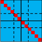
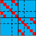
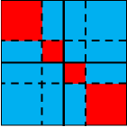
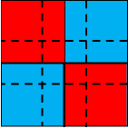
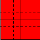
(a)	(b)	(c)	(d)	(e)

Figure 1: Adapted from Wahl (2018). Covariance matrices for different correlation assumptions. Rows and columns of the matrices correspond to the individual pencil beams, beam and ray separators indicate sections of pencil beams with the same irradiation angle and lateral position, respectively. (a) No correlation between pencil beams, (b) correlation of energy levels within one beam, (c) ray-wise correlation, all pencil beams with the same lateral position, i.e. hitting the same material are fully correlated (d) beam-wise correlation, pencil beams with the same irradiation angle are fully correlated and (e) errors in all pencil beams are fully correlated.

In case the correlation matrix is singular (perfect correlation between some pencil beams), the dimension of the uncertain vector can be reduced and one joint error can be sampled for the respective perfectly correlated pencil beams.

More complex correlation models are possible.

2.9 Implementation

For the proof-of-concept in this work, the weighting method was implemented as a post-processing routine in Matlab. Radiation plans were generated with matRad (Wieser et al.; 2017) and exported to the Monte Carlo simulation engine TOPAS (Perl et al.; 2012) for dose calculations. The required particle histories $h(\boldsymbol{\xi})$ are stored during the simulation using a custom extension for TOPAS.

All reference computations rely on Monte Carlo dose calculations with TOPAS as well.

To reduce the number of required realizations, both for the reference computation and the (re-)weighting steps, a quasi-Monte Carlo approach was used to sample the random parameters (see e.g. Caflisch; 1998).

2.10 Investigated patients and uncertainties

In the following, we consider range and set-up uncertainties, as well as a combination of both. For the set-up uncertainties, we assume a symmetric, bivariate normal distribution with zero mean (no systematic errors) and a standard deviation of $3\text{\,}\mathrm{mm}$ (comp. Wahl; 2018; Perkó et al.; 2016). For range uncertainties, in the reference computations we scale the density with a normally distributed factor, where the mean is equal to the nominal density and the standard deviation is $3\text{\,}\mathrm{\char 37\relax}$ (as recommended in Lomax; 2008b; Yang et al.; 2012). The corresponding parameters of the energy distribution, used to approximate range errors in the importance (re-)weighting estimate, are determined based on this distribution as detailed in 2.7. Table 1 provides an overview of which uncertainty models were computed for which patient, as well as the irradiation angles used for different patients.

Table 1: Overview of uncertainties investigated for each patient/test case. Beam irradiation angles are given as (couch angle, gantry angle) in degrees and error values refer to the standard deviations of the corresponding normal distributions.

		Patient	Water phantom	Prostate	Liver
		Angles	($0\mathrm{°}$, $0\mathrm{°}$)	($0\mathrm{°}$, $90\mathrm{°}$/$270\mathrm{°}$)	($0\mathrm{°}$, $315\mathrm{°}$)
Correlation	Type
Full	Set-up		$3\text{\,}\mathrm{mm}$	$3\text{\,}\mathrm{mm}$	$3\text{\,}\mathrm{mm}$
	Range		$3\text{\,}\mathrm{\char 37\relax}$	-	$3\text{\,}\mathrm{\char 37\relax}$
	Both		$3\text{\,}\mathrm{mm}$/$3\text{\,}\mathrm{\char 37\relax}$	-	$3\text{\,}\mathrm{mm}$/$3\text{\,}\mathrm{\char 37\relax}$
Beam	Set-up		-	$3\text{\,}\mathrm{mm}$	-
Ray	Set-up		-	$3\text{\,}\mathrm{mm}$	-
Energy	Both		-	$3\text{\,}\mathrm{mm}$/$3\text{\,}\mathrm{\char 37\relax}$	-
None	Set-up		-	$3\text{\,}\mathrm{mm}$	-

The number of histories and pencil beams for each considered patient, as well as the number of error scenarios computed for the importance (re-)weighting estimates can be found in table 2. Note, that the number of histories per pencil beam were determined based on (non-normalized) weights from the optimized radiation plan (see 2.9), where around $10^{5}$ histories are computed for the pencil beams with the highest weights.

Table 2: Overview of simulated plans and error scenarios per patient.

Patient	Water phantom	Liver	Prostate
Irradiation angles	00 ($0\mathrm{°}$, $0\mathrm{°}$)	0($0\mathrm{°}$, $315\mathrm{°}$)	00($0\mathrm{°}$, $90\mathrm{°}$)	0($0\mathrm{°}$, $270\mathrm{°}$)
Number of pencil beams	00000147	000001 378	000001 375	000001 383
Number of histories	2 566 453	13 528 430	16 992 193	16 748 034
Number of error scenarios	00000100	000000100	100

2.11 Evaluation criteria

To compare our results to the respective reference computations, we plot two-dimensional slices of the dose cubes as well as a difference map and employ a global three-dimensional $\gamma$-analysis. For the difference maps, we compute

$$\text{diff}_{i}(d^{\text{ref}}_{i},d_{i}^{\text{est}})=d_{i}^{\text{ref}}-d_{i}^{\text{est}}\;,$$ (20)

for each voxel $i$ in the reference result $d^{\text{ref}}$ and (re-)weighting estimate $d^{\text{est}}$. For the $\gamma$-analysis, we use the matRad implementation based on Low et al. (1998), with a distance to agreement of $3\text{\,}\mathrm{mm}$ and a dose difference criterion of $3\text{\,}\mathrm{\char 37\relax}$.

3 Results

In the following we present results for the cases given in table 1. Unless specified otherwise, results were computed on the basis of histories from nominal dose calculations, i.e. with phase space parameters sampled from $\Phi_{0}$ (see 2.2). The references computed for nominal and expected dose stem from Monte Carlo dose calculations with the respective phase space distributions $\Phi_{0}$ and $\Psi$ (see 2.4), the reference standard deviation is derived using numerous such Monte Carlo simulations for different error scenarios sampled from the joint error distribution. Therefore, the importance (re-)weighting estimate for the nominal dose only differs from the reference by round-off errors introduced in post-processing, as can be seen in figure 2. It is omitted thereafter, as is the reference.

3.1 Set-up errors

Figure 2 displays the nominal dose, expected value and standard deviation estimates for a water phantom, computed using the (re-)weighting approach in comparison to the respective references. While we see some minor deviations in difference maps for the expected dose and standard deviations, they do not appear systematic.

The distance-to-agreement analysis using the $\gamma$-criterion supports this quantitatively (table 3), with $\gamma^{$3\text{\,}\mathrm{mm}$}_{$3\text{\,}\mathrm{\char 37\relax}$}$-pass rate of $100\text{\,}\mathrm{\char 37\relax}$ for the nominal and expected dose and $99.97\text{\,}\mathrm{\char 37\relax}$ for the standard deviation. Figure 3 demonstrates that this is transferable to the more complex patient cases. With overall $\gamma^{$3\text{\,}\mathrm{mm}$}_{$3\text{\,}\mathrm{\char 37\relax}$}$-pass rates of $99.99\text{\,}\mathrm{\char 37\relax}$ (prostate patient) and $100\text{\,}\mathrm{\char 37\relax}$ (liver patient), the standard deviation agrees as well with the reference computations as the expected value, with $100\text{\,}\mathrm{\char 37\relax}$ and $99.99\text{\,}\mathrm{\char 37\relax}$, respectively (table 4, 5).

Table 3: $\gamma^{$3\text{\,}\mathrm{mm}$}_{$3\text{\,}\mathrm{\char 37\relax}$}$-pass rates in volumes of interest (VOI) of the water phantom.

Water Phantom	Nominal dose	Expected value	Standard deviation
Error type	Set-up
Overall	100	100	099.97
Body	100	100	099.97
Target	100	100	100

	Estimate	Reference	Difference
$\boldsymbol{d}$
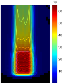
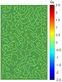
$E[\boldsymbol{d}]$
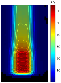
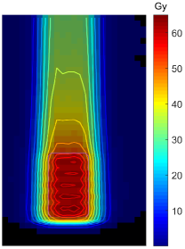
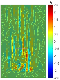
$\boldsymbol{\sigma(d)}$

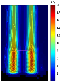
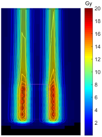
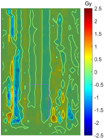
Figure 2: Nominal dose $\boldsymbol{d}$, expected dose $E[\boldsymbol{d}]$ and standard deviation $\boldsymbol{\sigma(d)}$ w.r.t. set-up uncertainties with $3\text{\,}\mathrm{mm}$ standard deviation for a spread out Bragg peak in a water phantom. The left column shows the estimate computed with the proposed (re-)weighting approach, the middle column the respective reference and the right column the difference between both simulations.

	Estimate	Difference	Estimate	Difference
$E[\boldsymbol{d}]$
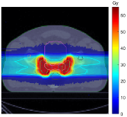
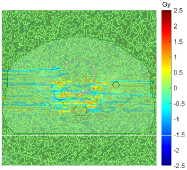
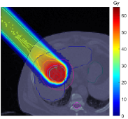
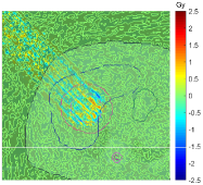
$\boldsymbol{\sigma(d)}$
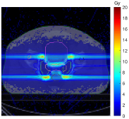
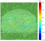
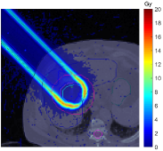
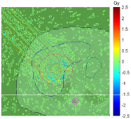
	(a) Prostate		(b) Liver

Figure 3: Expected dose $E[\boldsymbol{d}]$ and standard deviation $\boldsymbol{\sigma(d)}$ w.r.t. set-up uncertainties with $3\text{\,}\mathrm{mm}$ standard deviation for (a) a prostate patient (couch angle $0\mathrm{°}$, gantry angles $90\mathrm{°}$ and $270\mathrm{°}$) and (b) a liver patient (couch angle $0\mathrm{°}$, gantry angle $315\mathrm{°}$). The left columns show the estimates computed with the proposed (re-)weighting approach and the right columns the difference to the corresponding references.

Table 4: $\gamma^{$3\text{\,}\mathrm{mm}$}_{$3\text{\,}\mathrm{\char 37\relax}$}$-pass rates in volumes of interest (VOI) of the prostate patient.

Prostate	Expected value	Standard deviation
Error type	Set-up
Overall	100	099.99
Rectum	100	100
Penile bulb	100	100
Lymph nodes	100	100
Rt femoral head	100	100
Prostate bed	100	100
PTV 68	100	100
PTV 56	100	099.99
Bladder	100	099.99
Body	100	099.99
Lt femoral head	100	100

Table 5: $\gamma^{$3\text{\,}\mathrm{mm}$}_{$3\text{\,}\mathrm{\char 37\relax}$}$-pass rates in volumes of interest (VOI) of the liver patient (initial particles sampled from $\Phi_{0}$).

Liver	Expected Value			Standard Deviation
Error type	Set-up	Range	both	Set-up	Range	both
Overall	099.99	100	99.50	100	91.69	93.12
GTV	100	100	97.59	100	99.01	87.10
Liver	100	100	99.75	099.99	92.78	84.04
Heart	100	100	96.67	100	91.26	98.84
CTV	100	100	98.90	100	93.01	90.99
Contour	100	100	98.69	100	91.48	90.75
PTV	100	100	99.28	099.99	83.60	90.69

3.2 Range errors

In contrast to the set-up errors, for which dose estimates can also be shown to be mathematically accurate, range errors can only be modeled through an approximation introduced in 2.7. Figure 4 displays results for range errors as well as the combination of range and set-up errors in the water phantom.

The difference maps for both expected value and standard deviation show that the deviations when including range errors are expectedly higher. We observe a systematic bias primarily at the distal edge, where our method seems to consistently underestimate the variance. The standard deviation estimate using our importance weighting method also expresses strong local artifacts, as evident in the difference maps (compare figure 4). This is an indicator of too little statistical mass, i.e., computed particle trajectories, in the original simulation. For more extreme error realizations, relatively high weights are assigned to a small number of particles, thereby amplifying single realizations or errors. Especially in case of a relatively small beam energy spread in the original simulation (here $1\text{\,}\mathrm{\char 37\relax}$), compared to the range error of $3\text{\,}\mathrm{\char 37\relax}$, such artifacts are likely to appear. In order to prevent this, one could either compute a larger number of particle histories in the simulation or sample the particles from a different distribution which has more density mass in its outer regions or tails (compare 2.4).

To underline the explanation for the appearance of the artifacts above, we recomputed the estimates using the (re-)weighting method based on a direct computation of the expected value, which can be calculated using the convolution $\Psi$ of the Gaussian error kernel with the nominal phase space parameter distribution 2.4. Figure 4 shows that this alleviates the discrepancy from the references, causing artifacts to disappear and also reducing the overall amount of deviation displayed in the difference maps.

	Estimate ($\Phi_{0}$)	Difference	Estimate ($\Psi$)	Difference
$E[\boldsymbol{d}]$
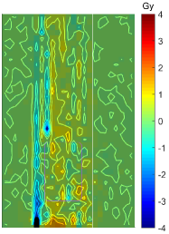
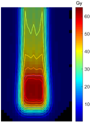
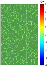
$\boldsymbol{\sigma(d)}$
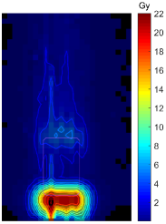
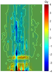
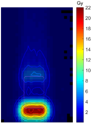
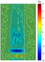
	(a) Range errors
	Estimate ($\Phi_{0}$)	Difference	Estimate ($\Psi$)	Difference
$E[\boldsymbol{d}]$
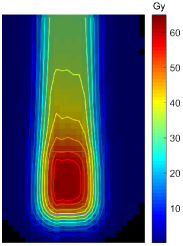
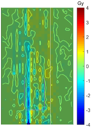
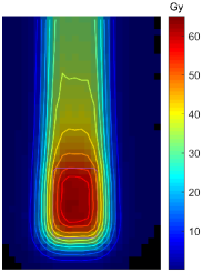
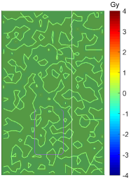
$\boldsymbol{\sigma(d)}$
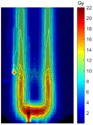
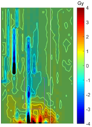
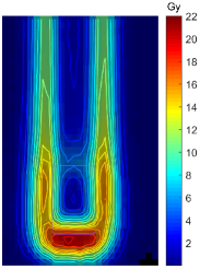
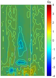
	(b) Range and set-up errors

Figure 4: Expected dose $E[\boldsymbol{d}]$ and standard deviation $\boldsymbol{\sigma(d)}$ w.r.t. (a) range uncertainties with a $3\text{\,}\mathrm{\char 37\relax}$ standard error (b) and both range uncertainties as well as set-up errors with $3\text{\,}\mathrm{mm}$ standard deviation for a spread out Bragg peak in a water phantom. The left columns show the estimate computed with the proposed (re-)weighting approach, reconstructed either from the nominal distribution $\Phi_{0}$ or its convolution $\Psi$ witht the error kernel. The right columns show the difference to the corresponding references.

	Estimate ($\Phi_{0}$)	Difference	Estimate ($\Psi$)	Difference
$E[\boldsymbol{d}]$
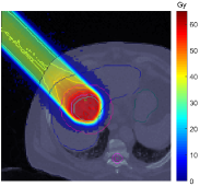
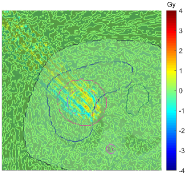
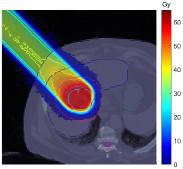
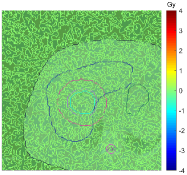
$\boldsymbol{\sigma(d)}$
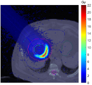
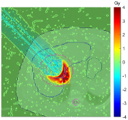
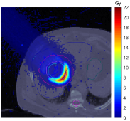
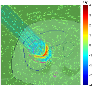
	(a) Range errors
	Estimate ($\Phi_{0}$)	Difference	Estimate ($\Psi$)	Difference
$E[\boldsymbol{d}]$
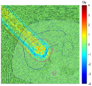
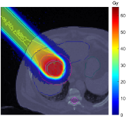
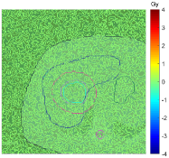
$\boldsymbol{\sigma(d)}$
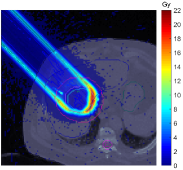
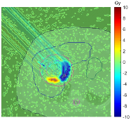
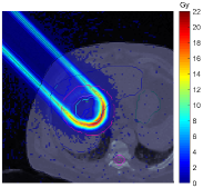
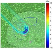
	(b) Range and set-up errors

Figure 5: Expected dose $E[\boldsymbol{d}]$ and standard deviation $\boldsymbol{\sigma(d)}$ w.r.t. (a) range uncertainties with a $3\text{\,}\mathrm{\char 37\relax}$ standard error and (b) both range uncertainties as well as set-up errors with $3\text{\,}\mathrm{mm}$ standard deviation in a liver patient (couch angle $0\mathrm{°}$, gantry angle $315\mathrm{°}$). The left columns show the estimate computed with the proposed (re-)weighting approach, reconstructed either from the nominal distribution $\Phi_{0}$ or its convolution $\Psi$ with the error kernel. The right columns show the difference to the corresponding references.

Thereby we can conclude that the irregularities in the solution can be attributed to the lack of statistical support in certain areas. Contrary to this, parts of the systematic differences remain and are thus most likely a result of the model approximations.

Figure 5 validates these observations for a liver patient. The difference maps for estimates computed based on the expected distribution $\Psi$, have less severe artifacts and systematic deviations. For both set-up and range errors, the $\gamma_{$3\text{\,}\mathrm{\char 37\relax}$}^{$3\text{\,}\mathrm{mm}$}$-pass rate also increases from $93.12\text{\,}\mathrm{\char 37\relax}$ to $98.19\text{\,}\mathrm{\char 37\relax}$ (table 5). However, we do not observe such an increase in the case of only range uncertainties.

Also, it has to be noted, that using $\Psi$ to sample the initial particles leads to an expected dose estimate which is exact up to machine precision, but a nominal dose estimate which now shows deviations from a nominal standard Monte Carlo reference computation in the order of magnitude that we could previously observe for the expected dose.

3.3 Correlation models

So far, we have only shown results for the case of fully correlated pencil beams, meaning one global shift of the patient position or scaling factor for the beam range. One of the advantages of the proposed method is, however, the high flexibility in changing the uncertainty model. In figure 6 we therefore present the standard deviation estimate for four examples of different error correlation models discussed in section 2.8.

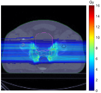
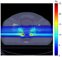
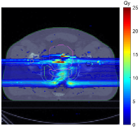
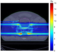
(a)	(b)	(c)	(d)

Figure 6: Standard deviation of dose in a prostate patient for (a) no correlation (b) correlation between pencil beams in the same energy level (c) ray-wise correlation between pencil beams and (d) correlation between pencil beams with the same irradiation angle, w.r.t set-up errors and in case (c) also range errors.

The results indicate, that different correlation assumptions have a crucial impact on the standard deviation of dose distributions. While it is in principle possible to define arbitrary correlations within the proposed framework, estimates can be prone to artifacts due to a lack of statistical information, especially for the ray-wise correlation model. When sampling error realizations independently for smaller beam components, the reconstruction depends solely on the particle histories associated with these components. For rays with small weights, only very few histories are computed, therefore we observe similar artifacts as encountered in above range uncertainty computations (3.2).

4 Accuracy and Convergence

Mathematically, it can be shown, that the expected and nominal dose estimates are unbiased. This also holds for the doses corresponding to each individual error realization. While this does not generally apply for the variance, our results indicate that the bias does not have a significant impact on the quality of estimates.

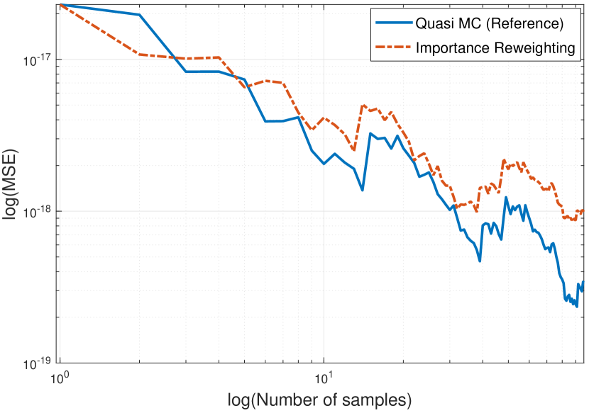
(a)

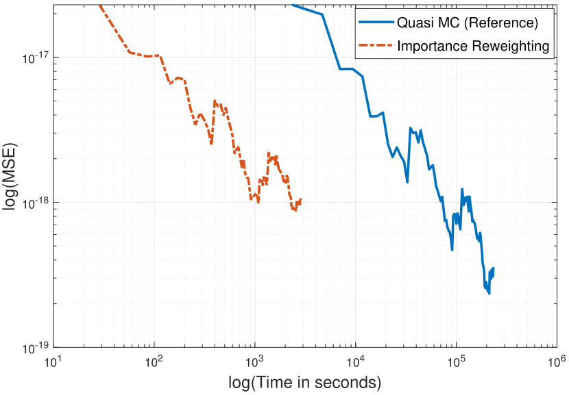
(b)

Figure 7: Mean square error (MSE) of the dose standard deviation estimate for the water phantom, computed using a (quasi) Monte Carlo method and the importance (re-)weighting approach and compared for the error convergence (a) per number of samples and (b) per corresponding computation time.

For quicker convergence we used quasi-random numbers throughout the whole comparisons, both for the reference computation and the importance (re-)weighting approach. Note, that the combination of importance sampling with quasi-Monte Carlo methods has been shown to be not only possible, but advantageous and preserves the convergence properties of quasi-Monte Carlo (Hörmann and Leydold; 2005; Ökten; 1999; Caflisch; 1998; Schürer; 2004). Since the procedure mimics a (quasi-) Monte Carlo method for uncertainty quantification, where the repeated simulation runs are replaced by (re-)weighting steps, the convergence of the variance per computed error realization is identical. However, due to the lower cost of the (re-)weighting steps, the convergence per time is much faster (see figure 7).

Table 6: CPU time comparison for the reference vs. (re-)weighting approach applied to different patients and computed on the same machine. All values are given in seconds. Note that the times for 100 realizations include the initialization times, while the time for a single realization only refers to the dose computation time.

		Reference	(Re-)weighting
Water phantom	Initialization	00000002.35	0000061.53
	One realization	0002 331.30	0000028.51
	100 realizations	0233 126.93	002 912.53
Liver	Initialization	00000002.44	002 038.75
	One realization	0039 066.44	001 198.74
	100 realizations	3 906 650.90	121 912.75
Prostate	Initialization	00000004.26	004 867.75
	One realization	0058 762.40	002 479.07
	100 realizations	5 876 253.86	252 774.75

For run-time comparisons, the reference computations using TOPAS and the (re-)weighting approach, implemented as post-processing in Matlab, were run on the same virtual machine. We observe reduced CPU times by a factor of 80, 32 and 23 for the water phantom, liver and prostate patient, respectively (see table 6).

5 Discussion

In this paper, we introduce an efficient approach for uncertainty quantification in Monte Carlo dose calculations using history (re-)weighting. We demonstrate how particle histories from one simulation can be scored to construct estimates for error scenarios, the expected dose and standard deviation, for set-up and range errors in intensity modulated proton therapy. As demonstration example, Gaussian range and set-up uncertainties, with $3\text{\,}\mathrm{\char 37\relax}$ and $3\text{\,}\mathrm{mm}$ standard deviation respectively, were considered for a water phantom, a liver patient and a prostate patient.

For set-up uncertainties, we observed good agreement of at least $99.99\text{\,}\mathrm{\char 37\relax}$ in the $\gamma_{$3\text{\,}\mathrm{mm}$/$3\text{\,}\mathrm{\char 37\relax}$}$-criterion for all quantities of interest. Range error propagation could be approximated by transforming the assumed range uncertainty into energy uncertainty via the range-energy relationship. The error caused by this model approximation appears to be relatively minor for the expected dose. The standard deviation estimates are, however, sensitive to the number of histories and usage of the nominal Gaussian pencil beam width or the convolved distribution. Differences and visible artifacts in the standard deviation estimate can be partly eliminated by simulating the initial phase-space parameters using the convolved beam parameterization. While some systematic deviations remain, the order of magnitude as well as shape and extent of the dose standard deviation is sufficiently well-represented. However, this causes a reduction in accuracy for the nominal dose. Thus, improving the accuracy of the estimate for one quantity of interest comes at a cost for the accuracy of another and it remains up to the user and use-case to put the focus on either retaining accuracy in the nominal dose computation or trading it against better accuracy of the uncertainty estimate.

We also demonstrate the use of different pencil beam correlation models within the framework. It is clear that the choice of correlation model has a significant impact on the standard deviation estimate. Therefore, it is particularly convenient that the (re-)weighting method allows for the definition of principally arbitrary correlation matrices to put into the underlying multivariate Gaussian error model. These could possibly be extended to simulate interplay effects or other dynamic influences in the context of 4D treatment planning. Since the applied correlation models are not only experimental but also difficult and time-consuming to evaluate in scenario sampling, we did not quantitatively compare them to reference computations. Further studies could explore whether they agree with other methods computing such correlations based on an analytical probabilistic dose engine (Bangert et al.; 2013; Wahl et al.; 2017; Wieser et al.; 2020).

Compared to the reference scenario estimates, which rely on performing full MC dose calculations repeatedly, the CPU-time for standard deviation estimates could be reduced by more than an order of magnitude using our method in combination with a quasi-MC approach. This is achieved by reducing the costs of repeated expensive simulations to those of scoring based on matrix-vector multiplications. Consequently, it has to be noted, that the time reduction depends largely on the proportion of computational overhead of the initialization and simulation steps in the MC engine. Therefore the factor of speed increase varies strongly between different test-cases and, most likely, implementations. But even then, our method holds two performance advantages: First, it can directly compute the expected dose by using the convolved phase space parameterization (2.4) in one standard simulation. Second, multiple uncertainty models with different correlation patterns and magnitude can be reconstructed from the same set of histories. This could for example be used to investigate the impact of fractionation effects, using the framework proposed by Wahl et al. (2018) or to consider a number of (worst case) scenarios besides the expected dose and standard deviation.

Further, we argue that computational performance can be further improved through a more efficient implementation and using better parallelization. Also, a combination of our approach with other efficient uncertainty quantification approaches, which rely on scenario computations could lead to run-time improvements. For instance a polynomial chaos expansion as introduced in Perkó et al. (2016) could be adjusted such that the evaluations are computed by (re-)weighting histories instead of the usual dose calculations.

When computing the estimates in post-processing, the regular Monte Carlo dose calculation is not slowed down perceptibly by storing particle histories for later reconstructions. The possible additional run-time is smaller than the variation between two runs of the same simulation and thereby barely detectable. An implementation as on-the-fly scoring is however also possible and might outperform post-processing in terms of overall run time for a single uncertainty model.

Last but not least, the method is not inherently limited to the discussed application in proton therapy; a calculation of uncertainty estimates using the (re-)weighting approach would also be feasible for other IMPT modalities like carbon ions but also photons. In its current description, it is however limited to uncertainties which can be modeled in terms of variations of phase space parameters with a prior probability distribution. Application to, for example, pre-simulated phase spaces might also be feasible using numerical convolution techniques. Also, a disproportionately high magnitude of uncertainties in relation to this probability distribution can compromise the accuracy of results. Furthermore, it needs to be mentioned, that the current computational speed, especially for the standard deviation, might still not be sufficient for optimization purposes, where a full dose influence matrix needs to be computed. Due to the simplicity of the process and the high flexibility in post-processing at virtually no cost for the original simulation, we are confident that the approach has the potential for further development and use.

6 Conclusion

Dose distributions in intensity modulated proton therapy are known to be sensitive to uncertainties. The computational efforts in estimating such uncertainties become particularly evident when Monte Carlo dose calculation is used. We showed how the concept of importance sampling can be adapted to estimate the expected dose and its variance using histories from only a single Monte Carlo simulation. Set-up uncertainties can be efficiently modeled and exhibit almost exact agreement with reference computations. The inclusion of range uncertainties, by modeling them as energy uncertainty via the range-energy relationship, yields less but sufficient accuracy for most application purposes. Further, the physical simulation of particles is completely decoupled from uncertainty quantification, thereby allowing for the incorporation of arbitrary correlation assumptions and the comparison of different scenarios, at no additional cost to the nominal dose calculation. Therefore, the presented approach has several benefits over classic non-intrusive methods and is a step towards reconciling efficient uncertainty quantification and, in the future, robust optimization based on Monte Carlo dose calculations.

Appendix A Importance Sampling

Importance sampling is a method most frequently used for variance reduction (Kahn; 1950; Hastings; 1970). Assume the integral $I(g)=\int g(x)p(x)dx$ is to be computed for $x\sim p(x)$ without directly sampling from $p(x)$. The importance sampling estimate is defined as

$$I(g) =\int g(x)p(x)dx=\int g(x)\frac{p(x)}{q(x)}q(x)dx$$ (21)

$$\approx\sum_{i=1}^{N}g(X_{i})\frac{p(X_{i})}{q(X_{i})}\;,\;\;X_{i}\sim q(x)$$

Thus, the integral of $g(x)$ with the probability distribution $x\sim p(x)$ can be reconstructed from samples of a suitable density function $q(x)$.

Appendix B Full phase space model

The simplified model used in the main paper can be extended to include distributions in the momentum direction $\boldsymbol{\varphi}=(\varphi_{x},\varphi_{y},\varphi_{z})\neq 0$. The additional variables are included in the Gaussian mixture model:

$$\Phi_{0}(\boldsymbol{\xi})=\sum_{b=1}^{B}w_{b}\Phi_{0}^{b}(\boldsymbol{\xi})\;,\Phi_{0}^{b}(\boldsymbol{\xi})=\Phi_{0}^{b}(\boldsymbol{r},\boldsymbol{\varphi},E)=\mathcal{N}(\boldsymbol{\mu}_{\xi}^{b},\boldsymbol{\Sigma}_{\xi}^{b})$$ (22)

where the respective entries in the covariance matrix $\Sigma_{\xi}^{b}$ can be chosen $\neq 0$ to model randomness in the momentum direction as well as correlations of the momentum directions with primary particle positions.

Table 7: $\gamma^{$3\text{\,}\mathrm{mm}$}_{$3\text{\,}\mathrm{\char 37\relax}$}$-pass rates in volumes of interest (VOI) of the liver patient computed using the full phase space parameterizations.

	From $\Phi_{0}$			From $\Psi$
Error type	Set-up
Liver	$\boldsymbol{d}$	$E[\boldsymbol{d}]$	$\boldsymbol{\sigma(d)}$	$\boldsymbol{d}$	$E[\boldsymbol{d}]$	$\boldsymbol{\sigma(d)}$
Overall	100	099.99	099.77	099.99	100	099.74
GTV	100	100	100	100	100	100
Liver	100	100	099.78	100	100	099.79
Heart	100	100	099.83	100	100	099.53
CTV	100	100	099.64	100	100	099.51
Contour	100	100	099.81	100	100	099.70
PTV	100	100	099.54	100	100	098.72

$\boldsymbol{d}$

Estimate ($\Phi_{0}$)

Estimate ($\Psi$)

Reference

$E[\boldsymbol{d}]$

$\boldsymbol{\sigma}$

Figure 8: Nominal dose, expected dose and standard deviation w.r.t. set-up uncertainties with $3\text{\,}\mathrm{mm}$ standard deviation for one beam (couch angle $0\mathrm{°}$, gantry angle $315\mathrm{°}$), computed using the full phase space parameterizations.

Figure 8 presents results for the nominal dose, expected dose and standard deviation in a liver patient, for set-up uncertainties with $3\text{\,}\mathrm{mm}$ standard deviation, $0.2$ standard deviation in the momentum direction and $0.3$ correlation between $\varphi_{v}$ and $r_{v},\;v\in\{x,y\}$. Estimates were computed based on the convolution function $\Psi$ of the error and beam parameter densities, as well as the nominal parameter density $\Phi_{0}$. The corresponding global $\gamma$-analysis pass rates can be found in table 7.

References

- (1)
- Bangert et al. (2013) Bangert, M., Hennig, P. and Oelfke, U. (2013). Analytical probabilistic modeling for radiation therapy treatment planning, Physics in Medicine and Biology 58(16): 5401–5419.
- Bielajew (1994) Bielajew, A. F. (1994). Monte Carlo modeling in external electron-beam radiotherapy—why leave it to chance, Proc. 11th ICCR (Manchester, UK) pp. 2–5.
- Bortfeld (1997) Bortfeld, T. (1997). An analytical approximation of the Bragg curve for therapeutic proton beams, Medical Physics 24(12): 2024–2033.
- Caflisch (1998) Caflisch, R. E. (1998). Monte Carlo and quasi-Monte Carlo methods, Acta Numerica 7: 1–49.
- Casiraghi et al. (2013) Casiraghi, M., Albertini, F. and Lomax, A. (2013). Advantages and limitations of the ’worst case scenario’ approach in IMPT treatment planning, Physics in medicine and biology 58: 1323–1339.
- Fippel and Soukup (2004) Fippel, M. and Soukup, M. (2004). A Monte Carlo dose calculation algorithm for proton therapy, Medical Physics 31(8): 2263–2273.
- Fredriksson (2012) Fredriksson, A. (2012). A characterization of robust radiation therapy treatment planning methods-from expected value to worst case optimization, Medical Physics 39(8): 5169–5181.
- Fredriksson et al. (2011) Fredriksson, A., Forsgren, A. and Hårdemark, B. (2011). Minimax optimization for handling range and setup uncertainties in proton therapy, Medical Physics 38(3): 1672–1684.
- Hastings (1970) Hastings, W. K. (1970). Monte Carlo Sampling Methods Using Markov Chains and Their Applications, Biometrika 57(1): 97–109.
- Hörmann and Leydold (2005) Hörmann, W. and Leydold, J. (2005). Quasi Importance Sampling.
- Hu and Jin (2016) Hu, J. and Jin, S. (2016). A stochastic Galerkin method for the Boltzmann equation with uncertainty, Journal of Computational Physics 315: 150–168.
- Kahn (1950) Kahn, H. (1950). Random sampling (Monte Carlo) techniques in neutron attenuation problems–I, Nucleonics 6(5): 27; passim.
- Kimstrand et al. (2007) Kimstrand, P., Traneus, E., Ahnesjö, A., Grusell, E., Glimelius, B. and Tilly, N. (2007). A beam source model for scanned proton beams, Physics in Medicine and Biology 52(11): 3151–3168.
- Kraan et al. (2013) Kraan, A. C., van de Water, S., Teguh, D. N., Al-Mamgani, A., Madden, T., Kooy, H. M., Heijmen, B. J. M. and Hoogeman, M. S. (2013). Dose uncertainties in IMPT for oropharyngeal cancer in the presence of anatomical, range, and setup errors, International Journal of Radiation Oncology, Biology, Physics 87(5): 888–896.
- Liu et al. (2012) Liu, W., Zhang, X., Li, Y. and Mohan, R. (2012). Robust optimization of intensity modulated proton therapy, Medical Physics 39(2): 1079–1091.
- Lomax (2008a) Lomax, A. J. (2008a). Intensity modulated proton therapy and its sensitivity to treatment uncertainties 1: The potential effects of calculational uncertainties., Physics in medicine and biology 53(4): 1027–1042.
- Lomax (2008b) Lomax, A. J. (2008b). Intensity modulated proton therapy and its sensitivity to treatment uncertainties 2: The potential effects of inter-fraction and inter-field motions., Physics in medicine and biology 53(4): 1043–1056.
- Low et al. (1998) Low, D. A., Harms, W. B., Mutic, S. and Purdy, J. A. (1998). A technique for the quantitative evaluation of dose distributions, Medical Physics 25(5): 656–661.
- Lowe et al. (2016) Lowe, M., Albertini, F., Aitkenhead, A., Lomax, A. J. and MacKay, R. I. (2016). Incorporating the effect of fractionation in the evaluation of proton plan robustness to setup errors, Physics in Medicine and Biology 61(1): 413–429.
- Ma et al. (2002) Ma, C.-M., Li, J. S., Pawlicki, T., Jiang, S. B., Deng, J., Lee, M. C., Koumrian, T., Luxton, M. and Brain, S. (2002). A Monte Carlo dose calculation tool for radiotherapy treatment planning, Physics in Medicine and Biology 47(10): 1671–1689.
- Mackie (1990) Mackie, T. (1990). Applications of Monte Carlo method in radiotherapy, Dosimetry of Ionizing Radiation pp. 541–620.
- Malyapa et al. (2016) Malyapa, R., Lowe, M., Bolsi, A., Lomax, A. J., Weber, D. C. and Albertini, F. (2016). Evaluation of Robustness to Setup and Range Uncertainties for Head and Neck Patients Treated With Pencil Beam Scanning Proton Therapy, International Journal of Radiation Oncology*Biology*Physics 95(1): 154–162.
- McGowan et al. (2015) McGowan, S. E., Albertini, F., Thomas, S. J. and Lomax, A. J. (2015). Defining robustness protocols: A method to include and evaluate robustness in clinical plans, Physics in Medicine and Biology 60(7): 2671–2684.
- McGowan et al. (2013) McGowan, S. E., Burnet, N. G. and Lomax, A. J. (2013). Treatment planning optimisation in proton therapy, The British Journal of Radiology 86(1021): 20120288–20120288.
- Ökten (1999) Ökten, G. (1999). Error reduction techniques in quasi-monte carlo integration, Mathematical and Computer Modelling 30(7): 61–69.
- Paganetti (2012) Paganetti, H. (2012). Range uncertainties in proton therapy and the role of Monte Carlo simulations, Physics in Medicine and Biology 57(11): R99–R117.
- Park et al. (2013) Park, P. C., Cheung, J. P., Zhu, X. R., Lee, A. K., Sahoo, N., Tucker, S. L., Liu, W., Li, H., Mohan, R., Court, L. E. and Dong, L. (2013). Statistical assessment of proton treatment plans under setup and range uncertainties., International journal of radiation oncology, biology, physics 86(5): 1007–1013.
- Pedroni et al. (2005) Pedroni, E., Scheib, S., Böhringer, T., Coray, A., Grossmann, M., Lin, S. and Lomax, A. (2005). Experimental characterization and physical modelling of the dose distribution of scanned proton pencil beams, Physics in Medicine and Biology 50(3): 541–561.
- Perkó et al. (2016) Perkó, Z., van der Voort, S. R., van de Water, S., Hartman, C. M. H., Hoogeman, M. and Lathouwers, D. (2016). Fast and accurate sensitivity analysis of IMPT treatment plans using Polynomial Chaos Expansion, Physics in Medicine and Biology 61(12): 4646–4664.
- Perl et al. (2012) Perl, J., Shin, J., Schumann, J., Faddegon, B. and Paganetti, H. (2012). TOPAS: An innovative proton Monte Carlo platform for research and clinical applications, Medical Physics 39(11): 6818–6837.
- Pflugfelder et al. (2008) Pflugfelder, D., Wilkens, J. J. and Oelfke, U. (2008). Worst case optimization: A method to account for uncertainties in the optimization of intensity modulated proton therapy., Physics in medicine and biology 53(6): 1689–1700.
- Poëtte (2018) Poëtte, G. (2018). A gPC-intrusive Monte-Carlo scheme for the resolution of the uncertain linear Boltzmann equation, Journal of Computational Physics .
- Schürer (2004) Schürer, R. (2004). Adaptive Quasi-Monte Carlo Integration Based on MISER and VEGAS, in H. Niederreiter (ed.), Monte Carlo and Quasi-Monte Carlo Methods 2002, Springer, Berlin, Heidelberg, pp. 393–406.
- Sobotta et al. (2010) Sobotta, B., Söhn, M. and Alber, M. (2010). Robust optimization based upon statistical theory, Medical Physics 37(8): 4019–4028.
- Soukup et al. (2005) Soukup, M., Fippel, M. and Alber, M. (2005). A pencil beam algorithm for intensity modulated proton therapy derived from Monte Carlo simulations, Physics in Medicine and Biology 50(21): 5089–5104.
- Souris et al. (2019) Souris, K., Montero, A. B., Janssens, G., Perri, D. D., Sterpin, E. and Lee, J. A. (2019). Technical Note: Monte Carlo methods to comprehensively evaluate the robustness of 4D treatments in proton therapy, Medical Physics 46(10): 4676–4684.
- Taylor et al. (2017) Taylor, P. A., Kry, S. F. and Followill, D. S. (2017). Pencil Beam Algorithms Are Unsuitable for Proton Dose Calculations in Lung, International Journal of Radiation Oncology*Biology*Physics 99(3): 750–756.
- Tourovsky et al. (2005) Tourovsky, A., Lomax, A. J., Schneider, U. and Pedroni, E. (2005). Monte Carlo dose calculations for spot scanned proton therapy, Physics in Medicine and Biology 50(5): 971–981.
- Ulmer and Matsinos (2011) Ulmer, W. and Matsinos, E. (2011). Theoretical methods for the calculation of Bragg curves and 3D distributions of proton beams, The European Physical Journal Special Topics 190: 1–81.
- Unkelbach et al. (2018) Unkelbach, J., Alber, M., Bangert, M., Bokrantz, R., Chan, T. C. Y., Deasy, J. O., Fredriksson, A., Gorissen, B. L., van Herk, M., Liu, W., Mahmoudzadeh, H., Nohadani, O., Siebers, J. V., Witte, M. and Xu, H. (2018). Robust radiotherapy planning, Physics in Medicine and Biology 63(22): 22TR02.
- Unkelbach et al. (2009) Unkelbach, J., Bortfeld, T., Martin, B. C. and Soukup, M. (2009). Reducing the sensitivity of IMPT treatment plans to setup errors and range uncertainties via probabilistic treatment planning, Medical Physics 36(1): 149–163.
- Unkelbach et al. (2007) Unkelbach, J., Chan, T. C. and Bortfeld, T. (2007). Accounting for range uncertainties in the optimization of intensity modulated proton therapy, Physics in Medicine & Biology 52(10): 2755.
- Wahl (2018) Wahl, N. (2018). Analytical Models for Probabilistic Inverse Treatment Planning in Intensity-Modulated Proton Therapy, PhD Thesis.
- Wahl et al. (2017) Wahl, N., Hennig, P., Wieser, H.-P. and Bangert, M. (2017). Efficiency of analytical and sampling-based uncertainty propagation in intensity-modulated proton therapy, Physics in Medicine and Biology 62(14): 5790–5807.
- Wahl et al. (2018) Wahl, N., Hennig, P., Wieser, H.-P. and Bangert, M. (2018). Analytical incorporation of fractionation effects in probabilistic treatment planning for intensity-modulated proton therapy, Medical Physics 45(4): 1317–1328.
- Wahl et al. (2020) Wahl, N., Hennig, P., Wieser, H.-P. and Bangert, M. (2020). Analytical probabilistic modeling of dose-volume histograms, Medical Physics 47(10): 5260–5273.
- Weng et al. (2003) Weng, X., Yan, Y., Shu, H., Wang, J., Jiang, S. and Luo, L. (2003). A vectorized Monte Carlo code for radiotherapy treatment planning dose calculation, Physics in medicine and biology 48: N111–20.
- Wieser et al. (2017) Wieser, H.-P., Cisternas, E., Wahl, N., Ulrich, S., Stadler, A., Mescher, H., Müller, L.-R., Klinge, T., Gabrys, H., Burigo, L., Mairani, A., Ecker, S., Ackermann, B., Ellerbrock, M., Parodi, K., Jäkel, O. and Bangert, M. (2017). Development of the open-source dose calculation and optimization toolkit matRad., Medical physics 44(6): 2556–2568.
- Wieser et al. (2020) Wieser, H.-P., Karger, C. P., Wahl, N. and Bangert, M. (2020). Impact of Gaussian uncertainty assumptions on probabilistic optimization in particle therapy, Physics in Medicine & Biology 65(14): 145007.
- Yang et al. (2012) Yang, M., Zhu, X. R., Park, P. C., Titt, U., Mohan, R., Virshup, G., Clayton, J. E. and Dong, L. (2012). Comprehensive analysis of proton range uncertainties related to patient stopping-power-ratio estimation using the stoichiometric calibration, Physics in Medicine and Biology 57(13): 4095–4115.