Parallel decomposition of persistence modules through interval bases

Abstract

We introduce an algorithm to decompose any finite-type persistence module with coefficients in a field into what we call an interval basis. This construction yields both the standard persistence pairs of Topological Data Analysis (TDA), as well as a special set of generators inducing the interval decomposition of the Structure theorem. The computation of this basis can be distributed over the steps in the persistence module. This construction works for general persistence modules on a field ${\mathbb{F}}$, not necessarily deriving from persistent homology. We subsequently provide a parallel algorithm to build a persistent homology module over ${\mathbb{R}}$ by leveraging the Hodge decomposition, thus providing new motivation to explore the interplay between TDA and the Hodge Laplacian.

Keywords— Graded module decomposition; persistent homology; Hodge decomposition; Hodge Laplacian
Mathematics Subject Classification (2020)— 13P20, 55N31, 62R40

1 Introduction

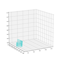
(a) Step 0

(b) Step 1

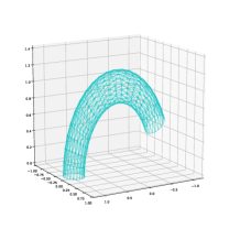
(c) Step 2

Figure 1: A 3-step filtration by sublevel sets, with respect to the the $z$ coordinate, of a half torus.

Consider a monotone persistence module $\mathcal{M}=\{M_{i},\varphi_{i}:M_{i}\to M_{i+1}\}_{i}$ over a field ${\mathbb{F}}$ (PM), indexed over the natural numbers where each $M_{i}$ is called $i^{th}$ step and each $\varphi_{i}$ is called $i^{th}$ structure map. Assume that the module is of finite type, i.e. that each ${\mathbb{F}}$-vector space $M_{i}$ is finite dimensional and only a finite number of maps among the $\varphi_{i}$’s are not isomorphisms.
This is the typical setting of persistent homology, the subject in which the name persistence module originally arose. The two fundamental properties of finite type persistent modules imply that each $\{M_{i},\varphi_{i}\}$ can be decomposed, up to ordering, into a direct sum of interval modules so that the module is completely described by its persistence diagram or barcode, and furthermore that this decomposition is stable with respect to noise if the PM is made of the homology groups of a geometric sampling.

These properties largely account for the success of Topological Data Analysis, a field that leverages computational techniques in algebraic topology to extract information from data.
More explicitly, a persistence module can be written uniquely, up to permutations of summands, as a direct sum of persistence (sub)modules

$$\mathcal{M}\cong\bigoplus_{m}I_{[b_{m},d_{m}]},$$ (1)

where each term $I_{[b_{m},d_{m}]}$, called interval, is an indecomposable persistence submodule depending on the indexes $b_{m}\leq d_{m}$. The multiset of pairs $\{(b_{m},d_{m})\}$ forms the barcode.
Under the isomorphism in Eq.(1), for each $m$, one might search for an element $v_{m}$ in $\mathcal{M}$ which, through the application of the structure maps, generates the submodule $I(v_{m})$ corresponding to $I_{[b_{m},d_{m}]}$.

In this work, we call a set of generators $\{v_{m}\}_{m}$ of $\mathcal{M}$ an interval basis if it satisfies

$$\mathcal{M}=\bigoplus_{m}I(v_{m})\cong\bigoplus_{m}I_{[b_{m},d_{m}]}.$$ (2)

The classical algorithm to construct the barcode of a finite type persistence module [5] works at the level of the chain complexes and thus is limited to persistence module induced by homology. The algorithm yields the pairs $\{(b_{m},d_{m})\}$, and can be used to extract a set of homology generators, as done in [13]. However, the extracted set of generators does not generally satisfy Eq. 2. For example, consider a filtration of the half torus such as the one depicted in Fig. 1, which will be our running example throughout the paper. The classical algorithm correctly identifies the persistence pairs, but returns the generators depicted in Fig. 2, in accordance with the so-called elder rule. These generators do not induce a decomposition such as the one in Eq. 2, because their images in the final step of the filtration become homologous. Algebrically, this entails a linear relation between non-zero elements of $\mathcal{M}$ and thus the sum of interval modules in Eq. 2 is not direct.
A principal contribution of this work is to provide a procedure to build an interval basis. From an interval basis, it is trivial to compute the persistence pairs. As an example, for the case of $1$-homology of the half torus, a set of generators forming an interval basis is depicted in Fig. 3.

With the classical approach one is only allowed to compute the decomposition of a persistence module that is the homology of a filtration of simplicial complexes. Moreover, the algorithm intrinsically works with objects (chain groups and chain maps) whose dimension is typically much larger than that of their homology module.
Our proposed method, instead, addresses the case of finding a decomposition of a general, i.e. not necessarily a homology, persistence module. As such, we work directly at the level of $\{M_{i},\varphi_{i}\}$. As a consequence, the bulk of our algorithm can be performed independently for each $M_{i}$, i.e. is largely parallelizable.

We can summarize the main contribution with the following result

Theorem.

Given a finite-type ${\mathbb{F}}$-persistence module, the output of Algorithm 3 provides an interval basis.

After giving a specific instance of our algorithm for the case of $k$-persistent homology modules, i.e., persistence modules obtained through the $k$-homology functor applied to a filtration, we specialize our procedure to the case where the chain spaces are Euclidean, i.e. have a scalar product. For example, we address the case of $k$-persistent homology modules with coefficients in ${\mathbb{R}}$, which can be built from the kernel of the $k$ Hodge Laplacian operator with respect to a filtration of simplicial complexes. We construct the induced maps between kernels and, by the known properties of the Hodge Laplacian, prove it to be equivalent to the $k$-persistent homology module. We then apply our decomposition to obtain an interval basis, which is shown in Fig. 4. This furthers the recent trend of exploring the interplay between topological data analysis and the properties of the Hodge Laplacian [10, 25, 26].

(a) Generator 1

(b) Generator 2

Figure 2: Generators, classical algorithm.

(a) Generator 1

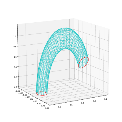
(b) Generator 2

Figure 3: Interval basis generators for the $k$-persistent homology module.

(a) Generator 1

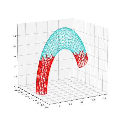
(b) Generator 2

Figure 4: Interval basis generators for the harmonic persistence module

Contributions and related work

The key results of this paper can be summarized as:

1. An algorithm for the decomposition of any monotone persistence module on any field. We do not assume the module is induced by homology. As such, the module might derive from any sequence of simplicial maps.

2. The generators we provide are such that a decomposition of the persistence module is given by the interval modules they each generate. We call this an interval basis.

3. Our algorithm is parallelizable for each step of the module.

We further provide a parallel algorithm to construct a persistence module from a general collection of simplicial maps. In the special case of real coefficients, we use the Hodge Laplacian as a construction method for homology groups and maps between them. We therefore specialize the decomposition algorithm.

The original approach to the decomposition of persistence modules arising from filtrations of simplicial complexes was introduced in [13], based on the simplex pairing approach of [7]. These algorithms were limited to working with ${\mathbb{Z}}_{2}$ coefficients and simplicial maps deriving from inclusions of simplicial complexes. Later, this framework was extended to arbitrary coefficient fields in [5], which established the notorious correspondence between persistence modules and graded modules over a PID. It is immediate to construct a set of generators from the output of these algorithms. However, they do not induce an interval basis decomposition of the module. A different approach to attempt a principled choice of homology generators is to introduce a notion of geometric minimality, as it was done in [9, 19, 16].
The distributed computation of the persistence pairs has been addressed in [1], where arguments from discrete Morse theory are employed to observe that the reduction of a boundary matrix obtained from a filtration of simplicial complexes can be performed in chunks. The chunk algorithm can, like the one proposed here, be run in parallel for each filtration step, and is incremental in that it only considers cells that are born within the step itself. Its objective, however, is to compute the persistence pairs of a filtration, whereas our proposal works for general (albeit monotone) simplicial maps, needs not consider the (typically much larger) space of $k$-chains and computes an interval basis.
Subsequently, the case of a monotone sequence of general simplicial maps was addressed in [8], which relies on the notion of simplex annotation. In this way, and by interpreting each simplicial map as a sequence of inclusions and vertex collapses, a consistent homology basis can be maintained efficiently. Later in [20] a variation of the coning approach of [8] is proposed, which takes a so-called simplicial tower and converts it into a filtration, while preserving its barcode, with asymptotically small overhead. Our approach to the problem is different in that we do not need to work at the level of simplicial complexes or maps, and in fact our decomposition is independent from the persistence module being induced by a filtration of simplicial complexes.
To our knowledge, the first paper to deal with persistence module decompositions without assuming it arises from a family of inclusion maps was an instance of topological persistence whose underlying structure is not monotone: the so-called zigzag persistence([4]). Zigzag persistence is based on a sequence of structure maps whose direction is not necessarily left to right. They provide an incremental algorithm which computes a decomposition of the zigzag module, without focusing on its generators. Our proposal differs in that we are restricted to the case of monotone persistence, but in turn our focus is on the construction of an interval basis, and on a parallel algorithm.
An analogous point of view is taken in a recent paper by Carlsson et al. ([3]). The decomposition of the general zigzag module is tackled from the matrix factorization viewpoint. Starting from a type-A quiver representation, their goal is to compute a basis for each homogenous component of a persistence module in such a way that the structure maps are represented as echelon form matrices. In other words, the matrix associated to the quiver representation is in canonical form. Our algorithm can decompose the module while avoiding the change of basis operations that are needed for the construction of the echelon form. Furthermore, by specializing to monotone persistence modules we can avoid the divide and conquer approach and instead perform computations in parallel across all degrees.

Structure of the paper

In the background Section 2 we review some concepts about persistence modules, not necessarily made by the homology of some space, and introduce our notion of interval basis in connection with the Structure Theorem. Section 3 introduces the main algorithm (Algorithm 3) to compute an interval basis of a general persistence module. In Section 4 we give a constructive method, acting independently over each step (Algorithm 6) and structure map (Algorithm 7), for constructing a $k$-persistent homology module. Moreover, we see how our constructive method can be adapted to the case of harmonic persistence module where each step is obtained as the kernel of the Hodge Laplacian operator, and each structure map is easily obtained via Algorithm 8. The Appendices contain bonus background material to support the proofs in Section 4 and to recall the construction from simplicial complexes to chain complexes in the usual TDA pipeline.

2 Background

In order to formalize the problem addressed in this work, we introduce the persistence module.

We define a persistence module $\mathcal{M}$ as pair $\{M_{i},\varphi_{i}\}_{i\in\mathbb{N}}$ consisting of, for any $i\in\mathbb{N}$:

• a finite-dimensional ${\mathbb{F}}$-vector space $M_{i}$ called step

• a linear map $\varphi_{i}:M_{i}\longrightarrow M_{i+1}$ called structure map, such that there exists $n\in\mathbb{N}$ for which $\varphi_{i}$ is an isomorphism for all $i\geq n$.

We denote by $\varphi_{i,j}:M_{i}\rightarrow M_{j}$ with $i<j$ the composition $\varphi_{j-1}\circ\dots\varphi_{i}$. We remark that the reader may find in the literature more general objects defined as persistence modules. Our definition corresponds to what is normally referred to as finite type persistence module [6].

It is useful to underline that any persistence module $\mathcal{M}$ can be thought of as a graded module $\bigoplus_{i}M_{i}$ over the ring of polynomials $\mathbb{F}[x]$, or a graded $\mathbb{F}[x]$-module, for short. Indeed, the homogeneous part of degree $i$ is the step $M_{i}$ and the action over $M_{i}$ under the indeterminate $x$ is given by applying the structure map $\varphi_{i}$. Being that correspondence an equivalence of categories, we can transpose to persistence modules some notions of graded modules such as, ismorphisms, homogeneous elements, direct sums, generators, and submodules.

Let $I(v)=\{I_{i}(v),\psi_{i}(v)\}_{i\in\mathbb{N}}$ be the submodule of $\mathcal{M}$ generated by $v\in M_{b}$ (i.e., $v$ is homogeneous in $M_{b}$ of degree $b$). Observe that we have

$$I_{i}(v)=\begin{cases}\langle\varphi_{b,i}(v)\rangle\text{ if }i\geq b,\\ 0\qquad\qquad\text{otherwise},\end{cases}\psi_{i}(v)=\begin{cases}\varphi_{i}|_{\langle\varphi_{b,i}(v)\rangle}\text{ if }i\geq b,\\ 0\qquad\qquad\text{otherwise},\end{cases}\quad$$

where the brackets $\langle\cdot\rangle$ denotes the linear space spanned by their argument.

Now, define an (integer) interval $[b,d]$ with $b\leq d$ to be the limited set $\{b,b+1,\dots,d\}$ and $[b,\infty]$ to be the unlimited set $\{b,b+1,\dots\}$. The interval module $I_{[b,d]}$ relative to the interval $[b,d]$, possibly with $d=\infty$, is the persistence module $\{I_{i},\psi_{i}\}_{i\in\mathbb{N}}$ such that

$$I_{i}=\begin{cases}\mathbb{F}\qquad\text{if }b\leq i\leq d,\\ 0\qquad\text{otherwise},\end{cases}\quad\psi_{i}=\begin{cases}\operatorname{id}_{\mathbb{F}}\qquad\text{if }b\leq i<d,\\ 0\qquad\quad\text{otherwise}.\end{cases}\quad$$

Remark 1.

Fix a degree $b$. For each $v\in M_{b}$, there exists $d\in\mathbb{N}$ or $d=\infty$ such that

$$I(v)\cong I_{[b,d]}.$$

Indeed, each step in $I(v)$ is either isomorphic to the vector space $\mathbb{F}$ or to $0$ and the structure maps are either isomorphisms or the null map. If there exists an integer $r$, such that $I_{r}(v)=0$, we take $d$ to be the minimum of such $r$’s. Otherwise, we set $d=\infty$.

Definition 1.

Given a persistence module $\mathcal{M}=\{M_{i},\varphi_{i}\}_{i\in\mathbb{N}}$, a finite family $\{v_{1},\dots,v_{N}\}\subseteq\bigoplus_{i}M_{i}$ of homogeneous elements is an interval basis for $\mathcal{M}$ if and only if

$$\bigoplus_{m=1}^{N}I(v_{m})=\mathcal{M}$$

.

Proposition 1.

Every persistence module $\mathcal{M}=\{M_{i},\varphi_{i}\}_{i\in\mathbb{N}}$ admits an interval basis $\{v_{1},\dots,v_{N}\}\subseteq\bigoplus_{i}M_{i}$.

Proof.

The existence of an interval basis for each $\mathcal{M}$ follows from the interval decomposition corresponding to the Structure Theorem [5] for finitely generated graded $\mathbb{F}[x]$-modules. Indeed, the interval decomposition implies that $\mathcal{M}$ decomposes into a direct sum of interval modules of the form

$$\mathcal{M}\cong\bigoplus_{m=1}^{N}I_{[b_{m},d_{m}]},$$ (3)

where the intervals $[b_{m},d_{m}]$ with $b_{m}\leq d_{m}\leq\infty$ are uniquely determined up to reorderings. Let $\Psi=\{\Psi_{i}\}_{i\in\mathbb{N}}$ be the graded isomorphism of the interval decomposition. Then, for each summand $I_{[b_{m},d_{m}]}$, the map $\Psi_{b_{m}}$ detects a vector $v_{m}\in M_{b_{m}}$. By Remark 1, we have that $I(v_{m})\cong I_{[b_{m},r_{m}]}$ for some $b_{m}\leq r_{m}\leq\infty$. Observe now that, for all indexes $i\in\mathbb{N}$, the decomposition isomorphisms satisfies $\varphi_{i}\circ\Psi_{i}=\Psi_{i+1}\circ\psi_{i}$, where $\psi_{i}$ is the structure map of $I_{[b_{m},d_{m}]}$. This implies that $r_{m}=d_{m}$ for all indexes $i\in\mathbb{N}$. ∎

Formula (3) defines the barcode $B(\mathcal{M})$ as the multiset of pairs
$\{(b_{m},d_{m})\}_{m=1}^{N}$, i.e., the collection of pairs in the formula counted with multiplicity. The pairs of the kind $(b,\infty)$ are called essential pairs.

An alternative persistence module decomposition is the one that obtains a so-called coherent basis.

Definition 2.

Given a persistence module $\{M_{i},\varphi_{i}\}_{i=0}^{n}$, a coherent basis is given by a set of bases $\left\{\mathcal{B}_{i}=\{v^{i}_{1},\dots,v^{i}_{d_{i}}\}\right\}_{i=0}^{n}$, one for each space $M_{i}$, such that for any $i=0,\dots,n$ it holds,

$$\left(\varphi_{i}(v^{i}_{k})=v^{i+1}_{i_{k}}\in\mathcal{B}_{i+1}\vee\varphi_{i}(v^{i}_{k})=0\right)\quad\forall v^{i}_{k}\in\mathcal{B}_{i}.$$

In words, a coherent basis is a choice of a basis for each step of the module such that the structure maps are block identity matrices.

Example 1.

Consider a persistence module $\{M_{i},\varphi_{i}\}_{i=0}^{n}$ where all $\varphi_{i}$’s are injective. Take any basis of $M_{0}$ as $\mathcal{B}_{0}$. Suppose inductively that we have already obtained $\mathcal{B}_{i}$ For some $i=0,\dots,n-1$, since $\varphi_{i}$ is injective, $\varphi_{i}(\mathcal{B}_{i})$ defines a basis for a subspace $B_{i+1}$ in $M_{i+1}$. Take any basis completion of $B_{i+1}$ in $M_{i+1}$ as $\mathcal{B}_{i+1}$. Hence, $\{\mathcal{B}_{i}\}_{i=0}^{n}$ is a coherent basis for $\{M_{i},\varphi_{i}\}_{i=0}^{n}$.

Remark 2.

Given an interval basis, we get an induced coherent basis.

Indeed, an interval basis generates each step basis $\mathcal{B}_{i}$ by simply considering the images of the vectors of the interval basis across the maps $\varphi_{j}$ with $j\leq i$.

Persistence module decomposition via interval basis

Decomposing a persistence module via interval basis consists in retrieving, given a persistence module $\mathcal{M}$, an interval basis ${v_{1},\dots,v_{N}}$ with $N$ counting the number of interval modules in the interval decomposition of Definition 1.

In the following section, we present Algorithm 3 for addressing the decomposition as stated above. In order to do so from now on, we restrict to persistence modules $\mathcal{M}=\{M_{i},\varphi_{i}\}$ admitting no essential pairs in the decomposition. Notice that this is not restrictive since we deal with persistence modules of finite type. This means that there exists an integer $n$ such that $\varphi_{m}$ is an isomorphism for all $m\geq n$. By setting $\varphi^{\prime}_{m}=0$ for all $m\geq n+1$, we slightly modify our persistence module to get $\mathcal{M^{\prime}}=\{M_{i},\varphi^{\prime}_{i}\}$ in such a way that the interval decomposition admits no essential pairs. We notice that the interval modules $I_{[b,d]}$ with $d\leq n$ are preserved. Whereas, an interval module $I_{[b,\infty]}$ decomposing $\mathcal{M}$ corresponds to an interval module $I_{[b,n+1]}$ decomposing $\mathcal{M}^{\prime}$. Hence, our working assumption is not restrictive in practice. The role of our assumption is clarified in the following section.

3 Decomposition of persistence modules

Consider a persistence module $\{M_{i},\varphi_{i}\}_{i=1}^{n}$, as described in the previous section. In particular, we suppose without loss of generality that the module is finite and that the last map $\varphi_{n}:M_{n}\to M_{n+1}$ is the null one. Denote with $m_{i}$ the dimension of the space $M_{i}$ and with $r_{i}$ the dimension of $\text{Im }(\varphi_{i-1})$. For each $i$ there is a flag of vector sub-spaces of $M_{i}$ given by the kernel of the maps $\varphi_{i,j}$:

$$0\subseteq\ker(\varphi_{i,i+1})\subseteq\ker(\varphi_{i,i+2})\subseteq\dots\subseteq\ker(\varphi_{i,n+1})=M_{i}.$$ (4)

where the last equality holds by the assumption above.
Denote for simplicity each space $\ker(\varphi_{i,j})$ as $V_{j}^{i}$.
An adapted basis for the flag in $M_{i}$ is given by a set of linearly independent vectors $\mathcal{V}^{i}=\{v_{1},\dots,v_{m_{i}}\}$, and an index function $J:\mathcal{V}^{i}\to\{1,\dots,n-i+1\}$, such that

$$V_{i+s}^{i}=\langle\{v\in\mathcal{V}^{i}\ |\ J(v)\leq i+s\}\rangle\quad\forall s,\ 1\leq s\leq n-i+1.$$ (5)

In words, an adapted basis is an ordered list of vectors in $M_{i}$ such that for every $j$, the first $\dim V_{j}^{i}$ vectors are a basis of $V_{j}^{i}$ (where we assume an empty list is a basis of the trivial space).

Remark 3.

Notice that, without loss of generality, it is possible to choose an adapted basis of $M_{i}$ in such a way that it contains as a subset a basis of $\text{Im }(\varphi_{i-1})$.

Proof.

Let us consider an adapted basis $\mathcal{V}^{i}=\left(t_{1},\dots,t_{m_{i}}\right)$ for the flag of kernels in $M_{i}$, with the vectors $t_{1},\dots,t_{m_{i}}$ ordered by index function $J$. We construct the desired basis explicitly: set $\underline{\mathcal{V}}^{i}=\{t_{1}\}$. For every $s=2,\dots,m_{i}$, if $t_{s}\notin\langle\underline{\mathcal{V}}^{i}\rangle+\text{Im }(\varphi_{i-1})$ add the vector $t_{s}$ to $\underline{\mathcal{V}}^{i}$. Otherwise,it must hold that $t_{s}=\sum_{a<s}\lambda_{a}t_{a}+x$ with $x\in\text{Im }(\varphi_{i-1})$. Then we add to $\underline{\mathcal{V}}^{i}$ the vector $x=t_{s}-\sum_{a<s}\lambda_{a}t_{a}$. In this way $\underline{\mathcal{V}}^{i}$ is another adapted basis, and the elements added by the second route form a basis of $\text{Im }(\varphi_{i-1})$. ∎

From now on, therefore, we shall assume that each basis $\mathcal{V}^{i}$ is in the form of Remark 3.
Let us introduce two subspaces of $\langle\mathcal{V}^{i}\rangle$: it holds that $\langle\mathcal{V}^{i}\rangle=\langle\mathcal{V}^{i}_{\text{Birth}}\rangle\oplus\langle\mathcal{V}^{i}_{\text{Im }}\rangle$, where $\mathcal{V}^{i}_{\text{Im }}$ is the subset of $\mathcal{V}^{i}$ made of a basis of $\text{Im }\varphi_{i-1}$, and $\mathcal{V}^{i}_{\text{Birth}}$ is its complement.

Our objective is to construct a basis of the whole persistence module by leveraging the adapted bases at each step $i$.

Definition 3.

Let us define $\mathscr{V}:=\bigcup_{i}\mathcal{V}^{i}_{\text{Birth}}$

So, set $\mathscr{V}$ is made up of the elements of the adapted basis in each degree $i$ that are not elements of $\text{Im }(\varphi_{i-1})$. In the following, we prove that $\mathscr{V}$ is in fact an interval basis for $\{M_{i},\varphi_{i}\}_{i=1}^{n}$.

Lemma 1.

For any $i<j$, the map $\varphi_{i,j}|_{T}$ restriction of the map $\varphi_{i,j}$ to the subspace $T=\langle\{v\in\mathcal{V}^{i}\ |\ J(v)>j\}\rangle$ is an injection.

Proof.

By definition of $T$, it holds $M_{i}=\ker(\varphi_{i,j})\oplus T$. If the restriction of $\varphi_{i,j}$ onto $T$ were not injective, then $T$ and $\ker(\varphi_{i,j})$ would have nontrivial intersection. This is a contradiction. ∎

Lemma 2.

For any $i<j\in\mathbb{N}$, it holds

$$\varphi_{i,j}\left(\langle\mathcal{V}^{i}_{\text{Birth}}\rangle\right)\bigcap\varphi_{i,j}\left(\langle\mathcal{V}^{i}_{\text{Im }}\rangle\right)=\{0\}.$$ (6)

Proof.

Suppose that the intersection of the two considered spaces contains a nonzero vector $u$:

$$0\neq u=\varphi_{i,j}\left(\sum_{v_{k}\in\mathcal{V}^{i}_{\text{Birth}}}\lambda_{k}v_{k}\right)=\varphi_{i,j}\left(\sum_{w_{l}\in\mathcal{V}^{i}_{\text{Im}}}\mu_{l}w_{l}\right).$$

Denote by $u_{\text{B}}$ and $u_{\text{I}}$ the vectors

$$u_{\text{B}}=\sum_{\begin{subarray}{c}J(v_{k})>j\\ v_{k}\in\mathcal{V}^{i}_{\text{Birth}}\end{subarray}}\lambda_{k}v_{k},\quad u_{\text{I}}=\sum_{\begin{subarray}{c}J(w_{l})>j\\ w_{l}\in\mathcal{V}^{i}_{\text{Im}}\end{subarray}}\mu_{l}w_{l}.$$

It holds $u=\varphi_{i,j}\left(u_{\text{B}}\right)=\varphi_{i,j}\left(u_{\text{I}}\right)$, since all the elements $v$ such that $J(v)\leq j$ belong to $\ker(\varphi_{i,j})$. Then, $u$ is the image through $\varphi_{i,j}$ of an element of $T=\langle\{v\in\mathcal{V}^{i}\ |\ J(v)>j\}\rangle$. On the other hand also the difference $u_{\text{B}}-u_{\text{I}}$ belongs to the same space and is mapped to zero by $\varphi_{i,j}$. The restriction of $\varphi_{i,j}$ to $T$ is injective because of Lemma 1, therefore it must be $u_{\text{B}}-u_{\text{I}}=0$. Since, $\langle\mathcal{V}^{i}\rangle=\langle\mathcal{V}^{i}_{\text{Birth}}\rangle\oplus\langle\mathcal{V}^{i}_{\text{Im }}\rangle$, it must be $u_{\text{B}}=u_{\text{I}}=0$, hence $u=0$. ∎

Theorem 1.

The set $\mathscr{V}$ is an interval basis for the persistence module $M$.

Proof.

Say that $\mathscr{V}=\{v_{1},\dots,v_{N}\}$. Each vector $v_{j}$ in the set $\mathscr{V}$ induces an interval module $I(v_{j})$. We want to show that $M=\bigoplus_{j=1}^{N}I(v_{j})$. To do so, let us see that for each $0\leq i\leq n$, the space $M_{i}$ is exactly $\oplus_{j=1}^{N}I_{i}(v_{j})$. By construction we know that

$$M_{i}=\langle\{v\in\mathcal{V}^{i}\ |\ v\notin\text{Im }(\varphi_{i-1})\}\rangle\ \oplus\ \text{Im }(\varphi_{i-1})=\bigoplus_{\begin{subarray}{c}v\in\mathscr{V}\\ \deg v=i\end{subarray}}I_{i}(v)\ \oplus\ \text{Im }(\varphi_{i-1}).$$ (7)

All we have to show is that $\text{Im }(\varphi_{i-1})$ can be written as $\bigoplus_{\begin{subarray}{c}v\in\mathscr{V}\\ \deg v<i\end{subarray}}I_{i}(v)$. At first we will see that it holds $\text{Im }(\varphi_{i-1})=+_{\begin{subarray}{c}v\in\mathscr{V}\\ \deg v<i\end{subarray}}I_{i}(v)$. By definition, it holds $+_{\begin{subarray}{c}v\in\mathscr{V}\\ \deg v<i\end{subarray}}I_{i}(v)\subseteq\text{Im }(\varphi_{i-1})$. On the other hand, $\text{Im }(\varphi_{i-1})\subseteq+_{\begin{subarray}{c}v\in\mathscr{V}\\ \deg v<i\end{subarray}}I_{i}(v)$. We can see it by induction. Let us consider $M_{0}=\langle\mathcal{V}^{0}\rangle$, where none of the elements of $\mathcal{V}^{0}$ belongs to $\text{Im }(\varphi_{-1})=\{0\}$. Then, $\text{Im }(\varphi_{0})\subseteq+_{\begin{subarray}{c}v\in\mathscr{V}\\ \deg v=0\end{subarray}}I_{1}(v)$. Suppose by induction that for any $k-1$ it holds $\text{Im }(\varphi_{k-2})\subseteq+_{\begin{subarray}{c}v\in\mathscr{V}\\ \deg v<k-1\end{subarray}}I_{k-1}(v)$. Then, since $M_{k-1}=\langle\{v\in\mathcal{V}^{k-1}\ |\ v\notin\text{Im }(\varphi_{k-2})\}\rangle\ \oplus\ \text{Im }(\varphi_{k-2})$, it holds

$$\text{Im }(\varphi_{k-1})=+_{\begin{subarray}{c}v\in\mathcal{V}^{k-1}\\ v\notin\text{Im }(\varphi_{k-2})\end{subarray}}I_{k}(v)+\varphi_{k-1}(\text{Im }(\varphi_{k-2}))$$ (8)

Therefore, by the induction hypothesis

$$\text{Im }(\varphi_{k-1})\subseteq+_{\begin{subarray}{c}v\in\mathscr{V}\\ degv<k\end{subarray}}I_{k}(v).$$

Now that we have shown that $\text{Im }(\varphi_{i-1})=+_{\begin{subarray}{c}v\in\mathscr{V}\\ \deg v<i\end{subarray}}(I(v))_{i}$, it remains to see that this sum is direct. Suppose to have a non trivial combination $w_{1}+\dots+w_{k}=0$, where each $w_{q}$ belongs to $I_{i}(v_{t_{q}})$. Suppose that the $w_{1},\dots,w_{k}$ are ordered according to the degree of the element $v_{t_{q}}$ that generates the interval module they belong to. Let us say that these elements have a maximum degree $l<i$. Then, it holds

$$w_{1}+\dots+w_{k}=\varphi_{l,i}(x)+\sum_{v_{t_{r}}|\deg v_{t_{r}}=l}\lambda_{r}\varphi_{l,i}(v_{t_{r}}),$$

where $x\in\text{Im }(\varphi_{l-1})$. Because of Lemma 2, it must be

$$\varphi_{l,i}(x)=\sum_{v_{t_{r}}|\deg v_{t_{r}}=l}\lambda_{r}\varphi_{l,i}(v_{t_{r}})=0.$$

On the other hand we also assumed that the $w_{q}$ are different from zero, therefore the index $J(v_{t_{q}})$ of the vectors in the adapted basis has to be greater than $i-l$. Hence, because of Lemma 1, it holds that $\sum_{v_{t_{r}}|\deg v_{t_{r}}=l}\lambda_{r}\varphi_{l,i}(v_{t_{r}})=0$ implies $\sum_{v_{t_{r}}|\deg v_{t_{r}}=l}\lambda_{r}v_{t_{r}}=0$. Since the $\{v_{t_{r}}|\deg v_{t_{r}}=l\}$ are linearly independent it must be $\lambda_{r}=0$ for any $r$, and therefore $w_{r}=0$. The same idea can be repeated for all the previous elements $w_{1},\dots,w_{s}$, coming from interval modules generated by vectors with degree less than $l$. Since there are finitely many vectors this process has an end and it shows that all the vectors $w_{1},\dots,w_{k}$ are 0 and the sum is direct. ∎

We now provide an explicit construction for set $\mathscr{V}$. To do so, we must first obtain sets $\mathcal{V}^{i}$.

Remark 4.

Notice that the construction of each $\mathcal{V}^{i}$ is independent from the others. Therefore they can be computed simultaneously.

Construction of $\mathcal{V}^{i}_{\text{Birth}}$

We first recall that a simple basis extension algorithm is given by the the procedure described in the following Algorithm 1.

Input: linearly independent vectors $\mathcal{U}=\{u_{1},\dots,u_{r}\}$, linearly independent vectors $\mathcal{W}=\{w_{1},\dots,w_{n}\}$;

Result: minimal set of vectors $w_{i_{1}},\dots,w_{i_{p}}\notin<\mathcal{U}>$ such that $<\mathcal{U}\cup\{w_{i_{1}},\dots,w_{i_{p}}\}>=<\mathcal{U}\cup\mathcal{W}>$

$\mathcal{R}=\{\}$;

for i=1,…, n do

        if $\operatorname{rank}\mathcal{U}<\operatorname{rank}(\mathcal{U}\cup\{w_{i}\})$ then

               $\mathcal{U}=\mathcal{U}\cup\{w_{i}\}$;

               $\mathcal{R}=\mathcal{R}\cup\{w_{i}\}$;

              

        end if

       

end for

return $\mathcal{R}$

Algorithm 1 Basis completion algorithm

The set $\mathcal{W}$ is ordered, and its elements are added to $\mathcal{U}$ in their ascending order in $\mathcal{W}$, so that $\mathcal{U}$ is extended to a basis of $\langle\mathcal{U}\rangle+\langle\mathcal{W}\rangle$. In the following, we refer to the extension of basis $\mathcal{U}$ by the vectors in set $\mathcal{W}$ through Algorithm 1 as bca$(\mathcal{U},\mathcal{W})$.

We now give a general algorithm to construct the set $\mathcal{V}^{i}_{\text{Birth}}$ for a given $M_{i}$ of the persistence module. To find an adapted basis $\mathcal{V}^{i}$ we need only to iteratively complete a basis of $\ker(\varphi_{i,j})$ to a basis of $\ker(\varphi_{i,j+1})$, using for example the algorithm described above. In general, the basis obtained through Algorithm 1 will not contain a basis of the space $\text{Im }(\varphi_{i-1})$, so the procedure does not match the construction in Remark 3. We show below that this is not strictly necessary, so we can save computations without hindering the correctness of the algorithm. In fact, we obtain the set $\mathcal{V}^{i}_{\text{Birth}}$ applying the reduction algorithm, using as inputs any basis of $\text{Im }(\varphi_{i-1})$ and the adapted basis $\mathcal{V}^{i}$. This is equivalent to using the construction of Remark 3 and then discarding the elements that belong to $\text{Im }(\varphi_{i-1})$. Consider the ordered set $\mathcal{V}^{i}=\{v_{1},\dots,v_{m_{i}}\}$ and a set $\mathcal{U}=\{u_{1},\dots,u_{r_{i}}\}$, basis of $\text{Im }(\varphi_{i-1})$. Vector $v_{j}$ is modified by the procedure in Remark 3 if it can be written as a linear combination of the vectors $\{u_{1},\dots,u_{r_{i}},v_{1},\dots,v_{i-1}\}$. If that is the case, it is modified so that it belongs to $\mathcal{V}^{i}_{\text{Im}}$, and then it is not included in $\mathcal{V}^{i}_{\text{Birth}}$. In the same way, Algorithm 1 discards such vectors without performing further calculations. The vectors belonging to $\mathcal{V}^{i}_{\text{Birth}}$ are the same in both procedures, hence the result is valid. The full procedure to construct $\mathcal{V}^{i}_{\text{Birth}}$ from $M_{i}$ and the structure maps is described in Algorithm 2.

Input: map $\varphi_{i-1}:M_{i-1}\to M_{i}$, maps $\{\varphi_{j}:M_{j}\to M_{j+1})\},i\leq j\leq N$ ;

Result: $\mathcal{V}^{i}_{\text{Birth}}$ and associated index function $J$

Take a basis $\mathcal{U}=\{u_{1},\dots,u_{k}\}$ of $\text{Im }(\varphi_{i-1})$;

$k:=\dim\text{Im }(\varphi_{i-1})$;

$R:=\operatorname{Id}:M_{i}\to M_{i}$;

$r:=\operatorname{rank}(R)$;

$\mathcal{V}^{i}_{\text{Birth}}=\{\}$ ;

for $s=0,\dots,N-i$ do

        $R=\varphi_{i+s}\cdot R$ ;

        $r^{\prime}=\operatorname{rank}R$;

        if $r^{\prime}<r$ then

               $B=$ basis of $\ker(R)$ ;

               $v_{1}^{s},\dots,v_{\rho_{s}}^{s}=\textrm{bca}(\mathcal{U},B)$;

               $\mathcal{U}=\mathcal{U}\cup\{v_{1}^{s},\dots,v_{\rho_{s}}^{s}\}$ ;

               $\mathcal{V}^{i}_{\text{Birth}}=\mathcal{V}^{i}_{\text{Birth}}\cup\{v_{1}^{s},\dots,v_{\rho_{s}}^{s}\}$, $J(v_{1}^{s})=\dots=J(v_{\rho_{s}}^{s})=s+1$;

               $r=r^{\prime}$;

              

        end if

       if $r=0$ or $|\mathcal{V}^{i}_{\text{Birth}}|+k=\dim M_{i}$ then

               break ;

              

        end if

       

end for

return $\mathcal{V}^{i}_{\text{Birth}}$, $J:\mathcal{V}^{i}_{\text{Birth}}\to\{1,\dots,N-i+1\}$.

Algorithm 2 Single step decomposition

In the following, we refer to the construction of $\mathcal{V}^{i}_{\text{Birth}}$ through Algorithm 2 as ssd$(M_{i})$.
Once the decomposition of each space is performed, it is immediate to assemble the interval basis $\mathscr{V}$. Further, we can read the persistence diagram of module $\{M_{i},\varphi_{i}\}_{i}$ off of the interval basis by storing the indices of appearance and death of its elements, without increasing the computational cost. This is the content of Algorithm 3, which summarizes the procedures introduced so far into a single routine that takes a persistence module and returns its interval basis and persistence diagram.

Input: persistence module $\{M_{i},\varphi_{i}\}_{i=1}^{n}$;

Result: persistence basis $\{v_{i}^{s}\}$ and persistence diagram

$\varphi_{0}:=$ empty matrix with $\dim M_{0}$ rows and $0$ columns;

$\varphi_{n+1}:=$ empty matrix with $0$ rows and $\dim M_{n}$ columns;

$PB=\{\}$;

$PD=\{\}$;

for $b=1,\dots,n+1$ do

        $\mathcal{V}^{i}_{\text{Birth}},J=\operatorname{ssd}(\varphi_{b-1},\{\varphi_{j}\}_{j\geq b})$;

        if $\mathcal{V}^{i}_{\text{Birth}}$ is not empty then

               Add to the interval basis $PB$ the vectors in $\mathcal{V}^{i}_{\text{Birth}}$;

               Update the persistence diagram with the points $(b,J(v)+b)$ for $v\in\mathcal{V}^{i}_{\text{Birth}}$;

              

        end if

       

end for

return Interval basis, persistence diagram

Algorithm 3 Persistence module decomposition

We refer to the decomposition of Algorithm 3 as pmd$(M)$.

Example.

Consider the following ${\mathbb{R}}$-persistence module

$$0\ \underset{\scalebox{0.6}{$\begin{pmatrix}0\end{pmatrix}$}}{\overset{\varphi_{0}}{\longrightarrow}}\ {\mathbb{R}}\ \underset{\scalebox{0.6}{$\begin{pmatrix}1\\ 0\end{pmatrix}$}}{\overset{\varphi_{1}}{\longrightarrow}}\ {\mathbb{R}}^{2}\ \underset{\scalebox{0.6}{$\begin{pmatrix}1&1\end{pmatrix}$}}{\overset{\varphi_{2}}{\longrightarrow}}\ {\mathbb{R}}\ \underset{\scalebox{0.6}{$\begin{pmatrix}0\end{pmatrix}$}}{\overset{\varphi_{3}}{\longrightarrow}}\ 0$$

Where the matrices below each arrow represent the map above it in the canonical bases. We showcase the procedure of Algorithm 3 and compute its interval basis. Notice that this example matches the persistence module generated by persistent homology in Fig. 2. For $i=0,1,2,3$ we need to compute $\mathcal{V}^{i}_{\text{Birth}}$.
Clearly $\varphi_{0}$ is the null map, so the flag for the first step is trivial and $\mathcal{V}^{0}_{\text{Birth}}$ is empty.

For $i=1$ we have $\text{Im }(\varphi_{i-1})=0$ and $\ker(\varphi_{1,2})=\ker(\varphi_{1,3})=0$, so ${\mathbb{R}}=\ker(\varphi_{1,4})$. By ssd we extend a basis of $\text{Im }(\varphi_{0})$ (which is empty) to a basis of ${\mathbb{R}}$, which yields vector $1$. Then $\mathcal{V}^{1}_{\text{Birth}}=\{1\}$ with persistence pair $(1,4)$.

For $i=2$ we have $\text{Im }(\varphi_{i-1})=\langle$ $\begin{pmatrix}1\\ 0\end{pmatrix}$ $\rangle$. Furthermore $\ker(\varphi_{2,3})=\langle$ $\begin{pmatrix}1\\ -1\end{pmatrix}$ $\rangle$, so we extend the basis of $\text{Im }(\varphi_{1})$ against the basis of $\ker(\varphi_{2,3})$ obtaining set $\{$ $\begin{pmatrix}1\\ -1\end{pmatrix}$ , $\begin{pmatrix}1\\ 0\end{pmatrix}$ $\}$, which spans ${\mathbb{R}}^{2}$, so ssd terminates setting $\mathcal{V}^{2}_{\text{Birth}}=\{$ $\begin{pmatrix}1\\ -1\end{pmatrix}$ $\}$ with persistence pair $(2,4)$.

For $i=3$ we have $\text{Im }(\varphi_{i-1})={\mathbb{R}}$, so $\mathcal{V}^{3}_{\text{Birth}}$ is empty.

Finally, the interval basis is $\mathscr{V}=\{1,$ $\begin{pmatrix}1\\ -1\end{pmatrix}$ $\}$, with persistence diagram $PD=\{(1,4),(2,4)\}$.

The case of real coefficients

In case we use the field ${\mathbb{R}}$ in the persistence module, we can specialise the decomposition of the space described in the previous paragraph. We will use the followong notation: given a matrix $A$ with $m$ rows and $n$ columns, $A[:,i]$ denotes the $i$-th column of the matrix , whereas $A[:,:i]$ denotes the submatrix given by the first $i$ columns of $A$. The same notation is used on the first arguments in the parenthesis to denote operations on rows. We will make use of this simple result in linear algebra.

Lemma 3.

Given three vector spaces $V_{1},V_{2}$, and $V_{3}$ over ${\mathbb{R}}$ and two linear maps $\psi_{1}:V_{1}\to V_{2}$ and $\psi_{2}:V_{2}\to V_{3}$ it holds

$$\ker(\psi_{2}\circ\psi_{1})=\ker(\psi_{1})\oplus\ker\left(\psi_{2}\circ\psi_{1}|_{\left(\ker(\psi_{1})\right)^{\bot}}\right).$$

Proof.

Let $x$ be an element of $\ker(\psi_{2}\circ\psi_{1})$. It can be written uniquely as $x=v+w$, with $v\in\ker(\psi_{1})$ and $w\in(\ker(\psi_{1}))^{\bot}$. Since $(\psi_{2}\circ\psi_{1})(v+w)=0$ and $v\in\ker(\psi_{1})$, it must be $\psi_{2}(\psi_{1}(w))=0$, therefore $w\in\ker(\psi_{2}\circ\psi_{1})$. Then, $w$ belongs to $\ker\left(\psi_{2}\circ\psi_{1}|_{(\ker\psi_{1})^{\bot}}\right)$ and the statement follows. ∎

Fix $M_{0}$, and suppose that $\varphi_{n}=0$. For each $M_{i}$, denote with $d_{i}$ the number $\dim M_{i}$. Consider $\varphi_{0}$ and decompose it via the SVD decomposition in $\varphi_{0}=U_{0}S_{0}V_{0}^{T}$. If $r_{0}=\operatorname{rank}\varphi_{0}$, then $k_{0}=d_{0}-r_{0}$ is the dimension of $\ker\varphi_{0}$. Notice that $S_{0}$ is a matrix $d_{1}\times d_{0}$ with non-zero elements only on the first $r_{0}$ positions on the main diagonal. Therefore, if $e_{i}$ is the $i$-th element of the canonical basis of ${\mathbb{R}}^{d_{0}}$, with $r_{0}<i\leq d_{0}$, then $\varphi_{0}V_{0}e_{i}=U_{0}S_{0}e_{i}=0$. Then, a basis of $\ker\varphi_{0}$ is given by the vectors $\{V_{0}e_{r_{0}+1},\dots,V_{0}e_{d_{0}}\}$. The index function $J$ attains the value $1$ on all of them. All such vectors will be also in the kernel of the maps $\varphi_{0,j}$ for all $j>0$. In order to avoid repetitions, it will be considered only the restriction of each $\varphi_{0,j}$ on the orthogonal complement of $\ker\varphi_{0}$. This operation will not change the result because of Lemma 3. To do so, consider the map $\tilde{\varphi}_{0}=U_{0}\tilde{S}_{0}$, where $\tilde{S}_{0}=S_{0}[:,:r_{0}]$, given by the first $r_{0}$ columns of $S_{0}$. Repeating the same process, it will be considered $m_{1}=\varphi_{1}\tilde{\varphi}_{0}$ instead of $\varphi_{0,2}$. Call $d_{1}=d_{0}-k_{0}$. Decompose again $m_{1}=U_{1}S_{1}V_{1}^{T}$ and call $r_{1}=\operatorname{rank}m_{1}$ and $k_{1}=d_{1}-r_{1}=\dim\ker m_{1}$. Again, a basis of $\ker m_{1}$ is given by the vectors $V_{1}e_{r_{1}+1},\dots,V_{1}e_{d_{1}}$. Recall that this vectors are expressed in the basis $\{V_{0}[:,1],\dots,V_{0}[:,r_{0}]\}$ of $\ker\varphi_{0}^{\bot}$. To return them in the canonical basis of $M_{0}$ it is sufficient to consider the matrix $\eta_{0}$ with $d_{0}$ rows and $r_{0}$ columns such that $\eta_{0}[i,j]$ is equal to 1 if $1\leq i=j\leq r_{0}$ and 0 otherwise. Then, the vectors in the canonical basis of $M_{0}$ are $\{V_{0}\eta_{0}V_{1}e_{r_{1}+1},\dots,V_{0}\eta_{0}V_{1}e_{d_{1}}\}$. In this case the value of the index function for these vectors will be 2. For the general step $j$, consider $m_{j}=\varphi_{j}\tilde{m}_{j-1}=U_{j}S_{j}V_{j}^{T}$. The adapted basis of $M_{0}$ will be updated with the vectors

$$V_{0}\eta_{0}\dots V_{j-1}\eta_{j-1}V_{j}e_{x},\quad r_{j}+1\leq x\leq d_{j},$$ (9)

and it will be $J(V_{0}\eta_{0}\dots V_{j-1}\eta_{j-1}V_{j}e_{x})=j+1$ for every $r_{j}+1\leq x\leq d_{j}$ Once all the vectors are obtained, as in the general case, it is necessary to complete a basis of $\text{Im }(\varphi_{i-1})$ to a basis of $M_{0}$, introducing the vectors in $\mathcal{V}$ in ascending order given by the function $J$. The resulting vectors will be part of the interval basis.
The procedure is encoded in Algorithm 5, which makes use of the matrix decomposition routine Algorithm 4 and specializes Algorithm 2 to the case of real coefficients. We denote it by ssdR$(M_{i})$. Then, the full decomposition of Algorithm 3 can be specialized to the reals by replacing ssd$(M_{i})$ with ssdR$(M_{i})$.

Input: matrix $A$;

Result: Restriction of $A$ on the space orthogonal to its kernel with respect to a basis $V$ of the domain, $V$ matrix whose columns are a basis of the domain of $A$, $\dim(\ker A)^{\bot}$ ,$\dim\ker A$

$U,S,V=\operatorname{SVD}(A)$;

$nz=\operatorname{rank}S$, $d=$ number of columns of $A$, $dk=d-nk$ ;

$R=US[:,:nz]$;

return $R$, $V$, $nz$, $dk$

Algorithm 4 Matrix decomposition

Input: map $\varphi_{i-1}:M_{i-1}\to M_{i}$, maps $\{\phi_{j}:M_{j}\to M_{j+1})\},i\leq j\leq N$ ;

Result: Vectors $\mathcal{V}^{i}_{\text{Birth}}$

$U,S,V=\operatorname{SVD}(\varphi_{i-1})$ ;

$r:=\operatorname{rank}(\varphi_{i-1})$;

$\mathcal{U}=U[:,:r]$ basis of the image of $\varphi_{i-1}$;

$\mathcal{V}^{i}_{\text{Birth}}=\{\}$; $lk=0$;

$R=\operatorname{Id}:M_{i}\to M_{i}$;

$d:=\dim M_{i}$ ;

$V_{tot}=I_{d}$;

for $s=0,\dots,N-i$ do

        $R=\varphi_{s+1}\cdot R$;

        if number of rows of $R=0$ then

               $k:=$ number of columns of $R$;

               $V=I_{k}$;

               $nz=0$;

               $dk=k$;

              

       else

               $R,V,nz,dk=\operatorname{dec}(R)$;

              

        end if

       $V_{temp}=I_{d}$, $l=\operatorname{ord}(V)$, $V_{temp}[:l,:l]=V^{t}$;

        $V_{tot}=V_{tot}\cdot V_{temp}$;

        if $dk>0$ then

               $\mathcal{T}=\textrm{bca}(\mathcal{U},V_{tot}[:,d-lk-dk:\ d-lk])$;

               $\mathcal{U}=\mathcal{U}\cup V_{tot}[:,d-lk-dk:\ d-lk]$;

               $\mathcal{V}^{i}_{\text{Birth}}=\mathcal{V}^{i}_{\text{Birth}}\cup\mathcal{T}$;

               $J(t)=s+1$ for all $t\in\mathcal{T}$;

               $lk=lk+dk$;

              

        end if

       if $nz=0$ or $|\mathcal{V}|+r=d$ then

              break;

        end if

       

end for

return $\mathcal{V}^{i}_{\text{Birth}}$, $J$

Algorithm 5 single step decomposition on ${\mathbb{R}}$

4 The $k$-persistent homology module

A chain complex with coefficients in $\mathbb{F}$ is a sequence $C=(C_{\bullet},\partial_{\bullet})$ of $\mathbb{F}$-vector spaces connected by linear maps with $k\in\mathbb{N}$

$$\dots\overset{\partial_{k+2}}{\longrightarrow}C_{k+1}\overset{\partial_{k+1}}{\longrightarrow}C_{k}\overset{\partial_{k}}{\longrightarrow}C_{k-1}\overset{\partial_{k-1}}{\longrightarrow}\dots\overset{\partial_{2}}{\longrightarrow}C_{1}\overset{\partial_{1}}{\longrightarrow}C_{0}\overset{\partial_{0}}{\longrightarrow}0,$$

such that $\partial_{k+1}\partial_{k}=0$ for all $k\in\mathbb{N}$. Each $\mathbb{F}$-vector space $C_{k}$ is called the space of $k$-chains.

A chain complex can be constructed from a simplicial complex. We refer the reader to the Example 6 in Appendix B for the details of the construction.

The subspace $Z_{k}=\ker(\partial_{k})$ is called the space of $k$-cycles. The subspace $B_{k}=\text{Im }(\partial_{k+1})$ is called the space of $k$-boundaries. The condition $\partial_{k+1}\partial_{k}=0$ ensures that

$$B_{k}\subseteq Z_{k},\qquad\mbox{ for all }k\in\mathbb{N}.$$

The quotient space $H_{k}=Z_{k}/B_{k}$ is called the $k$-homology space.

A chain map $f:(C_{\bullet},\partial^{C}_{\bullet})\longrightarrow(D_{\bullet},\partial^{D}_{\bullet})$ is a collection of linear maps $f_{k}:C_{k}\longrightarrow D_{k}$ such that

$$f_{k}\partial^{C}_{k+1}=\partial^{D}_{k+1}f_{k+1},\mbox{ for all }k\in\mathbb{N}.$$ (10)

A chain map induces a linear map of homology spaces. Indeed, for each $k$-cycle $z$ in $C_{k}$ or $D_{k}$, we write $[z]_{C}$ or $[z]_{D}$ for its projection onto the homology space $H^{C}_{k}$ or $H^{D}_{k}$, respectively. By Equation (10), we get that $f_{k}(B^{C}_{k})\subseteq B^{D}_{k}$. Hence, we get induced a map $\tilde{f}_{k}:H^{C}_{k}\longrightarrow H^{D}_{k}$ defined by

$$\tilde{f}_{k}([z]_{C})=[f_{k}(z)]_{D}.$$ (11)

This property is called functoriality of the homology construction.

The $k$-persistent homology module with coeffients in $\mathbb{F}$ is the persistence module obtained from a sequence of chain maps

(12)

by applying the homology construction to get the following diagram of vector spaces

(13)

The persistent homology is a persistence module $\mathscr{M}=\{M_{i},\varphi_{i}\}_{i=0}^{n}$ by setting $M_{i}=H_{k,{(i)}}$ and $\varphi_{i}=\tilde{f}_{k,{(i)}}$.

In the following section, we introduce a way of computing the persistent homology of a given sequence of chain complex connected by linear maps.

4.1 Construction of the persistent homology module

In this section, we present a construction of the $k$-persistent homology module $\{H_{k}^{i},\varphi_{i}\}_{i\in\mathbb{N}}$ for general coefficients from a general chain complex $C=(C_{\bullet},\partial_{\bullet})$. For each index $i\in\mathbb{N}$, we first introduce Algorithm 6 for constructing the step $H_{k}^{i}$. Afterwards, we introduce Algorithm 7 for retrieving the structure map $\varphi_{i}$ as the map at homology level induced by a general chain map $f:(C_{\bullet},\partial^{C}_{\bullet})\longrightarrow(D_{\bullet},\partial^{D}_{\bullet})$ in degree $k$. In the persistent homology module construction, $f$ is one of chain maps $f_{(i)}$ connecting subsequent chain complexes (See Section 4).

Notice that these two constructions can be distributed and performed in parallel for each $i\in\mathbb{N}$.

Computing the homology steps in parallel

For computing the step $H_{k}^{i}$, we want to find a split sequence of kind c) (see the Splitting Lemma 5 in the Appendix A) for the short exact sequence given by $B_{k}\subseteq Z_{k}$ and the definition of homology as $H_{k}^{i}=Z_{k}/B_{k}$ (see Example 2 in the Appendix A)

(14)

where the map $h$ is the isomorphism assigning the standard basis of the biproduct to the basis $\{h_{1},\dots,h_{\beta_{k}}\}$ retrieved by the Algorithm 6, and the maps $\mbox{incl}_{i}$ and $\mbox{proj}_{i}$ are the standard inclusions and projection of the component $i$ in the biproduct space.

Algorithm 6 accepts as inputs the boundary matrices $\partial_{k+1}$ and $\partial_{k}$ expressed in terms of the standard basis of $C$. The algorithm reflects the standard idea introduced by Edelsbrunner et al ([7]) and called left-to-right reduction, and it boils down to computing the column reduction of the boundary matrices $\partial_{k}$ and $\partial_{k+1}$. Let us call $V_{k}$ and $V_{k+1}$ the matrices such that $R_{k}=\partial_{k}V_{k}$ and $R_{k+1}=\partial_{k+1}V_{k+1}$ are matrices reduced by columns. The columns of $V_{k}$ corresponding to zero columns of $R_{k}$ provide the the basis $\{v_{1},\dots,v_{s}\}$ for $Z_{k}$, whereas the non-zero columns of $R_{k+1}$ provide the basis $\{b_{1},\dots,b_{r}\}$ for $B_{k}$. Let us call $\beta_{k}=\dim H_{k}$. In the for-cycle, the left-to-right reduction is exploited again to obtain the result by completing the basis of $B_{k}$ to a basis of $Z_{k}$ using the vectors yielded by $V_{k}$. It is straightforward to check that the Diagram 14 commutes.

Input: Boundary matrices $\partial_{k},\partial_{k+1}$ of the chain complex $C$ ;

Result: Betti number $\beta_{k}$ and basis $\{h_{1},\dots,h_{\beta_{k}},b_{1},\dots,b_{r}\}$ of $Z_{k}$, where $\operatorname{span}\{[h_{1}],\dots,[h_{\beta_{k}}]\}=H_{k}$ and $\operatorname{span}\{b_{1},\dots,b_{r}\}=B_{k}$.

Compute the reduction $R_{k}=\partial_{k}V_{k}$ ;

Compute the reduction $R_{k+1}=\partial_{k+1}V_{k+1}$ ;

$b_{1},\dots,b_{r}:=$ non-zero columns of $R_{k+1}$ ;

$v_{1},\dots,v_{s}:=$ columns of $V_{k}$ corresponding to zero columns of $R_{k}$ ;

$J:=$ matrix with columns $\{b_{1},\dots,b_{r},v_{1},\dots,v_{s}\}$ ;

$\beta_{k}=1$ ;

for $i=r+1,...r+s$ do

        while $\exists j<i$ s.t. low$(J[i])=low(J[i])$ do

               $l:=low(J[i])$;

               $\gamma:=J[l,i]/J[l,j]$;

               $J[i]=J[i]-\gamma J[j]$;

              

        end while

       if J[i] is non-zero then

               $h_{\beta_{k}}:=J[i]$;

               $\beta_{k}=\beta_{k}+1$;

              

        end if

       

end for

return $\beta_{k}$, basis $\{h_{1},\dots,h_{\beta_{k}},b_{1},\dots,b_{r}\}$

Algorithm 6 Computing homology

Computing the homology structure maps in parallel

For any index $i$, Algorithm 7 computes the structure map $\varphi_{i}$ as the map $\tilde{f}_{k}$ at homology level induced by a general linear map as the degree $k$ of chain map $f_{k}:C_{k}\longrightarrow D_{k}$. Our algorithm assumes that the homology splittings $Z_{k}(C)\cong H_{k}(C)\oplus B_{k}(C)$ and $Z_{k}(D)\cong H_{k}(D)\oplus B_{k}(D)$ are already obtained by applying Algorithm 6.

In particular, this means that we have the splitting bases: $\{[h^{C}_{1}],\dots,[h^{C}_{\beta^{C}_{k}}]\}$ for $H_{k}(C)$, $\{[h^{D}_{1}],\dots,[h^{D}_{\beta^{D}_{k}}]\}$ for $H_{k}(D)$, and $\{b^{D}_{1},\dots,b^{D}_{r}\}$ for $B_{k}(D)$.

Theorem 2.

The map $\tilde{f}_{k}$ defined in Algorithm 7 is well-defined and it is the map induced by $f_{k}$ through the homology functor.

Proof.

The map $\tilde{f}_{k}$ is obtained as $\tilde{f}_{k}=\mbox{proj}_{1}h^{-1}f_{k}h\mbox{incl}_{1}$ as derived in Remark 10 in the Appendix A. Precomposing by $f_{k}h\mbox{incl}_{1}$ implies applying $f_{k}$ to $[h^{C}_{i}]\in H_{k}(C)$. The following composition of $\mbox{proj}_{1}h^{-1}$ implies that the image of $[h^{C}_{i}]\in H_{k}(C)$ under $\tilde{f}$ is independently retrieved by finding $\lambda_{1},\dots,\lambda_{\beta^{D}_{k}}$ solving the linear system in the for-cycle of Algorithm 7.

This yields the desired map in the form $\tilde{f}_{k}([h^{C}_{i}])=\sum_{j=1}^{\beta_{k}^{D}}\lambda_{j}(i)[h_{j}^{D}]$. ∎

Input: Chain map $f_{k}:C_{k}\to D_{k}$, representatives cycles $h_{1}^{C},\dots,h_{\beta_{k}^{C}}^{C}$ of a basis of $H_{k}(C)$, $\beta_{k}^{D}$ and $\{h_{1}^{D},\dots,h_{\beta_{k}^{D}}^{D},b_{1}^{D},\dots,b_{r}^{D}\}$ output of Algorithm 6 for $D$;

Result: map $\tilde{f}_{k}:H_{k}(C)\to H_{k}(D)$ induced by $f_{k}$.

$\tilde{f}_{k}:=$ zero matrix $\beta_{k}^{D}\times\beta_{k}^{C}$ ;

for $i=1,\dots,\beta_{k}^{C}$ do

        Solve $f_{k}(h_{i}^{C})=\sum_{j=1}^{\beta_{k}^{D}}\lambda_{j}h_{j}^{D}+\sum_{l=1}^{r}\mu_{l}b_{l}$ ;

        $\tilde{f}_{k}[i]=(\lambda_{1},\dots,\lambda_{\beta_{k}^{D}})^{T}$

end for

return $\tilde{f}_{k}$

Algorithm 7 Induced map between homology spaces

(a) Step 1

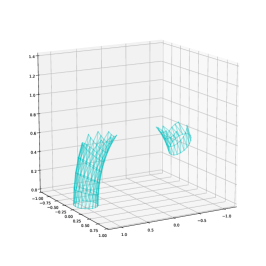
(b) Step 2

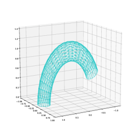
(c) Step 3

Figure 5: Example of filtration.

4.2 Constructing the persistent homology through harmonics

In this section, we present a construction of the $k$-persistent homology module $\{\mathcal{H}_{k}^{i},\hat{f}_{i}\}_{i\in\mathbb{N}}$ for coefficients in $\mathbb{R}$ through the space of $k$-harmonics. We call the persistence module $\{\mathcal{H}_{k}^{i},\hat{f}_{i}\}_{i\in\mathbb{N}}$ the harmonic persistence module.

After some preliminaries on the Hodge Laplacian operator, by means of the Hodge decomposition (Formula 3), for each index $i\in\mathbb{N}$, we retrieve the persistence module step of the harmonic persistence module. Afterwards, we introduce Algorithm 8 for retrieving the structure map $\hat{f}_{i}$ as the map, at $k$-harmonics level, ensuring the isomorphism of persistence modules between the $k$-persistent homology module $\{H_{k}^{i},\varphi_{i}\}$ and the harmonic persistence module $\{\mathcal{H}^{i}_{k},\hat{f}_{i}\}$ proven in Theorem 5. Notice that this construction, as it was for the case of general coefficients, can be distributed and performed in parallel for each $i\in\mathbb{N}$.

The Hodge Laplacian operator

Since $\mathbb{R}$ has characteristic equal to $0$, given a chain complex

$$\dots\overset{\partial_{k+2}}{\longrightarrow}C_{k+1}\overset{\partial_{k+1}}{\longrightarrow}C_{k}\overset{\partial_{k}}{\longrightarrow}C_{k-1}\overset{\partial_{k-1}}{\longrightarrow}\dots\overset{\partial_{2}}{\longrightarrow}C_{1}\overset{\partial_{1}}{\longrightarrow}C_{0}\overset{\partial_{0}}{\longrightarrow}0,$$

we fix an inner product $\langle\cdot,\cdot\rangle_{k}$ on each space of $k$-chains $C_{k}$ so that each operator $\partial_{k}$ has a well-defined adjoint operator $\partial^{*}_{k}$, i.e.,$\langle\partial_{k}(c),d\rangle_{k}=\langle c,\partial^{*}_{k}(d)\rangle_{k}$.

We consider the sequence $C^{*}$

$$\dots\overset{\partial^{*}_{k+2}}{\longleftarrow}C_{k+1}\overset{\partial^{*}_{k+1}}{\longleftarrow}C_{k}\overset{\partial^{*}_{k}}{\longleftarrow}C_{k-1}\overset{\partial^{*}_{k-1}}{\longleftarrow}\dots\overset{\partial^{*}_{2}}{\longleftarrow}C_{1}\overset{\partial^{*}_{1}}{\longleftarrow}C_{0}\overset{\partial^{*}_{0}}{\longleftarrow}0.$$

For $k\in\mathbb{N}$, the Hodge Laplacian in degree $k$ (Laplacian, for short) is the linear operator on $k$-chains $L_{k}:C_{k}\longrightarrow C_{k}$ given by

$$L_{k}:=\partial_{k+1}\partial^{*}_{k+1}+\partial^{*}_{k}\partial_{k}.$$ (15)

Constructing the harmonic step in parallel

For each index $i\in\mathbb{N}$, the step in the harmonic persistence module is given by the space of $k$-harmonics. The space of $k$-harmonics of a chain complex is the subspace of $C_{k}$

$$\mathcal{H}_{k}:=\ker(L_{k}).$$ (16)

Remark 5.

If $h\in\mathcal{H}_{k}$, then $h\in\ker(\partial_{k})$ and $h\in\ker(\partial_{k+1}^{*})$.

Indeed, both $\partial_{k}^{*}\partial_{k}$ and $\partial_{k+1}\partial^{*}_{k+1}$ are positive semidefinite, as $\langle c,\partial_{k}^{*}\partial_{k}c\rangle_{k}=$ $\langle\partial_{k}c,\partial_{k}c\rangle_{k}\geq 0$ and $\langle c,\partial_{k+1}\partial^{*}_{k+1}c\rangle_{k}=\langle\partial_{k+1}^{*}c,\partial^{*}_{k+1}c\rangle_{k}\geq 0$. Hence, $L_{k}$ is positive semidefinite, and $L_{k}c=0$ implies $\partial_{k}^{*}\partial_{k}c=0$ and $\partial_{k+1}\partial^{*}_{k+1}c=0$. Thus, $\langle\partial_{k}c,\partial_{k}c\rangle_{k}=0$ and $\langle\partial_{k+1}^{*}c,\partial^{*}_{k+1}c\rangle_{k}=0$.

Elements of $\ker(\partial_{k+1}^{*})$ are called $k$-cocycles. We refer to [18] for more details.

Before moving to the computation of the structure maps in the harmonic persistence module, we discuss some useful results relative to the single step $\mathcal{H}^{i}_{k}$.

First of all, the Hodge decomposition theorem states that:

Theorem 3.

For a chain complex $C$ and for every natural $k$,

$$C_{k}=\mathcal{H}_{k}\oplus\text{Im }(\partial_{k+1})\oplus\text{Im }(\partial_{k}^{*})$$

Moreover, this decomposition is orthogonal and $Z_{k}=\mathcal{H}_{k}\oplus\text{Im }(\partial_{k+1})$.

By Remark 5 , we can consider the homology class $[h]$ of an element $h\in\mathcal{H}_{k}$. As per Hodge theory ([11, 18]), it holds

Theorem 4.

The linear map $\psi_{k}:\mathcal{H}_{k}\longrightarrow H_{k}$ defined by $\psi_{k}(h)=[h]$ is an isomorphism.

Given the Hodge decomposition there is the orthogonal projection $\pi_{k}:Z_{k}\to\mathcal{H}_{k}$ that is equal to the identity on $\mathcal{H}_{k}$ and sends the elements of $B_{k}$ to zero.

Lemma 4.

For any $k$-cycle $z\in Z_{k}$, it holds $[z]=[\pi_{k}(z)]$ in $H_{k}$.

Proof.

Any $k$-cycle $z$ can be written uniquely as $h+b$, where $h\in\mathcal{H}_{k}$ and $b\in B_{k}$. Since $\pi_{k}$ sends boundaries to zero and it is the identity on $\mathcal{H}_{k}$, it holds $z-\pi_{k}(z)=h+b-h=b$, and therefore $z$ and $\pi_{k}(z)$ are in the same homology class. ∎

Remark 6.

If one chooses an orthonormal basis for the $k$-harmonics $\mathcal{H}_{k}$ and represent it via the matrix $V_{k}$ whose columns are the basis vectors, then the projection $\pi_{k}$ is represented by the matrix $V_{k}^{T}$.

Computing the harmonic structure map in parallel

In order to define the persistent homology with respect to harmonic representatives, we focus on the behavior of the harmonic subspace under the action of chain maps. On the one hand, we need to remark the following.

Remark 7.

A chain map $f:C\longrightarrow D$ does not restrict to a map between the harmonic subspaces $\mathcal{H}_{k}^{C}$ and $\mathcal{H}_{k}^{D}$.

Indeed, given an element $h\in\mathcal{H}_{k}^{C}$, the $k$-cycle $f(h)$ is not necessarily in $\mathcal{H}_{k}^{D}$. More precisely, $f(h)$ is necessarily a $k$-cycle but not necessarily a $k$-cocycle.

On the other hand, we can define a map $\hat{f}_{K}:\mathcal{H}_{k}^{C}\to\mathcal{H}_{k}^{D}$ in the following way. Consider the natural inclusion $i_{k}^{C}:\mathcal{H}_{k}^{C}\to C_{k}$ and the projection $\pi_{k}^{D}:D_{k}\to\mathcal{H}_{k}^{D}$. We define

$$\hat{f}_{k}=\pi_{k}^{D}f_{k}i_{k}^{C}.$$ (17)

Notice that the above definition corresponds to the general quotient map construction in Equation (27) of the Appendix A.

Algorithm 8 computes Equation (17) by applying Remark 6 the domain $C$ and the target $D$ to represent maps $i_{k}^{C}$ and $\pi_{k}^{D}$.

Consider now a sequence of chain complexes connected by linear maps as in the sequence (12). We get induced the following sequence of linear maps between $k$-harmonic spaces

Theorem 5.

The persistent homologies $\{H_{k,{(i)}},\tilde{f}_{k,{(i)}}\}_{i=0}^{n}$ and
$\{\mathcal{H}_{k,{(i)}},\hat{f}_{k,{(i)}}\}_{i=0}^{n}$ are isomorphic as persistence modules with coefficients in $\mathbb{R}$,

Proof.

It is enough to show that, for any chain map $f:C\longrightarrow D$, the following diagram commutes

That is, for any $h\in\mathcal{H}_{k}^{C}$, it must be $\tilde{f}_{k}(\psi_{k}^{C}(h))=\psi_{k}^{D}(\hat{f}_{k}(h))$. By the definition of $\tilde{f}_{k}$ and $\hat{f}_{k}$ the equality becomes $[f_{k}(h)]=[\pi_{k}^{D}(f_{k}(h))]$. Since $f_{k}(h)$ belongs to $Z_{k}^{D}$, the statements follows from Lemma 4.

∎

Input: Chain map $f_{k}:C_{k}(C)\to C_{k}(D)$, $V_{C}$ basis of $\ker(L_{k}(C_{k}(C)))$, $V_{D}$ basis of $\ker(L_{k}(C_{k}(D)))$ ;

Result: Matrix $\Phi$ representing $\hat{f}_{k}:\mathcal{H}_{k}(C)\to\mathcal{H}_{k}(D)$

$\Phi=V_{D}^{T}\cdot f_{k}\cdot V_{C}$;

return $(\Phi_{i})$

Algorithm 8 Induced map between Laplacian kernels

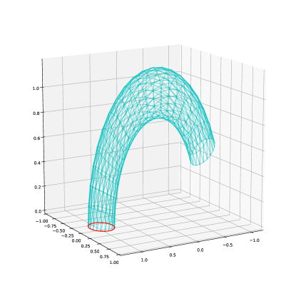
(a) Generator 1

(b) Generator 2

Figure 6: Generators, classical algorithm.

5 Conclusions and Future Works

In this work, we have introduced an algorithm for decomposing any persistence module, not necessarily a persistent homology module, into interval modules. We have discussed our method as supporting parallel and distributed implementations.
We have presented it into two versions: a general one and a specific one for the case of real coefficients where one can take advantage of the SVD matrix decomposition.
We have introduced the notion of interval basis as the persistence module analogue for the notion of minimal homogeneous generators of a graded module with coefficients in $\mathbb{F}[x]$. We have provided a proof of correctness of our approach which can be seen as an alternative and constructive proof of the Structure Theorem.

Afterwards, we have made explicit how to integrate our approach into the persistent homology pipeline, the main computational framework in TDA. Indeed, we have practically indicated how to obtain a persistent homology module out of a monotone sequence of chain complexes. Above all, we have remarked that each step and structure map in the module can be obtained independently, thus being suitable for parallel and distributed approaches.

Such an integration has offered interesting insights to be investigated further. For instance, it has made possible to geometrically locate the interval basis vectors onto a filtration of simplicial complexes. We have discussed simple examples to make comparisons with the classica generators obtained through the reduction algorithm [5]. We believe that the descriptive power of the interval basis deserves further study since it encodes implicitly the relations among evolving homology classes along a filtration.

As a last point to be addressed in the future, we have seen how working at persistence module level might be favorable for dealing with the persistence of harmonics. In particular, we have discussed how to overcome the non-functoriality of the harmonic forms by working at persistence module level. From the computational complexity point of view, we have shown how, for a persistence module, both our decomposition and our construction procedures can take advantage of having real coefficients. From the geometrical point of view, we have shown how the interval basis choice for generators applies to the harmonic case. Hence, our work contributes in combining harmonic generators into the persistent homology framework.

Appendix A Appendix - Categorical Aspects

A.1 Notes on linear maps of short exact sequences in the category of finite vector spaces

In this section, all spaces are finite vector spaces and all maps are linear maps.

Short exact sequences

A short exact sequence (s.e.s., for short) is a sequence of maps

(18)

such that, for each space in the sequence, the image of the map targeting the space and the kernel of the map which follows are equal.

In the category of finite vector spaces, a quotient space $Q=A/\sim$ of a space $A$ induces an s.e.s. where $K$ is the kernel of the quotient relation $\sim$, the map $s$ is the natural injection of $K$ into $A$, $q$ is the natural projection from $A$ to $A/\sim$. Since the category of finite vector spaces with linear maps is known to be an Abelian category (see Chapter VIII in [22]), the category admits kernel representations for surjective maps and quotient representations for injective maps. Hence, up to isomorphisms, a short exact sequence represents a quotient space. This motivates us in calling, given an s.e.s. such as the one in (18), the space $Q$ the quotient space, and the space $K$ the kernel space of the s.e.s.

Example 2.

An example of a short exact sequence is given by the $k$-homology space $H_{k}$ as a quotient of the $k$-cycle space $Z_{k}$ with kernel of the quotient relation given by the $k$-boundary space $B_{k}$:

where the arrow denotes the natural injection and the map $[\cdot]$ is the natural quotient projection defining the $k$-homology space (see Section 4).

Example 3.

Another relevant short exact sequence is the one involving the space of $k$-harmonics $\mathcal{H}_{k}$ introduced in Section 4.2. Indeed, the Theorem 4, as a corollary of the Hodge Decomposition Theorem 3, and the definition of the projection map $\pi_{k}$ satisfying Lemma 4 ensure the exactness of the following sequence

(19)

Consider the two short exact sequences as in the rows of the following diagram,

(20)

a map of short exact sequences is a tuple $(\varepsilon_{0},\varepsilon_{1},\varepsilon_{2})$ of maps such that the diagram in (20) commutes. An isomorphism of short exact sequences is a map of short sequences where each map is an isomorphism.

Lemma 5 (Splitting [17]).

For a short exact sequence

the following statements are equivalent:

1. there exists a surjective map such that

2. there exists an injective map such that

3. there exists an isomorphism such that $(\mbox{id}_{Q},h,\mbox{id}_{Q})$ is an isomorphisms of short exact sequences

   (21)

   where morphisms $\mbox{incl}_{1}$, $\mbox{proj}_{2}$ are the canonical inclusion and projection of the direct sum $\oplus$.

Remark 8.

In the category of finite vector spaces with linear maps, each short exact sequence admits a splitting, i.e. the sequence in the bottom row in (21) is a split sequence.

Indeed, this follows by noticing that any set of linearly independent vectors in a vector space can be extended to a basis.

Maps induced on quotient spaces by representatives

With respect to the notation in Diagram (20), we say that a map $\varepsilon:A\longrightarrow A^{\prime}$ is compatible with the short exact sequences if it satisfies $\varepsilon(s(A))\subseteq s^{\prime}(A^{\prime})$. In other words, a compatible map preserves kernels between the domain and the target sequences so that it is possible to induce maps on kernels and quotient spaces.

Remark 9.

If a map $\varepsilon:A\longrightarrow A^{\prime}$ is compatible with the short exact sequences in Diagram (20), then there exists only one map of short exact sequences $(\varepsilon_{|},\varepsilon,\tilde{\varepsilon})$ where

$$\varepsilon_{|}= p^{\prime}fs, p^{\prime}$$ with as in the splitting of case a) (22)

$$\tilde{\varepsilon}= q^{\prime}fr, r$$ with as in the splitting of case b). (23)

Indeed, the maps $\varepsilon_{|}$ and $\tilde{\varepsilon}$ are well defined and unique by the compatibility assumption. As for the existence, it is ensured by Remark 8.

Example 4.

An example of a map compatible with two short exact sequences is given by the map $f_{k}$ in the degree $k$ of a chain map (see Section 4). By homology functoriality, we have the following commutative diagram

(24)

where maps $f_{|}$ and $\tilde{f}$ satisfy Equation (22) and (23), respectively.

Indeed, homology functoriality depends on the map $f_{k}$ preserving $k$-cycles and $k$-boundaries. In particular for the map $\tilde{f}$ between quotient spaces, a choice of homology representative corresponds to a splitting map $r_{k}:H_{k}\longrightarrow Z_{k}$ satisfying case b) in Lemma 5.

This gives us a way of retrieving the map $\tilde{f}_{k}$ as

$$\tilde{f}_{k}=[\cdot]^{\prime}f_{k}r_{k}$$ (25)

for some choice $r_{k}$ of homology reprentatives, i.e., such that $[\cdot]r_{k}=\mbox{id}_{H_{k}}$.

Example 5.

Moreover, by homology functoriality, we get that the map $f_{k}$ is compatible with two short sequences like in Diagram (19) where we substitute the $k$-homology space with the $k$-harmonic space $\mathcal{H}_{k}$ and where, this time, we call $\hat{f}_{k}$ the map induced between quotient spaces

(26)

Indeed, the compatibility condition on the map $f_{k}$ depends on the natural inclusions $B_{k}\subseteq Z_{k}$ whereas the exactness of rows has already been discussed.

In particular, given a basis for the space of $k$-harmonics as a map $r_{k}:\mathcal{H}_{k}\longrightarrow Z_{k}$ as in the splitting of case b) in Lemma 5, we can express the map induced at harmonics level as follows

$$\hat{f}_{k}=\pi_{k}^{\prime}f_{k}r_{k}.$$ (27)

Maps induced on quotient spaces by split sequences

As a last remark, we express the Equations (23) and (22) of the maps induced on quotient and kernel terms in the case of split sequences satisfying case c) in Lemma 5 with respect to two given short exact sequences with the notation of the rows in Diagram (18). Let $\varepsilon$ be a map compatible with the two original short exact sequences with maps $\varepsilon_{|}$ and $\tilde{\varepsilon}$ induced on kernel and quotient spaces, respectively. We claim that the map $\varepsilon$ induces a map $\varepsilon^{*}$, that we call direct sum map, compatible with the two split sequences of case c) associated to the domain and target sequences

(28)

Indeed by assumption, we have two isomorphisms $h:K\oplus Q\longrightarrow A$ such that $qh=\mbox{proj}_{2}$ and $h^{\prime}:K^{\prime}\oplus Q^{\prime}\longrightarrow A^{\prime}$ such that $q^{\prime}h^{\prime}=\mbox{proj}_{2}$. We define $\varepsilon^{*}=h^{\prime-1}\varepsilon h$. It is easy to check that conditions $qh=\mbox{proj}_{2}$ and $q^{\prime}h^{\prime}=\mbox{proj}_{2}$ expressing the commuativity of Diagram (21) ensure that the maps $\varepsilon_{|}$ and $\tilde{\varepsilon}$ are the same as in Diagram (20). Hence the following remark holds.

Remark 10.

Given the direct sum map $\varepsilon^{*}$ of a compatible map $\varepsilon$ inducing maps $\varepsilon_{|}$ and $\tilde{\varepsilon}$ between kernel and quotient spaces respectively, we get that

$$\tilde{\varepsilon} =\mbox{proj}_{2}\varepsilon^{*}\mbox{incl}_{2}$$ (29)

$$\varepsilon_{|} =\mbox{proj}_{1}\varepsilon^{*}\mbox{incl}_{1},$$ (30)

where the tuple $(\varepsilon_{|},\varepsilon^{*},\tilde{\varepsilon})$ defines a map of short exact split sequences.

Appendix B Appendix - Preliminaries on simplicial complexes and persistent homology

In this appendix, we recall some basics in Simplicial Homology [17, 23, 21].

Our purpose is that of moving from the purely algebraic setting presented so far along the paper to the main input representation within the persistent homology pipeline, namely the notion of simplicial complex. (Geometric) simplicial complexes allow for representing geometric shapes into combinatorial and discrete terms. This way, a simplicial complex captures the topology of a shape into computable terms.

Here, we start by introducing the (abstract) definition of a simplicial complex. The relevance of the abstract point of view derives from its descriptive power. Indeed, not all datasets come associated with an embedding into a coordinate space. Nonetheless, those datasets might be endowed with the purely combinatorial structure of an abstract simplicial complex where the topology is given by pairwise and higher-order relations among data. The reader interested in the persistent homology setting is referred to the surveys [12, 15, 2, 24, 14].

Abstract simplicial complexes

An abstract simplicial complex $\Sigma$ on a finite set $V$ is a subset of the power set of $V$, with the property of being closed under restriction. An element of $\Sigma$ is called a simplex and if $\sigma\in\Sigma,\ \tau\subseteq\sigma$ then $\tau\in\Sigma$. Elements of $V$ are usually called vertices. Simplices of cardinality $p+1$ are called $p$-simplices. We also say a $p$-simplex has dimension $p$. We call the $p$-skeleton of $\Sigma$ the set of simplices of $\Sigma$ of dimension $\leq p$. If $\tau\subseteq\sigma$ we say that $\tau$ is a face of $\sigma$ and $\sigma$ is a coface of $\tau$. The dimension of a simplicial complex is defined as $\dim\Sigma:=\max\{\dim\sigma\ /\ \sigma\in\Sigma\}$.

Geometric simplicial complexes

Simplicial complexes have a natural geometric interpretation: a (geometric) $p$-simplex $\sigma$ is the convex hull of $p+1$ affinely independent points in the Euclidean space. As such, a 0-simplex is a point, a 1-simplex an edge, a 2-simplex a triangle, a 3-simplex a tetrahedron, and so on. Every abstract simplicial complex has a geometric realization (and actually many of them), i.e. a geometric simplicial complex to which it is homeomorphic. A realization of an abstract complex is denoted by $|\Sigma|$.

From simplicial complexes to chain complexes

For $\Sigma$ a simplicial complex and ${\mathbb{F}}$ any field, the $k^{th}$-chain space $C_{k}(\Sigma;{\mathbb{F}})$ of $\Sigma$ is defined as the ${\mathbb{F}}$-vector space generated by the oriented $k$-simplices of $\Sigma$ and such that $-\sigma$ coincides with the opposite orientation on $\sigma$. When clear from the context, we drop the indication of the base field to ease the notation. An element of $C_{k}(\Sigma)$ is called $k$-chain: it is a finite linear combination $\sum_{i}\eta_{i}[\sigma_{i}]$ with $\eta_{i}\in{\mathbb{F}}$.
Up to fixing an orientation for each $k$-simplex when $k>0$, and instead naturally when $k=0$, a canonical basis of $C_{k}(\Sigma)$ is given by the $k$-chains corresponding to the individual oriented $k$-simplices of $\Sigma$.

Chain spaces are instrumental in introducing a linear operator that expresses the above-mentioned adjacency relations across dimensions. The boundary operator is a linear map $\partial_{k}:C_{k}(\Sigma)\rightarrow C_{k-1}(\Sigma)$ that on an element of canonical basis corresponding to the oriented $k$-simplex $\sigma=[v_{0},\dots,v_{k}]$, is defined as:

$$\partial_{k}(\sigma):=\sum_{i=0}^{k}(-1)^{i}[v_{0},\dots,\hat{v}_{i},\dots,v_{k}],$$ (31)

where $\hat{v}_{i}$ means that vertex $v_{i}$ is omitted. It extends to the whole chain space by linearity.

Example 6.

The collection $C_{\bullet}=\{C_{k}\}_{k=0}^{\infty}$ along with the collection of boundary operators $\partial_{\bullet}$ defines a chain complex like the one introduced in Section 4.
Indeed, it is easy to check that $\partial_{k}\partial_{k+1}=0$, for all integers $k$.

Simplicial complexes and persistence modules

A simplicial complex $\Sigma$ can be made into a filtration of simplicial complexes (or a filtered simplicial complex) by taking a finite sequence of subcomplexes $\Sigma_{0}\subseteq\Sigma_{1}\subseteq\dots\subseteq\Sigma_{p}=\Sigma$, where a subcomplex is a subset and also a simplicial complex.
For any index $i=0,\dots,p$, define $C_{(i)}=\left(C_{k,(i)},\partial_{k,(i)}\right)$ to be the chain complex associated with the simplicial complex $\Sigma_{i}$ in the filtered complex. Notice that each inclusion induces a linear chain map $\iota_{k,(i)}:C_{k,(i)}\longrightarrow C_{k,(i+1)}$. Indeed, $\iota_{k,(i)}\partial_{k+1,k,(i)}=\partial_{k,(i)}\iota_{k+1,(i)}$. Hence, any filtered complex induces a (free) persistence module

(32)

and by applying the homology construction we get the associated persistent homology module

(33)

The sequences (32) and (33) correspond to the general sequences constructed in Formula (12) and (13) in Section 4 where the discussion was purely algebraic.

References

• [1] Ulrich Bauer, Michael Kerber and Jan Reininghaus β€œClear and Compress: Computing Persistent Homology in Chunks” In Topological Methods in Data Analysis and Visualization III, Mathematics and Visualization Springer, Cham, 2014, pp. 103–117
• [2] Gunnar Carlsson β€œTopology and data” In Bulletin of the American Mathematical Society 46.2, 2009, pp. 255–308
• [3] Gunnar Carlsson, Anjan Dwaraknath and Bradley J. Nelson β€œPersistent and Zigzag Homology: A Matrix Factorization Viewpoint” In arXiv preprint, 2021 arXiv:1911.10693
• [4] Gunnar Carlsson and Vin Silva β€œZigzag Persistence” In Foundations of Computational Mathematics 10.4 Springer, 2010, pp. 367–405
• [5] Gunnar Carlsson and Afra Zomorodian β€œComputing Persistent Homology” In Discrete & Computational Geometry 33.2, 2005, pp. 249–274
• [6] FrΓ©dΓ©ric Chazal, Vin Silva, Marc Glisse and Steve Oudot β€œThe Structure and Stability of Persistence Modules” Springer, 2016
• [7] Cecil Jose A. Delfinado and Herbert Edelsbrunner β€œAn incremental algorithm for Betti numbers of simplicial complexes on the 3-sphere” In Computer Aided Geometric Design 12.7 North-Holland, 1995, pp. 771–784
• [8] Tamal K. Dey, Fengtao Fan and Yusu Wang β€œComputing topological persistence for simplicial maps” In Proceedings of the Annual Symposium on Computational Geometry Association for Computing Machinery, 2014, pp. 345–354
• [9] Tamal K Dey, Tianqi Li and Yusu Wang β€œEfficient algorithms for computing a minimal homology basis” In Latin American Symposium on Theoretical Informatics, 2018, pp. 376–398 Springer
• [10] Stefania Ebli and Gard Spreemann β€œA notion of harmonic clustering in simplicial complexes” In Proceedings - 18th IEEE International Conference on Machine Learning and Applications, ICMLA 2019 Institute of ElectricalElectronics Engineers Inc., 2019, pp. 1083–1090 DOI: 10.1109/ICMLA.2019.00182
• [11] Beno Eckmann β€œHarmonische Funktionen und Randwertaufgaben in einem Komplex” In Commentarii Mathematici Helvetici 17.1 Springer, 1944, pp. 240–255
• [12] Herbert Edelsbrunner and John Harer β€œPersistent homologyβ€”a survey” In Surveys on Discrete and Computational Geometry 453, Contemporary Mathematics providence, RI: American Mathematical Society, 2008, pp. 257–282
• [13] Herbert Edelsbrunner, David Letscher and Afra Zomorodian β€œTopological persistence and simplification” In Discrete and Computational Geometry 28.4 Springer New York, 2002, pp. 511–533
• [14] Ulderico Fugacci, Sara Scaramuccia, Federico Iuricich and Leila De Floriani β€œPersistent homology: a step-by-step introduction for newcomers” In STAG: Smart Tools and Apps in Computer Graphics Eurographics Proceedings, 2016, pp. 1–10
• [15] Robert Ghrist β€œBarcodes: The persistent topology of data” In Bulletin of the American Mathematical Society 45.1, 2008, pp. 61–75
• [16] Marco Guerra, Alessandro De Gregorio, Ulderico Fugacci, Giovanni Petri and Francesco Vaccarino β€œHomological scaffold via minimal homology bases” In Scientific reports 11.1 NLM (Medline), 2021, pp. 5355 DOI: 10.1038/s41598-021-84486-1
• [17] Allen Hatcher β€œAlgebraic Topology” In Cambridge University Press 60 Cornell University, New York, 2002, pp. 147–288
• [18] Danijela Horak and JΓΌrgen Jost β€œSpectra of combinatorial Laplace operators on simplicial complexes” In Advances in Mathematics 244, 2013, pp. 303–336
• [19] Sara KaliΕ‘nik, Vitaliy Kurlin and Davorin LeΕ‘nik β€œA higher-dimensional homologically persistent skeleton” In Advances in Applied Mathematics 102 Elsevier, 2019, pp. 113–142
• [20] Michael Kerber and Hannah Schreiber β€œBarcodes of Towers and a Streaming Algorithm for Persistent Homology” In Discrete and Computational Geometry 61.4 Springer New York LLC, 2019, pp. 852–879
• [21] Dimitry Kozlov β€œCombinatorial algebraic topology” Springer Science & Business Media, 2007
• [22] Saunders Mac Lane β€œCategories for the Working Mathematician” 5.2, Graduate Texts in Mathematics Springer-Verlag New York, 1998
• [23] James R. Munkres β€œElements of algebraic topology” CRC Press, 2018
• [24] Alice Patania, Francesco Vaccarino and Giovanni Petri β€œTopological analysis of data” In EPJ Data Science 6.1 Springer Berlin Heidelberg, 2017
• [25] Rui Wang, Duc Duy Nguyen and Guo-Wei Wei β€œPersistent spectral graph” In International Journal for Numerical Methods in Biomedical Engineering 36.9 Wiley-Blackwell, 2020, pp. e3376 DOI: 10.1002/cnm.3376
• [26] Rui Wang, Rundong Zhao, Emily Ribando-Gros, Jiahui Chen, Yiying Tong and Guo-Wei Wei β€œHERMES: Persistent spectral graph software” In Foundations of Data Science 3.1 American Institute of Mathematical Sciences (AIMS), 2021, pp. 67 DOI: 10.3934/fods.2021006