Asynchronous Stochastic Optimization
Robust to Arbitrary Delays

Abstract

We consider stochastic optimization with delayed gradients where, at each time step $t$, the algorithm makes an update using a stale stochastic gradient from step $t-d_{t}$ for some arbitrary delay $d_{t}$. This setting abstracts asynchronous distributed optimization where a central server receives gradient updates computed by worker machines. These machines can experience computation and communication loads that might vary significantly over time. In the general non-convex smooth optimization setting, we give a simple and efficient algorithm that requires $O(\sigma^{2}/\epsilon^{4}+\tau/\epsilon^{2})$ steps for finding an $\epsilon$-stationary point $x$, where $\tau$ is the average delay $\smash{\frac{1}{T}\sum_{t=1}^{T}d_{t}}$ and $\sigma^{2}$ is the variance of the stochastic gradients. This improves over previous work, which showed that stochastic gradient decent achieves the same rate but with respect to the maximal delay $\max_{t}d_{t}$, that can be significantly larger than the average delay especially in heterogeneous distributed systems. Our experiments demonstrate the efficacy and robustness of our algorithm in cases where the delay distribution is skewed or heavy-tailed.

1 Introduction

Gradient-based iterative optimization methods are widely used in large-scale machine learning applications as they are extremely simple to implement and use, and come with mild computational requirements. On the other hand, in their standard formulation they are also inherently serial and synchronous due to their iterative nature. For example, in stochastic gradient descent (SGD), each step involves an update of the form $x_{t+1}=x_{t}-\eta g_{t}$ where $x_{t}$ is the current iterate, and $g_{t}$ is a (stochastic) gradient vector evaluated at $x_{t}$. To progress to the next step of the method, the subsequent iterate $x_{t+1}$ has to be fully determined by the end of step $t$ as it is required for future gradient queries. Evidently, this scheme has to wait for the computation of the gradient $g_{t}$ to complete (this is often the most computationally intensive part in SGD) before it can evaluate $x_{t+1}$.

In modern large scale machine learning applications, a direct serial implementation of gradient methods like SGD is overly costly, and parallelizing the optimization process over several cores or machines is desired. Perhaps the most common parallelization approach is via mini-batching, where computation of stochastic gradients is distributed across several worker machines that send updates to a parameter server. The parameter server is responsible for accruing the individual updates into a single averaged gradient, and consequently, updating the optimization parameters using this gradient.

While mini-batching is well understood theoretically (e.g., Lan, 2012; Dekel et al., 2012; Cotter et al., 2011; Duchi et al., 2012), it is still fundamentally synchronous in nature and its performance is adversely determined by the slowest worker machine: the parameter server must wait for all updates from all workers to arrive before it can update the model it maintains. This could cause serious performance issues in heterogeneous distributed networks, where worker machines may be subject to unpredictable loads that vary significantly between workers (due to different hardware, communication bandwidth, etc.) and over time (due to varying users load, power outages, etc.).

An alternative approach that has recently gained popularity is to employ asynchronous gradient updates (e.g., Nedić et al., 2001; Agarwal and Duchi, 2012; Chaturapruek et al., 2015; Lian et al., 2015; Feyzmahdavian et al., 2016); namely, each worker machine computes gradients independently of the other machines, possibly on different iterates, and sends updates to the parameter server in an asynchronous fashion. This implies the parameter server might be making stale updates based on delayed gradients taken at earlier, out-of-date iterates. While these methods often work well in practice, they have proven to be much more intricate and challenging to analyze theoretically than synchronous gradient methods, and overall our understanding of asynchronous updates remains lacking.

Recently, Arjevani et al. (2020) and subsequently Stich and Karimireddy (2020) have made significant progress in analyzing delayed asynchronous gradient methods. They have shown that in stochastic optimization, delays only affect a lower-order term in the convergence bounds. In other words, if the delays are not too large, the convergence rate of SGD may not be affected by the delays. (Arjevani et al., 2020 first proved this for quadratic objectives; Stich and Karimireddy, 2020 then proved a more general result for smooth functions.) More concretely, Stich and Karimireddy (2020) showed that SGD with a sufficiently attenuated step size to account for the delays attains an iteration complexity bound of the form

$$O\brk 3{\frac{\sigma^{2}}{\epsilon^{4}}+\frac{\tau_{\max}}{\epsilon^{2}}}$$ (1)

for finding an $\epsilon$-stationary point of a possibly non-convex smooth objective function (namely, a point at which the gradient is of norm $\leq\epsilon$). Here $\sigma^{2}$ is the variance of the noise in the stochastic gradients, and $\tau_{\max}$ is the maximal possible delay, which is also needed to be known a-priori for properly tuning the SGD step size. Up to the $\tau_{\max}$ factor in the second term, this bound is identical to standard iteration bounds for stochastic non-convex SGD without delays (Ghadimi and Lan, 2013).

While the bound in Eq. 1 is a significant improvement over previous art, it is still lacking in one important aspect: the dependence on the maximal delay could be excessively large in truly asynchronous environments, making the second term in the bound the dominant term. For example, in heterogeneous or massively distributed networks, the maximal delay is effectively determined by the single slowest (or less reliable) worker machine—which is precisely the issue with synchronous methods we set to address in the first place. Moreover, as Stich and Karimireddy (2020) show, the step size used to achieve the bound in Eq. 1 could be as much as $\tau_{\max}$-times smaller than that of without delays, which could severely impact performance in practice.

1.1 Contribution

We propose a new algorithm for stochastic optimization with asynchronous delayed updates, we call “Picky SGD,” that is significantly more robust than SGD, especially when the (empirical) distribution of delays is skewed or heavy-tailed and thus the maximal delay could be very large. For general smooth possibly non-convex objectives, our algorithm achieves a convergence bound of the form

$$O\brk 3{\frac{\sigma^{2}}{\epsilon^{4}}+\frac{\tau_{\mathrm{avg}}}{\epsilon^{2}}},$$

where now $\tau_{\mathrm{avg}}$ is the average delay in retrospect. This is a significant improvement over the bound in Eq. 1 whenever $\tau_{\mathrm{avg}}\ll\tau_{\mathrm{max}}$, which is indeed the case with heavy-tailed delay distributions. Moreover, Picky SGD is very efficient, extremely simple to implement, and does not require to know the average delay $\tau_{\mathrm{avg}}$ ahead of time for optimal tuning. In fact, the algorithm only relies on a single additional hyper-parameter beyond the step-size.

Notably, and in contrast to SGD as analyzed in previous work (Stich and Karimireddy, 2020), our algorithm is able to employ a significantly larger effective step size, and thus one could expect it to perform well in practice compared to SGD. Indeed, we show in experiments that Picky SGD is able to converge quickly on large image classification tasks with a relatively high learning rate, even when very large delays are introduced. In contrast, in the same setting, SGD needs to be configured with a substantially reduced step size to be able to converge at all, consequently performing poorly compared to our algorithm.

Finally, we also address the case where $f$ is smooth and convex, in which we give a close variant of our algorithm with an iteration complexity bound of the form

$$O\brk 3{\frac{\sigma^{2}}{\epsilon^{2}}+\frac{\tau_{\mathrm{avg}}}{\epsilon}}$$

for obtaining a point $x$ with $f(x)-f(x^{*})\leq\epsilon$ (where $x^{*}$ is a minimizer of $f$ over ${\mathbb{R}}^{d}$). Here as well, our rate matches precisely the one obtained by the state-of-the-art (Stich and Karimireddy, 2020), but with the dependence on the maximal delay being replaced with the average delay. For consistency of presentation, we defer details on the convex case to Appendix A and focus here on our algorithm for non-convex optimization.

Concurrently to this work, Aviv et al. (2021) derived similar bounds that depend on the average delay. Compared to our contribution, their results are adaptive to the smoothness and noise parameters, but on the other hand, are restricted to convex functions and their algorithms are more elaborate and their implementation is more involved.

1.2 Additional related work

For general background on distributed asynchronous optimization and basic asymptotic convergence results, we refer to the classic book by Bertsekas and Tsitsiklis (1997). Since the influential work of Niu et al. (2011), there has been significant interest in asynchronous algorithms in a related model where there is a delay in updating individual parameters in a shared parameter vector (e.g., (Reddi et al., 2015; Mania et al., 2017; Zhou et al., 2018; Leblond et al., 2018)). This is of course very different from our model, where steps use the full gradient vector in atomic, yet delayed, updates.

Also related to our study is the literature on Local SGD (e.g., Woodworth et al., 2020 and references therein), which is a distributed gradient method that perform several local (serial) gradient update steps before communicating with the parameter server or with other machines. Local SGD methods have become popular recently since they are used extensively in Federated Learning (McMahan et al., 2017). We note that the theoretical study in this line of work is mostly concerned with analyzing existing distributed variants of SGD used in practice, whereas we aim to develop and analyze new algorithmic tools to help with mitigating the effect of stale gradients in asynchronous optimization.

A related yet orthogonal issue in distribution optimization, which we do not address here, is reducing the communication load between the workers and servers. One approach that was recently studied extensively is doing this by compressing gradient updates before they are transmitted over the network. We refer to Alistarh et al. (2017); Karimireddy et al. (2019); Stich and Karimireddy (2020) for further discussion and references.

2 Setup and Basic Definitions

2.1 Stochastic non-convex smooth optimization

We consider stochastic optimization of a $\beta$-smooth (not necessarily convex) non-negative function $f$ defined over the $d$-dimensional Euclidean space ${\mathbb{R}}^{d}$. A function $f$ is said to be $\beta$-smooth if it is differentiable and its gradient operator is $\beta$-Lipschitz, that is, if $\norm{\nabla f(x)-\nabla f(y)}\leq\beta\norm{x-y}$ for all $x,y\in{\mathbb{R}}^{d}$. This in particular implies (e.g., (Nesterov, 2003)) that for all $x,y\in{\mathbb{R}}^{d}$,

$$f(y)\leq f(x)+\nabla f(x)\boldsymbol{\cdot}(y-x)+\frac{\beta}{2}\norm{y-x}^{2}.$$ (2)

We assume a stochastic first-order oracle access to $f$; namely, $f$ is endowed with a stochastic gradient oracle that given a point $x\in{\mathbb{R}}^{d}$ returns a random vector $\tilde{g}(x)$, independent of all past randomization, such that $\mathbb{E}[\tilde{g}(x)\mid x]=\nabla f(x)$ and $\mathbb{E}[\norm{\tilde{g}(x)-\nabla f(x)}^{2}\mid x]\leq\sigma^{2}$ for some variance bound $\sigma^{2}\geq 0$. In this setting, our goal is to find an $\epsilon$-stationary point of $f$, namely, a point $x\in{\mathbb{R}}^{d}$ such that $\|\nabla f(x)\|\leq\epsilon$, with as few samples of stochastic gradients as possible.

2.2 Asynchronous delay model

We consider an abstract setting where stochastic gradients (namely, outputs for invocations of the stochastic first-order oracle) are received asynchronously and are subject to arbitrary delays. The asynchronous model can be abstracted as follows. We assume that at each step $t$ of the optimization, the algorithm obtains a pair $(x_{t-d_{t}},g_{t})$ where $g_{t}$ is a stochastic gradient at $x_{t-d_{t}}$ with variance bounded by $\sigma^{2}$; namely, $g_{t}$ is a random vector such that $\mathbb{E}_{t}g_{t}=\nabla f(x_{t-d_{t}})$ and $\mathbb{E}_{t}\norm{g_{t}-\nabla f(x_{t-d_{t}})}^{2}\leq\sigma^{2}$ for some delay $0\leq d_{t}<t$. Here and throughout, $\mathbb{E}_{t}[\cdot]$ denotes the expectation conditioned on all randomness drawn before step $t$. After processing the received gradient update, the algorithm may query a new stochastic gradient at whatever point it chooses (the result of this query will be received with a delay, as above).

Few remarks are in order:

• We stress that the delays $d_{1},d_{2},\ldots$ are entirely arbitrary, possibly chosen by an adversary; in particular, we do not assume they are sampled from a fixed stationary distribution. Nevertheless, we assume that the delays are independent of the randomness of the stochastic gradients (and of the internal randomness of the optimization algorithm, if any).

• For simplicity, we assumed above that a stochastic gradient is received at every round $t$. This is almost without loss of generality: if at some round no feedback is observed, we may simply skip the round without affecting the rest of the optimization process (up to a re-indexing of the remaining rounds).

• Similarly, we will also assume that only a single gradient is obtained in each step; the scenario that multiple gradients arrive at the same step (as in mini-batched methods) can be simulated by several subsequent iterations in each of which a single gradient is processed.

3 The Picky SGD Algorithm

We are now ready to present our asynchronous stochastic optimization algorithm, which we call Picky SGD; see pseudo-code in Algorithm 1. The algorithm is essentially a variant of stochastic gradient descent, parameterized by a learning rate $\eta$ as well as a target accuracy $\epsilon$.

Algorithm 1 Picky SGD

1:  input: learning rate $\eta$, target accuracy $\epsilon$.

2:  for $t=1,\ldots,T$ do

3:     receive delayed stochastic gradient $g_{t}$ and point $x_{t-d_{t}}$ such that $\mathbb{E}_{t}[g_{t}]=\nabla f(x_{t-d_{t}})$.

4:     if $\norm{x_{t}-x_{t-d_{t}}}\leq\ifrac{\epsilon}{(2\beta)}$ then

5:        update: $x_{t+1}=x_{t}-\eta g_{t}$.

6:     else

7:        pass: $x_{t+1}=x_{t}$.

8:     end if

9:  end for

Picky SGD maintains a sequence of iterates $x_{1},\ldots,x_{T}$. At step $t$, the algorithm receives a delayed stochastic gradient $g_{t}$ that was computed at an earlier iterate $x_{t-d_{t}}$ (line 3). Then, in line 4, the algorithm tests whether $\norm{x_{t}-x_{t-d_{t}}}\leq\ifrac{\epsilon}{2\beta}$. Intuitively, this aims to verify whether the delayed (expected) gradient $\nabla f(x_{t-d_{t}})$ is “similar” to the gradient $\nabla f(x_{t})$ at the current iterate $x_{t}$; due to the smoothness of $f$, we expect that if $x_{t-d_{t}}$ is close to $x_{t}$, then also the corresponding gradients will be similar. If this condition holds true, the algorithm takes a gradient step using $g_{t}$ with step size $\eta$.

Our main theoretical result is the following guarantee on the success of the algorithm.

Theorem 1.

Suppose that Algorithm 1 is initialized at $x_{1}\in{\mathbb{R}}^{d}$ with $f(x_{1})\leq F$ and ran with

$$T\geq 500\beta F\brk 3{\frac{\sigma^{2}}{\epsilon^{4}}+\frac{\tau+1}{\epsilon^{2}}},\quad\eta=\frac{1}{4\beta}\min\brk[c]3{1,\frac{\epsilon^{2}}{\sigma^{2}}},$$

where $\tau$ be the average delay, i.e., $\tau=(\ifrac{1}{T})\sum_{t=1}^{T}d_{t}$. Then, with probability at least $\frac{1}{2}$, there is some $1\leq t\leq T$ for which $\norm{\nabla f(x_{t})}\leq\epsilon$.

Observe that the optimal step size in Theorem 1 is independent of the average delay $\tau$. This is important for two main reasons: (i) implementing the algorithm does not require knowledge about future, yet-to-be-seen delays; and (ii) even with very large delays, the algorithm can maintain a high effective step size.

We note that the guarantee of Theorem 1 is slightly different from typical bounds in non-convex optimization (e.g., the bounds appearing in the previous work Karimireddy et al. (2019)): our result claims about the minimal gradient norm of any iterate rather than the average gradient norm over the iterates. Arguably, this difference does not represent a very strong limitation: the significance of convergence bounds in non-convex optimization is, in fact, in that they ensure that one of the iterates along the trajectory of the algorithm is indeed an approximate critical point, and the type of bound we establish is indeed sufficient to ensure exactly that.

We further note that while the theorem above only guarantees a constant success probability, it is not hard to amplify this probability to an arbitrary $1-\delta$ simply by restarting the algorithm $O(\log(1/\delta))$ times (with independent stochastic gradients); with high probability, one of the repetitions will be successful and run through a point with gradient norm $\leq\epsilon$, which would imply the guarantee in the theorem with probability at least $1-\delta$.

4 Analysis

In this section we analyze Algorithm 1 and prove our main result. Throughout, we denote $x^{\prime}_{t}=x_{t-d_{t}}$ and let $N_{t}$ denote the noise vector at step $t$, namely $N_{t}=g_{t}-\nabla f(x^{\prime}_{t})$. Note that $\mathbb{E}\brk[s]{N_{t}\mid x_{t},x_{t}^{\prime}}=0$ and $\mathbb{E}\brk[s]{\norm{N_{t}}^{2}\mid x_{t},x_{t}^{\prime}}\leq\sigma^{2}$, since the iterates $x_{t},x_{t}^{\prime}$ are conditionally independent of the noise in $g_{t}$ as this gradient is obtained by the algorithm only at step $t$, after $x_{t},x_{t}^{\prime}$ were determined.

To prove Theorem 1, we will analyze a variant of the algorithm that will stop making updates once it finds a point with $\norm{\nabla f(x)}\leq\epsilon$ (and eventually fails otherwise). That is, if $\norm{x_{t}-x^{\prime}_{t}}>\ifrac{\epsilon}{2\beta}$ or $\norm{\nabla f(x_{t})}\leq\epsilon$ then $x_{t+1}=x_{t}$. Else, $x_{t+1}=x_{t}-\eta g_{t}$. This variant is impossible to implement (since it needs to compute the exact gradient at each step), but the guarantee of Theorem 1 is valid for this variant if and only if it is valid for the original algorithm: one encounters an $\epsilon$-stationary point if and only if the other does so.

First, we prove a simple technical lemma guaranteeing that whenever the algorithm takes a step, a large gradient norm implies a large decrease in function value. It is a variant of the classical “descent lemma,” adapted to the case where the gradient step is taken with respect to a gradient computed at a nearby point.

Lemma 2.

Fix $x,x^{\prime}\in{\mathbb{R}}^{d}$ with $\norm{x-x^{\prime}}\leq\ifrac{\epsilon}{2\beta}$ and $\norm{\nabla f(x^{\prime})}>\epsilon$. Let $N\in{\mathbb{R}}^{d}$ be a random vector with $\mathbb{E}\brk[s]{N\mid x,x^{\prime}}=0$ and $\mathbb{E}\brk[s]{\norm{N}^{2}\mid x,x^{\prime}}\leq\sigma^{2}$. Then,

$$\mathbb{E}\brk[s]{f\brk{x-\eta\brk{\nabla f(x^{\prime})+N}}}-\mathbb{E}f(x)\leq-\frac{\eta}{2}\mathbb{E}\norm{\nabla f(x^{\prime})}^{2}+\frac{\eta^{2}\beta}{2}\brk{\sigma^{2}+\mathbb{E}\norm{\nabla f(x^{\prime})}^{2}}.$$

In particular, for our choice of $\eta$, we have

$$\frac{\eta}{4}\mathbb{E}\norm{\nabla f(x^{\prime})}^{2}\leq\mathbb{E}f(x)-\mathbb{E}\brk[s]{f\brk 1{x-\eta\brk{\nabla f(x^{\prime})+N}}}.$$ (3)

Proof.

Using the smoothness of $f$ (Eq. 2), we have

$$f(x-\eta\brk{\nabla f(x^{\prime})+N})-f(x)\leq-\eta\nabla f(x)\boldsymbol{\cdot}\brk{\nabla f(x^{\prime})+N}+\tfrac{1}{2}\eta^{2}\beta\norm{\nabla f(x^{\prime})+N}^{2}.$$

Taking expectation over $N$ conditioned on $x,x^{\prime}$, we get

$$\mkern-36.0mu\mathbb{E}\brk[s]{f(x-\eta\brk{\nabla f(x^{\prime})+N})-f(x)\mid x,x^{\prime}}$$

$$\leq-\eta\nabla f(x)\boldsymbol{\cdot}\nabla f(x^{\prime})+\tfrac{1}{2}\eta^{2}\beta\brk{\|\nabla f(x^{\prime})\|^{2}+\sigma^{2}}$$

$$=-\eta\nabla f(x^{\prime})\boldsymbol{\cdot}\nabla f(x^{\prime})-\eta\nabla f(x^{\prime})\boldsymbol{\cdot}(\nabla f(x)-\nabla f(x^{\prime}))+\tfrac{1}{2}\eta^{2}\beta\brk{\norm{\nabla f(x^{\prime})}^{2}+\sigma^{2}}$$

$$\leq-\eta\|\nabla f(x^{\prime})\|^{2}+\eta\beta\|\nabla f(x^{\prime})\|\|x-x^{\prime}\|+\tfrac{1}{2}\eta^{2}\beta\brk{\|\nabla f(x^{\prime})\|^{2}+\sigma^{2}}$$

$$=\eta\brk{\beta\|\nabla f(x^{\prime})\|\|x-x^{\prime}\|-\|\nabla f(x^{\prime})\|^{2}}+\tfrac{1}{2}\eta^{2}\beta\brk{\|\nabla f(x^{\prime})\|^{2}+\sigma^{2}}.$$

Since $\epsilon\leq\|\nabla f(x^{\prime})\|$ then

$$\|x-x^{\prime}\|\leq\frac{\epsilon}{2\beta}\leq\frac{1}{2\beta}\norm{\nabla f(x^{\prime})},$$

and we have

$$\mathbb{E}\brk[s]!{f(x-\eta\brk{\nabla f(x^{\prime})+N})-f(x)\mid x,x^{\prime}}\leq-\frac{\eta}{2}\|\nabla f(x^{\prime})\|^{2}+\tfrac{1}{2}\eta^{2}\beta\brk{\sigma^{2}+\|\nabla f(x^{\prime})\|^{2}}.$$

If $\epsilon\geq\sigma$ then $\sigma^{2}\leq\norm{\nabla f(x^{\prime})}^{2}$. This, with $\eta=\ifrac{1}{4\beta}$, yields Eq. 3. If $\epsilon<\sigma$ and $\eta=\ifrac{\epsilon^{2}}{4\sigma^{2}\beta}$, then $\eta^{2}\leq\ifrac{\epsilon^{2}}{16\sigma^{2}\beta^{2}}$. Plugging that in instead, using $\norm{\nabla f(x^{\prime})}\geq\epsilon$, and taking expectations (with respect to $x,x^{\prime}$) gets us Eq. 3. ∎

We next introduce a bit of additional notation. We denote by $I_{t}$ the indicator of event that the algorithm performed an update at time $t$. Namely,

$$I_{t}=I\set!{\|x_{t}-x^{\prime}_{t}\|\leq\ifrac{\epsilon}{2\beta}~{}\;\text{and}\;\|\nabla f(x_{t})\|>\epsilon}.$$

Note that $I_{t}=1$ implies that $\|\nabla f(x_{s})\|\geq\epsilon$ for all $s=1,\ldots,t$. Further, we denote by $\Delta_{t}=f(x_{t})-f(x_{t+1})$ the improvement at time $t$. Since $f$ is non-negative and $f(x_{1})\leq F$, we have that for all $t$,

$$\sum_{i=1}^{t}\Delta_{i}=f(x_{1})-f(x_{t+1})\leq F.$$

Note that by Lemma 2 we have that $\mathbb{E}\Delta_{t}\geq 0$. The rest of the proof is split into two cases: $\sigma\leq\epsilon$, and $\sigma\geq\epsilon$.

4.1 Case (i): $\boldsymbol{\sigma\leq\epsilon}$

This regime is intuitively the “low noise” regime in which the standard deviation of the gradient noise, $\sigma$, is smaller than the desired accuracy $\epsilon$. We prove the following.

Lemma 3.

Suppose that $\sigma\leq\epsilon$ and the algorithm fails with probability $\geq\tfrac{1}{2}$. Then $T\leq\ifrac{128\beta F(\tau+1)}{\epsilon^{2}}$.

To prove the lemma above, we first show that the algorithm must make a significant number of updates, as shown by the following lemma.

Lemma 4.

If the algorithm fails, then the number of updates that it makes is at least $T/4(\tau+1)$.

Proof.

Consider $U_{2\tau}$, the number of steps $t$ for which the delay $d_{t}$ is at least $2\tau$. We must have $U_{2\tau}\leq T/2$ (otherwise the total sum of delays exceeds $\tau T$, contradicting the definition of $\tau$). On the other hand, let $k$ be the number of updates that the algorithm makes. Let $t_{1}<t_{2}<...<t_{k}$ be the steps in which an update is made. Denote $t_{0}=0$ and $t_{k+1}=T$. Now, fix $i$ and consider the steps at times $s_{n}=t_{i}+n$ for $n\in[1,2,\ldots,t_{i+1}-t_{i}-1]$. In all those steps no update takes place and $x_{s_{n}}=x_{t_{i}}$. We must have $d_{s_{n}}>n$ for all $n$ (otherwise $x_{t}=x_{t-d_{t}}$ for $t=s_{n}$ and an update occurs). In particular we have that $d_{s_{n}}\geq 2\tau$ in at least $t_{i+1}-t_{i}-1-2\tau$ steps in $[t_{i},t_{i+1}]$. Hence,

$$U_{2\tau}\geq\sum_{i=0}^{k-1}\brk{t_{i+1}-t_{i}-1-2\tau}=T-k(1+2\tau).$$

Finally, it follows that $T-k(1+2\tau)\leq T/2$ which implies $k\geq\frac{T}{4(\tau+1)}.$ ∎

Given the lemma above, we prove Lemma 3 by showing that if the algorithm fails, it makes many updates in all of which we have $\norm{\nabla f(x_{t})}>\epsilon$. By Lemma 2, this means that in the $T$ time steps of the algorithm, it must decrease the value of $f$ significantly. Since we start at a point in which $f(x_{1})\leq F$, we must conclude that $T$ cannot be too large.

Proof of Lemma 3.

Combining Eq. 3 with $\eta=1/(4\beta)$ and Lemma 4, we get that if the algorithm fails with probability $\geq\tfrac{1}{2}$ then

$$F \geq\sum_{t=1}^{T}\mathbb{E}\Delta_{t}\geq\frac{1}{16\beta}\sum_{t=1}^{T}\mathbb{E}\brk[s]{I_{t}\|\nabla f(x_{t})\|^{2}}\geq\frac{1}{16\beta}\mathbb{E}\brk[s]4{\sum_{t=1}^{T}I_{t}\|\nabla f(x_{t})\|^{2}}$$

$$\geq\frac{1}{32\beta}\mathbb{E}\brk[s]4{\sum_{t=1}^{T}I_{t}\|\nabla f(x_{t})\|^{2}\;\Bigg{|}\;\text{algorithm fails}}\geq\frac{\epsilon^{2}}{32\beta}\mathbb{E}\brk[s]4{\sum_{t=1}^{T}I_{t}\;\Bigg{|}\;\text{algorithm fails}}\geq\frac{\epsilon^{2}}{32\beta}\frac{T}{4(\tau+1)}.$$

This yields the lemma’s statement. ∎

4.2 Case (ii): $\boldsymbol{\sigma>\epsilon}$

This is the “high noise” regime. For this case, we prove the following guarantee for the convergence of our algorithm.

Lemma 5.

Assume that $\sigma>\epsilon$ and the algorithm fails with probability $\geq\tfrac{1}{2}$. Then,

$$\sum_{t=1}^{T}\mathbb{E}\Delta_{t}\geq\frac{T}{500\beta}\min\brk[c]3{\frac{\epsilon^{2}}{\tau},\frac{\epsilon^{4}}{\sigma^{2}}}.$$

In particular,

$$T\leq 500\beta F\brk 3{\frac{\tau}{\epsilon^{2}}+\frac{\sigma^{2}}{\epsilon^{4}}}.$$

This result is attained using the following observation. Consider the iterate of algorithm at time $t$, $x_{t}$, and the point at which the gradient was computed $x^{\prime}_{t}=x_{t-d_{t}}$. We claim that if the algorithm has not decreased the function value sufficiently during the interval $[t-d_{t},t-1]$, then it is likely to trigger a large decline in the function value at time $t$. Formally, either $\mathbb{E}\Delta_{t}$ is large, or $\sum_{i=t-d_{t}}^{t-1}\mathbb{E}\Delta_{i}$ is large. To show the claim, we first upper bound the distance $\norm{x_{t}-x^{\prime}_{t}}$ in terms of $\sum_{i=t-d_{t}}^{t-1}\mathbb{E}\Delta_{i}$, as shown by the following technical lemma.

Lemma 6.

For all $t$ and $k$, it holds that

$$\mathbb{E}\norm{x_{t}-x_{t+k}}\leq\sqrt{\frac{1}{\beta}\sum_{i=t}^{t+k-1}\mathbb{E}\Delta_{i}}+\frac{4}{\epsilon}\sum_{i=t}^{t+k-1}\mathbb{E}\Delta_{i}.$$

Proof.

We have

$$\mathbb{E}\|x_{t}-x_{t+k}\|=\eta\mathbb{E}\norm 4{\sum_{i=t}^{t+k-1}I_{i}\brk{\nabla f(x^{\prime}_{i})+N_{i}}}\leq\eta\mathbb{E}\norm 4{\sum_{i=t}^{t+k-1}I_{i}\nabla f(x^{\prime}_{i})}+\eta\mathbb{E}\norm 4{\sum_{i=t}^{t+k-1}I_{i}N_{i}}.$$

We continue bounding the second term above as follows:

$$\mathbb{E}\left\|\sum_{i=t}^{t+k-1}I_{i}N_{i}\right\| \leq\sqrt{\mathbb{E}\left\|\sum_{i=t}^{t+k-1}I_{i}N_{i}\right\|^{2}}$$

$$=\sqrt{\mathbb{E}\sum_{i=t}^{t+k-1}\sum_{j=t}^{t+k-1}I_{i}I_{j}N_{i}\cdot N_{j}}$$

$$=\sqrt{\mathbb{E}\sum_{i=t}^{t+k-1}I_{i}\|N_{i}\|^{2}} \mathbb{E}[N_{i}\mid I_{i},I_{j},N_{j}]=0 i>j$$ ( for )

$$\leq\sigma\sqrt{\mathbb{E}\sum_{i=t}^{t+k-1}I_{i}}$$

$$\leq\frac{\sigma}{\epsilon}\sqrt{\mathbb{E}\sum_{i=t}^{t+k-1}I_{i}\norm{\nabla f(x^{\prime}_{i})}^{2}} \norm{\nabla f(x^{\prime}_{i})}\geq\epsilon I_{i}=1$$ ( when )

$$\leq\frac{\sigma}{\epsilon}\sqrt{\frac{16\sigma^{2}\beta}{\epsilon^{2}}\,\sum_{i=t}^{t+k-1}\mathbb{E}\Delta_{i}} \eta=\ifrac{\epsilon^{2}}{4\beta\sigma^{2}}$$ (Eq. 3, )

$$=\frac{4\sigma^{2}}{\epsilon^{2}}\sqrt{\beta\sum_{i=t}^{t+k-1}\mathbb{E}\Delta_{i}}$$

$$=\frac{1}{\eta}\sqrt{\frac{1}{\beta}\sum_{i=t}^{t+k-1}\mathbb{E}\Delta_{i}}, \eta=\ifrac{\epsilon^{2}}{4\beta\sigma^{2}}$$ ()

and

$$\mathbb{E}\norm 4{\sum_{i=t}^{t+k-1}I_{i}\nabla f(x^{\prime}_{i})} \leq\sum_{i=t}^{t+k-1}\mathbb{E}I_{i}\norm{\nabla f(x^{\prime}_{i})}$$

$$\leq\frac{1}{\epsilon}\sum_{i=t}^{t+k-1}\mathbb{E}I_{i}\norm{\nabla f(x^{\prime}_{i})}^{2} \norm{\nabla f(x^{\prime}_{i})}\geq\epsilon I_{i}=1$$ ( when )

$$\leq\frac{4}{\epsilon\eta}\sum_{i=t}^{t+k-1}\mathbb{E}\Delta_{i}.$$ (Eq. 3)

This completes the proof. ∎

Given the lemma above, it is now clear that if $\sum_{i=t-d_{t}}^{t-1}\mathbb{E}\Delta_{i}$ is sufficiently small, then $\mathbb{E}\norm{x_{t}-x^{\prime}_{t}}\ll\ifrac{\epsilon}{\beta}$ which means that the algorithm is likely (with constant probability) to take a step at time $t$. This argument yields the following.

Corollary 7.

Assume that the algorithm fails with probability $\geq\tfrac{1}{2}$. If $\sum_{i=t-d_{t}}^{t-1}\mathbb{E}\Delta_{i}<\ifrac{\epsilon^{2}}{125\beta}$ then $\mathbb{E}\Delta_{t}\geq\ifrac{\epsilon^{4}}{64\sigma^{2}\beta}.$ In particular,

$$\mathbb{E}\Delta_{t}+\frac{1}{2\tau}\sum_{i=t-d_{t}}^{t-1}\mathbb{E}\Delta_{i}\geq\frac{1}{250\beta}\min\brk[c]3{\frac{\epsilon^{2}}{\tau},\frac{\epsilon^{4}}{\sigma^{2}}}.$$

Proof.

If $\sum_{i=t-d_{i}}^{t-1}\mathbb{E}\Delta_{i}<\ifrac{\epsilon^{2}}{125\beta},$ then $\mathbb{E}\|x_{t-d_{t}}-x_{t}\|\leq\ifrac{\epsilon}{8\beta}$ by Lemma 6. By a Markov inequality, with probability $\geq\tfrac{3}{4}$, we have $\|x_{t-d_{t}}-x_{t}\|\leq\ifrac{\epsilon}{2\beta}.$ Since the probability that $\|\nabla f(x_{t-d_{t}})\|>\epsilon$ is at least $\frac{1}{2}$, we get that $\mathbb{E}I_{t}\geq\frac{1}{4}$. By Lemma 2 this implies that

$$\mathbb{E}\Delta_{t}\geq\frac{1}{4}\cdot\frac{\epsilon^{2}\cdot\epsilon^{2}}{16\sigma^{2}\beta}=\frac{\epsilon^{4}}{64\sigma^{2}\beta},$$

which yields our claim. ∎

We now prove our main claim. We show that if the algorithm fails, then in all time steps in which $d_{t}\leq 2\tau$ (of which there are at least $T/2$), either the algorithm makes a substantial step, or it has made significant updates in the interval $[t-d_{t},t-1]$. In any case, the function value must necessarily decrease overall in the $T$ time steps of the algorithm, concluding that $T$ cannot be too large.

Proof of Lemma 5.

We have,

$$\sum_{t=1}^{T}\mathbb{E}\Delta_{t}\geq\sum_{t:d_{t}\leq 2\tau}\frac{1}{2\tau}\sum_{i=t-d_{t}}^{t-1}\mathbb{E}\Delta_{i}.$$

Hence, using Corollary 7,

$$\sum_{t=1}^{T}\mathbb{E}\Delta_{t} \geq\frac{1}{2}\sum_{t:d_{t}\leq 2\tau}\brk 4{\mathbb{E}\Delta_{t}+\frac{1}{2\tau}\sum_{i=t-d_{t}}^{t-1}\mathbb{E}\Delta_{i}}$$

$$\geq\abs!{\set{t:d_{t}\leq 2\tau}}\,\frac{1}{250\beta}\min\brk[c]3{\frac{\epsilon^{2}}{\tau},\frac{\epsilon^{4}}{\sigma^{2}}}$$

$$\geq\frac{T}{2}\,\frac{1}{250\beta}\min\brk[c]3{\frac{\epsilon^{2}}{\tau},\frac{\epsilon^{4}}{\sigma^{2}}}$$

$$=\frac{T}{500\beta}\min\brk[c]3{\frac{\epsilon^{2}}{\tau},\frac{\epsilon^{4}}{\sigma^{2}}},$$

where we used Markov’s inequality to show that $|\{t:d_{t}\leq 2\tau\}|\geq\frac{1}{2}T$. ∎

4.3 Concluding the proof

Proof of Theorem 1.

In the case $\sigma\leq\epsilon$, Lemma 3 implies that if $T>\ifrac{128\beta F(\tau+1)}{\epsilon^{2}}$ then the algorithms succeeds with probability greater than $1/2$, which yields the theorem in this case. Similarly, Lemma 5 gives our claim in the case when $\sigma>\epsilon$. ∎

5 Experiments

To illustrate the robustness and efficacy of Picky SGD, we present a comparison between the performance of SGD versus Picky SGD under various delay distributions. In particular, we show that Picky SGD requires significantly less iterations to reach a fixes goal and is more robust to varying delay distributions.

5.1 Setup

The main goal of our experimental setup is to be reproducible. For that end, the experimentation is done in two phases. First, we perform a simulation to determine the delay $d_{t}$ at each iteration without actually computing any gradients: this is done by simulating $N$ concurrent worker threads sharing and collectively advancing a global iteration number, where each worker repeatedly records the current global iteration number $t_{\text{start}}$, waits a random amount of time from a prescribed Poisson distribution, then records the new global iteration number $t=t_{\text{end}}$ and the difference $d_{t}=t_{\text{end}}-t_{\text{start}}$, and increases the global iteration number. This information (a delay schedule) is calculated once for each tested scheme (differing in the number of workers and random distribution, as detailed below), and is stored for use in the second phase.

In the second phase of the experiments, the algorithms SGD and Picky SGD are executed for each delay schedule. Here, at every iteration the gradient is computed (if needed) and is kept until its usage as dictated by the schedule (and then applied at the appropriate global iteration number). As a result of this configuration, we get a fully reproducible set of experiments, where the algorithms performance may be compared as they are executed over identical delay series of identical statistical properties.

We created four different delay schedules: A baseline schedule (A) using $N=10$ workers and sampling the simulated wait from a Poisson distribution (this schedule serves to compare Picky SGD and SGD in a setting of relatively small delay variance) and schedules (B) (C) and (D) all using $N=75$ workers and sampling the simulated wait from bi-modal mixtures of Poisson distributions of similar mean but increasing variance respectively. See Figure 2 in the appendix for an illustration of the delay distributions of the four delay schedules used.

All training is performed on the standard CIFAR-10 dataset (Krizhevsky, 2009) using a ResNet56 with $9$ blocks model (He et al., 2016) and implemented in TensorFlow (Abadi et al., 2015). We compare Picky SGD (Algorithm 1) to the SGD algorithm which unconditionally updates the state $x_{t}$ given the stochastic delayed gradient $g_{t}$ (recall that $g_{t}$ is the stochastic gradient at state $x_{t-d_{t}}$).

For both algorithms, instead of a constant learning rate $\eta$ we use a piecewise-linear learning rate schedule as follows: we consider a baseline $\eta_{0}$ piecewise-linear learning rate schedule that achieves optimal performance in a synchronous distributed optimization setting (that is, for $d_{t}\equiv 0)$ and search (for each of the four delay schedules and each algorithm – to compensate for the effects of delays) for the best multiple of the baseline rate and the best first rate-change point. Alternatively, we also used a cosine decay learning rate schedule (with the duration of the decay as meta parameters). Another meta-parameter we optimize is the threshold $\epsilon/(2\beta)$ in line 4 of Picky SGD. Batch size 64 was used throughout the experiments. Note that although use chose the threshold value $\ifrac{\epsilon}{2\beta}$ by an exhaustive search, in practice, a good choice can be found by logging the distance values during a typical execution and choosing a high percentile value. See Appendix C for more details.

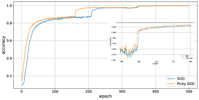
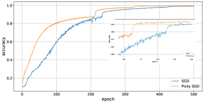
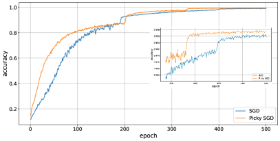
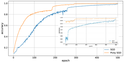
Figure 1: Accuracy trajectory (with a zoom-in on the tail of the convergence) over train epochs for the four delay schedules of Fig. 2, respectively: the key metrics (reported in Table 1) for each trajectory are epochs to reach 0.99 accuracy (the number of epochs required to reach the 0.99 accuracy mark) and the baseline learning rate multiplier $\ifrac{\eta}{\eta_{0}}$.

5.2 Results

The accuracy trajectory for the best performing combination of parameters of each algorithm for each of the four delay schedules is shown in Fig. 1 and summarized in Table 1. Clearly, Picky SGD significantly outperforms SGD in terms of the final accuracy and the number of epochs it takes to achieve it. We also emphasize that the generalization performance (that is, the evaluation accuracy as related to the training accuracy) was not observed to vary across delay schedules or the applied algorithms (see e.g., Fig. 4 in the appendix), and that the nature of the results is even more pronounced when using the alternative cosine decay learning rate schedule (see Fig. 5 in the appendix). Specific details of the meta parameters used, and additional performance figures are reported in Appendix B.

Table 1: Summary of the key metrics from Fig. 1, for each of the four delay schedules A, B, C, and D .

	Epochs to 0.99%		LR multiplier $(\ifrac{\eta}{\eta_{0}})$
	Picky SGD	SGD	Picky SGD	SGD
A	344	350	0.5	0.5
B	333	451	0.2	0.05
C	337	438	0.2	0.05
D	288	466	0.2	0.05

5.3 Discussion

We first observe that while the number of epochs it takes Picky SGD to reach the target accuracy mark is almost the same across the delay schedules (ranging from $288$ to $344$), SGD requires significantly more epochs to attain the target accuracy (ranging from $350$ up to $466$ for the highest variance delay schedule)—this is consistent with the average-delay bound dependence of Picky SGD (as stated in Theorem 1) compared to the max-delay bound dependence of SGD. Furthermore, the best baseline learning rate multiplier meta-parameter for Picky SGD is the same (0.2) across all high-variance delay schedules, while the respective meta parameter for SGD is significantly smaller (0.05) and sometimes varying, explaining the need for more steps to reach the target and evidence of Picky SGD superior robustness.

Acknowledgements

AD is partially supported by the Israeli Science Foundation (ISF) grant no. 2258/19. TK is partially supported by the Israeli Science Foundation (ISF) grant no. 2549/19, by the Len Blavatnik and the Blavatnik Family foundation, and by the Yandex Initiative in Machine Learning.

Appendix

Appendix A Picky SGD in the Convex Case

The algorithm for the convex case is a variant of Algorithm 1 and is displayed in Algorithm 2. In fact, the only difference from Algorithm 1 is in line 4 where the we use a threshold of $\sqrt{\ifrac{\epsilon}{8\beta}}$ instead of $\ifrac{\epsilon}{2\beta}$.

Algorithm 2 Picky SGD for Convex Objectives

1:  input: learning rate $\eta$, target accuracy $\epsilon$.

2:  for $t=1,\ldots,T$ do

3:     receive delayed stochastic gradient $g_{t}$ and point $x_{t-d_{t}}$ such that $\mathbb{E}_{t}[g_{t}]=\nabla f(x_{t-d_{t}})$.

4:     if $\norm{x_{t}-x_{t-d_{t}}}\leq\sqrt{\ifrac{\epsilon}{8\beta}}$ then

5:        update: $x_{t+1}=x_{t}-\eta g_{t}$.

6:     else

7:        pass: $x_{t+1}=x_{t}$.

8:     end if

9:     query stochastic gradient at $x_{t+1}$

10:  end for

Our guarantee for the algorithm is as follows.

Theorem 8.

Let $x_{\star}=\operatorname*{arg\,min}_{x\in{\mathbb{R}}^{d}}f(x)$. Suppose that Algorithm 2 is initialized at $x_{1}\in{\mathbb{R}}^{d}$ with $\norm{x_{1}-x_{\star}}\leq F$ and run with

$$T\geq 1600F^{2}\brk 3{\frac{\sigma^{2}}{\epsilon^{2}}+\frac{\beta(\tau+1)}{\epsilon}},\quad\eta=\min\brk[c]3{\frac{1}{16\beta},\frac{\epsilon}{8\sigma^{2}}},$$

where $\tau$ be the average delay, i.e., $\tau=(\ifrac{1}{T})\sum_{t=1}^{T}d_{t}$. Then, with probability at least $\frac{1}{2}$, there is some $1\leq t\leq T$ for which $f(x_{t})-f(x_{\star})\leq\epsilon$.

Note that we ensure the success of the algorithm only with probability $\frac{1}{2}$, but our guarantee can be easily converted to high probability in the same manner as done for Algorithm 1.

A.1 Analysis

The analysis proceeds similarly to that of Theorem 1. We analyze a variant of the algorithm that makes an update if $\norm{x_{t}-x^{\prime}_{t}}>\sqrt{\ifrac{\epsilon}{8\beta}}$ or $f(x_{t})-f(x_{\star})\leq\epsilon$ then $x_{t+1}=x_{t}$. Else, $x_{t+1}=x_{t}-\eta g_{t}$. As in the proof of Theorem 1, this variant is impossible to implement, but the guarantee of Theorem 8 is valid for this variant if and only if it is valid for the original algorithm.

We next introduce a bit of additional notation. We denote by $I_{t}$ the indicator of event that the algorithm performed an update at time $t$. Namely,

$$I_{t}=I\set!{\|x_{t}-x^{\prime}_{t}\|\leq\sqrt{\ifrac{\epsilon}{8\beta}}~{}\;\text{and}\;f(x_{t})-f(x_{\star})>\epsilon}.$$

Note that $I_{t}=1$ implies that $f(x_{s})-f(x_{\star})\geq\epsilon$ for all $s=1,\ldots,t$. Further, we denote by $\Delta_{t}=\norm{x_{t}-x_{\star}}^{2}-\norm{x_{t+1}-x_{\star}}^{2}$ the improvement at time $t$. Since we assume $\norm{x_{1}-x_{\star}}\leq F$, we have that for all $t$,

$$\sum_{i=1}^{t}\Delta_{i}=\norm{x_{1}-x_{\star}}^{2}-\norm{x_{t+1}-x_{\star}}^{2}\leq F^{2}.$$

Moreover, towards the proof we need the following that holds for any $\beta$-smooth convex function (see, e.g., Nesterov et al., 2018):

$$\frac{1}{2\beta}\norm{\nabla f(x)}^{2}\leq f(x)-f(x_{\star})\leq\nabla f(x)\boldsymbol{\cdot}\brk{f(x)-f(x_{\star})},\quad\text{for any }x\in{\mathbb{R}}^{d}.$$ (4)

The following lemma is an analog of Lemma 2 which shows that whenever the algorithm makes an update, the squared distance to the optimum $\norm{x_{t}-x_{\star}}^{2}$ decreases significantly.

Lemma 9.

Let $N\in{\mathbb{R}}^{d}$ be a random zero-mean vector with $\mathbb{E}\norm{N}^{2}\leq\sigma^{2}$. Fix $x,x^{\prime}\in{\mathbb{R}}^{d}$ with $\norm{x-x^{\prime}}\leq\ifrac{\epsilon}{4\beta}$ and $f(x^{\prime})-f(x_{\star})>\epsilon$. Then,

$$\mathbb{E}\brk[s]{\norm{x-\eta\brk{\nabla f(x^{\prime})+N}-x_{\star}}^{2}-\norm{x-x_{\star}}^{2}}\leq-\frac{\eta}{2}\norm{\nabla f(x^{\prime})}^{2}+\frac{\eta^{2}}{2}\brk{\sigma^{2}+\norm{\nabla f(x^{\prime})}^{2}}.$$

In particular, for our choice of $\eta$, we have

$$\mathbb{E}\brk[s]{\norm{x-\eta\brk{\nabla f(x^{\prime})+N}-x_{\star}}^{2}-\norm{x-x_{\star}}^{2}}\leq-\frac{\eta}{4}\brk{f(x^{\prime})-f(x_{\star})}.$$ (5)

Proof.

We have,

$$\norm{x-\eta\brk{\nabla f(x^{\prime})+N}-x_{\star}}^{2}-\norm{x-x_{\star}}^{2}=-\eta\brk{\nabla f(x^{\prime})+N}\boldsymbol{\cdot}(x-x_{\star})+\eta^{2}\norm{\nabla f(x^{\prime})+N}^{2}.$$

Taking expectation over $N$ we get

$$\mathbb{E}\brk[s]{\norm{x-\eta\brk{\nabla f(x^{\prime})+N}-x_{\star}}^{2}-\norm{x-x_{\star}}^{2}} \leq-\eta\nabla f(x^{\prime})\boldsymbol{\cdot}(x-x_{\star})+\eta^{2}\brk{\norm{\nabla f(x^{\prime})}^{2}+\sigma^{2}}$$

$$=-\eta\nabla f(x^{\prime})\boldsymbol{\cdot}(x^{\prime}-x_{\star})+\eta\nabla f(x^{\prime})\boldsymbol{\cdot}(x^{\prime}-x)+\eta^{2}\norm{\nabla f(x^{\prime})}^{2}+\eta^{2}\sigma^{2}$$

$$\leq-\eta\nabla f(x^{\prime})\boldsymbol{\cdot}(x^{\prime}-x_{\star})+\eta\norm{\nabla f(x^{\prime})}\norm{x^{\prime}-x}+\eta^{2}\norm{\nabla f(x^{\prime})}^{2}+\eta^{2}\sigma^{2}$$

$$\leq-\eta\brk{f(x^{\prime})-f(x_{\star})}+\eta\sqrt{2\beta\brk{f(x^{\prime})-f(x_{\star})}}\,\norm{x^{\prime}-x}$$

$$\qquad+2\beta\eta^{2}\brk{f(x^{\prime})-f(x_{\star})}+\eta^{2}\sigma^{2},$$

by using Eq. 4.

Now, since $\epsilon\leq f(x^{\prime})-f(x_{\star})$,

$$\|x-x^{\prime}\|\leq\sqrt{\frac{\epsilon}{8\beta}}\leq\sqrt{\frac{f(x^{\prime})-f(x_{\star})}{8\beta}},$$

and we have

$$\mathbb{E}\brk[s]{\norm{x-\eta\brk{\nabla f(x^{\prime})+N}-x_{\star}}^{2}-\norm{x-x_{\star}}^{2}}\leq-\frac{1}{2}\eta\brk{f(x^{\prime})-f(x_{\star})}+2\beta\eta^{2}\brk{f(x^{\prime})-f(x_{\star})}+\eta^{2}\sigma^{2}.$$

If $2\beta\epsilon\geq\sigma^{2}$ then $\sigma^{2}\leq 2\beta(f(x^{\prime})-f(x_{\star}))$. This, with $\eta=\ifrac{1}{16\beta}$, yields Eq. 5. If $2\beta\epsilon<\sigma^{2}$ and $\eta=\ifrac{\epsilon}{8\sigma^{2}}$. Plugging that in instead and using $f(x^{\prime})-f(x_{\star})\geq\epsilon$, gets us Eq. 5. ∎

Note that by Lemma 2 we have that $\mathbb{E}\Delta_{t}\geq 0$.

A.1.1 Case (i): ${\sigma^{2}\leq 2\beta\epsilon}$

We now handle the “low noise” and “high noise” regimes differently, beginning with the “low noise” regime. Recall that by Lemma 4 the algorithm makes at least $\Omega(\ifrac{T}{\tau})$ updates. This yields the following.

Lemma 10.

Suppose that $\sigma^{2}\leq 2\beta\epsilon$ and the algorithm fails with probability $\geq\tfrac{1}{2}$. Then $T\leq\ifrac{512\beta F^{2}(\tau+1)}{\epsilon}$.

Proof.

Combining Lemmas 4 and 9 we get that if the algorithm fails with probability $\geq\tfrac{1}{2}$ then

$$F^{2} \geq\sum_{t=1}^{T}\mathbb{E}\Delta_{t}$$

$$\geq\frac{1}{64\beta}\mathbb{E}\brk[s]4{\sum_{t=1}^{T}I_{t}\brk{f(x_{t})-f(x_{\star})}}$$

$$\geq\frac{1}{128\beta}\mathbb{E}\brk[s]4{\sum_{t=1}^{T}I_{t}\brk{f(x_{t})-f(x_{\star})}\;\Bigg{|}\;\text{algorithm fails}}$$

$$\geq\frac{\epsilon}{128\beta}\mathbb{E}\brk[s]4{\sum_{t=1}^{T}I_{t}\;\Bigg{|}\;\text{algorithm fails}}$$

$$\geq\frac{\epsilon}{128\beta}\frac{T}{4(\tau+1)}.\qed$$

A.1.2 Case (ii): ${\sigma^{2}>2\beta\epsilon}$

This is the “high noise” regime. For this case, we prove the following guarantee for the convergence of our algorithm.

Lemma 11.

Assume that $\sigma^{2}>2\beta\epsilon$ and the algorithm fails with probability $\geq\tfrac{1}{2}$. Then,

$$\sum_{t=1}^{T}\mathbb{E}\Delta_{t}\geq\frac{T}{1600}\min\brk[c]3{\frac{\epsilon}{\tau\beta},\frac{\epsilon^{2}}{\sigma^{2}}}.$$

In particular,

$$T\leq 1600F^{2}\brk 3{\frac{\tau\beta}{\epsilon}+\frac{\sigma^{2}}{\epsilon^{2}}}.$$

Similarly to Lemma 5, this result is attained by showing that either $\mathbb{E}\Delta_{t}$ is large, or $\sum_{i=t-d_{t}}^{t-1}\mathbb{E}\Delta_{i}$ is large. To prove the claim, we first upper bound the distance $\norm{x_{t}-x^{\prime}_{t}}$ in terms of $\sum_{i=t-d_{t}}^{t-1}\mathbb{E}\Delta_{i}$, as shown by the following lemma.

Lemma 12.

For all $t$ and $k$, it holds that

$$\mathbb{E}\norm{x_{t}-x_{t+k}}\leq\sqrt{\sum_{i=t}^{t+k-1}\mathbb{E}\Delta_{i}}+\sqrt{\frac{32\beta}{\epsilon}}\sum_{i=t}^{t+k-1}\mathbb{E}\Delta_{i}.$$

Proof.

We have

$$\mathbb{E}\|x_{t}-x_{t+k}\|=\eta\mathbb{E}\norm 4{\sum_{i=t}^{t+k-1}I_{i}\brk{\nabla f(x^{\prime}_{i})+N_{i}}}\leq\eta\mathbb{E}\norm 4{\sum_{i=t}^{t+k-1}I_{i}\nabla f(x^{\prime}_{i})}+\eta\mathbb{E}\norm 4{\sum_{i=t}^{t+k-1}I_{i}N_{i}}.$$

We continue bounding the second term above as follows:

$$\mathbb{E}\left\|\sum_{i=t}^{t+k-1}I_{i}N_{i}\right\| \leq\sqrt{\mathbb{E}\left\|\sum_{i=t}^{t+k-1}I_{i}N_{i}\right\|^{2}}$$

$$=\sqrt{\mathbb{E}\sum_{i=t}^{t+k-1}\sum_{j=t}^{t+k-1}I_{i}I_{j}N_{i}\cdot N_{j}}$$

$$=\sqrt{\mathbb{E}\sum_{i=t}^{t+k-1}I_{i}\|N_{i}\|^{2}} \mathbb{E}[N_{i}\mid I_{i},I_{j},N_{j}]=0 i>j$$ ( for )

$$\leq\sqrt{\sigma^{2}\mathbb{E}\sum_{i=t}^{t+k-1}I_{i}}$$

$$\leq\sqrt{\frac{\sigma^{2}}{\epsilon}\mathbb{E}\sum_{i=t}^{t+k-1}I_{i}\brk{f(x^{\prime}_{i})-f(x_{\star})}} f(x^{\prime}_{i})-f(x_{\star})\geq\epsilon I_{i}=1$$ ( when )

$$\leq\sqrt{\frac{\sigma^{2}}{\epsilon}\cdot\frac{32\sigma^{2}}{\epsilon}\,\sum_{i=t}^{t+k-1}\mathbb{E}\Delta_{i}}$$ (Eq. 5)

$$\leq\frac{8\sigma^{2}}{\epsilon}\sqrt{\sum_{i=t}^{t+k-1}\mathbb{E}\Delta_{i}}$$

$$=\frac{1}{\eta}\sqrt{\sum_{i=t}^{t+k-1}\mathbb{E}\Delta_{i}}, \eta=\ifrac{\epsilon}{8\sigma^{2}}$$ ()

and

$$\mathbb{E}\norm 4{\sum_{i=t}^{t+k-1}I_{i}\nabla f(x^{\prime}_{i})} \leq\sum_{i=t}^{t+k-1}\mathbb{E}I_{i}\norm{\nabla f(x^{\prime}_{i})}$$

$$\leq\sum_{i=t}^{t+k-1}\mathbb{E}I_{i}\sqrt{2\beta\brk{f(x^{\prime}_{i})-f(x_{\star})}} f \beta$$ ( convex and -smooth)

$$\leq\sqrt{\frac{2\beta}{\epsilon}}\sum_{i=t}^{t+k-1}\mathbb{E}I_{i}\brk{f(x^{\prime}_{i})-f(x_{\star})} f(x^{\prime}_{i})-f(x_{\star})\geq\epsilon I_{i}=1$$ ( when )

$$\leq\sqrt{\frac{32\beta}{\epsilon}}\cdot\frac{1}{\eta}\sum_{i=t}^{t+k-1}\mathbb{E}\Delta_{i}.$$ (Eq. 5)

This completes the proof. ∎

Given the lemma above, it is now clear that if $\sum_{i=t-d_{t}}^{t-1}\mathbb{E}\Delta_{i}$ is sufficiently small, then $\mathbb{E}\norm{x_{t}-x^{\prime}_{t}}\ll\sqrt{\frac{\epsilon}{\beta}}$ which means that the algorithm is likely (with constant probability) to take a step at time $t$. This argument yields the following.

Corollary 13.

Assume that the algorithm fails with probability $\geq\tfrac{1}{2}$. If $\sum_{i=t-d_{t}}^{t-1}\mathbb{E}\Delta_{i}<\ifrac{\epsilon}{400\beta}$ then $\mathbb{E}\Delta_{t}\geq\ifrac{\epsilon^{2}}{128\sigma^{2}}.$ In particular,

$$\mathbb{E}\Delta_{t}+\frac{1}{2\tau}\sum_{i=t-d_{t}}^{t-1}\mathbb{E}\Delta_{i}\geq\frac{1}{800}\min\brk[c]3{\frac{\epsilon}{\tau\beta},\frac{\epsilon^{2}}{\sigma^{2}}}.$$

Proof.

If $\sum_{i=t-d_{i}}^{t-1}\mathbb{E}\Delta_{i}<\ifrac{\epsilon}{400\beta},$ then $\mathbb{E}\|x_{t-d_{t}}-x_{t}\|\leq\sqrt{\ifrac{\epsilon}{128\beta}}$ by Lemma 12. By a Markov inequality, with probability $\geq\tfrac{3}{4}$, we have $\|x_{t-d_{t}}-x_{t}\|\leq\sqrt{\ifrac{\epsilon}{8\beta}}.$ Since the probability that $f(x_{t-d_{t}})-f(x_{\star})>\epsilon$ is at least $\frac{1}{2}$, we get that $\mathbb{E}I_{t}\geq\frac{1}{4}$. Finally, by Lemma 9 this implies that

$$\mathbb{E}\Delta_{t}\geq\frac{1}{4}\cdot\frac{\epsilon}{32\sigma^{2}}\cdot\epsilon=\frac{\epsilon^{2}}{128\sigma^{2}}\geq\frac{\epsilon^{2}}{800\sigma^{2}},$$

which yields our claim. ∎

We now prove our main claim.

Proof of Lemma 11.

We have,

$$\sum_{t=1}^{T}\mathbb{E}\Delta_{t}\geq\sum_{t:d_{t}\leq 2\tau}\frac{1}{2\tau}\sum_{i=t-d_{t}}^{t-1}\mathbb{E}\Delta_{i}.$$

Hence, using Corollary 13,

$$\sum_{t=1}^{T}\mathbb{E}\Delta_{t} \geq\frac{1}{2}\sum_{t:d_{t}\leq 2\tau}\brk 4{\mathbb{E}\Delta_{t}+\frac{1}{2\tau}\sum_{i=t-d_{t}}^{t-1}\mathbb{E}\Delta_{i}}\geq\abs!{\set{t:d_{t}\leq 2\tau}}\,\frac{1}{800}\min\brk[c]3{\frac{\epsilon}{\tau\beta},\frac{\epsilon^{2}}{\sigma^{2}}}\geq\frac{T}{2}\cdot\frac{1}{800}\min\brk[c]3{\frac{\epsilon}{\tau\beta},\frac{\epsilon^{2}}{\sigma^{2}}}$$

$$=\frac{T}{1600}\min\brk[c]3{\frac{\epsilon}{\tau\beta},\frac{\epsilon^{2}}{\sigma^{2}}},$$

where we used Markov’s inequality to show that $|\{t:d_{t}\leq 2\tau\}|\geq\frac{1}{2}T$. ∎

A.1.3 Concluding the proof

Proof of Theorem 8.

In the case $\sigma^{2}\leq 2\beta\epsilon$, Lemma 10 implies that if $T>\ifrac{512\beta F^{2}(\tau+1)}{\epsilon}$, then the algorithms succeeds with probability greater than $1/2$, which yields the theorem in this case. Similarly, Lemma 11 gives our claim in the case when $\sigma^{2}>2\beta\epsilon$. ∎

Appendix B Details of Experiments

B.1 Simulation method

In this section, we describe in detail the simulation environment that we used to compare the performance of distributed optimization algorithms under various heterogeneous distributed computation environments. Our simulation environment has two components: One, for generating the order in which the gradients are applied to the parameter state (see Algorithm 4, Generate Async Sequence) and another that given that order carries out the distributed optimization computation (sequentially, in a deterministic manner, see Algorithm 5, Simulate Async).

B.1.1 Generate Async Sequence

We consider a sequential distributed computation, where a shared state is updated by concurrent workers, and the update depends on the state history alone - that is, the update at state $S_{w}$ (at stage $w$, where $w=1\ldots T$) is a function of the state trajectory $S_{0},\ldots S_{w}$. Specifically, we address the case where the update is a function of a single state $S_{r}(w),\ \ r(w)\leq w$, from the trajectory. Crucially, the sequence $\{r(w)\}_{w=1\ldots T}$ uniquely determines the outcome $S_{T}$ of the computation. This setting captures a distributed gradient descent computation, where the gradient applied at state $S_{w}$ was computed at state $S_{r(w)}$. Indeed, up to data batching order, different optimization algorithms (SGD and Picky SGD, in our case) may be compared in a deterministic manner over the same generated sequence $\{r(w)\}_{w=1\ldots T}$, of certain predefined statistical properties.

We generate a sequence $Q=\{(r(w),w)\}_{w=1\ldots T}$ in Algorithm 4 by simulating concurrent workers that share a state $S$. Each worker (performing Algorithm 3), at each iteration creates a pair $(r,w)$ appended to $Q$ as follows: instead of actually performing the (gradient) computation, the worker merely records the state $r\leftarrow S$, waits for a random period, records the state again $w\leftarrow S$ and advances it (note that during the wait, the shared state may have been advanced by another worker). Note that the nature of the random wait determines the statistical properties of the generated sequence $Q$.

Algorithm 3 Generate Async Sequence - Worker

1:  shared variables: stage $S$, sequence $Q$, tasks queue $T$.

2:  while $T>0$ do

3:     $T\leftarrow T-1$

4:     $r\leftarrow S$

5:     Wait for a random period {gradient computation}

6:     $w\leftarrow S$, $S\leftarrow S+1$ {atomically}

7:     Wait for a random period {gradient update}

8:     $Q$.append($[r,w]$)

9:  end while

Algorithm 4 Generate Async Sequence

1:  input: number of workers $n$, number of steps $t$,

2:  Initialize shared variables: stage $S\leftarrow 0$, sequence $Q\leftarrow[]$, tasks queue $T\leftarrow t$.

3:  spawn $n$ workers.

4:  wait until $T=0$.

5:  return Sorted $Q$.

B.1.2 Simulate Async

Given a sorted sequence $Q=\{(r(w),w)\}_{w=1\ldots T}$, Algorithm 5 simulates the distributed optimization computation (of the state $X$ of a given model $M$) by sequentially considering pairs $(r,w)$ from $Q$.

The algorithm maintains a computation stage $S$, a map $G$, where $G[r]$ holds the gradient $g$ computed at stage $r$ (and the state $x$ for which the gradient was computed), and a map $F$, where $F[w]$ is the stage $r$ in which the gradient (to be applied at stage $w$) was computed.

For each pair $(r,w)$ in $Q$, the algorithm updates the map $F$ accordingly, and then, as long as the computation stage $S<r$, uses the information in the maps $G$ and $F$ to apply gradients to the computation state $X$ accordingly and advance the stage $S$, until it reaches $r$. The gradients are applied through the optimization algorithm (i.e., SGD or Picky SGD) which is passed as an input to the simulation. After the above catch up phase, the gradient at stage $r$ (Note that at this point $r=S$) is computed (this only happens for the first appearance of $r$) using a batch sampled from the input data set $D$, and the map $G$ is updated accordingly with the computed gradient $g$ and the computation state $X$.

Note that during the catch up phase, since $Q$ is sorted, if $r>S$ then $F[S]=r^{\prime}<S<r$ so the gradient at $r^{\prime}$ was already computed in a previous iteration (at the first time $r^{\prime}$ appeared in a pair $(r^{\prime},S)$ in $Q$). Moreover, $F[S]$ was updated at that same previous iteration, establishing correctness.

Algorithm 5 Simulate Async

1:  input: Sorted Sequence $Q$. Model $M$ with state $X$ to be optimized using algorithm $Alg$ over train data $D$.

2:  Initialize variables: computation stage $S\leftarrow 0$, gradients map $G\leftarrow\{\}$, apply stage map $F\leftarrow\{\}$.

3:  for $[r,w]$ in $Q$ do

4:     $F[w]\leftarrow r$.

5:     while $S<r$ do

6:        $g,x\leftarrow G[(F[S],S)]$

7:        $X\leftarrow$ $Alg$ apply gradient ($g$, computed at state $x$).

8:        $S\leftarrow S+1$

9:     end while

10:     $d\leftarrow$ data batch from $D$

11:     $g\leftarrow$ model $M$ gradient at $X$ for data batch $d$.

12:     $G[(S,w)]\leftarrow[g,X]$

13:  end for

14:  return $X$ {optimal state for $M$ over data set $D$ as computed by $Alg$}.

B.2 Experiments settings

B.2.1 Generated sequences

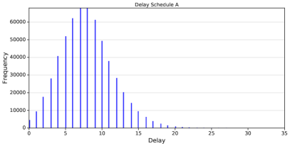
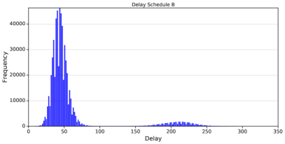
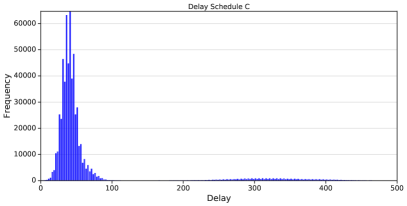
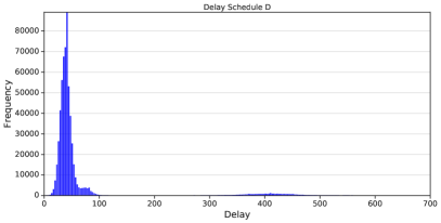
Figure 2: Delay histograms, derived from the delay schedules created for a total of 750 training epochs of CIFAR-10. (A) is the baseline schedule, while (B) (C) and (D) where created with increasing delay variance.

We used Algorithm 4 to generate four schedules with different statistical properties by varying the number of workers simulated and the sampled wait period distributions as follows: For schedule $A$ we used $n=10$ workers and Poisson distribution $P$. For the other schedules ($B$, $C$, and $D$) we simulated $75$ workers and used for each schedule a weighted mixture of two Poisson distributions: $P$ with probability $0.92$ and $150P$ with probability $0.08$ for schedule $B$. $P$ with probability $0.935$ and $240P$ with probability $0.065$ for schedule $C$. And $P$ with probability $0.95$ and $330P$ with probability $0.05$ for schedule $D$. In all schedules we used parameter $4.06$ for the Poisson distribution $P$. Finally, in Algorithm 3, we scaled the second wait by $0.2$ to reflect the relatively longer time required for gradient computation (compared to the time required for updating the state). The four delay schedules are illustrated in Fig. 2.

B.2.2 Meta parameters and further results

The baseline for the learning rate schedule we used is the one chosen for synchronous optimization of the same data set and model. It starts at a constant rate of $0.05$ and scaled down by $0.1$ at three (fixed upfront) occasions. We used the accuracy achieved at those points ($0.93,0.98,0.99$) to define a baseline learning rate schedule $\eta_{0}$ that behaves the same, but the accuracy of the first rate change being a meta-parameter $R$. We used values from $\{0.8,0.84,0.88,0.93$, $0.96\}$ for $R$. In addition, the baseline learning rate is further scaled by a meta parameter $K$ (The learning rate multiplier $\ifrac{\eta}{\eta_{0}}$). Values from $\{0.01,0.02,0.05,0.2,0.5,1.0,2.0\}$ were explored for $K$. Finally, and only for Picky SGD, we explored values of the threshold $\ifrac{\epsilon}{2\beta}$ in Algorithm 1. We aligned changes in the threshold together with the changes in the learning rate (effectively reducing the target accuracy approximation $\epsilon$), and explored thresholds of the form $A\sqrt{\eta_{0}}$ for values of $A$ in $\{1,3,6,9,12\}$.

All in all, for every constellation of the meta parameters $R$, $K$, and $A$, we run Algorithm 5 for SGD and for Picky SGD. The best performing constellation of SGD is compared with the best performing constellation of Picky SGD. Fig. 1 compares the performance trajectory for each of the four delay schedules generated by Algorithm 4. Fig. 3 is a comparison of the top three performing constellations of each of the optimization algorithms, further illustrating the robustness and superiority of Picky SGD over SGD. Table 1 and Fig. 4 details the eventual evaluation set performance and trajectory (respectively), for each optimization algorithm and each delay schedule, demonstrating the improved generalization for Picky SGD in all delay schedules.

	Test		Train
	Picky SGD	SGD	Picky SGD	SGD
A	92.98	92.56	99.87	99.82
B	91.82	89.64	99.62	99.25
C	92.12	90.09	99.66	99.23
D	91.80	90.15	99.61	99.22

Table 2: Eventual (top-1) accuracy of the experiments in Fig. 1 for train and evaluation data sets.

Finally, we compared the performance of Picky SGD to that of SGD for an alternative learning rate schedule - cosine decay. Using the learning rate decay duration (in epochs) as a meta parameter with values ranging over {$150,180,240,300,360$}. The training accuracy trajectories of the top 3 meta-parameters constellations of Picky SGD and SGD for the four delay schedules are illustrated in Fig. 5, showing an even more pronounced performance gap in favor of Picky SGD, mainly regarding the time to reach the 0.99 accuracy mark and robustness.

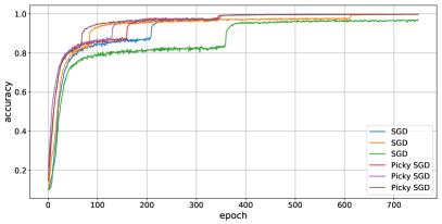
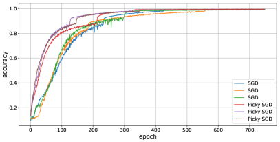
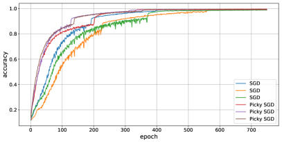
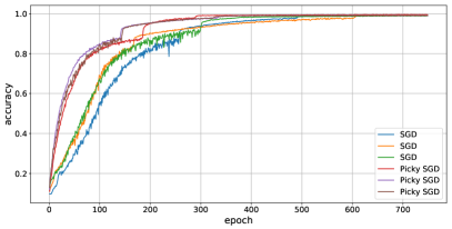
Figure 3: Training accuracy trajectory of top three configurations of Picky SGD and SGD for the four delay schedules of Fig. 2, respectively. Picky SGD is seen to perform better and more robustly than SGD across different hyperparameter configurations.

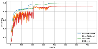
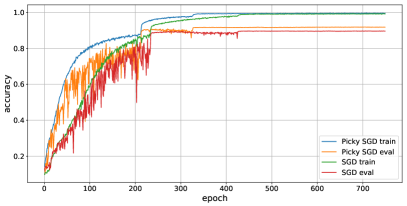
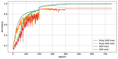
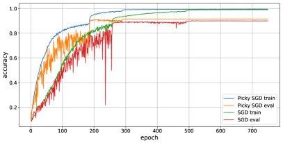
Figure 4: Train and test accuracy trajectories of Picky SGD and SGD for the four delay schedules of Fig. 2, respectively. Picky SGD is seen to outperform SGD in terms of the final test accuracy and the time it takes to achieve it, in all four scenarios.

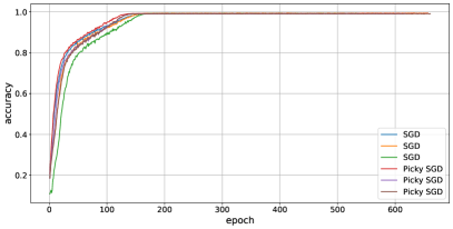
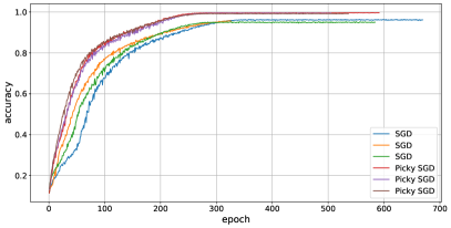
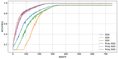
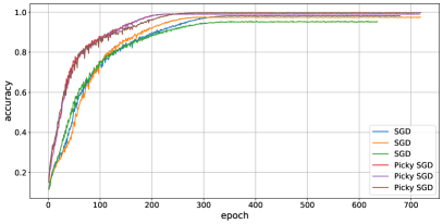
Figure 5: Train accuracy of the top three hyper-parameter configurations for the four delay schedules when trained using cosine-decay learning rate schedule. Picky SGD is again seen to significantly outperform SGD in terms of the final accuracy and the time it takes to achieve it.

Appendix C Efficient implementation of Picky SGD

In this section, we present the implementation of Picky SGD under a typical multi-worker parameter-server setting. In this setting, the state of the model is stored on a dedicated server called the parameter server, while the gradient computation is performed on a set of worker machines. At each iteration, the worker queries the parameter server for its current state, computes the gradient then sends the update to the back to server. This architecture allows an efficient use of asymmetrical and computational resources and machines under varying work loads, such as the ones commonly available in large-scale cloud platforms. Note that these systems are particularly amenable to large variations in the computational time of the gradient.

Under the setting described above, the straightforward implementations of Picky SGD are inefficient, where either the parameter server is required to keep a large portion of the history of the computation (if line 4 of the algorithm is executed by the parameter server) or the workers need to query the parameter server twice during each gradient computation (in case the line 4 is executed by the workers).

The overhead described above can be eliminated by executing line 4 at the worker side and observing that after sending the appropriate update to the parameter server, the worker has all the information it needs in order to compute the next iterate without an additional query to the parameter server. See Algorithm 6 for a pseudo-code describing the worker side of the proposed method (the parameter server implementation proceeds simply by receiving the gradient and updating the parameter state accordingly).

Algorithm 6 Picky SGD: worker implementation

1:  input: learning rate $\eta$, target accuracy $\epsilon$.

2:  query parameter server $\rightarrow x$.

3:  loop

4:     compute stochastic gradient $g$ such that $\mathbb{E}[g]=\nabla f(x)$.

5:     query parameter server $\rightarrow x^{\prime}$.

6:     if $\norm{x-x^{\prime}}\leq\ifrac{\epsilon}{(2\beta)}$ then

7:        send update to parameter server $\leftarrow g$.

8:        set: $x\leftarrow x^{\prime}-\eta g$.

9:     else

10:        set: $x\leftarrow x^{\prime}$.

11:     end if

12:  end loop

Finally, regarding the tuning of the threshold parameter $\ifrac{\epsilon}{(2\beta)}$, a simple strategy of selecting a good threshold we found to be effective in practice, is to log all distances $\|x-x^{\prime}\|$ that occur during a typical execution and taking 99th percentile of these distances as the threshold. This ensures robustness to long delays while maintaining near-optimal performance.

References

• Abadi et al. (2015) Martín Abadi, Ashish Agarwal, Paul Barham, Eugene Brevdo, Zhifeng Chen, Craig Citro, Greg S. Corrado, Andy Davis, Jeffrey Dean, Matthieu Devin, Sanjay Ghemawat, Ian Goodfellow, Andrew Harp, Geoffrey Irving, Michael Isard, Yangqing Jia, Rafal Jozefowicz, Lukasz Kaiser, Manjunath Kudlur, Josh Levenberg, Dandelion Mané, Rajat Monga, Sherry Moore, Derek Murray, Chris Olah, Mike Schuster, Jonathon Shlens, Benoit Steiner, Ilya Sutskever, Kunal Talwar, Paul Tucker, Vincent Vanhoucke, Vijay Vasudevan, Fernanda Viégas, Oriol Vinyals, Pete Warden, Martin Wattenberg, Martin Wicke, Yuan Yu, and Xiaoqiang Zheng. TensorFlow: Large-scale machine learning on heterogeneous systems, 2015. URL https://www.tensorflow.org/. Software available from tensorflow.org.
• Agarwal and Duchi (2012) Alekh Agarwal and John C Duchi. Distributed delayed stochastic optimization. In 2012 IEEE 51st IEEE Conference on Decision and Control (CDC), pages 5451–5452. IEEE, 2012.
• Alistarh et al. (2017) Dan Alistarh, Demjan Grubic, Jerry Z Li, Ryota Tomioka, and Milan Vojnovic. Qsgd: communication-efficient sgd via gradient quantization and encoding. In Proceedings of the 31st International Conference on Neural Information Processing Systems, pages 1707–1718, 2017.
• Arjevani et al. (2020) Yossi Arjevani, Ohad Shamir, and Nathan Srebro. A tight convergence analysis for stochastic gradient descent with delayed updates. In Algorithmic Learning Theory, pages 111–132. PMLR, 2020.
• Aviv et al. (2021) Rotem Zamir Aviv, Ido Hakimi, Assaf Schuster, and Kfir Yehuda Levy. Asynchronous distributed learning : Adapting to gradient delays without prior knowledge. In Marina Meila and Tong Zhang, editors, Proceedings of the 38th International Conference on Machine Learning, volume 139 of Proceedings of Machine Learning Research, pages 436–445. PMLR, 18–24 Jul 2021. URL https://proceedings.mlr.press/v139/aviv21a.html.
• Bertsekas and Tsitsiklis (1997) D.P. Bertsekas and J.N. Tsitsiklis. Parallel and Distributed Computation: Numerical Methods. Athena Scientific, 1997.
• Chaturapruek et al. (2015) Sorathan Chaturapruek, John C Duchi, and Christopher Ré. Asynchronous stochastic convex optimization: the noise is in the noise and sgd don’t care. Advances in Neural Information Processing Systems, 28:1531–1539, 2015.
• Cotter et al. (2011) Andrew Cotter, Ohad Shamir, Nathan Srebro, and Karthik Sridharan. Better mini-batch algorithms via accelerated gradient methods. In Proceedings of the 24th International Conference on Neural Information Processing Systems, pages 1647–1655, 2011.
• Dekel et al. (2012) Ofer Dekel, Ran Gilad-Bachrach, Ohad Shamir, and Lin Xiao. Optimal distributed online prediction using mini-batches. Journal of Machine Learning Research, 13(1), 2012.
• Duchi et al. (2012) John C Duchi, Peter L Bartlett, and Martin J Wainwright. Randomized smoothing for stochastic optimization. SIAM Journal on Optimization, 22(2):674–701, 2012.
• Feyzmahdavian et al. (2016) Hamid Reza Feyzmahdavian, Arda Aytekin, and Mikael Johansson. An asynchronous mini-batch algorithm for regularized stochastic optimization. IEEE Transactions on Automatic Control, 61(12):3740–3754, 2016.
• Ghadimi and Lan (2013) Saeed Ghadimi and Guanghui Lan. Stochastic first-and zeroth-order methods for nonconvex stochastic programming. SIAM Journal on Optimization, 23(4):2341–2368, 2013.
• He et al. (2016) Kaiming He, Xiangyu Zhang, Shaoqing Ren, and Jian Sun. Deep residual learning for image recognition. In Proceedings of the IEEE conference on computer vision and pattern recognition, pages 770–778, 2016.
• Karimireddy et al. (2019) Sai Praneeth Karimireddy, Quentin Rebjock, Sebastian Stich, and Martin Jaggi. Error feedback fixes signsgd and other gradient compression schemes. In International Conference on Machine Learning, pages 3252–3261. PMLR, 2019.
• Krizhevsky (2009) A. Krizhevsky. Learning multiple layers of features from tiny images. Technical report, Computer Science Department, University of Toronto, April 2009.
• Lan (2012) Guanghui Lan. An optimal method for stochastic composite optimization. Mathematical Programming, 133(1):365–397, 2012.
• Leblond et al. (2018) Rémi Leblond, Fabian Pedregosa, and Simon Lacoste-Julien. Improved asynchronous parallel optimization analysis for stochastic incremental methods. Journal of Machine Learning Research, 19:1–68, 2018.
• Lian et al. (2015) Xiangru Lian, Yijun Huang, Yuncheng Li, and Ji Liu. Asynchronous parallel stochastic gradient for nonconvex optimization. In Proceedings of the 28th International Conference on Neural Information Processing Systems-Volume 2, pages 2737–2745, 2015.
• Mania et al. (2017) Horia Mania, Xinghao Pan, Dimitris Papailiopoulos, Benjamin Recht, Kannan Ramchandran, and Michael I Jordan. Perturbed iterate analysis for asynchronous stochastic optimization. SIAM Journal on Optimization, 27(4):2202–2229, 2017.
• McMahan et al. (2017) Brendan McMahan, Eider Moore, Daniel Ramage, Seth Hampson, and Blaise Aguera y Arcas. Communication-efficient learning of deep networks from decentralized data. In Artificial Intelligence and Statistics, pages 1273–1282. PMLR, 2017.
• Nedić et al. (2001) Angelia Nedić, Dimitri P Bertsekas, and Vivek S Borkar. Distributed asynchronous incremental subgradient methods. Studies in Computational Mathematics, 8(C):381–407, 2001.
• Nesterov (2003) Yurii Nesterov. Introductory lectures on convex optimization: A basic course, volume 87. Springer Science & Business Media, 2003.
• Nesterov et al. (2018) Yurii Nesterov et al. Lectures on convex optimization, volume 137. Springer, 2018.
• Niu et al. (2011) Feng Niu, Benjamin Recht, Christopher Re, and Stephen J Wright. Hogwild! a lock-free approach to parallelizing stochastic gradient descent. In Proceedings of the 24th International Conference on Neural Information Processing Systems, pages 693–701, 2011.
• Reddi et al. (2015) Sashank J Reddi, Ahmed Hefny, Suvrit Sra, Barnabás Pöczos, and Alex Smola. On variance reduction in stochastic gradient descent and its asynchronous variants. In Proceedings of the 28th International Conference on Neural Information Processing Systems-Volume 2, pages 2647–2655, 2015.
• Stich and Karimireddy (2020) Sebastian U Stich and Sai Praneeth Karimireddy. The error-feedback framework: Better rates for sgd with delayed gradients and compressed updates. Journal of Machine Learning Research, 21:1–36, 2020.
• Woodworth et al. (2020) Blake Woodworth, Kumar Kshitij Patel, Sebastian Stich, Zhen Dai, Brian Bullins, Brendan Mcmahan, Ohad Shamir, and Nathan Srebro. Is local sgd better than minibatch sgd? In International Conference on Machine Learning, pages 10334–10343. PMLR, 2020.
• Zhou et al. (2018) Kaiwen Zhou, Fanhua Shang, and James Cheng. A simple stochastic variance reduced algorithm with fast convergence rates. In International Conference on Machine Learning, pages 5980–5989. PMLR, 2018.