Multiple Organ Failure Prediction with Classifier-Guided Generative Adversarial Imputation Networks

Abstract.

Multiple organ failure (MOF) is a severe syndrome with a high mortality rate among Intensive Care Unit (ICU) patients. Early and precise detection is critical for clinicians to make timely decisions. An essential challenge in applying machine learning models to electronic health records (EHRs) is the pervasiveness of missing values. Most existing imputation methods are involved in the data preprocessing phase, failing to capture the relationship between data and outcome for downstream predictions. In this paper, we propose classifier-guided generative adversarial imputation networks (Classifier-GAIN) for MOF prediction to bridge this gap, by incorporating both observed data and label information. Specifically, the classifier takes imputed values from the generator(imputer) to predict task outcomes and provides additional supervision signals to the generator by joint training. The classifier-guide generator imputes missing values with label-awareness during training, improving the classifier’s performance during inference. We conduct extensive experiments showing that our approach consistently outperforms classical and state-of-art neural baselines across a range of missing data scenarios and evaluation metrics.

1. Introduction

Multiple organ failure (MOF) is a life-threatening syndrome with variable causes, including sepsis (Rossaint and Zarbock, 2015), pathogens (Harjola et al., 2017), and complicated pathogenesis (Wang et al., 2018). It is a major cause of death in the surgical intensive care unit (ICU) (Durham et al., 2003). Care in the first few hours after admission is critical to patient outcomes. This period is also more prone to medical decision errors in ICUs than later times (Otero-López et al., 2006). Thus, an effective and real-time prediction is essential for clinicians to provide appropriate treatment and increase the survival rates for MOF patients.

With the rapid growth of electronic health record (EHR) data availability, machine learning models have drawn increasing attention for MOF prediction. Missing values are a pervasive and serious medical data issue, which could be caused by various reasons such as lost records or inability to collect the data during some time periods  (Zhang et al., 2016). There exist many imputation algorithms, such as mean value imputation (Acuna and Rodriguez, 2004), multivariate imputation by chained equations (MICE) (Buuren and Groothuis-Oudshoorn, 2010) and generative adversarial imputation nets (GAIN) (Yoon et al., 2018) which impute missing components by adapting generative adversarial networks (GANs). However, these methods focus only on constructing the distribution between the unobserved components and the observed ones, without considering the underlying connections with specific downstream tasks, as is shown in the Figure 1.

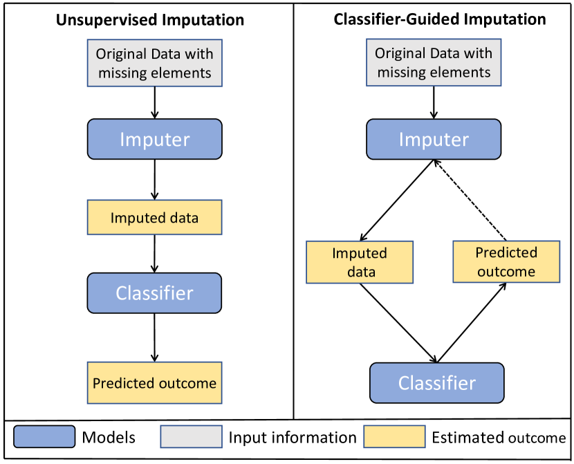
Figure 1. Workflow comparison of unsupervised imputers (left) and Classifier-GAIN (right). Classifier-guided imputers learn from the classifier during training and improve classification during inference, while unsupervised imputers learn only from the partially observed data in the data-prepossessing phase. The solid lines represent processes that occur during both the training and inference phase, while the dashed line represents the step that only occurs during training. Note that our final goal is to improve the classifier’s performance utilizing imputed data.

Recently, GANs (Goodfellow et al., 2014) have made significant progress on data generation. Labels can be incorporated in the GAN framework, e.g. CGAN (Mirza and Osindero, 2014) and AC-GAN (Odena et al., 2017), to generate label-aware outputs. Semi-supervised GAN  (Odena, 2016) introduces a classifying discriminator to output either the validity of data or its class. Triple-GAN  (Li et al., 2017) is further proposed by adding an additional classifier to separate the role of the discriminator in Semi-supervised GAN. These works leverage label information to improve data generation and their generators have to take ground truth labels to generate label-aware data, which is not applicable in classification problems during inference.

In this paper, we propose a classifier-guided missing value imputation framework for MOF prediction with early-stage measurements after admission. The generator uses observed data and random noise to impute missing components and obtains imputed data; the classifier takes the generator’s outcomes, models the relationship between imputed data and labels by joint training with the generator, and outputs estimated labels. The discriminator attempts to identify which component is observed by taking imputed data from the generator and predicted label information from the classifier.

The key contributions of this paper include:

1) We propose a classifier-guided missing value imputation deep learning framework for MOF prediction, which incorporates both observed data and label for modeling label-aware imputation during training to help classification during inference. To the best of our knowledge, this is the first GAN-based end-to-end deep learning architecture for MOF prediction with missing values.

2) Experimental results on both synthetic and real-world MOF datasets show that our Classifier-GAIN outperforms GAIN and MICE consistently in different missing ratio scenarios and evaluation metrics.

3) Visualization of the values imputed by our approach further validates the effectiveness of Classifier-GAIN compared to various baselines.

The remainder of our paper is organized as follows. Preliminaries are introduced in Section 2, followed by the details of our proposed approach in Section 3. Experimental results are reported in Section 4. In Section 5, we review the existing related work, and conclusions are given in Section 6.

2. Preliminaries

We formulate the MOF prediction as a binary classification problem with missing components in multiple features. In this section, we describe the problem definition in Section 2.1 and review the GAIN imputation algorithm in Section 2.2. The related notations are summarized in Table 1. Specifically, throughout this paper, we utilize lower-case letters, e.g. x, to denote the data vector. $p(\textbf{x})$ is the probability distribution function of x. 1 denotes a d-dimensional vector of $1$s, and letters with hats such as $\hat{\textbf{x}}$ denote estimated vectors.

Table 1. Notation definitions

Notations	Description
$i$	index of observations
$j$	index of observed features
$d\in\mathbb{N}$	number of observed features
$N\in\mathbb{N}$	total number of observations
$n\in\mathbb{N}$	size of minibatch
x	data vector
$y$	outcome indicator
m	mask vector
z	noise vector
h	hint vector
b	binary vector for calculating hint
$\tilde{\textbf{x}}$	combination of partially observed data and NAs
$\ddot{\textbf{x}}$	combination of partially observed data and noise
$G$	generator
$C$	classifier
$D$	discriminator
g	reconstructed vector, the output of G
$\hat{\textbf{x}}$	imputed data vector
$\hat{\textbf{m}}$	estimated mask, the output of D
$\hat{y}$	estimated label, the output of C

2.1. Problem definition

Let $\mathcal{X}^{d}$ be a $d$-dimensional space and x a data vector, taking values in $\mathcal{X}^{d}$ following distribution $p(\textbf{x})$. We denote $x_{j}$ as the $j$-th feature in x. Binary mask vector $\textbf{m}\in\{0,1\}^{d}$ indicates if the corresponding element in x is missing or not, where $x_{j}$ is observed if $m_{j}=1$, otherwise $x_{j}$ is missing. To clarify the observed and missing components, we define a new vector $\tilde{\textbf{x}}=(\tilde{x}_{1},\cdots,\tilde{x}_{d})$ as follows:

$$\tilde{x}_{j\in\{1,2,...,d\}}=\begin{cases}x_{j},&\text{if }m_{j}=1,\\ \textit{NA},&\text{if }m_{j}=0.\end{cases}$$

Supposing that $y\in\{0,1\}$ is the binary outcome indicator for each sample, we can represent the dataset as a collection of $N$ i.i.d. samples $\{(\tilde{\textbf{x}}_{i},\textbf{m}_{i}),y_{i}\}_{i=1}^{N}$.

We aim to impute the missing components in every $\tilde{\textbf{x}}$, and predict the outcome $y$ for all samples by leveraging the imputed data vector. Formally, we seek to model $p(y|\tilde{\textbf{x}})$: the conditional distribution of the task outcome given a partially observed data vector.

2.2. Generative adversarial imputation networks (GAIN)

GAIN (Yoon et al., 2018) was proposed to impute missing components with a GAN framework. In GAIN, the generator takes the observed components in $\tilde{\textbf{x}}$, mask vector m and a noise vector z as inputs, and outputs a completed data vector. The discriminator tries to distinguish the observed components and the missing ones. Furthermore, a hint vector h is introduced to provide additional missing information for alleviating the diversity of the imputation result.

The generator, G, takes

$$\ddot{\textbf{x}}=\textbf{m}\odot\tilde{\textbf{x}}+(\textbf{1}-\textbf{m})\odot\textbf{z},$$

a combination of $\tilde{\textbf{x}}$ and z by element-wise multiplication with m, as input, and outputs g, the reconstructed vector,

$$\textbf{g}=G(\ddot{\textbf{x}}).$$

Note that g is an output vector for every component, even if values are not missing in the data vector.

Thus, another element-wise multiplication is performed to calculate the imputed data vector via

$$\hat{\textbf{x}}=\textbf{m}\odot\tilde{\textbf{x}}+(\textbf{1}-\textbf{m})\odot\textbf{g},$$

where $\hat{\textbf{x}}$ is obtained by taking the observed part in $\tilde{\textbf{x}}$ and replacing each NA by the corresponding value in g.

The discriminator serves as an adversarial character to train G by taking in the imputed data vector $\hat{\textbf{x}}$ and the hint vector h, following the distribution $p(\textbf{h}|\textbf{m})$. The output of the discriminator is a distribution to identify which components in $\hat{\textbf{x}}$ are observed. To help the discriminator distinguish imputations and observations, h provides certain information about m and its amount can be controlled by adjusting h in different settings. Specifically, a binary random variable $\textbf{b}\in\{0,1\}^{d}$ is randomly drawn with $P(b_{j}=1)=p$. Then, $\textbf{h}|\textbf{m}$ is calculated by

$$\textbf{h}=\textbf{m}\odot\textbf{b}+0.5(\textbf{1}-\textbf{b}),$$

such that the discriminator will get mask information by $h_{j}=m_{j}$ if $b_{j}=1$, otherwise, no information provided.

3. Methodology

Notably, conditional information such as labels can improve the performance of the generator (Mirza and Osindero, 2014; Odena et al., 2017), and the completed data vector can enhance its task prediction result. However, state-of-art imputation methods, e.g. GAIN, do not make use of the relationship between observations and outcome labels, which could provide additional information to help downstream classification tasks. Therefore, we propose Classifier-GAIN to bridge this gap. Figure 2 depicts the overall architecture. We explain each of the components and the training process of Classifier-GAIN in detail in Section 3.1$\sim$ 3.2.

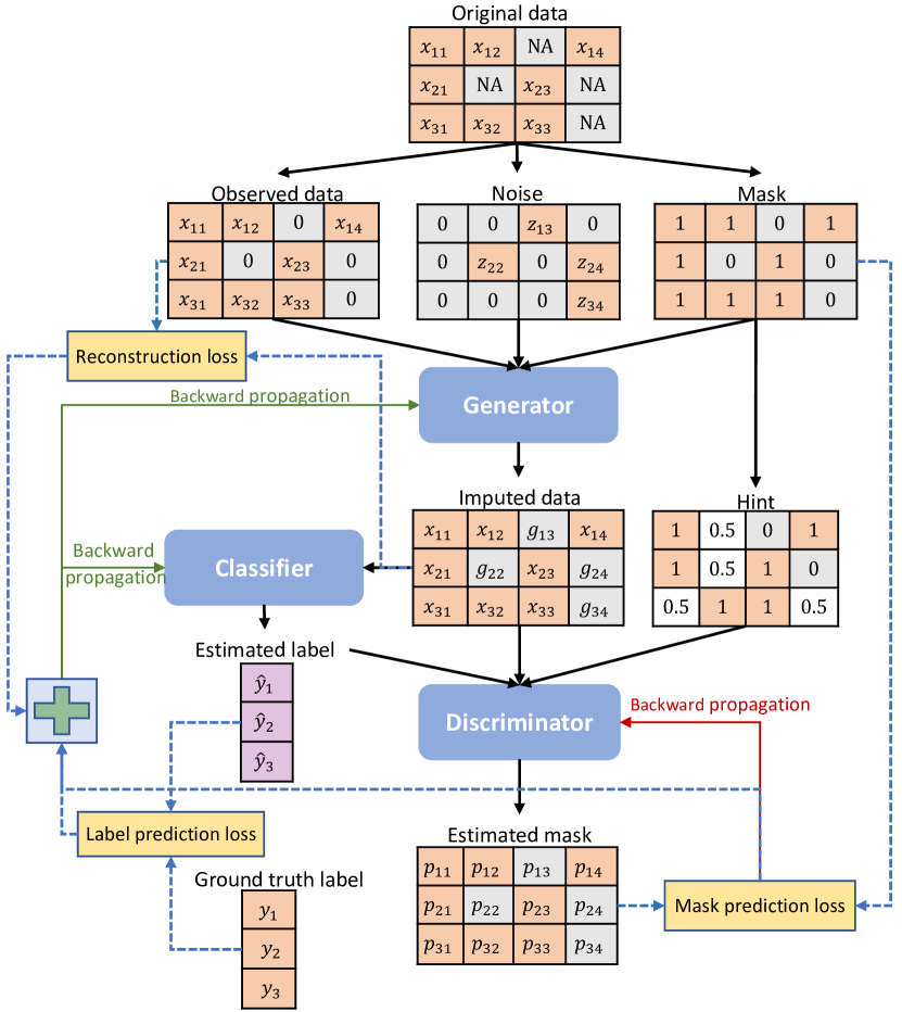
Figure 2. The overall architecture of Classifier-GAIN with three samples (adapted from GAIN (Yoon et al., 2018)). Each row in the matrices and vectors corresponds to a sample. The input of our network is the original data vector with missing components. The generator takes partial observation data, a noise matrix filling missing components and mask, and outputs imputed data, which is then fed into the classifier to obtain the estimated labels. The imputed data and the estimated labels along with a hint matrix are fed into the discriminator to estimate the mask. Dashed lines represent information flows for loss calculation. Green solid lines represent backward propagation for the generator and the classifier training, and the red solid line represents the backward propagation for the discriminator training.

3.1. Classifier-guided generative adversarial imputation nets

In an imputation setting, we propose to fill in the missing components NAs in $\tilde{\textbf{x}}$, using the distribution of data obtained by the generator, G. To guide the data imputation and predict the final task outcome, the classifier, C, takes imputed data and is trained together with G. The discriminator D plays an adversarial role to train G, with additional label prediction information from C.

Generator and Classifier

Similar to the structure of GAIN, G takes $\tilde{\textbf{x}}$ as input and outputs $\hat{\textbf{x}}$, trying to model $p(\textbf{x}|\tilde{\textbf{x}})$, the conditional distribution of a data vector given the partial observations. The classifier C is a supervised learning model to predict the task outcome, $\hat{y}$, by taking $\hat{\textbf{x}}$ from G, which obtains the conditional distribution $P(y|\textbf{x})=P(y|\hat{\textbf{x}})$. We define the estimated outcome $\hat{y}$ by

$$\hat{y}=C(\hat{\textbf{x}}).$$

Then G and C are jointly trained to obtain the distribution $p(y,\textbf{x}|\tilde{\textbf{x}})$, making G label-aware during imputation, which is ignored by GAIN.

Discriminator

In our architecture, the discriminator D serves as an adversarial character to train G by receiving the predicted label information from C. We input $\hat{\textbf{x}}$, $\hat{y}$ and h into D to obtain the probability that each component in $\hat{\textbf{x}}$ is observed. Here, $\hat{\textbf{x}}$ and $\hat{y}$ jointly provide information to enhance D by learning the relationship between data and task outcomes, which can further strengthen G and C. We define the estimated mask variable, $\hat{\textbf{m}}\in[0,1]^{d}$, by

$$\hat{\textbf{m}}=D(\hat{\textbf{x}},\hat{y},\textbf{h}),$$

with the $j$-th item in $\hat{\textbf{m}}$ corresponding to the probability that the $j$-th item in $\hat{\textbf{x}}$ is not NA in $\tilde{\textbf{x}}$.

3.2. Classifier-GAIN training

G, C and D are trained as a min-max game by

(1) $$\min_{G,C}\max_{D}V(G,C,D)=\mathbb{E}_{\ddot{\textbf{x}},\textbf{m},\textbf{h}}\Bigg{[}\textbf{m}\log\Big{(}D\big{(}G(\ddot{\textbf{x}}),C(G(\ddot{\textbf{x}})),\textbf{h}\big{)}\Big{)}\\ +(\textbf{1}-\textbf{m})\log\Big{(}\textbf{1}-D\big{(}G(\ddot{\textbf{x}}),C(G(\ddot{\textbf{x}})),\textbf{h}\big{)}\Big{)}\Bigg{]},$$

where $\log$ is an element-wise logarithm. Specifically, We train G and C together to minimize the probability of D identifying m, maximize the probability of correctly predicting $y$ and minimize the reconstruction loss of observed components. We train D to maximize the probability of correctly predicting m.

On each iteration, G and C are updated $k$ times with objective function, $\mathcal{L}_{C\&G}$, which is a weighted sum of three losses

(2) $$\mathcal{L}_{C\&G}=\mathcal{L}_{G}(\textbf{m},\hat{\textbf{m}})+\alpha\mathcal{L}_{R}(\textbf{x},\hat{\textbf{x}})+\beta\mathcal{L}_{C}(y,\hat{y}),$$

where $\alpha$ and $\beta$ are hyper-parameters.

The first loss, $\mathcal{L}_{G}$, is an adversarial loss, which applies to missing components ($m_{j}=0$) by

(3) $$\mathcal{L}_{G}(\textbf{m},\hat{\textbf{m}})=-\sum_{j=1}^{d}\Big{[}(1-m_{j})\log(\hat{m}_{j})\Big{]}.$$

The second loss, $\mathcal{L}_{R}$, is a reconstruction loss, which applies to observed components ($m_{j}=1$) by

(4) $$\mathcal{L}_{R}(\textbf{x},\hat{\textbf{x}})=\sum_{j=1}^{d}m_{j}L_{R}(x_{j},\hat{x}_{j}),$$

where

$$L_{R}(x_{j},\hat{x}_{j})=\begin{cases}(x_{j}-\hat{x}_{j})^{2},&\text{for numerical variables,}\\ -x_{j}\log(\hat{x}_{j}),&\text{for binary variables. }\end{cases}$$

The third loss, $\mathcal{L}_{C}$, is a binary cross entropy loss for task prediction given by

(5) $$\mathcal{L}_{C}(y,\hat{y})=-\big{[}y\log{(\hat{y})}+(1-y)\log(1-\hat{y})\big{]}.$$

Note that as G and C are updated together via Eq. 2, C ’s performance will influence G’s parameters to guide the missing component imputation.

D updates once at each iteration with objective function

(6) $$\mathcal{L}_{D}(\textbf{m},\hat{\textbf{m}})=-\sum_{j=1}^{d}\Big{[}m_{j}\log(\hat{m}_{j})+(1-m_{j})\log(1-\hat{m}_{j})\Big{]}.$$

The detailed training process is shown in Algorithm 1.

Algorithm 1 Minibatch Classifier-GAIN training

1:Input: Original data vector with missing component $\tilde{\textbf{x}}$, mask vector m, ground truth label $y$, the probability for drawing the hint vector p. hyper-parameters $\alpha$ and $\beta$.

2:repeat

3:     Generator and Classifier

4:     Sample a batch of n binary vector $\{\textbf{b}_{i}\}_{i=1}^{n}\sim\text{Bern}(p)^{d}$

5:     for k steps do

6:         Sample a batch of n noises $\{\textbf{z}_{i}\}_{i=1}^{n}\sim U(0,1]^{d}$

7:         for $i\leftarrow 1\text{ to }n$ do

8:              $\textbf{h}_{i}\leftarrow\textbf{m}_{i}\odot\textbf{b}_{i}+0.5(\textbf{1}-\textbf{b}_{i})$

9:              $\ddot{\textbf{x}}_{i}\leftarrow\textbf{m}_{i}\odot\tilde{\textbf{x}}_{i}+(\textbf{1}-\textbf{m}_{i})\odot\textbf{z}_{i}$

10:              Imputed data $\textbf{g}_{i}\leftarrow G(\ddot{\textbf{x}}_{i})$

11:              $\hat{\textbf{x}}_{i}\leftarrow\textbf{m}_{i}\odot\tilde{\textbf{x}}_{i}+(\textbf{1}-\textbf{m}_{i})\odot\textbf{g}_{i}$

12:              Obtain $\hat{y}_{i}\leftarrow C(\hat{\textbf{x}}_{i})$

13:              Obtain $\hat{\textbf{m}}_{i}\leftarrow D(\hat{\textbf{x}}_{i},\hat{y}_{i},\textbf{h}_{i})$

14:         end for

15:         Update generator $G$ and classifier $C$ together via stochastic gradient descent (SGD):

16:         $\bigtriangledown_{G}~{}\frac{1}{n}\sum_{i=1}^{n}\mathcal{L}_{G}(\textbf{m}_{i},\hat{\textbf{m}}_{i})+\alpha\mathcal{L}_{R}(\textbf{x}_{i},\hat{\textbf{x}}_{i})+\beta\mathcal{L}_{C}(y_{i},\hat{y}_{i})$

17:     end for

18:     

19:     Discriminator

20:     Sample a batch of n binary vector $\{\textbf{b}_{i}\}_{i=1}^{n}\sim\text{Bern}(p)^{d}$

21:     for $i\leftarrow 1\text{ to }n$ do

22:         $\textbf{h}_{i}\leftarrow\textbf{m}_{i}\odot\textbf{b}_{i}+0.5(\textbf{1}-\textbf{b}_{i})$

23:         Obtain $\hat{\textbf{m}}_{i}\leftarrow D(\hat{\textbf{x}}_{i},\hat{y}_{i},\textbf{h}_{i})$

24:     end for

25:     Update discriminator with fixed G and C via SGD

26:     $\bigtriangledown_{D}~{}\frac{1}{n}\sum_{i=1}^{n}\mathcal{L}_{D}(\textbf{m}_{i},\hat{\textbf{m}}_{i})$

27:until Classifier-GAIN converges

4. Experiments

In this section, we conduct experiments on two datasets: the PhysioNet sepsis synthetic dataset and the UCSF real-world EHR dataset, introduced in Section 4.1, to evaluate Classifier-GAIN’s performance. Particularly, we investigate

1. Does the classifier-guided imputation help the downstream MOF prediction?

2. How does the proposed algorithm perform across different missing ratio scenarios?

We explain the experimental settings in Section 4.2. The performance comparisons of Classifier-GAIN against other imputation algorithms for MOF prediction are shown in Section 4.3, followed by the visualizations of the imputed missing values of the UCSF MOF dataset in Section  4.4.

4.1. Dataset

For the PhysioNet sepsis dataset, 10,587 patients and 40 features are contained. We randomly select $80\%$ of the instances as the training set, $10\%$ as the development set, and $10\%$ as the testing set. For the UCSF MOF dataset, 2,160 patients and 29 features are contained. we perform a 5-fold cross validation, considering the dataset’s size and models’ training time. The detailed description of datasets as follows:

PhysioNet sepsis synthetic dataset

Sepsis is a severe critical illness syndrome that can result in MOF (Rossaint and Zarbock, 2015). Since MOF is the fatal end of sepsis progression(Bravo-Merodio et al., 2019), early detection of sepsis and antibiotic prescription are critical for improving MOF patient outcomes. We built a synthetic dataset based on the physiological data (Reyna et al., 2019) provided by PhysioNet, sourced from ICU patients. Each patient contains $40$ hourly measurements in three categories (vital signs, laboratory values and demographics) and the sepsis outcome in each hour. To obtain the sepsis outcome in the early stages, we focus on the first 6 hours’ records of each feature. We take the first-appearance measurement of each feature in the first six hours after admission. If the value of a feature was not recorded in the first six hours, we assume that value was missing. We exclude the patients whose features were entirely missing in the first six hours. We label a patient with sepsis as 1, otherwise as 0. To obtain a completed synthetic dataset for further experiments, we apply KNN (with $K=5$) to impute the original missing components and SMOTE to balance the data. After data preprocessing, we obtained 10,587 patients, among which 5,808 patients are with sepsis and 4,779 without sepsis.

UCSF MOF real-world dataset

Our UCSF MOF dataset, collected from the UCSF/San Francisco General Hospital and Trauma Center, contains 2,190 patients admitted to a Level I trauma center. Both demographic information, such as gender, age, BMI (body mass index), and injury measurements, e.g. injury severity score (ISS), traumatic brain injury, and Glasgow Coma Scale (GCS), were measured at the admission time of each patient. Laboratory results (D-Dimer, creatinine, white blood cell etc.) and physical vital signs (for example heart rate, respiratory rate, systolic blood pressure etc.) were recorded at different hours. Unique ICU treatments such as blood transfusion units, fresh frozen plasma transfusion and crystalloids for fluid resuscitation were slotted into time intervals such as 0 to 24 hours. Medical treatments (vasopressor, Heparin and Factor VII et al.) were reported daily after admission.

To analyze the MOF states associated with patients’ early-stage status, we select either the first day or the initial hour records manually. We extract features with importance scores higher than 2% using forests of trees in Scikit-learn (Pedregosa et al., 2011), and remove the patients whose data were utterly missing in the early stage or whose MOF outcome was not recorded. After data preprocessing and removal of abnormal values, we are left with 2,160 patients and 29 measurements. Selected features are categorized by types, and detailed statistics are shown in Appendix A. Two blood test features, D-Dimer and Factor VII, had a missing rate higher than $40\%$. The body mass index (BMI) missed $17.4\%$. Factor VII treatment, partial thromboplastin time (PTT), respiratory rate and systolic blood pressure were missing at rates between $5\%$ and $10\%$. The remainder of the features were missing at rates less than $5\%$. The rate of missing data for each feature is listed in Table 2, ordered from high to low. Missing values account for $6.42\%$ among all observations and the labelling ratio between No MOF (class 0) and MOF (class 1) is $11:1$ in the dataset.

Table 2. Rates of missing data in the UCSF dataset

Missing rate	Feature
41.9$\%$	D-Dimer
41.6$\%$	Factor VII (blood test)
17.4$\%$	BMI
$10\%\geq\&>5\%$	Factor VII treatment, PTT, Respiratory, SBP
$5\%\geq\&>0\%$	HR, numribfxs, GCS, Vasopressor, Bun, Serumco2,
	PLTs, Crystalloids, Crystalloids, WBC, HGB, HCT,
	AIS scores, FFP_units, Blood_units, age, iss,
	Thromboembolic complication, Heparin_gtt
$0\%$	Gender

4.2. Experimental settings

Evaluation metrics

We measure the performance of Classifier-GAIN and baselines by both macro F1-score and area under the ROC curve (AUC-ROC).

Macro F1-score is defined as the mean of class-wise F1 scores which assigns equal importance to every class. It is low for models that perform well on the common classes, while performing poorly on the rare classes. For the Macro F1-Score calculation, we use 0.5 as the predicted value threshold.

AUC-ROC is also commonly used for MOF prediction (Bakker et al., 1996; Papachristou et al., 2010). AUC-ROC assesses the overall preference of a classifier by summarizing over all possible classification thresholds. In binary classification problems, the higher the AUC-ROC, the better the model’s performance in identifying the two classes.

Table 3. Hidden layer setting of different modules in UCSF and Sepsis datasets.

Dataset	Network	Hidden layer 1	Hidden layer 2	Dropout rate
UCSF	Classifier	32	16	0.1
	Generator	64	32	0.1
	Discriminator	64	32	0.1
Sepsis	Classifier	128	64	0.1
	Generator	64	32	0.1
	Discriminator	64	32	0.1

Missing Rate	macro F1-score				AUC-ROC
	Classifier-GAIN	Simple imputation	MICE	GAIN	Classifier-GAIN	Simple imputation	MICE	GAIN
$0\%$	Upper bound: $84.8\pm 0.1$				Upper bound: $90.9\pm 0.3$
$20\%$	83.2 $\pm$ 0.3	67.8 $\pm$ 2.1	68.6 $\pm$ 1.5	69.5 $\pm$ 1.8	88.3 $\pm$ 0.6	83.1 $\pm$ 0.9	84.3 $\pm$ 1.5	83.4 $\pm$ 1.4
$25\%$	82.9 $\pm$ 0.2	68.3 $\pm$ 3.3	66.9 $\pm$ 1.5	65.9 $\pm$ 1.6	87.1 $\pm$ 0.4	81.8 $\pm$ 1.2	81.9 $\pm$ 0.6	81.3 $\pm$ 0.6
$30\%$	80.8 $\pm$ 0.8	67.4 $\pm$ 2.1	67.3 $\pm$ 1.1	67.1 $\pm$ 2.0	86.4 $\pm$ 0.6	81.9 $\pm$ 1.0	81.0 $\pm$ 0.9	81.8 $\pm$ 1.0
$35\%$	79.7 $\pm$ 0.9	66.9 $\pm$ 1.6	68.9 $\pm$ 1.5	66.2 $\pm$ 3.3	84.8 $\pm$ 0.4	81.2 $\pm$ 1.1	80.3 $\pm$ 1.0	81.7 $\pm$ 0.8
$40\%$	78.8 $\pm$ 0.7	64.6 $\pm$ 2.6	66.9 $\pm$ 2.3	64.8 $\pm$ 3.5	83.9 $\pm$ 0.6	80.3 $\pm$ 0.4	80.0 $\pm$ 1.1	81.2 $\pm$ 0.9
$45\%$	77.2 $\pm$ 0.5	65.6 $\pm$ 3.0	66.4 $\pm$ 1.9	65.4 $\pm$ 3.2	81.1 $\pm$ 0.4	79.5 $\pm$ 0.9	79.2 $\pm$ 0.9	79.0 $\pm$ 0.7
$50\%$	77.7 $\pm$ 0.8	65.1 $\pm$ 1.6	63.7 $\pm$ 1.0	65.5 $\pm$ 2.1	82.1 $\pm$ 0.7	80.5 $\pm$ 0.4	74.7 $\pm$ 0.6	80.7 $\pm$ 0.6

Table 4. Model performance (%) on PhysioNet sepsis dataset in different missing ratio settings.

Model configurations

We compare Classifier-GAIN with both classical and state-of-art neural baselines for MOF prediction as follows:

1. Simple imputation: It imputes missing components by mean imputation and most frequent imputation for continuous and categorical variables, respectively.

2. MICE (Buuren and Groothuis-Oudshoorn, 2010): It is a multiple imputation method, accounting for the statistical uncertainty in the imputations.

3. GAIN (Yoon et al., 2018): It is a deep learning adversarial imputation framework, which we explained in Section 2.2 in detail.

Each of methods (1), (2) and (3) is separated into two steps. First we impute missing components by the corresponding method. Then we utilize a binary classifier to predict the subjects’ outcomes by taking imputed data. For our proposed Classifier-GAIN, we take the partially observed data as input, and output both an imputed data and classification outcomes.

In order to make the performance comparison as fair as possible, we assign the same structure and hidden size for all classifiers. GAIN has exactly the same structure in the generator and the same number of hidden layers in the discriminator as Classifier-GAIN. All of the networks are designed as multi-layer perceptrons with two hidden layers. We use batch normalization to normalize the input layer by re-centering and re-scaling. ReLU activation function and dropout are applied after each hidden linear layer. All of the neural networks utilize Sigmoid activation at the last step for outputs. The hidden layer settings in all of our experiments are listed in Table 3.

We implement our model and its variants using PyTorch (Paszke et al., 2019), and use a GeForce GTX TITAN X 12 GB GPU for training, validation as well as testing. All of the neural networks are trained by using the Adam optimizer (Kingma and Ba, 2014), whose learning rates are selected by grid search from 0.0005 to 0.002.For the convergence of the MICE imputation, we apply the IterativeImputer in Scikit-learn (Pedregosa et al., 2011) with mean initial strategy, 100 maximum number of imputation rounds and 0.001 as tolerance of the stopping condition.

4.3. Performance comparison

We conduct each experiment by running 5 times with different random initializations and show the results in the format ”mean ± standard deviation” to answer Q1 and Q2. For readers’ convenience, we make the best performance bold in each of the performance tables in this section.

Synthetic data

To evaluate Classifier-GAIN’s capability to capture the relationship between clinical records (vital signs and laboratory values) and label outcome for downstream prediction, we randomly remove $20\%$, $25\%$, $30\%$, $35\%$, $40\%$, $45\%$ and $50\%$ of all components from clinical records, to simulate missingness resulting from the urgency of the clinical situation. We demonstrate the effectiveness of Classifier-GAIN against other baselines in Table 4. To understand the performance gap between different missing scenarios and the completed data, we train a binary classifier on the completed dataset, which we refer to as the upper bound. As shown in Table 4, Classifier-GAIN consistently outperforms the simple imputation, MICE and GAIN across the entire range of missing rates, for both evaluation metrics. Especially, when the missing rate is $25\%$, Classifier-GAIN improves $5.2\%$ and $14.6\%$ in AUC-ROC and macro F1-score, respectively, compared with the best baselines.

To quantitatively evaluate the performance of Classifier-GAIN, we derive two additional metrics: (1) the relative improvement rate (RIR),

(7) $$\frac{\text{Classifier-GAIN {-} best\_baseline}}{\text{best\_baseline}},$$

to demonstrate how much Classifier-GAIN improves compared to the best baseline, and (2) the relative gap reduction rate (RGRR),

(8) $$\frac{\text{Classifier-GAIN {-} best\_baseline}}{\text{Upper bound {-} best\_baseline}},$$

to measure the capability of Classifier-GAIN reducing the performance gap to the upper bound.

Missing Rate	macro F1-score				AUC-ROC
	Classifier-GAIN	Simple imputation	MICE	GAIN	Classifier-GAIN	Simple imputation	MICE	GAIN
$20\%$	68.3 $\pm$ 0.4	64.9 $\pm$ 1.6	65.2 $\pm$ 1.5	66.0 $\pm$ 0.9	88.9 $\pm$ 0.5	88.2 $\pm$ 0.6	89.1 $\pm$ 0.2	88.7 $\pm$ 0.5
$25\%$	67.9 $\pm$ 1.0	64.3 $\pm$ 0.5	61.5 $\pm$ 1.7	64.6 $\pm$ 1.7	88.5 $\pm$ 0.4	87.4 $\pm$ 0.5	88.4 $\pm$ 0.2	87.8 $\pm$ 0.3
$30\%$	70.2 $\pm$ 0.7	68.2 $\pm$ 1.3	61.6 $\pm$ 2.2	65.9 $\pm$ 1.0	89.5 $\pm$ 0.5	89.0 $\pm$ 0.2	87.7 $\pm$ 0.2	88.7 $\pm$ 0.4
$35\%$	67.7 $\pm$ 0.8	64.5 $\pm$ 1.2	60.4 $\pm$ 2.1	65.0 $\pm$ 0.4	88.5 $\pm$ 0.4	87.7 $\pm$ 0.4	87.0 $\pm$ 0.6	87.4 $\pm$ 0.5
$40\%$	65.7 $\pm$ 1.4	61.9 $\pm$ 0.8	58.1 $\pm$ 3.0	63.2 $\pm$ 1.2	87.8 $\pm$ 0.5	86.8 $\pm$ 0.4	85.3 $\pm$ 0.2	86.5 $\pm$ 0.5
$45\%$	65.7 $\pm$ 1.0	62.5 $\pm$ 1.4	57.3 $\pm$ 2.7	61.7 $\pm$ 1.7	86.8 $\pm$ 0.6	85.7 $\pm$ 0.7	84.6 $\pm$ 0.2	85.0 $\pm$ 0.7
$50\%$	65.0 $\pm$ 0.2	59.4 $\pm$ 1.6	57.3 $\pm$ 3.3	60.0 $\pm$ 1.7	83.9 $\pm$ 0.8	83.7 $\pm$ 0.5	84.2 $\pm$ 0.1	83.5 $\pm$ 1.4

Table 7. Model performance(%) on UCSF MOF dataset with different additionally simulated missing ratios.

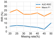
(a) The relative improvement rate ($\%$)

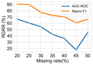
(b) The relative gap reduction rate ($\%$)

Figure 3. The relative improvement rate (left) and the relative gap reduction rate (right) of Classifier-GAIN on AUC-ROC and macro F1-score for PhysioNet sepsis dataset across different missing ratio scenarios.

The relative improvement rates calculated by Eq. 7 across different settings are shown in Figure  3 (a). For both macro F1-score and AUC-ROC, Classifier-GAIN consistently achieves a high relative improvement rate, with $21.62\%$ and $6.16\%$ on average across different scenarios, respectively. Especially, the relative improvement rate of macro F1-score is $25.80\%$ when the missing rate is $25\%$, and the relative improvement rate of AUC-ROC is $9.91\%$ when the missing rate is $50\%$. Figure  3 (b) shows the relative gap reduction rate of Classifier-GAIN with different missing ratio settings. Classifier-GAIN significantly reduces the performance gap to the upper bound, with a 75.43% relative reduction rate for macro F1-score on average compared to best baselines, making the prediction less susceptible to missingness across different scenarios. Especially when missing rates are 20% and 25% (relatively low), the relative gap reduction rates are as high as 90.58% and 89.94%, which significantly narrows the performance gap caused by missing components. Even when missing rates are 40% and 50% (very high), the relative gap reduction rates remain 60.82% and 66.35%, which further validates Classifier-GAIN’s applicability in different missing scenarios.

Real-world data

We further evaluate our model on the UCSF MOF real-world dataset, including early-stage clinical records for MOF prediction. In addition to the high missing ratio in bio-marker measurements, there is a serious label imbalance issue in this dataset, which is common in real-world clinical data. We evaluate the performance of Classifier-GAIN on the UCSF MOF dataset in the following settings: (1) imputing the original missing components and predicting MOF outcome; (2) adding additional random masks with $20\%$, $25\%$, $30\%$, $35\%$, $40\%$, $45\%$ and $50\%$ missing rates to simulate more serious missing situations in real-world data.

Table 6 reports the macro F1-score and AUC-ROC to evaluate Classifier-GAIN’s prediction performance against other methods, on the UCSF MOF dataset with original missing components (The missing ratio of features is $6.42\%$ among all patients on average.). Classifier-GAIN yields the best prediction performance as measured by both macro F1-score and AUC-ROC. All the three baselines in the original missing scenario have similar performance, and the simple imputation has the best performance in baselines, which may due to the small size and high imbalance of the real-world data. Classifier-GAIN shows better performance reflecting the classifier-guided imputation helps the downstream MOF prediction by making imputed values label-aware.

Algorithm	macro F1-score	AUC-ROC
Classifier-GAIN	71.0 $\pm$ 1.0	90.6 $\pm$ 0.5
Simple imputation	68.9 $\pm$ 1.0	90.3 $\pm$ 0.3
MICE	68.2 $\pm$ 0.8	90.0 $\pm$ 0.4
GAIN	68.2 $\pm$ 0.9	90.2 $\pm$ 0.3

Table 6. Model performance on UCSF MOF dataset with original missing components.

For more missing ratios in our simulated setting, the corresponding macro F1-score and AUC-ROC are shown in Table 7. For the macro F1-score, Classifier-GAIN consistently outperforms the best baselines more than $2\%$ across the entire range of missing rates. Especially, in the $50\%$ missing scenario, Classifier-GAIN improves $5\%$ comparing to the best baseline, GAIN. For AUC-ROC, Classifier-GAIN outperforms other post-imputation predictions in $25\%$, $30\%$, $35\%$, $40\%$, $45\%$ missing scenarios, and achieves comparable performance with MICE in $20\%$ and $50\%$ missing conditions.

4.4. Imputation results

To further visualize the imputation outcomes of the generator in Classifier-GAIN, we compare the imputation results for the original missingness in the UCSF MOF dataset of Classifier-GAIN and other baselines. We select three features: D-Dimer, Factor VII (blood test) and respiratory rate, for the imputation study. Both D-Dimer and Factor VII have more than $40\%$ missing in the original dataset, and the missing rate of respiratory rate is $7.31\%$. D-Dimer is an indicator of patients who may develop organ failure in the further course of acute pancreatitis(Radenkovic et al., 2009). Factor VII and respiratory rate are highly related to pulmonary failure (Wei, 1990; Del Sorbo and Slutsky, 2011).

Figure 4d plots the univariate distributions of selected features for MOF (MOF = 1) and no MOF (MOF = 0) patients, respectively. The blue and orange curves are density curves of observed components of features that need imputation. The blue curves represent the density curves of MOF = 0, and the orange ones represent MOF = 1. Dashed vertical lines are the imputed results of three different imputation methods: red is Classifier-GAIN, green is GAIN, and black is MICE imputation. In the UCSF MOF dataset, the feature values available with maximum density of D-Dimer, Factor VII and respiratory rate for patients who did not develop MOF are $0.86$ mg/L, $68.82\%$ and $16.92$ breaths per minute, respectively. For MOF patients, the feature values available with the maximum density are $7.71$ mg/L, $80.69\%$ and $18.75$ breaths per minute, respectively.

For panels (a) and (b), Classifier-GAIN predicts correctly for a patient without MOF, while the other classifiers, whose input data are imputed by MICE or GAIN, predict incorrectly. The imputed values of Classifier-GAIN for Factor VII and respiratory rate are relatively closer to the feature values with maximum density for no-MOF’s in both cases. Panel (c) shows a MOF patient whose data was missing the D-Dimer record. MICE and GAIN have very similar imputed value which are $3.38$ mg/L and $3.35$ mg/L, Classifier-GAIN imputes the D-Dimer as $6.53$,mg/L which follows the trend of MOF patients in this dataset. Panel (d) shows a situation that all of the classifiers predict a no-MOF case incorrectly. In this case, all three methods impute the Factor VII closer to the feature value with the maximum density for MOF’s.

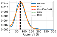
(a) Factor VII imputation for no MOF

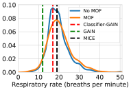
(b) Respiratory rate imputation for no MOF

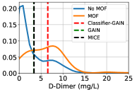
(c) D-Dimer imputation for MOF

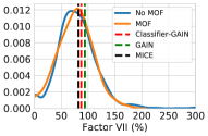
(d) Factor VII imputation for no MOF

Figure 4. Density plots of features and imputed values. The blue and orange curves are density curves of observed data points. The blue curve represents MOF = 0, and the orange represents MOF = 1. The dashed vertical lines are the imputation results of three different imputation methods.For (c), GAIN and MICE have similar imputation results, which makes lines overlap.

case.

5. related work

Generative Adversarial Networks (GAN)

GAN, introduced in (Goodfellow et al., 2014), is a game-theoretic framework for estimating the implicit distribution of data via an adversarial process. CGAN conditions the GAN framework on class labels to direct the data generation process (Mirza and Osindero, 2014). AC-GAN further improves generation performance by modifying the discriminator to contain an auxiliary decoder network (Odena et al., 2017). However, both CGAN and AC-GAN need to feed label information to their generators, which could not be achieved if the final goal is classification and the label information is unknown during inference. Semi-supervised GAN (Odena, 2016) performs GAN in a semi-supervised context to make the discriminator output either data validation or class labels. Triple-GAN facilitates the convergence of both the generator and the discriminator by introducing the ”third player” – classifier (Li et al., 2017).

Researchers have also applied GANs on missing value imputation. In GAIN (Yoon et al., 2018), the generator imputes the missing components while the discriminator takes a completed vector and attempts to determine which components were actually observed and which were imputed with some additional information in the form of a hint vector. MISGAN learns a complete data generator along with a mask generator that models the missing data distribution and an adversarially trained imputer (Li et al., 2019). However, those existing methods ignore the connection between observations and classification information, which can make use for learning label-aware imputation during training and help to improve downstream task prediction during inference.

Multiple Organ Failure (MOF)

MOF is a major threat to the survival of patients with sepsis and is becoming the most common cause of death for surgical ICU patients (Brown et al., 2006). According to a recent study of ICU trauma patients, almost half of them developed MOF, and MOF increased the overall risk of death 6.0 times compared to the patients without MOF (Ulvik et al., 2007). Sepsis is viewed as an immune storm that leads to MOF and death, which still is a leading cause of death in critically ill patients, though modern antibiotics and new resuscitation therapies have been used (Gustot, 2011). The Acute Physiology and Chronic Health Evaluation (APACHE) score and the Ranson score are widely used for seriously ill patients, but their empirical utilization for predicting the risk of MOF at an early stage is limited by cumbersomeness and needs to record some indexes dynamically (Qiu et al., 2019). Therefore, a prognostic tool that can reliably predict MOF in the early phase is essential for improving patient outcomes. In this work, we have chosen to base our MOF prediction on highly-related vital signs at the initial stage, to predict outcomes with classifier-guided imputation, in order to handle the data sparsity problem.

Missing Data Mechanisms

Depending on the underlying reasons, missingness is divided into three categories: missing completely at random (MCAR), missing at random (MAR), and missing not at random (MNAR). MCAR refers to a situation in which the occurrence for a data point to be missing is entirely random. MAR assumes that the missingness does not have any relationship with the missing data but may depend on the observed data. MNAR indicates that the missing elements are related to the reasons for which the data is missing. In general, we assume that the EHR data is MAR data because, in most EHR instances, those collected features would be expected to explain some, but not all, of the variation among patients whose data have missing values(Wells et al., 2013).

Various methodologies are available to address the missing data problem. Single imputation algorithms only impute missing components in one iteration, which can utilize some unique numbers (e.g., 0) or statistical characteristics, such as mean value imputation (Acuna and Rodriguez, 2004), median imputation (Kantardzic, 2011) and most common value imputation (Harrell Jr, 2015). MICE (Buuren and Groothuis-Oudshoorn, 2010) is one of the most commonly used multiple imputation algorithms, applying multiple regression models iteratively to impute missing values for different types of variables (Zhang et al., 2020). Grape is a graph-based framework with both feature imputation and label prediction, which formulates missing components imputation as an edge-level prediction and downstream label prediction as a node-level prediction (You et al., 2020). Unlike our work, Grape predicts the downstream task without caring about imputed data and the feature imputation only learns information from partially observed data, which is not label-aware. In this work, we have explored the algorithm with missing components in EHRs datasets to resolve the real-world MOF prediction task.

6. Conclusion

In this paper, we present Classifier-GAIN, an end-to-end deep learning framework to improve performance of MOF prediction on datasets with a wide range of missingness ratios. In contrast to most of the label-aware GANs, whose generator takes label information directly, focusing on improving the generator outputs, we design a three-player adversarial imputation network to optimize the downstream prediction while imputing missing values. Classifier-GAIN uses a classifier to provide label supervision signals to the generator in training, and the trained generator to improve the classifier’s downstream prediction performance in inference. Extensive experimental results on both a synthetic sepsis dataset and a real world MOF dataset demonstrate the usefulness of this framework. Although we only demonstrate the effeteness of Classifier-GAIN in MOF prediction tasks, its applications in other domains are worth exploring, which we leave as further work.

Appendix A UCSF MOF data statistics

For numerical variables, all features except age are list as: feature name, unit: type, description, mean (standard deviation) of no MOF patients, mean (standard deviation) of MOF patients. For age, we show the min-max age for no MOF and MOF patients.
For categorical variable, all features are list as: feature name, unit: type, description, number and percentage in each level.
Demographic:
Gender, no.($\%$): categorical, Male = 1, Female = 0, 1608 (81.3%), 157 (86.3%)
Age, year: numerical, age of patients, 37(15.0 - 100.0), 45.5 (19.9 - 99.0)
BMI, kg/m2: numerical, body mass index, 26.50 $\pm$ 4.80, 27.02 $\pm$ 5.25
TBI, no.($\%$): categorical, traumatic brain injury, Yes = 1, No = 0, 629 (31.8%), 129(70.9%)
Injury measurement
AIS-Head: numerical, abbreviated injury scale: head, 1.52 $\pm$ 2.00, 3.40 $\pm$ 4.97
AIS-Chest: numerical, abbreviated injury scale: chest, 0.98 $\pm$ 1.53, 2.03 $\pm$ 1.77
ISS: numerical, injury severity score, 14.95 $\pm$ 14.46, 33.03 $\pm$ 13.98
GCS: numerical, GCS (Glasgow Coma Scale), 9.58 $\pm$ 5.36, 4.92 $\pm$ 3.67
Admission day
Vasopressor, no.($\%$): categorical, vasopressor utilization Yes = 1, No = 0, 429 (21.7%), 109 (60.0%)
Heparin_gtt, no.($\%$): categorical, heparin utilization Yes = 1, No = 0, 84 (4.2%), 43 (23.6%)
Factor VII treatment, no.($\%$): categorical, factor VII medication given Yes = 1, No = 0, 12 (0.6$\%$), 14 (7.7$\%$)
Thromboembolic complication, no.($\%$): categorical, thromboembolic complication condition Yes = 1, No = 0, 83 (4.2%), 51 (28.0%)
numribfxs: numerical, number of rib fractures, 0.68 $\pm$ 1.97, 3.40 $\pm$ 4.97
Initial hour measurement
WBC,$10^{3}$/mcL: numerical, white blood cell, 10.44 $\pm$ 4.76, 11.85 $\pm$ 5.47
HCT, $\%$: numerical, hematocrit, 40.99 $\pm$ 5.48, 39.69 $\pm$ 6.03
HGB, g/dL: numerical, hemoglobin, 13.66 $\pm$ 1.74, 13.18 $\pm$ 2.12
Bun, mg/dL: numerical, blood urea nitrogen, 15.58 $\pm$ 8.06, 19.66 $\pm$ 15.25
Creatinine, g/24 hr: numerical, creatinine value, 1.00 $\pm$ 0.48, 1.27 $\pm$ 1.29
D-Dimer, mg/L: numerical, D-Dimer value, 2.90 $\pm$ 5.70, 6.43 $\pm$ 9.13
Factor VII, $\%$: numerical, factor VII value, 79.39 $\pm$ 37.82, 75.81$\pm$ 32.57
PLTs, $10^{3}$/ mcL: numerical, platelets, 272.08 $\pm$ 85.04, 267.12 $\pm$ 87.71
PTT, sec: numerical, partial thromboplastin time, 29.66 $\pm$ 11.20, 11.08 $\pm$ 0.28
Serumco2, mmol/L: numerical, carbon dioxide, 23.66 $\pm$ 4.35, 4.83 $\pm$ 0.28
Vital signs
HR, beats per minute: numerical, heart rate, 96.44 $\pm$ 27.74, 102.14 $\pm$ 29.27
Respiratory, breaths per minute: numerical, respiratory rate, 19.67 $\pm$ 5.43, 20.57 $\pm$ 5.96
SBP, mmHg: numerical, systolic blood pressure, 136.53 $\pm$ 31.22, 132.57 $\pm$ 37.14
ICU first day measurement
Blood_units, unit: numerical, blood units transfusion, 2.41 $\pm$ 6.51,9.28 $\pm$ 15.65
Crystalloids, ml: numerical, crystalloids for fluids resuscitation, 3856.62 $\pm$ 3395.06, 6721.5 $\pm$ 4437.48
FFP_Units, unit: numerical, fresh frozen plasma, 1.52 $\pm$ 4.71, 7.53 $\pm$ 12.91

Appendix B hyperparameters

To support the reproducibility of the results in this paper, we provide the hyperparameters we used in all the experiments.

B.1. PhysioNet sepsis dataset:

Model:
Simple imputation & Classifier: epochs: 30, batch size: 128, learning rate: 0.0005-0.002, classifier’s weight decay: 5e-4.
MICE & Classifier: initial strategy: mean, maximum number of imputation iteration: 100, tolerance: 0.001.
GAIN & Classifier: epochs for GAIN: 20, batch size for GAIN: 128, generator’s learning rate: 0.0005-0.002, discriminator’s learning rate: 0.0005-0.002, generator’s weight decay: 5e-4, discriminator’s weight decay: 5e-4, p_hint: 0.9, alpha: 1, epochs for classifier: 30, batch size for classifier: 128, classifier’s learning rate: 0.0005-0.002, classifier’s weight decay: 5e-4
Classifier-GAIN: epochs: 50, batch size: 128, generator’s learning rate: 0.0005-0.002, discriminator ’s learning rate: 0.0005-0.002, classifier’s learning rate: 0.0005-0.002, p_hint: 0.5, alpha: 20, beta:1, generator’s weight decay: 5e-4, discriminator’s weight decay: 5e-4, classifier’s weight decay: 5e-4.

B.2. UCSF MOF dataset:

Model:
Simple imputation & Classifier: epochs: 30, batch size: 16, learning rate: 0.0005-0.002, classifier’s weight decay: 5e-4.
MICE & Classifier: initial strategy: mean, maximum number of imputation iteration: 100, tolerance: 0.001.
GAIN & Classifier: epochs for GAIN: 50, batch size for GAIN: 16, generator’s learning rate: 0.0005-0.002, discriminator’s learning rate: 0.0005-0.002, generator’s weight decay: 5e-4, discriminator’s weight decay: 5e-4, p_hint: 0.9, alpha: 5, epochs for classifier: 30, batch size for classifier: 16, classifier’s learning rate: 0.0005-0.002, classifier’s weight decay: 5e-4.
Classifier-GAIN: epochs: 50, batch size: 128, generator’s learning rate: 0.0005-0.002, discriminator’s learning rate: 0.0005-0.002, classifier’s learning rate: 0.0005-0.002, p_hint: 0.9, alpha: 5, beta: 1, generator’s weight decay: 5e-4, discriminator’s weight decay: 5e-4, classifier’s weight decay: 5e-4.