Algorithmic Recourse in Partially and Fully Confounded Settings Through Bounding Counterfactual Effects

Abstract

Algorithmic recourse aims to provide actionable recommendations to individuals to obtain a more favourable outcome from an automated decision-making system. As it involves reasoning about interventions performed in the physical world, recourse is fundamentally a causal problem. Existing methods compute the effect of recourse actions using a causal model learnt from data under the assumption of no hidden confounding and modelling assumptions such as additive noise. Building on the seminal work of Balke and Pearl (1994), we propose an alternative approach for discrete random variables which relaxes these assumptions and allows for unobserved confounding and arbitrary structural equations. The proposed approach only requires specification of the causal graph and confounding structure and bounds the expected counterfactual effect of recourse actions. If the lower bound is above a certain threshold, i.e., on the other side of the decision boundary, recourse is guaranteed in expectation.

1 Introduction

Black-box machine learning (ML) models are increasingly used for consequential decision-making, e.g., to predict credit or recidivism risk based on an individual’s features (Chouldechova, 2017). While a growing literature aims to provide explanations why a particular prediction was made (Wachter et al., 2017), granting agency to individuals dictates that they should, in principle, be able to obtain a more favourable prediction by actively improving their situation (Venkatasubramanian and Alfano, 2020). Algorithmic recourse aims to automate the process of providing individuals with actionable recommendations to remedy their situation (Ustun et al., 2019; Karimi et al., 2020a).

Since actions carried out in the real world may have downstream effects on some variables but not on others, reasoning about such hypothetical interventions, as in the context of algorithmic recourse, is fundamentally a causal problem (Karimi et al., 2021). It thus requires causal assumptions about the data generating process, i.e., the underlying (socio-economic) system. A common assumption is that the causal graph of the observed variables is known from expert knowledge and domain understanding. To compute the causal effect of recourse actions, however, this is insufficient on its own: additional assumptions such as the absence of unobserved confounders, and/or modelling assumptions such as linearity or additive noise are needed. Existing approaches rely on such assumptions to learn a causal model from data that can be used to reason about the effect of recourse actions (Karimi et al., 2020b). Since these are strong assumptions which are typically violated in real-world settings, we argue that such reliance decreases the credibility of the drawn conclusions.

We therefore propose a new approach for algorithmic recourse which assumes that only the causal graph and the observational distribution of features are known, i.e., we do not assume a particular parametric form of the structural equations and allow for unobserved confounding. Our approach requires all observed variables to be discrete and is based on the computation of bounds on causal queries, also known as partial identification, applied to recourse. We adapt existing methodology with provably tight bounds to algorithmic recourse with full confounding, and introduce a new formulation for the partially confounded case.

1.1 Related work

Bounding of causal effects was first extensively discussed by Manski (1990). Balke and Pearl (1994) then introduced bounding in structural causal models (SCMs), based on a reformulation of the SCM with response function variables. While most work has focused on discrete variables and specific graphs (such as instrumental variable models), recent work attempts to generalise these ideas to continuous variables (Kilbertus et al., 2020; Zhang and Bareinboim, 2021b) and arbitrary graphs (Sachs et al., 2020; Finkelstein, 2020; Zhang and Bareinboim, 2021a; Hu et al., 2021). While Wu et al. (2019) have applied causal bounds for algorithmic fairness, we are not aware of existing work in the context of algorithmic recourse. For a more detailed review, we refer to Richardson et al. (2014).

2 Problem setting

Let $\mathbf{X}=(X_{1},...,X_{n})$ denote random variables, or features, (e.g., age, occupation, income, etc) taking values in $\mathcal{X}=\mathcal{X}_{1}\times...\times\mathcal{X}_{n}$, and let $h:\mathcal{X}\rightarrow[0,1]$ be a given (probabilistic) classifier that was trained to predict a binary decision variable (e.g., whether a loan was approved or denied). For an individual, or factual observation, $\mathbf{x}^{\texttt{F}}=(x_{1}^{\texttt{F}},...,x_{n}^{\texttt{F}})$ that obtained an unfavourable classification, $h(\mathbf{x}^{\texttt{F}})<0.5$, algorithmic recourse aims to answer what they could have done, or could do, to flip the decision (Ustun et al., 2019). Since this question involves reasoning about changes, or interventions, carried out in the physical world, addressing it requires a causal description of the data generating process.

Causal model.

We adopt the framework of Pearl (2009) and assume that the generative process is governed by an (unknown) structural causal model (SCM) $\mathcal{M}=(\mathbf{f},\mathbb{P}_{\mathbf{U}})$, i.e., each $X_{i}$ is generated according to a structural equation

$$X_{i}:=f_{i}(\textbf{PA}_{i},U_{i}),\quad\quad\text{for}\quad\quad i=1,...,n,$$ (1)

where $\textbf{PA}_{i}\subseteq\mathbf{X}\setminus X_{i}$ are the causal parents, or direct causes, of $X_{i}$; $f_{i}$ are deterministic functions; and $\mathbf{U}=(U_{1},...,U_{n})$ are unobserved exogenous random variables with unknown joint distribution $\mathbb{P}_{\mathbf{U}}$. Crucially, we do not assume that $\mathbb{P}_{\mathbf{U}}$ factorises, thus allowing for unobserved confounding. The causal graph $\mathcal{G}$ associated with $\mathcal{M}$—obtained by drawing an edge from each variable in $\textbf{PA}_{i}$ to $X_{i}$ for all $i$, thus summarising the qualitative causal relations between features—is assumed acyclic and known, see Fig. 1 for an example.

(a) unconfounded

(b) partially conf.

(c) fully confounded

Figure 1: Overview of different assumptions: dashed bi-directed arrows indicate confounding, i.e., the existence of an unobserved common cause, as manifested by a dependence between the corresponding exogenous variables $U_{i}$ (not shown). Existing work on causal recourse assumes no hidden confounding as in (a), whereas the present work addresses the confounded settings (b) and (c).

Recourse optimisation problem.

Given a causal model, Karimi et al. (2021) propose to address the algorithmic recourse problem for individual $\mathbf{x}^{\texttt{F}}$ by finding a set of minimal interventions that would have led to a changed prediction, i.e., by solving the following optimisation problem,

$$\min_{\bm{\theta}_{\mathcal{I}}\in\mathcal{F}(\mathbf{x}^{\texttt{F}})}\text{ cost}(\bm{\theta}_{\mathcal{I}};\mathbf{x}^{\texttt{F}})\,\,\,\,\text{s.t.}\,\,\,\,h\left(\mathbf{x}_{do(\bm{\theta}_{\mathcal{I}})}(\mathbf{u}^{\texttt{F}})\right)>0.5,$$ (2)

where $\mathcal{F}(\cdot;\mathbf{x}^{\texttt{F}})$ is a set of feasible interventions $do(\bm{\theta}_{\mathcal{I}})$ which assign the value $\bm{\theta}_{\mathcal{I}}$ to a subset of variables $\mathbf{X}_{\mathcal{I}}\subseteq\mathbf{X}$ with $\mathcal{I}\subseteq\{1,..,n\}$; $\text{cost}(\bm{\theta}_{\mathcal{I}};\mathbf{x}^{\texttt{F}})$ is a cost function measuring the effort required of $\mathbf{x}^{\texttt{F}}$ for $do(\bm{\theta}_{\mathcal{I}})$; and $\mathbf{x}_{\bm{\theta}_{\mathcal{I}}}(\mathbf{u}^{\texttt{F}})$ denotes the structural counterfactual, or counterfactual twin, of $\mathbf{x}^{\texttt{F}}$ that would have occurred according to $\mathcal{M}$ if $do(\bm{\theta}_{\mathcal{I}})$ had been performed, all else being equal. It is computed from $\mathcal{M}$ by fixing the exogenous variables $\mathbf{U}$ to their factual value $\mathbf{u}^{\texttt{F}}$ (abduction), replacing the structural equations for $\mathbf{X}_{\mathcal{I}}$ by $\mathbf{X}_{\mathcal{I}}:=\bm{\theta}_{\mathcal{I}}$ (action), and computing the effect on the descendants $\mathbf{X}_{\text{d}(\mathcal{I})}$ of $\mathbf{X}_{\mathcal{I}}$ (prediction).

Assumptions for recourse.

Computing counterfactual queries requires full SCM specification (Pearl, 2009; Peters et al., 2017), but the underlying SCM $\mathcal{M}$ is typically unknown. Even if the SCM is fully specified, it is not always possible to uniquely infer the factual value $\mathbf{u}^{\texttt{F}}$ of $\mathbf{U}$ corresponding to individual $\mathbf{x}^{\texttt{F}}$. In practice, the counterfactual query $h\left(\mathbf{x}_{do(\bm{\theta}_{\mathcal{I}})}(\mathbf{u}^{\texttt{F}})\right)$ in (2) therefore needs to be replaced with the expected classification w.r.t. the counterfactual distribution under $do(\bm{\theta}_{\mathcal{I}})$ given $\mathbf{x}^{\texttt{F}}$, that is

$$\mathbb{E}_{\mathbf{U}|\mathbf{x}^{\texttt{F}}}\left[h\left(\mathbf{x}_{do(\bm{\theta}_{\mathcal{I}})}(\mathbf{U})\right)\right]\,.$$ (3)

Existing methods then aim to solve a probabilistic version of (2) with a constraint based on (3) by using a (family of) approximate SCMs $\widehat{\mathcal{M}}$ which can be learnt from data under strong additional assumptions (besides a known causal graph), such as no hidden confounding (i.e., fully-factorised $\mathbb{P}_{\mathbf{U}}$, see Fig. 1(a)) and structural constraints on the $f_{i}$ in (1) such as additive (Gaussian) noise (Karimi et al., 2020b). However, such assumptions are often too strong to be realistic: hidden confounding is commonplace in real-world settings, and additive noise only applies to continuous variables and does not allow for heteroscedasticity or multi-modality. We relax these assumptions and introduce an approach for causal algorithmic recourse in the presence of unobserved confounding (see Figs. 1(b) and 1(c)) and arbitrary structural equations, based on bounds.

3 Bounding causal effects for recourse

Counterfactuals are generally not identifiable in the presence of hidden confounding (Pearl, 2009). We therefore adopt the approach of Balke and Pearl (1994) to bound (3) for a given individual $\mathbf{x}^{\texttt{F}}$ and recourse action $do(\bm{\theta}_{\mathcal{I}})$. To this end, we require the following additional assumptions:

1. $\forall i:\mathcal{X}_{i}=\{0,1,...,K_{i}-1\}$, that is, all $X_{i}$ are discrete random variables with $|\mathcal{X}_{i}|=K_{i}$ states each;

2. the observational distribution $\mathbb{P}_{\mathbf{X}}$ is known (or can be estimated accurately from data).

The general idea is to first use assumption (i) to reformulate the SCM in a way that allows to parametrise the unknown distribution over exogenous variables $\mathbb{P}_{\mathbf{U}}$, and then use assumption (ii) to optimise (3) over all distributions which are consistent with the observed $\mathbb{P}_{\mathbf{X}}$ and the assumed confounding structure.

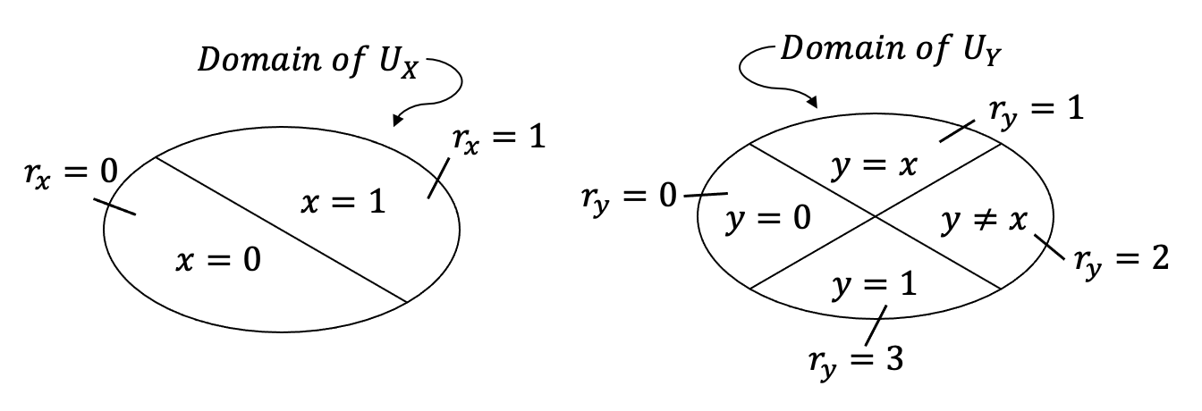
Figure 2: Response function framework for two binary variables $X\rightarrow Y$: only four distinct functions exist from $\mathcal{X}$ to $\mathcal{Y}$, so $\mathcal{U}_{Y}$ can be split accordingly; the discrete response function variable $R_{Y}$ then indicates which of the four regions $U_{Y}$ falls into.

3.1 Response-function reformulation

Since the domains $\mathcal{U}_{i}$ of the exogenous $U_{i}$ are unknown (they could, e.g., be continuous or high-dimensional), we cannot directly parametrise $\mathbb{P}_{\mathbf{U}}$. However, since all $X_{i}$ are assumed discrete, we can reformulate the SCM $\mathcal{M}$ into an equivalent one where the $U_{i}$ are replaced by discrete response function variables $R_{i}$ (Balke and Pearl, 1994). Intuitively, there are only finitely many distinct functions $m_{i}$ that map one discrete domain (that of $\textbf{PA}_{i}$) to another (that of $X_{i}$), and we can think of the $U_{i}$ as (randomly) determining which function is applied. We can therefore partition each $\mathcal{U}_{i}$ into finitely many regions corresponding to these functions, and define a new discrete random variable $R_{i}$ which indicates which region $U_{i}$ falls into (i.e., which response function $m_{i}$ is applied), see Fig. 2 for an illustration.

Formally, we replace the original SCM $\mathcal{M}=(\mathbf{f},\mathbb{P}_{\mathbf{U}})$ from (1) with an equivalent one $\mathcal{M}^{\mathbf{R}}=(\mathbf{m},\mathbb{P}_{\mathbf{R}})$ where the response function variables $\mathbf{R}=(R_{1},...,R_{n})$ with $R_{i}=l_{i}(U_{i})$ index all possible response functions $m_{i}(\cdot,R_{i})$ for each $i$, that is, we rewrite (1) as

$$X_{i}:=f_{i}(\textbf{PA}_{i},U_{i})=f_{i}(\textbf{PA}_{i},l_{i}^{-1}(R_{i}))=f_{i}\circ l_{i}^{-1}(\textbf{PA}_{i},R_{i})=m_{i}(\textbf{PA}_{i},R_{i}),$$ (4)

see Balke and Pearl (1994) for further details. The number of response functions, i.e., the size of the domain $\mathcal{R}_{i}$ for each $R_{i}$ is $|\mathcal{R}_{i}|=K_{i}^{\prod_{X_{j}\in\textbf{PA}_{i}}K_{j}}$ if $\textbf{PA}_{i}$ is not empty, and $|\mathcal{R}_{i}|=K_{i}$ otherwise; we write $\mathcal{R}=\mathcal{R}_{1}\times...\times\mathcal{R}_{n}$.

The advantages of reformulation (4) are twofold: first, unlike for $\mathcal{M}=(\mathbf{f},\mathbb{P}_{\mathbf{U}})$, the structural equations $\mathbf{m}$ of $\mathcal{M}^{\mathbf{R}}$ are known; and second, while unknown, $\mathbb{P}_{\mathbf{R}}$ is a discrete distribution which we can easily parametrise. Any choice of $\mathbb{P}_{\mathbf{R}}$ leads to a fully specified SCM that induces a unique observational distribution and allows for computing counterfactual queries. We can thus minimise (maximise) the counterfactual query (3) over all $\mathbb{P}_{\mathbf{R}}$ which are consistent with the observed $\mathbb{P}_{\mathbf{X}}$ to obtain a lower (upper) bound.

3.2 Bounds for the fully confounded case

First, we consider the fully confounded case (see Fig. 1(c)) following the treatment of Balke and Pearl (1994), adapted to the context of probabilistic causal recourse (2)-(3). Since, in the fully confounded case, $\mathbb{P}_{\mathbf{U}}$ and hence also $\mathbb{P}_{\mathbf{R}}$ do not admit a non-trivial factorisation, we directly parametrise the unknown joint distribution as $q_{\mathbf{r}}=\mathbb{P}_{\mathbf{R}}(\mathbf{R}=\mathbf{r})$. For notational convenience, we also write $p_{\mathbf{x}}=\mathbb{P}_{\mathbf{X}}(\mathbf{X}=\mathbf{x})$, and denote by $\mathbf{p}$ and $\mathbf{q}$ the probability vectors obtained by stacking $p_{\mathbf{x}}$ and $q_{\mathbf{r}}$ for all $\mathbf{r}\in\mathcal{R},\mathbf{x}\in\mathcal{X}$, respectively.

Constraints.

The constraint that $\mathcal{M}^{\mathbf{R}}=(\mathbf{m},\mathbb{P}_{\mathbf{R}})$ needs to be consistent with the observed $\mathbb{P}_{\mathbf{X}}$, i.e., that any $\mathbb{P}_{\mathbf{R}}$ needs to be such that it induces $\mathbb{P}_{\mathbf{X}}$ via $\mathbf{m}$, can be written as

$$\forall\mathbf{x}\in\mathcal{X}:\quad p_{\mathbf{x}}=\sum_{\mathbf{r}\in\mathcal{R}}q_{\mathbf{r}}\prod_{i=1}^{n}\mathbb{I}\{x_{i}=m_{i}(\textbf{pa}_{i},r_{i})\}\,.$$ (5)

Intuitively, the RHS of (5) aggregates the probability of all values $\mathbf{r}$ of $\mathbf{R}$ which give rise to given $\mathbf{x}$; since, generally, $|\mathcal{R}|>|\mathcal{X}|$, there may be multiple such terms. Collecting the products of indicator functions $\mathbb{I}\{\cdot\}$ on the RHS of (5) in a binary $|\mathcal{X}|\times|\mathcal{R}|$ matrix $A$, we obtain $\mathbf{p}=A\mathbf{q}$. Moreover, we have the simplex constraint $\mathbf{q}\in\Delta^{|\mathcal{R}|-1}$.

Objective.

Next, we write the objective to be optimised, i.e., the counterfactual query in (3), for a particular choice of $\mathbb{P}_{\mathbf{R}}$. Note that a counterfactual change to $\mathbf{X}_{\mathcal{I}}$ will not affect the non-descendant variables $\mathbf{X}_{{\text{nd}(\mathcal{I})}}$ which will remain fixed at their factual value $\mathbf{x}^{\texttt{F}}_{\text{nd}(\mathcal{I})}$. For any given $do(\bm{\theta}_{\mathcal{I}})$, we thus only need to reason about changes to the descendant variables $\mathbf{X}_{\text{d}(\mathcal{I})}$. If the set of descendants is empty, we can directly evaluate the classifier and there is no need for bounding. We thus assume that ${\text{d}(\mathcal{I})}$ is not empty. The query (3) can then be written in terms of $\mathbf{q}$ as

$$\mathcal{L}(\mathbf{q};\mathbf{x}^{\texttt{F}},\bm{\theta}_{\mathcal{I}}) =\sum_{\mathbf{x}_{\text{d}(\mathcal{I})}}h\left(\mathbf{x}^{\texttt{F}}_{\text{nd}(\mathcal{I})},\bm{\theta}_{\mathcal{I}},\mathbf{x}_{\text{d}(\mathcal{I})}\right)\mathbb{P}\left(\mathbf{X}_{{\text{d}(\mathcal{I})};do(\bm{\theta}_{\mathcal{I}})}=\mathbf{x}_{\text{d}(\mathcal{I})}|\mathbf{X}=\mathbf{x}^{\texttt{F}}\right)$$ (6)

$$=\frac{1}{p_{\mathbf{x}^{\texttt{F}}}}\sum_{\mathbf{x}_{\text{d}(\mathcal{I})}}h\left(\mathbf{x}^{\texttt{F}}_{\text{nd}(\mathcal{I})},\bm{\theta}_{\mathcal{I}},\mathbf{x}_{\text{d}(\mathcal{I})}\right)\mathbb{P}\left(\mathbf{X}_{{\text{d}(\mathcal{I})};do(\bm{\theta}_{\mathcal{I}})}=\mathbf{x}_{\text{d}(\mathcal{I})},\mathbf{X}=\mathbf{x}^{\texttt{F}}\right)$$

$$=\frac{1}{p_{\mathbf{x}^{\texttt{F}}}}\sum_{\mathbf{x}_{\text{d}(\mathcal{I})}}h\left(\mathbf{x}^{\texttt{F}}_{\text{nd}(\mathcal{I})},\bm{\theta}_{\mathcal{I}},\mathbf{x}_{\text{d}(\mathcal{I})}\right)\sum_{\mathbf{r}\in\mathcal{R}}q_{\mathbf{r}}\left(\prod_{i=1}^{n}\mathbb{I}\left\{x_{i}^{\texttt{F}}=m_{i}\left(\textbf{pa}_{i}^{\texttt{F}},r_{i}\right)\right\}\right)\left(\prod_{i\in{\text{d}(\mathcal{I})}}\mathbb{I}\left\{x_{i}=m_{i}(\textbf{pa}_{i;do(\bm{\theta}_{\mathcal{I}})},r_{i})\right\}\right)$$

where $\textbf{pa}_{i}^{\texttt{F}}$ and $\textbf{pa}_{i;do(\bm{\theta}_{\mathcal{I}})}$ denote the factual and counterfactual (post-intervention) values of $\textbf{PA}_{i}$, respectively.

Optimisation.

To bound the expected outcome (3) of a particular action $do(\bm{\theta}_{\mathcal{I}})$ for a given individual $\mathbf{x}^{\texttt{F}}$, we can then solve the following optimisation problem:

$$\operatorname*{min/max}_{\mathbf{q}\in\Delta^{|\mathcal{R}|-1}}\quad\mathcal{L}(\mathbf{q};\mathbf{x}^{\texttt{F}},\bm{\theta}_{\mathcal{I}})\quad\text{subject to}\quad\mathbf{p}=A\mathbf{q}\,.$$ (7)

Since both objective (6) and constraint (5) are linear in $\mathbf{q}$ and the simplex is convex, (7) is a linear program which can be solved exactly (Schrijver, 1998) and efficiently by linear solvers such as cvxpy (Diamond and Boyd, 2016).

3.3 Bounds for the partially confounded case

In § 3.2, we have directly parametrised the joint distribution $\mathbb{P}_{\mathbf{R}}$, corresponding to the most general case of arbitrary confounding, as shown in Fig. 1(c). However, we may know (e.g., from domain experts) that only a subset of the causal relations are confounded. This case is illustrated in Fig. 1(b) where $X_{1}$ & $X_{2}$ and $X_{2}$ & $X_{3}$ are confounded, but $X_{1}$ & $X_{3}$ are not. Such knowledge can be useful if available as it further constrains the problem and may, in principle, lead to tighter, and thus more informative, bounds. We therefore propose a new formulation for this scenario.

We assume that the partial confounding structure is known. It implies a non-trivial factorisation of $\mathbb{P}_{\mathbf{U}}$, and thus of $\mathbb{P}_{\mathbf{R}}$. For example, Fig. 1(b) implies $\mathbb{P}_{\mathbf{R}}=\mathbb{P}_{R_{1}}\mathbb{P}_{R_{2}|R_{1}}\mathbb{P}_{R_{3}|R_{2}}$. The last term does not depend on $R_{1}$ since $X_{1}$ and $X_{3}$ are unconfounded. This allows to parametrise $\mathbb{P}_{\mathbf{R}}$ with fewer free parameters than in the fully-confounded case from § 3.2. In general, we assume that $\mathbb{P}_{\mathbf{R}}$ factorises as

$$\textstyle\mathbb{P}_{\mathbf{R}}=\prod_{i=1}^{n}\mathbb{P}_{R_{i}|\textbf{PA}(R_{i})}$$ (8)

where $\textbf{PA}(R_{i})\subseteq\mathbf{R}_{1:(i-1)}$ indicates which $X_{1},...,X_{i-1}$ are confounded with $X_{i}$. Instead of the joint distribution, we parametrise each conditional on the RHS of (8) as:

$$\textstyle s_{r_{i},\textbf{pa}(R_{i})}=\mathbb{P}\big{(}R_{i}=r_{i}|\textbf{PA}(R_{i})=\textbf{pa}(R_{i})\big{)}.$$

We then proceed as in the fully confounded case by replacing $q_{\mathbf{r}}$ in the set of constraints (5) and the objective (6) by

$$\textstyle q_{\mathbf{r}}=\mathbb{P}_{\mathbf{R}}(\mathbf{R}=\mathbf{r})=\prod_{i=1}^{n}s_{r_{i},\textbf{pa}(R_{i})}.$$

This leads to a similar optimisation problem to (7), but where we instead optimise over a smaller number of parameters $s_{r_{i},\textbf{pa}(R_{i})}$ specifying valid conditional distributions. However, since the $s_{r_{i},\textbf{pa}(R_{i})}$ appear in the form of products (in both the objective and constraints), the resulting optimisation problem is non-convex and thus more challenging to solve. We discuss possible solutions in § 4.

3.4 Using bounds to inform recourse

For a given $\mathbf{x}^{\texttt{F}}$ and $do(\bm{\theta}_{\mathcal{I}})$, the proposed approaches from § 3.2 and § 3.3 assuming either full (FC) or partial (PC) confounding, respectively, will result in lower (LB) and upper (UB) bounds on (3) that satisfy:

$$\textsc{lb}_{\textsc{fc}}\leq\textsc{lb}_{\textsc{pc}}\leq\mathbb{E}_{\mathbf{U}|\mathbf{x}^{\texttt{F}}}\left[h\left(\mathbf{x}_{do(\bm{\theta}_{\mathcal{I}})}(\mathbf{U})\right)\right]\leq\textsc{ub}_{\textsc{pc}}\leq\textsc{ub}_{\textsc{fc}}$$

where the first and last inequality should generally be strict (i.e., the PC bounds tighter) if knowledge about a non-trivial partial confounding structure is available. Since the aim of recourse is to find actions $do(\bm{\theta}_{\mathcal{I}})$ that would result in a changed prediction ($h>0.5$), we are mainly interested in the lower bounds. In line with (2), we could, for example, choose to recommend the lowest cost action for which the expected outcome is guaranteed to be larger than $0.5$ (or $0.5+\epsilon$ to be more conservative). Alternatively, we could present $\mathbf{x}^{\texttt{F}}$ with the bounds and costs for each action to enable a more informed decision. Finally, we note that here we chose to bound the expected prediction w.r.t. the unknown (and unidentifiable) counterfactual distribution, meaning that recourse is only guaranteed on average if $\text{LB}>0.5$. To be more conservative, we could also bound the worst case outcome by replacing the sum over all possible $\mathbf{x}_{\text{nd}(\mathcal{I})}$ in (6) with a minimum instead

4 Discussion

Discrete variables.

The bounding approach to recourse proposed in the present work requires discrete variables for the response function reformulation and parametrisation of the unobserved distribution. If continuous variables are present, these can either be discretised, or treated separately, either via additional structural assumptions (Karimi et al., 2020b) or by extending recent advances in bounding for continuous outcomes (Kilbertus et al., 2020).

Computational constraints.

The number of response functions grows very quickly for densely connected graphs (i.e., larger $|\textbf{PA}_{i}|$) and with the number of states of the observed variables (i.e., larger $|\mathcal{X}_{i}|$). Moreover, complex confounding structures require more parameters to specify $\mathbb{P}_{\mathbf{R}}$. Computational scalability is a fundamental challenge for computing bounds, which makes this approach currently only feasible for few observed variables with few states.

Optimisation approaches for partial confounding.

A promising approach to solve the non-convex optimisation problem resulting from the partially confounded case (§ 3.3) appears to be a reformulation in which pairs of $s_{r_{i},\textbf{pa}(R_{i})}$ are defined as auxiliary variables, leading to a mixed integer quadratic program which can be solved with bilinear solvers using a branch and bound algorithm as provided, e.g., in gurobi (Gurobi Optimization, 2018). A study of optimality guarantees is relevant for future work.

Preliminary experimental evidence.

Preliminary experimental evidence suggests that the proposed bounding approach can be useful in that—for some combinations of $h$, $\mathbb{P}_{\mathbf{X}}$, and $\mathbf{x}^{\texttt{F}}$, and under unobserved confounding—actions are found for which the lower bound on the expected outcome is larger than 0.5. Moreover, for the partially confounded case, the obtained bounds are typically tighter than those based on assuming full confounding. We leave a more thorough empirical investigation for future work.

5 Conclusion

We proposed the first approach for causal algorithmic recourse in the presence of unobserved confounding. While counterfactuals are unidentifiable in this case, the expected outcome of recourse actions can be bounded subject to constraints from the observational distribution, provided that all observed variables are discrete. In the fully confounded case, this leads to a well known formulation as a linear program which can be solved exactly. When domain knowledge about a partial confounding structure is available, we propose a new formulation that takes this information into account to obtain tighter bounds. Since the resulting optimisation problem is non-convex, it remains an open question how best to tackle it. More efficient algorithmic solutions and potential applications to fairness (Gupta et al., 2019; von Kügelgen et al., 2020) constitute interesting directions for future work.

References

- Balke and Pearl (1994) Alexander Balke and Judea Pearl. Counterfactual probabilities: computational methods, bounds and applications. In Proceedings of the Tenth International Conference on Uncertainty in Artificial Intelligence, pages 46–54, 1994.
- Chouldechova (2017) Alexandra Chouldechova. Fair prediction with disparate impact: A study of bias in recidivism prediction instruments. Big data, 5(2):153–163, 2017.
- Diamond and Boyd (2016) Steven Diamond and Stephen Boyd. Cvxpy: A python-embedded modeling language for convex optimization. The Journal of Machine Learning Research, 17(1):2909–2913, 2016.
- Finkelstein (2020) Noam Finkelstein. Partial identifiability in discrete data with measurement error. arXiv preprint arXiv:2006.06366, 2020.
- Gupta et al. (2019) Vivek Gupta, Pegah Nokhiz, Chitradeep Dutta Roy, and Suresh Venkatasubramanian. Equalizing recourse across groups. arXiv preprint arXiv:1909.03166, 2019.
- Gurobi Optimization (2018) Incorporate Gurobi Optimization. Gurobi optimizer reference manual, 2018.
- Hu et al. (2021) Yaowei Hu, Yongkai Wu, Lu Zhang, and Xintao Wu. A generative adversarial framework for bounding confounded causal effects. 2021.
- Karimi et al. (2020a) Amir-Hossein Karimi, Gilles Barthe, Bernhard Schölkopf, and Isabel Valera. A survey of algorithmic recourse: definitions, formulations, solutions, and prospects. arXiv preprint arXiv:2010.04050, 2020a.
- Karimi et al. (2020b) Amir-Hossein Karimi, Julius von Kügelgen, Bernhard Schölkopf, and Isabel Valera. Algorithmic recourse under imperfect causal knowledge: a probabilistic approach. In Advances in Neural Information Processing Systems, volume 33, pages 265–277, 2020b.
- Karimi et al. (2021) Amir-Hossein Karimi, Bernhard Schölkopf, and Isabel Valera. Algorithmic recourse: from counterfactual explanations to interventions. In Proceedings of the 2021 ACM Conference on Fairness, Accountability, and Transparency, pages 353–362, 2021.
- Kilbertus et al. (2020) Niki Kilbertus, Matt J Kusner, and Ricardo Silva. A class of algorithms for general instrumental variable models. arXiv preprint arXiv:2006.06366, 2020.
- Mahajan et al. (2019) Divyat Mahajan, Chenhao Tan, and Amit Sharma. Preserving causal constraints in counterfactual explanations for machine learning classifiers. arXiv preprint arXiv:1912.03277, 2019.
- Manski (1990) Charles F Manski. Nonparametric bounds on treatment effects. The American Economic Review, 80(2):319–323, 1990.
- Pearl (2009) Judea Pearl. Causality. Cambridge university press, 2009.
- Peters et al. (2017) Jonas Peters, Dominik Janzing, and Bernhard Schölkopf. Elements of causal inference: foundations and learning algorithms. The MIT Press, 2017.
- Richardson et al. (2014) Amy Richardson, Michael G Hudgens, Peter B Gilbert, and Jason P Fine. Nonparametric bounds and sensitivity analysis of treatment effects. Statistical science: a review journal of the Institute of Mathematical Statistics, 29(4):596, 2014.
- Sachs et al. (2020) Michael C Sachs, Erin E Gabriel, and Arvid Sjölander. Symbolic computation of tight causal bounds. arXiv preprint arXiv:2003.10702, 2020.
- Schrijver (1998) Alexander Schrijver. Theory of linear and integer programming. John Wiley & Sons, 1998.
- Ustun et al. (2019) Berk Ustun, Alexander Spangher, and Yang Liu. Actionable recourse in linear classification. In Proceedings of the Conference on Fairness, Accountability, and Transparency, pages 10–19, 2019.
- Venkatasubramanian and Alfano (2020) Suresh Venkatasubramanian and Mark Alfano. The philosophical basis of algorithmic recourse. In Proceedings of the 2020 Conference on Fairness, Accountability, and Transparency, pages 284–293, 2020.
- von Kügelgen et al. (2020) Julius von Kügelgen, Amir-Hossein Karimi, Umang Bhatt, Isabel Valera, Adrian Weller, and Bernhard Schölkopf. On the fairness of causal algorithmic recourse. arXiv preprint arXiv:2010.06529, 2020.
- Wachter et al. (2017) Sandra Wachter, Brent Mittelstadt, and Chris Russell. Counterfactual explanations without opening the black box: Automated decisions and the gdpr. Harv. JL & Tech., 31:841, 2017.
- Wu et al. (2019) Yongkai Wu, Lu Zhang, Xintao Wu, and Hanghang Tong. Pc-fairness: A unified framework for measuring causality-based fairness. In Advances in Neural Information Processing Systems, pages 3404–3414, 2019.
- Zhang and Bareinboim (2021a) Junzhe Zhang and Elias Bareinboim. Non-parametric methods for partial identification of causal effects. https://causalai.net/r72.pdf, 2021a.
- Zhang and Bareinboim (2021b) Junzhe Zhang and Elias Bareinboim. Bounding causal effects on continuous outcome. In Proceedings of the 35nd AAAI Conference on Artificial Intelligence, 2021b.