Distribution of the order parameter in strongly disordered superconductors: analytic theory

Abstract

We developed an analytic theory of inhomogeneous superconducting pairing in strongly disordered materials, which are moderately close to superconducting-insulator transition. Single-electron eigenstates are assumed to be Anderson-localized, with a large localization volume. Superconductivity develops due to coherent delocalization of originally localized preformed Cooper pairs. The key assumption of the theory is that each such pair is coupled to a large number $Z\gg 1$ of similar neighboring pairs. We derived integral equations for the probability distribution $P\left(\Delta\right)$ of local superconducting order parameter $\Delta\left(\boldsymbol{r}\right)$ and analyzed their solutions in the limit of small dimensionless Cooper coupling constant $\lambda\ll 1$. The shape of the order-parameter distribution is found to depend crucially upon the effective number of "nearest neighbors" $Z_{\text{eff}}=2\nu_{0}\Delta_{0}Z$, with $\nu_{0}$ being the single-particle density of states at the Fermi level. The solution we provide is valid both at large and small $Z_{\text{eff}}$; the latter case is nontrivial as the function $P\left(\Delta\right)$ is heavily non-Gaussian. One of our key findings is the discovery of a broad range of parameters where the distribution function $P\left(\Delta\right)$ is non-Gaussian but also non-critical (in the sense of SIT criticality). The analytic results are supplemented by numerical data, and good agreement between them is observed.

I Introduction

Strongly disordered superconductors are interesting both from fundamental and practical perspectives. The fundamental problem of a quantum (zero-temperature) phase transition between superconducting and insulating ground states (Superconductor-Insulator transition, or SIT) attracted considerable attention since mid-80’s (Goldman89, ; Fisher90, ; Shahar97, ; Fazio2001, ; Gantmakher2010, ) and got an additional burst of research during the last decade. Prominent examples include various structurally different realizations of the SIT, such as granular arrays of Josephson Junctions or thick homogeneous films of amorphous Indium Oxide. The whole variety of phenomena collectively labeled as SIT demonstrate a great deal of diversity in the underlying physics and thus cannot be possibly explained by a single mechanism (see the recent review (SFK-review-2020, ) for further details). In this paper, we theoretically demonstrate several rather persistent properties of 3D materials with homogeneous structure and strong microscopic disorder.

The practical side of interest to strongly disordered superconductors stems from potential applications in quantum computing technologies in the form of so called “superinductors” (Doucot12, ; Kitaev13, ; Groszowski18, ; Mooij05, ; Mooij06, ). These are much wanted yet so far mostly hypothetical inductive devices that combine nearly absent dissipation at low energies (in GHz range) with high inductance and small spatial size such that kinetic inductance per square $L_{\square}$ exceeds $10\text{ nH}$. The principal opportunity to fabricate such a device is provided by the platform of thick films of strongly disordered superconductors. Indeed, the latter feature low superfluid density $\rho_{s}$ and the associated high kinetic inductance per square $L_{\square}\sim 1/\rho_{s}$, enabling one to implement an superinductor within a compact geometry. Such extreme values for these materials are a consequence of high normal state resistance induced by disorder (Tinkham_supercond-textbook, , sec. 3.10)(Sacepe_subgap-excitations_APS-Meeting-March-2021, )(sherman2015higgs_for-disorder-driven-suppresion-of-rho-s, , Fig. 3b, 3c in particular). On the other hand, the necessity for the absence of low-energy dissipation requires one to use materials with a well resolved gap in the optical excitation spectrum — a feature so natural for superconducting materials.

However, it occurs that the two conditions mentioned above (low $\rho_{s}$ and absence of any low-energy excitations) come into conflict. Superconductors which are too close to SIT unavoidably contain some non-zero density of low-lying collective modes even when single-electron density of states (1-DoS) is fully gapped, as it is demonstrated by theoretical analysis (Feigelman_Microwave_2018, ) and experimental observations (Sacepe_subgap-excitations_APS-Meeting-March-2021, ). Yet, the question of low-energy modes in strongly disordered superconductors is by no means resolved qualitatively. The preliminary analysis performed in paper (Feigelman_Microwave_2018, ) was based upon the approximation of constant superconducting order parameter $\Delta(\mathbf{r})=\Delta$, which is far from being obviously correct. Instead, a self-consistent theory of the system’s collective modes without the use of such a drastic approximation is needed. Moreover, the spatial distribution of superconducting order parameter can now be probed by means of modern low-temperature Scanning Tunneling Microscopy methods (Sacepe10, ; Sacepe_2011_for-pair-preformation, ; Kamlapure12, ; Ganguly17, ; Tamir_private, ). It is thus of both fundamental and practical interest to develop a theory that would be able to: 1) describe realistic spatial distributions of the order parameter, and 2) describe the behavior of collective modes on top of the spatially inhomogeneous superconducting state. In the present paper we deal with the first of these problems only, leaving the second one for the near future.

The local probability distribution function $P(\Delta)$ of superconducting order parameter has already been addressed in several important limiting cases of disorder strength. The limit of small disorder corresponds to usual dirty superconductors with diffusive transport in normal state. For this regime, the structure of statistical fluctuations of the order parameter was analyzed in the seminal paper (L0_1972, , see Sec. 3 in particular) by means of semiclassical theory of superconductivity, demonstrating a narrow purely Gaussian $P\left(\Delta\right)$. In the opposite limit of small disorder, the single-electron wave functions suffer Anderson localization transition, rendering the conventional semiclassical approach inapplicable. To describe this regime, the work (Ioffe_2010_ref-about-Onsager, ) substantiated the model on the Bethe lattice, while the subsequent paper (Feigelman_SIT_2010, ) showed that the resulting $P\left(\Delta\right)$ exhibits critical features, such as “fat tails” extended to the region of large $\Delta$, much larger than the typical value $\Delta_{\text{typ}}$. However, realistic experiments usually deal with superconducting samples which fall within neither of the two limiting cases described above; it is especially so for superconductors which may serve as candidates for construction of superinductors. On the one hand, superconducting materials discussed in the work are much more disordered than usual dirty superconductors, to the extent where neither the standard semiclassical theory of Ref. (L0_1972, ) nor even the mere Gaussian approximation for $P\left(\Delta\right)$ are applicable. As suggested by numerical data (Randeria01, ; Bouadim11, ) and experimental observations (Sacepe_2011_for-pair-preformation, ; Lemarie2013, ; Tamir_private, ), this type of materials features heavily non-Gaussian profiles of the order parameter distribution. On the other hand, the level of disorder, the resulting non-critical distribution $P\left(\Delta\right)$ and the requirement for the absence of low-energy excitations are all suggesting that the samples of interest are somewhat away from the SIT, so that the the critical theory of Ref. (Feigelman_SIT_2010, ) is also inapplicable. The present paper is devoted to the development of analytical methods able to study the order parameter distribution in the materials that belong to the region in between the two limiting cases. The latter turns out to be parametrically broad, as we also show below. While our approach is general and valid in principle at all temperatures, in this paper we consider $T=0$ limit only.

This paper is organized as follows. We formulate our theoretical model in II. Within it, we review the relevant phenomenology of disordered superconductors and formulate the Hamiltonian of the system. The corresponding static self-consistency equations for the order parameter are then introduced along with a brief discussion of applicability and several known limits. The section is closed by a brief discussion of the methods used in previous works to analyze problems similar to the one stated in the present work. III then presents the body of our theoretical approach. In III.1, we start by deriving a general set of equations to describe the statistics of solution to systems of local nonlinear equations with disorder, such as the self-consistency equations for the order parameter. Within the following III.2, those equations are substantially simplified in the physically relevant limit of small order parameter $\nu_{0}\Delta_{0}\ll 1$ and large number of neighbors $Z\gg 1$ within the localization volume of a given single-particle state. Such simplifications render the presented equations amenable for both numerical and analytical analysis. In III.3, the reader can find an explicit analytical solution to the the proposed equations on the distribution function of the order parameter and related quantities in terms of certain special functions. The following III.5 then briefly describes the numerical routines used to analyze both the original self-consistency equations in a particular realization of disorder in the system and the derived equations on the distributions of various physical quantities across different disorder realizations. In III.6 we demonstrate the key outcomes of our theoretical analysis: the profile of the distribution function as a function of the parameters of the model and the asymptotic behavior of the distribution. The subsection also contains some results for the distribution of other local physical quantities. III.7 then introduces and analyzes several important extensions of our model that allow us to draw conclusions about the robustness of our findings. Finally, IV summarizes the key theoretical achievements and outlines several immediate developments. This paper is accompanied by the Supplementary Materials (SM) (SM, ) that contain additional technical information on various steps of theoretical and numerical analysis employed in this work.

II The model

II.1 Phenomenology of strongly disordered superconductors

The physics of superconductor-insulator transition (SIT) owes its rich phenomenology to the underlying complexity of the Anderson Localization transition in the single-particle spectrum of the system. The paper (Feigelman_Fractal-SC_2010, ) conducts an extensive research of the topic, building upon the seminal paper (Ma_Lee_1985_Ref-to-pseudospins, ) and early numerical studies (Randeria01, ); here we employ a simplified description proposed and substantiated in Ref.-s (Ioffe_2010_ref-about-Onsager, ; Feigelman_SIT_2010, )

The single-particle electron states are described by spatially localized wave-functions $\psi_{i}\left(r\right)$ with large localization volume $V_{\text{loc}}$ and complex spatial structure (Feigelman_Fractal-SC_2010, , Sec. 2). The single-particle eigenenergies $\xi_{i}$ of these states can be approximated as randomly distributed independent variables, with the typical width of the distribution $\nu\left(\xi\right)$ being of order of the Fermi energy $E_{F}$. We assume that this distribution arranges a finite density of states per spin projection $\nu_{0}=\nu\left(\xi=0\right)\sim 1/E_{F}$ at the Fermi level.

Even prior to the emergence of the global superconducting coherence, the systems in question are known to favor the formation of localized Cooper pairs (Feigelman_Fractal-SC_2010, , Sec. 3 and ref. therein). This phenomenon can be delineated by an additional energy $E_{\text{PG}}$ per each unpaired electron in the system. For the systems of interest, the typical scale of $E_{\text{PG}}$ is significantly larger than all superconducting energy scales (Feigelman_Fractal-SC_2010, , Sec. 4.3). Consequently, single-particle excitations barely contribute to low-energy physics. One is thus able to describe the relevant physics by considering only the states corresponding to presence or absence of a local Cooper pair on a given single-particle state $i$, effectively halving the Hilbert space, as described in (Feigelman_Fractal-SC_2010, , Sec. 6).

The superconducting order in the system then corresponds to coherent delocalization of preformed Cooper pairs, as demonstrated experimentally in Ref. (Sacepe_2011_for-pair-preformation, ) and supported by numerical data (Bouadim11, ). Such behavior results from attractive Cooper-like pairwise interaction between the Cooper pairs. This interaction is assumed to be local, so that it only connects single-particle states with a finite spatial overlap. As a result, each single-particle state $i$ is effectively interacting with other states located within the localization volume of $i$. However, the particular subset of those states is rather nontrivial due to both the complex structure of the single-particle wave-functions $\psi_{i}\left(r\right)$ and explicit dependence of the matrix element of the interaction on energy difference $\xi_{i}-\xi_{j}$ between the interacting states. To describe the emerging phenomenology, we employ a simplistic model of the spatial structure of matrix elements that assumes each single-particle state $i$ to be effectively connected to a constant number $Z$ of states chosen at random from within the localization volume of $i$. The value of $Z$ can be estimated as a small fraction of the total number of states within the localization volume that has significant spatial overlap with a given state $i$, so that $Z\sim nV_{\text{loc}}\cdot\eta$, where $n$ is the electron concentration and $\eta$ is a small numerical factor. Due to the proximity to the Anderson transition, the localization volume $V_{\text{loc}}$ is large (Feigelman_Fractal-SC_2010, , Sec. 2), thus also rendering $Z\gg 1$, even despite the smallness provided by $\eta$. We note, however, that for the analysis presented below it is only important that $Z$ itself is a large quantity. In particular, the analysis of a model where each site has the value of $Z$ distributed according to Poisson distribution suggest that the fluctuations of $Z$ do not play a significant role in the observed behavior.

In what follows, we will also retain the information about the energy dependence $D\left(\xi_{i}-\xi_{j}\right)$ of the matrix elements of the interaction. This energy dependence is primarily characterized by the large energy cutoff $\varepsilon_{D}$ that is typically of the order of the Debye energy of phonons. Due to this energy scale, the interaction between the states with energy difference $\left|\xi_{i}-\xi_{j}\right|$ larger than $\varepsilon_{D}$ is essentially absent. On the other hand, we assume that the localization volume of single-particle electron states is large enough to secure the continuity of phonon spectrum, i.e. $\delta_{\text{loc}}\ll\varepsilon_{D}$, with $\delta_{\text{loc}}$ being the characteristic phonon level spacing in the localization volume. It is worth mentioning that the actual profile of $D$ for dirty superconductors with pseudogap is known to exhibit substantial dependence at small energies due to the underlying phenomenology of Anderson insulator (Feigelman_Fractal-SC_2010, , Sec. 4). This feature presents an additional complication which does not seem to be universally relevant. We will thus simplify the model below by assuming that $D$ is smooth in the vicinity of the zero energy difference and arranges a small static coupling constant $D\left(0\right)$. The latter is then conventionally parametrized by small dimensionless Cooper constant $\lambda\ll 1$ as $D\left(0\right)=\lambda/\left(2\nu_{0}Z\right)$, where the multiplier $Z$ in the denominator ensures proper normalization of the matrix element.

An important issue is related to the spatial geometry of the manifold spanned by the indices of eigenstates $i,j,...$, etc. On the one hand, the eigenstates $\psi_{i}\left(\boldsymbol{r}\right)$ are supposed to be localized in the physical 3D space (or in the effectively 2D space in case of very thin films), and the locations $R_{i}$ of the maxima in the absolute values $\left|\psi_{i}\left(\boldsymbol{r}\right)\right|$ constitute a set of points in real 3D (or 2D) space. On the other hand, the major role in the formation of the superconducting state is played specifically by the eigenstates close to the Fermi-level and in addition also sufficiently strongly coupled to each other. Since coupling amplitudes between eigenstates near the mobility edge strongly vary in magnitude, only small fraction of all eigenstates $\psi_{j}\left(\boldsymbol{r}\right)$ that can be found around the selected one — $\psi_{i}\left(\boldsymbol{r}\right)$ — is coupled to $\psi_{i}\left(\boldsymbol{r}\right)$ considerably. The resulting spatial structure of interacting eigenstates can be considered, in some approximation, as a strongly diluted random graph with some large but finite number of neighbors $Z$ per each participating “site”. The crucial feature of this graph — as opposed to the usual Euclidean lattice — is its loopless structure. More exactly, a random graph with coordination number $Z$ that is much smaller than the total number of sites $N$, does contain loops, but their typical size grows with system size as $\sim\ln N/\ln\left(Z-1\right)$, while small loops are nearly absent (bollobas2001random, ). This, in turn, suppresses infra-red fluctuations of the order parameter, which are known to be crucial for the adequate description of thermal phase transitions in low-dimensional systems. On the other hand, in the present problem we are interested in statistical properties of the order parameter at lowest temperatures, where thermal fluctuations are absent anyway. The most important effects to be studied here are due to strong statistical fluctuations (of quenched disorder), which can be considered within the loop-less approximation.

II.2 The model Hamiltonian

The presented phenomenological picture allows us to adopt the following model Hamiltonian of a strongly disordered superconductor on the verge of localization transition and with a well developed pseudogap:

$$H =\sum_{i}\xi_{i}\left(a_{i\downarrow}^{\dagger}a_{i\downarrow}+a_{i\uparrow}^{\dagger}a_{i\uparrow}\right)$$

$$-\sum_{\left\langle ij\right\rangle}D_{ij}\left(a_{i\downarrow}^{\dagger}a_{i\uparrow}^{\dagger}a_{j\uparrow}a_{j\downarrow}+\text{Herm. conj.}\right).$$ (1)

Here, $a_{i\sigma}^{\dagger},a_{i\sigma}$ are fermionic creation and annihilation operators of single-particles states $\psi_{i\sigma}$ obeying standard commutation relations, with $\sigma\in\left\{\uparrow,\downarrow\right\}$ denoting the spin of the electron. The discussed preformation of Cooper pairs reduces the Hilbert space to eigenstates of Cooper pair occupation number

$$n_{i}=\frac{1}{2}\left(a_{i\downarrow}^{\dagger}a_{i\downarrow}+a_{i\uparrow}^{\dagger}a_{i\uparrow}\right)=\left\{0,1\right\},$$ (2)

which is obviously conserved by the Hamiltonian. The first term in Eq. (LABEL:Model-Hamiltonian) then reproduces the randomly distributed independent single-particle energies $\xi_{i}$. The corresponding distribution $\nu\left(\xi\right)$ has a typical width of order of the Fermi energy $E_{F}$. The particular profile of $\nu\left(\xi\right)$ is of little importance for the low-energy physics as long as the single-particle density of states $\nu_{0}=\nu\left(\xi=0\right)$ is finite, i. e. $\nu_{0}\sim 1/E_{F}$. The second term in Eq. (LABEL:Model-Hamiltonian) represents local Cooper-like interaction, with the summation going over all pairs $\left\langle ij\right\rangle$ of effectively interacting single-particle states. We assume that each state $i$ is effectively coupled to a large number $Z\gg 1$ of other localized states. Importantly, the pairs of coupled states are chosen completely at random, so that the resulting structure bears no information about the original 3D nature of the system (as opposed to similar models that are formulated on a lattice, see e.g. the 2D-CMF model of Ref. (Lemarie2013, )), while also preserving some notion of the translation symmetry (in contrast to the models on a portion of the Bethe lattice, as e.g. the one of Ref (Feigelman_SIT_2010, )). The matrix element $D_{ij}$ of the interaction is determined by the energy dependence of the interaction and is modeled by a smooth function with the following asymptotic properties

$$D_{ij}=D\left(\xi_{i}-\xi_{j}\right)\approx\begin{cases}\frac{\lambda}{2\nu_{0}Z},&\left|\xi_{i}-\xi_{j}\right|\apprle\varepsilon_{D},\\ 0,&\left|\xi_{i}-\xi_{j}\right|\apprge\varepsilon_{D},\end{cases}$$ (3)

where $\lambda\ll 1$ is the dimensionless Cooper constant and $\varepsilon_{D}\ll W$ is the characteristic scale of energy dependence of the Cooper interaction.

II.3 The self-consistency equation

The superconducting transition for the Hamiltonian (LABEL:Model-Hamiltonian) is captured by the saddle-point (Bogolyubov) approach. According to it, one approximates the Cooper interaction with coupling to the field of the complex order parameter $\Delta$. The latter is then found as a minimum of the self-consistent free energy. In the absence of time reversal symmetry breaking factors, such as magnetic field or external current, the field of the order parameter $\Delta_{i}$ can be chosen to be real and positive. One then determines the zero temperature configuration of the order parameter as a positive solution to the following self-consistency equation (Feigelman_Fractal-SC_2010, , Sec. 4.3 and Sec. 6.1):

$$\Delta_{i}=\sum_{j\in\partial i}D\left(\xi_{i}-\xi_{j}\right)\frac{\Delta_{j}}{\sqrt{\Delta_{j}^{2}+\xi_{j}^{2}}},$$ (4)

where the summation in the right hand side goes over $Z$ states labeled with index $j$ that interact with a given state $i$. The reader can find the derivation of this equation for the original Hamiltonian (LABEL:Model-Hamiltonian) in A. One then has to solve the equation (LABEL:saddle-point_order-parameter) for a given realization of random energies $\xi_{i}$ and subsequently analyze the statistical properties of the resulting ensemble of $\Delta_{i}$, such as the local probability distribution and the structure of spatial correlations.

However, the conventional self-consistent approach fails to describe the Superconductor Insulator Transition (SIT) itself. Namely, Eq. (LABEL:saddle-point_order-parameter) posses nontrivial solutions for arbitrary weak Cooper coupling strength, while in reality one observes destruction of the global superconducting order at a certain value of the coupling constant (Feigelman_SIT_2010, ). The correct description of the SIT requires careful treatment of the self-action of the order parameter in a form of so-called Onsager reaction term. The papers (Ioffe_2010_ref-about-Onsager, ; Feigelman_SIT_2010, ) provide a consistent account for this effect by means of the cavity method (MezardParisi_cavity0, ; MezardParisi_cavity1, ) and demonstrate the emergence of broad probability distributions of the order parameter with slow power-law decay at large values, thus revealing the defining role of extreme values in the corresponding quantum phase transition. However, the paper (Feigelman_SIT_2010, ) also demonstrates that the effects of self-action are only relevant for $Z\apprle Z_{1}$, where

$$Z_{1}=\lambda\exp\left\{\frac{1}{2\lambda}\right\},$$ (5)

with $\lambda\ll 1$ being the dimensionless Cooper coupling constant. Away from this region the reaction term constitutes only a small correction, rendering the self-consistency equation (LABEL:saddle-point_order-parameter) applicable. We will thus limit our analysis to the case $Z\apprge Z_{1}$, although our technique could be extended to include the Onsager reaction term. Despite the introduced limitation, we report a broad region of $Z$ values for which the distribution of the order parameter still assumes substantially non-Gaussian profile indicative of the competition between strong fluctuations and global superconducting order.

II.4 Mean-field solution

The typical scale of the order parameter in Eq. (LABEL:saddle-point_order-parameter) can be established by a simple mean-field approach. Namely, one seeks a spatially uniform solution $\Delta_{i}=\Delta_{0}=\text{const}$, approximating the right-hand side of the self-consistency equation (LABEL:saddle-point_order-parameter) by its statistical average. This substitution is justified a priori for sufficiently large values of $Z$ by virtue of the central limit theorem. As suggested by the seminal paper (Ma_Lee_1985_Ref-to-pseudospins, ), a physical estimate for the relevant range of $Z$ could be obtained by demanding that each single-particle state has at least one other resonant state within the energy interval of size $\Delta_{0}$. This results on the following criteria:

$$Z\apprge Z_{2}=\frac{1}{2\nu_{0}\Delta_{0}}\sim 2\nu_{0}\varepsilon_{D}\cdot e^{1/\lambda}.$$ (6)

In this case, one can neglect the fluctuations of the right hand side of Eq. (LABEL:saddle-point_order-parameter) around its mean value and obtain:

$$\Delta_{0}\left(\xi_{0}\right)=Z\left\langle\frac{\Delta_{0}\left(\xi\right)}{\sqrt{\Delta_{0}^{2}\left(\xi\right)+\xi^{2}}}\cdot D\left(\xi-\xi_{0}\right)\right\rangle_{\xi},$$ (7)

where $\left\langle\bullet\right\rangle_{\xi}$ denotes the statistical distribution w.r.t the distribution of $\xi$. The equation still contains the value $\xi_{0}$ of the disorder field at a given site, reflecting the fact that the order parameter is itself a function of onsite energy $\xi_{0}$.

The value of $\Delta_{0}$ is found self-consistently by solving the resulting integral equation. The smallness of the coupling $D\left(\xi\right)\sim\lambda/\left(2\nu_{0}Z\right)$ at small energies $\left|\xi\right|\ll\varepsilon_{D}$ enables one to provide an analytical solution for the order parameter close to the Fermi surface in a form of the celebrated BCS expression:

$$\Delta_{0}\left(\xi_{0}=0\right)=2E_{0}\cdot\exp\left\{-\frac{1}{\lambda}\right\},$$ (8)

where the value of $E_{0}\sim\varepsilon_{D}$ is expressed via the single-particle density of states $\nu\left(\xi\right)$ and the exact profile of the $D$ function. The explicit form for $E_{0}$ is presented in A.

As this point, it is worth introducing one more microscopic parameter that turn out to play the defining role for the distribution of the order parameter:

$$\kappa=\frac{\lambda}{Z/Z_{2}}\equiv\frac{D\left(0\right)}{\Delta_{0}}$$ (9)

Qualitatively, this parameter combines the information about the criteria (LABEL:Z2) and the strength of the attractive interaction in the form of the dimensionless coupling constant $\lambda$. Otherwise, the value of $\kappa$ bears the meaning of properly rescaled matrix element of bare attractive interaction. A particularly important aspect of this parameter is that it quantifies the competition between the superconducting pairing and the disorder. The former enters the expression via the value of the bare matrix element of the attraction, and the latter is represented by the mean field of the order parameter which is defined by the distribution of the onsite disorder according to Eq. (LABEL:mean-field_order-parameter_eq).

While our analysis shows that the mean-field result (LABEL:mean-field-delta_zero-temp) is only justified for $Z\apprge Z_{2}$, the exponential smallness of the actual order parameter rests solely on the smallness of the coupling constant $\lambda$. This makes $\Delta_{0}$ a valid scale to describe the typical magnitude of the true solution to the self-consistency equation (LABEL:saddle-point_order-parameter) in the whole range $Z\apprge Z_{1}$ we are interested in. Below we find distribution function $P\left(\Delta\right)$ and show that it can be strongly non-Gaussian in general, while narrow Gaussian shape is realized if the inequality (LABEL:Z2) is satisfied.

II.5 Relation to previous studies

Our analytical approach presented below in III borrows certain features from the methods that are widely used to analyze statistical physics of disordered systems on the Bethe lattice. The latter is defined as an infinite tree with all but one vertices having $Z-1$ descendants and one ancestor, while the root site has $Z$ descendants and no ancestor, so that each vertex has exactly $Z$ neighbors in total. One of the key properties of the Bethe lattice is the absence of loops which enables one to derive recursive relations for both a given local quantity itself and distribution function of this quantity across various disorder realizations. Qualitatively, such possibility can be perceived as a consequence of the fact that in a system with no loops any two non-overlapping subsystems are connected by a single chain of sites that arranges the exchange of statistical information and thus induces statistical correlations. This allows one to analyze the statistical properties of the system by considering the state of just a single site. A prominent exploitation of this feature was provided by M. Mezard and G. Parisi within their analysis of spin glass problems on the Bethe lattice (MezardParisi_cavity0, ; MezardParisi_cavity1, ) by means of the “cavity method”. A similar approach was used in Ref. (Feigelman_SIT_2010, ) for a model of strongly disordered superconductor that is structurally similar to the one used in the present work.

However, one should be careful when using a finite portion of the Bethe lattice as a model for any physical system. The issue is that truncating the Bethe lattice explicitly breaks the equivalence between different vertices in the system and thus induces a certain preferred direction in the system. Precisely for this reason we use the ensemble of Random Regular Graphs (RRGs) and its generalizations as a finite size approximation to the Bethe lattice. The important difference between the two structures is that a typical RRG inevitably contains large loops with lengths of the order of the graph’s diameter $D\sim\ln N/\ln\left(Z-1\right)$ that serve to restore the translation symmetry in the system (bollobas2001random, ). Remarkably, our theoretical and numerical analysis shows that as long as the number of neighbors $Z$ of each site is large enough and the disorder is not critically strong (in the sense of the vicinity of the SIT), neither the presence of even short loops nor even the irregularity of the base graph (in the sense that each site might have different number of neighbors) have any noticeable influence on the distribution of the order parameter.

It is worth discussing two more subtle differences between our present approach and the one used previously in Ref. (Feigelman_SIT_2010, ). The cavity method (MezardParisi_cavity0, ; MezardParisi_cavity1, ) was developed originally for Ising-type problems. Relying on the exact recursive relation for the conditional partition function, it derives its power from the possibility to parametrize the latter in terms a “local field” $h_{i}$ defined for each site of the problem. This is possible for the classical Ising problem where only two classical states per site are present. Upon taking into account the normalization condition we are left with only one real number $h_{i}$ that parametrizes the conditional partition function. Our superconducting problem is different in two aspects. One of them is due to the quantum nature of local degrees of freedom, as it was already discussed in (Feigelman_SIT_2010, ). Namely, the Hamiltonian (LABEL:Model-Hamiltonian) can be exactly mapped on the spin $1/2$ $XY$ model in transverse field, with the corresponding spin degrees of freedom termed pseudospins (Ma_Lee_1985_Ref-to-pseudospins, ). Ref. (Feigelman_SIT_2010, ) then uses the “static approximation” that neglects dynamic correlations between pseudospins. The second feature (left unnoticed in Ref. (Feigelman_SIT_2010, )) is that, even with quantum effects neglected, the conditional partition function for a spin $1/2$ degree of freedom with $XY$ symmetry cannot be parametrized, in general, by a single complex field $\Delta_{i}$.

A generalization of the cavity method is certainly possible for this type of order parameter as well, but it is more involved. The difference between the cavity mapping used in Ref. (Feigelman_SIT_2010, ) and the exact one becomes important once the terms nonlinear in the magnitude of the order parameter become essential for physics. We expect that the recursive equations derived and analyzed in Ref. (Feigelman_SIT_2010, ) are exact (leaving aside the additional problem with the accuracy of “the static approximation”) as long as the amplitude of the order parameter is small in some appropriate sense. For example, the linearized form of these equations is perfectly suitable, e. g., for the analysis of the temperature-driven transition. It is also correct to use the recursive equations of Ref. (Feigelman_SIT_2010, ) for the analysis of the long tail of the order parameter distribution, as the effects of nonlinearity are also weak in this case. In the present paper we are interested in the shape of the complete distribution function $P\left(\Delta\right)$ at $T=0$, where the effects of nonlinearity are strong. Thus here we prefer to employ classical form of the self-consistency equations (LABEL:saddle-point_order-parameter); as explained in the previous Subsection, the related inaccuracy (as long as we do not include Onsager reaction term) is small as the ratio $Z_{1}/Z\ll 1$.

III Distribution of the order parameter

In this section, we present both analytical and numerical results for the onsite joint probability distribution of fields $\xi$ and $\Delta$ on a given site. The latter is defined as

$$P_{i}\left(\xi,\Delta\right)=\left\langle\delta\left(\xi-\xi_{i}\right)\delta\left(\Delta-\Delta_{i}\left(\left\{\xi\right\}\right)\right)\right\rangle,$$ (10)

where $\delta\left(x\right)$ is the Dirac $\delta$-function, $\Delta_{i}\left(\left\{\xi\right\}\right)$ is the exact solution of the self-consistency equation (LABEL:saddle-point_order-parameter) for a given realization of the disorder field $\xi$, and the average $\left\langle\bullet\right\rangle$ is performed over all configurations of the $\xi$ field. The distribution is normalized by definition:

$$\intop_{0}^{\infty}d\Delta^{\prime}\,P\left(\xi,\Delta^{\prime}\right)=\nu\left(\xi\right),$$ (11)

where $\nu\left(\xi\right)$ is the distribution of the original onsite disorder field $\xi$.

III.1 Equation on the distribution in a locally tree-like system

Within our model, each single-particle state $i$ is effectively interacting with $Z$ other single-particle states selected at random. The corresponding structure of the matrix elements can be represented by an instance of so called Random Regular Graphs. The latter are known to exhibit vanishing concentration of finite loops in the thermodynamical limit (McKay_1981, ). In other words, the sites at distances up to some large distance $d$ from any chosen site $i$ form a regular loop-free structure rooted at $i$ with probability approaching unity as the total number of sites $N$ tends to infinity. A fragment of the corresponding structure termed locally tree-like is illustrated on 1.

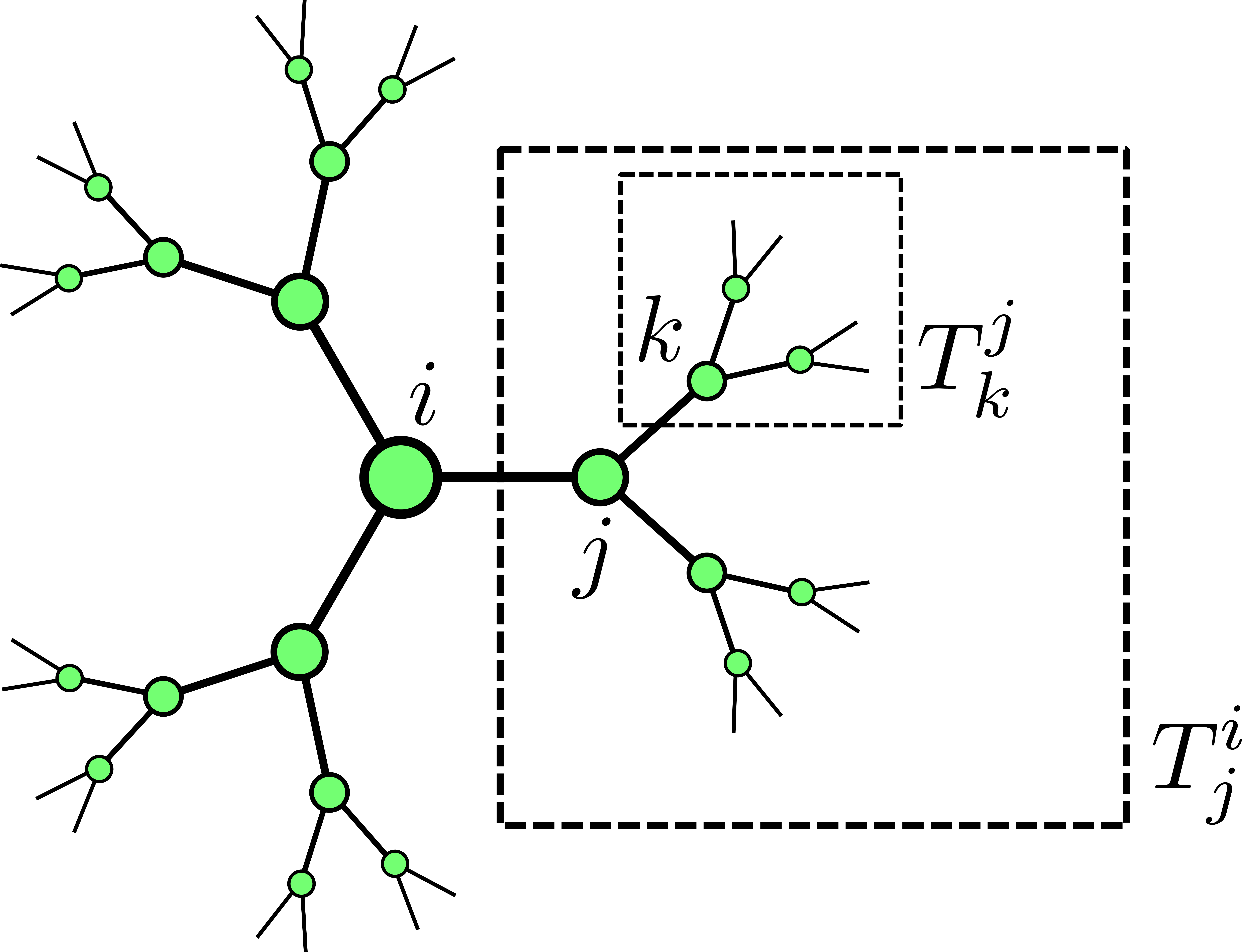
Figure 1: A schematic illustration of the neighborhood of radius $d=3$ of a particular vertex $i$ of a Random Regular Graph (RRG) of degree $Z=3$, i. e with each vertex having exactly three neighbors. Large RRGs are known to exhibit vanishing concentration of short loops (McKay_1981, ), so that up to some large distance $d$ the neighborhood of $i$ represents a loop-free structure, i. e. a tree. In particular, each neighboring vertex $j$ is a root of the corresponding branch $T_{j}^{i}$ consisting of all vertices that can be reached from $i$ by a path containing at most $d$ edges. Because the whole neighborhood is a tree, such path is unique. Similarly, each nearest neighbor of $j$ except $i$ itself is also a root of a tree $T_{k}^{j}$ nested in $T_{j}^{i}$. Such a nested structure is convenient for various recursive considerations.

For the physical system in question, one expects that the spatial distribution of the order parameter exhibits a finite correlation radius, at least away from the SIT. This implies that the value of the order parameter at a given site is only sensitive to the characteristics of neighboring sites up to some finite correlation distance $d_{0}$ away from the chosen site. In conjunction with the locally tree-like structure, this property suggests that for each site $i$ the neighboring sites $j\in\partial i$ are only correlated via the site $i$ itself. Indeed, the underlying graph only contains large loops that are much longer than the correlation length $d_{0}$, and thus cannot influence distributions of any local quantities.

To make use of the described properties, we consider the system where the values of both $\xi$ and $\Delta$ at a given site $i$ are fixed externally, i. e. $\Delta_{i_{0}}=\Delta_{0}$ and $\xi_{i_{0}}=\xi_{0}$, as opposed to finding $\Delta_{i}$ from the self-consistency equations (LABEL:saddle-point_order-parameter) for site $i$. Now, consider a nearest neighbor $j\in\partial i$ of the “quenched” site $i$. Due to the aforementioned structure of spatial correlations, the exact solution $\Delta_{j}^{i}\left(\left\{\xi\right\}|\xi_{0},\Delta_{0}\right)$ to the modified version of the self-consistency equations (LABEL:saddle-point_order-parameter) depends considerably only on the values of the disorder field $\xi$ within some finite region $T_{j}^{i}$ rooted at $j$, see 1. Crucially, the described locally tree-like structure implies that for different $j$ the corresponding “essential” regions $T_{j}^{0}$ are non-overlapping. This translates to the fact that the pairs $\left(\xi_{j},\Delta_{j}\right)$ for various $j\in\partial i$ are rendered uncorrelated in the modified problem, as they are determined by non-overlapping regions.

Similarly to the initial problem, we are interested in the joint distribution of $\Delta$ and $\xi$ for site $j$ in the nearest neighborhood of $i$ for the case when both $\Delta$ and $\xi$ at site $i$ itself are fixed externally. The corresponding distribution function is defined as

$$P_{j}^{i}\left(\xi_{1},\Delta_{1}|\xi_{0},\Delta_{0}\right)$$

$$=\left\langle\delta\left(\xi_{1}-\xi_{j}\right)\delta\left(\Delta_{1}-\Delta_{j}^{i}\left(\left\{\xi\right\}|\xi_{0},\Delta_{0}\right)\right)\right\rangle,$$ (12)

where $\Delta_{j}^{i}\left(\left\{\xi\right\}|\xi_{0},\Delta_{0}\right)$ is the exact solution of the self-consistency equation (LABEL:saddle-point_order-parameter) for a given realization of the disorder field $\xi$ and a fixed value $\Delta_{0}$ of the order parameter at site $i$. The average $\left\langle\bullet\right\rangle$ is now performed over the values of $\xi$ at all sites except $i$, where the disorder field assumes the value of $\xi_{0}$. The new distribution function is properly normalized, i. e.

$$\intop_{0}^{\infty}d\Delta_{1}^{\prime}\,P_{j}^{i}\left(\xi_{1},\Delta_{1}^{\prime}|\xi_{0},\Delta_{0}\right)=\nu\left(\xi_{1}\right),$$ (13)

valid for any $\xi_{0},\Delta_{0},\xi_{1}$. The aforementioned partition of the neighborhood of $i$ into non-overlapping tree-like structures $T_{i}^{j}$ then translates to the fact that the averaging in (LABEL:P1-definition) only reflects the statistical fluctuations of $\xi$ in the corresponding region $T_{i}^{j}$ originating from the site $j$ of interest.

The local structure of the problem along with the outlined above statistical independence of different neighbors $j\in\partial i$ in the modified problem allows one to connect the onsite distribution $P_{i}\left(\xi_{0},\Delta_{0}\right)$ at site $i$ with the distributions $P_{j}^{i}$ in the modified problem. To this end, one uses the self-consistency equation (LABEL:saddle-point_order-parameter) for site $i$. On the one hand, it is trivially satisfied by the exact solution $\Delta_{i}\left(\left\{\xi\right\}\right)$ to the original problem. On the other hand, the values of $\Delta_{j}$ are given by the solutions $\Delta_{j}^{i}\left(\left\{\xi\right\}|\xi_{0},\Delta_{0}\right)$ to the modified problem for a consistent choice of the values $\xi_{0},\Delta_{0}$. In other words, letting $\Delta_{j}=\Delta_{j}^{i}\left(\left\{\xi\right\}|\xi_{0},\Delta_{0}\right)$ with $\xi_{0}=\xi_{i}$, $\Delta_{0}=\Delta_{i}$ produces an equation on the value of $\Delta_{i}$ itself. These two observations valid for any disorder realization can be translated to the following relation between the two problems:

$$P_{i}\left(\xi,\Delta\right)=P_{i}\left(\xi\right)\cdot\intop_{-\infty}^{\infty}\frac{d\tau}{2\pi}\cdot\frac{\partial}{\partial\Delta}\left\{\left(\intop_{E}^{\Delta}d\Delta^{\prime}\cdot e^{-i\tau\Delta^{\prime}}\right)\prod_{j\in\partial i}\left(\intop d\xi_{j}d\Delta_{j}\cdot P_{j}^{i}\left(\xi_{j},\Delta_{j}|\xi,\Delta\right)\cdot e^{i\tau f\left(\xi_{j},\Delta_{j}|\xi\right)}\right)\right\}.$$ (14)

Here, $P_{i}\left(\xi\right)$ is the distribution of the onsite disorder, $f\left(\xi_{j},\Delta_{j}|\xi\right)$ represents a shorthand for the right hand side of the self-consistency equation (LABEL:saddle-point_order-parameter):

$$f\left(\xi_{j},\Delta_{j}|\xi\right)=\frac{\Delta_{j}}{\sqrt{\Delta_{j}^{2}+\xi_{j}^{2}}}\cdot D\left(\xi_{j}-\xi\right).$$ (15)

The lower integration limit $E$ in the integral over $\Delta^{\prime}$ can be set to an arbitrary positive constant. While the value of the whole expression does not depend on $E$ due to normalization of the probability distribution $P_{j}^{i}$, one can use various values of $E$ to simplify the calculations. The specific structure of the equation is due to the fact that computing a distributions of solutions to a given equation with disorder requires taking into account the Jacobian resulting from replacing the $\delta$-function of the solution with a $\delta$-function of the corresponding equation. The detailed derivation of Eq. (LABEL:P-via-P1_1) is presented in B.

In a similar fashion, one can formally consider quenching the site $j$ as well and determining the resulting onsite distribution $P_{k}^{j}\left(\xi_{2},\Delta_{2}|\xi_{1},\Delta_{1}\right)$ for some $k\in\partial j\backslash\left\{i\right\}$, i. e. next-to-nearest neighbor of the initial site $i$. It is important, that due to the tree-like structure, the distribution $P_{k}^{j}$ receives no information about the values of field $\xi$ and $\Delta$ at the initial site $i$. The same considerations as the one that lead to Eq. (LABEL:P-via-P1_1) then allow one to connect the onsite distribution $P_{j}^{i}$ of the site $j$ with those on all nearest neighbors of $j$ except $i$ itself:

$$P_{j}^{i}\left(\xi_{1},\Delta_{1}|\xi_{0},\Delta_{0}\right) =\nu\left(\xi_{1}\right)\cdot\intop_{-\infty}^{\infty}\frac{d\tau}{2\pi}\cdot\frac{\partial}{\partial\Delta_{1}}\left\{\left(\intop_{E}^{\Delta_{1}}d\Delta^{\prime}_{1}e^{-i\tau\Delta^{\prime}_{1}+i\tau f\left(\xi_{0},\Delta_{0}|\xi_{1}\right)}\right)\right.$$

$$\times\left.\prod_{k\in\partial j\backslash\left\{i\right\}}\left(\intop d\xi_{k}d\Delta_{k}\cdot P_{k}^{j}\left(\xi_{k},\Delta_{k}|\xi_{1},\Delta_{1}\right)\cdot e^{i\tau f\left(\xi_{k},\Delta_{k}|\xi_{j}\right)}\right)\right\}.$$ (16)

The final step of the derivation is to exploit translational and rotational symmetries of the underlying graph, as the latter are restored after averaging over disorder. In other words, the choice of $i$ and $j\in\partial i$ is arbitrary, so that translational invariance implies independence of both the original $P_{i}$ and the modified $P_{j}^{i}$ distributions on the choice of $i$, while rotational invariance suggests that $P_{j}^{i}$ is the same for all $j\in\partial i$. This allows one to replace all $P_{j}^{i}$ with just a single function $P_{1}$, arriving at the central results of this section:

$$P\left(\xi,\Delta\right)=\nu\left(\xi\right)\intop_{-\infty}^{\infty}\frac{d\tau}{2\pi}\,\frac{\partial}{\partial\Delta}\left\{\left(\intop_{E}^{\Delta}d\Delta^{\prime}\,e^{-i\tau\Delta^{\prime}}\right)\left(\intop d\xi_{1}d\Delta_{1}\cdot P_{1}\left(\xi_{1},\Delta_{1}|\xi,\Delta\right)e^{i\tau f\left(\xi_{1},\Delta_{1}|\xi\right)}\right)^{Z}\right\},$$ (17)

$$P_{1}\left(\xi_{1},\Delta_{1}|\xi_{0},\Delta_{0}\right) =\nu\left(\xi_{0}\right)\intop_{-\infty}^{\infty}\frac{d\tau}{2\pi}\,\frac{\partial}{\partial\Delta_{1}}\left\{\intop_{E}^{\Delta_{1}}d\Delta_{1}^{\prime}\,\exp\left\{-i\tau\Delta_{1}^{\prime}+i\tau f\left(\xi_{0},\Delta_{0}|\xi_{1}\right)\right\}\right.$$

$$\times\left.\left(\intop d\xi_{2}d\Delta_{2}\cdot P_{1}\left(\xi_{2},\Delta_{2}|\xi_{1},\Delta_{1}\right)e^{i\tau f\left(\xi_{2},\Delta_{2}|\xi_{1}\right)}\right)^{Z-1}\right\}.$$ (18)

Both expressions (17-18) preserve the normalization of the distributions, as can be checked by direct computation.

The accuracy of equations (17-18) is governed by the presence of small loops in the system. However, the relative magnitude of the corresponding corrections is estimated as $\sim Z^{-l}$. This estimation originates from the fact that correlations in the distribution of $\Delta$ can be shown to decay as $Z^{-d}$. Because of the aforementioned loopless structure of large regular graphs, the equations (17-18) become exact in the thermodynamical limit. In reality, however, finite loops are present in the system, but their concentration is typically small (McKay_1981, ), rendering their physical effect insignificant. Our additional numerical experiments show that for sufficiently large $Z$ even the shortest loops of length three do not cause any noticeable deformation of the onsite distribution functions. Namely, the empirical distribution of the order parameter on those sites that are members of any cycle of length three in the graph is statistically indistinguishable from the probability distribution for the remaining fraction of sites.

We also note that our approach allows a systematic computation of any other joint probability distribution functions for any group of sites of finite spatial size. In particular, a joint probability distribution $P_{ij}\left(\xi_{i},\Delta_{i};\xi_{j},\Delta_{j}\right)$ for any two sites at some finite distance $d$ is expressible in terms of certain integro-differential transform of the product of two $P_{1}$ functions. It is worth noting at this point, that both the direct inspection of our approach and the answer for the joint probability distribution for the two neighboring sites $i$ and $j\in\partial i$ suggests that $P_{1}$ does not coincide with a conditional distribution function of the form $P_{ij}\left(\xi_{i},\Delta_{i};\xi_{j},\Delta_{j}\right)/P_{i}\left(\xi_{i},\Delta_{i}\right)$. Although the two objects share some qualitative properties, they are in fact quite different quantitatively. The difference can be traced down to the aforementioned Jacobian originating from representing the $\delta$-function of solution in terms of the $\delta$-function of the original equations.

We conclude this subsection by noting that the developed formalism allows numerous extensions of the form of the $f$ function. As long as the underlying physical assumptions of conditional statistical decoupling (i. e. the locality of correlations) hold true, the exact form of the right-hand side of the analyzed equation (LABEL:saddle-point_order-parameter) is of little importance. Possible generalizations include the effects of finite temperature and other types of uncorrelated disorder. In particular, G presents analysis of a more general model that reflects mesoscopic fluctuation in the values of the matrix elements between localized electron states. The key qualitative changes to our results due to such fluctuations are summarized in III.7.

III.2 The limit of small $\Delta$ and large $Z$

Having equations (17-18) at hand, it is now our aim to simplify the equations in order to reflect the fact that the typical scale of the order parameter is the only relevant energy scale in the problem. In other words, we want to exploit the hierarchy of scales of the form $\Delta\ll\varepsilon_{D},E_{F}$ that is naturally present in the problem. By carefully expanding the equations (17-18) according to this relation of scales, we will eventually be able to solve the equation (LABEL:exact-equation-on-P1) for $P_{1}$ and calculate the resulting distribution $P\left(\xi,\Delta\right)$ by means of (LABEL:exact-equation-on-P).

We start by introducing the following dimensionless quantities:

$$x_{i}=\frac{\xi_{i}}{\Delta_{0}},\,\,\,\,\,y_{i}=\frac{\Delta_{i}}{\Delta_{0}},$$ (19)

where $\Delta_{0}$ is the mean field value of the order parameter defined in II.4. Similarly to the conventional theory of superconductivity, we then expect that the high-energy physics playing out at scales $\varepsilon_{D},E_{F}$ does not find its way in the low-energy physics, as the sole role of higher energies is to dictate the overall scale of superconducting correlations.

The equation (LABEL:exact-equation-on-P1) suggests the following quantity as a proper object in the limit of small $\Delta$:

$$m\left(S|x,y\right):=\ln\left\{\left[\intop d\xi_{1}d\Delta_{1}\cdot P_{1}\left(\xi_{1},\Delta_{1}|\xi,\Delta\right)\cdot\exp\left\{iS\cdot f\left(\xi_{1},\Delta_{1}|\xi\right)/\Delta_{0}\right\}\right]^{Z-1}\right\},\,\,\,\,\,\xi=\Delta_{0}x,\,\,\,\,\Delta=\Delta_{0}y.$$ (20)

It represents a dimensionless form of the cumulant generating function for the right hand side of the self-consistency equation (LABEL:saddle-point_order-parameter) for site $j$ in the modified version of the problem, see the detailed description in the preceding III.1. In particular, the normalization condition (LABEL:P1-normalization) translates to the following trivial identity:

$$m\left(0|x,y\right)=0,$$ (21)

valid for any $x,y$.

The integro-differential equation (LABEL:exact-equation-on-P1) can be reformulated in terms of $m$ function in a straightforward fashion. The proper low-energy limit of this equation consists of formally retaining only the leading orders in powers of small parameters $\nu_{0}\Delta_{0},\,1/Z\ll 1$ while treating their product as a finite constant $Z_{\text{eff}}=2\nu_{0}\Delta_{0}\cdot\left(Z-1\right)$ that may attain any numerical value, either large or small. The physical meaning of $Z_{\text{eff}}$ is the effective number of interacting neighbors, that is, pairs with local energies within the energy stripe of width $\sim\Delta$. Evidently, local fluctuations of the order parameter will be small if $Z_{\text{eff}}\gg 1$. A proper reduction of Eq. (LABEL:exact-equation-on-P1) to the low-energy sector of the theory should be implemented with care due to logarithmic divergency at high energies, with the latter being typical for any kind of BCS-like theory. Working out a proper cutoff for this divergence requires certain technical effort. The corresponding technical details are described in C for a simple case of trivial energy dependence of the matrix element, i. e. $D\left(\xi\right)=D\left(0\right)=\text{const}$. Although not exactly physical, the latter case showcases all insights necessary to obtain a controlled limit of small $\Delta_{0}$. F then describes the generalization of the approach to the case of smooth $D\left(\xi\right)$ with some finite energy scale of the order of the Debye energy $\varepsilon_{D}$. Below we formulate the outcome of this procedure.

The $m\left(S|x,y\right)$ function possesses the following parametrization that is natural to describe the effects resulting from carefully processing the aforementioned logarithmic behavior in the theory:

$$m\left(S|x,y\right)=iSm_{1}\left(w\right)+m_{2}\left(S|w\right),$$ (22)

$$w=\omega\left(z=x/y\right)=\frac{1}{\sqrt{1+z^{2}}},$$ (23)

valid for $\left|x\right|\leq x_{\max}$, where $x_{\max}\sim\varepsilon_{D}/\Delta_{0}\gg 1$ by assumption. The function $m_{2}$ is constructed in such a way that its expansion in powers of small $S$ starts from the second order, i. e. $m_{2}\left(S|w,x\right)=O\left(S^{2}\right)$ for $S\ll 1$. For both $m_{1},\,m_{2}$, the $w$ arguments assumes values in $\left[0,1\right]$. The functions $m_{1},\,m_{2}$ then satisfy the following pair of integro-differential equations:

$$m_{1}\left(w\right) =m_{1}\left(0\right)+\kappa w\cdot\alpha+\lambda\intop_{0}^{1}dw_{1}\cdot\sqrt{1-w_{1}^{2}}\cdot\frac{m_{1}\left(w_{1}\right)-m_{1}\left(0\right)}{w_{1}}$$

$$+\lambda\intop_{0}^{\infty}dy_{1}\cdot y_{1}\ln\frac{1}{y_{1}}\cdot\intop_{\mathbb{R}-i0}\frac{ds}{2\pi}\cdot\exp\left\{is\kappa\cdot w\right\}\cdot\exp\left\{m\left(s|0\right)-isy_{1}\right\},$$ (24)

$$m_{2}\left(S|w\right) =\lambda\cdot\intop_{0}^{1}dw_{1}\cdot\frac{\exp\left\{iS\kappa\cdot w_{1}\right\}-1-iS\kappa\cdot w_{1}}{w_{1}^{2}\sqrt{1-w_{1}^{2}}}\cdot\left[1-w_{1}\left(1-w_{1}^{2}\right)\frac{\partial}{\partial w_{1}}\right]\cdot\left[\frac{\kappa w+m_{1}\left(w_{1}\right)}{\kappa}\right].$$ (25)

These equations constitute a proper low-energy limit of equation (LABEL:exact-equation-on-P1). The result contains three controlling parameters $\lambda,\,\kappa,\,\alpha$ that define the form of the solution and are themselves defined by high-energy physics. By definition, $\lambda=2\nu_{0}ZD\left(0\right)$ is the dimensionless Cooper attraction constant, the parameter $\kappa$ is defined as

$$\kappa=\frac{\lambda}{2\nu_{0}\Delta_{0}\left(Z-1\right)}=\frac{\lambda}{Z_{\text{eff}}},$$ (26)

and the value of $\alpha$ is given by the following expression:

$$\alpha=1+\lambda\intop_{\mathbb{R}}\frac{d\xi\cdot\nu\left(\xi\right)}{2\nu_{0}}\cdot\frac{D\left(\xi\right)}{D\left(0\right)}\cdot\frac{D\left(\xi\right)-\mathcal{D}\left(\xi\right)}{D\left(0\right)\left|\xi\right|},$$ (27)

where the $\mathcal{D}$ function is the solution to the following integral equation:

$$\mathcal{D}\left(\xi_{0}\right)=D\left(\xi_{0}\right)+$$

$$\lambda\intop\frac{d\xi\nu\left(\xi\right)}{2\nu_{0}}\frac{D\left(0\right)D\left(\xi-\xi_{0}\right)-D\left(\xi_{0}\right)D\left(\xi\right)}{D^{2}\left(0\right)\left|\xi\right|}\mathcal{D}\left(\xi\right).$$ (28)

The physical sense of $\mathcal{D}$ is to reflect the mean-field energy dependence of the order parameter at scales $\xi\sim\varepsilon_{D}$. Namely, it describes the behavior of the solution $\Delta\left(\xi\right)=\Delta_{0}\mathcal{D}\left(\xi\right)$ to the mean-field equation (LABEL:mean-field_order-parameter_eq), see A for details. As already mentioned above, the derivation of these results is presented in C for the simple case with $D\left(\xi\right)=D\left(0\right)=\text{const}$ and in F for the case of smooth $D$. The resulting expressions are applicable as long as the actual value of the order parameter $\Delta\sim\Delta_{0}$ is much smaller than any other typical scale in the problem.

The solution to (27-28) renders the value of $\alpha$ that is close to unity as long as the coupling constant $\lambda$ is small enough:

$$\alpha\approx 1+\lambda^{2}c,\,\,\,\,\,c\sim 1.$$ (29)

Furthermore, the exact values of both $\alpha$ and $\lambda$ provide only a certain quantitative effect, while the only essential role in the statistics of the order parameter belongs to the parameter $\kappa$. In particular, in the following III.4 it is shown that large values of $\kappa$ correspond to heavily non-Gaussian regime of the distribution, while the region $\kappa\ll 1$ reproduces the Gaussian statistics as it corresponds to the region defined by (LABEL:Z2).

Once the solution to equations (24-25) is obtained, one uses the expression (LABEL:exact-equation-on-P) to calculate the joint probability distribution $P\left(x,y\right)$ of the fields $x=\xi/\Delta_{0}$ and $y=\Delta/\Delta_{0}$:

$$P\left(x,y\right)=P\left(x\right)\cdot\intop_{\mathbb{R}}\frac{ds}{2\pi}\cdot\frac{\partial}{\partial y}\left\{\left[\intop_{0}^{y}dy^{{}^{\prime}}\exp\left\{-isy^{{}^{\prime}}\right\}\right]\cdot\exp\left\{m\left(s|\omega\left(x/y\right)\right)\right\}\right\},\,\,\,\,\omega\left(z=x/y\right)=\frac{1}{\sqrt{1+z^{2}}},$$ (30)

where all probability distributions are understood in their dimensionless form, so that the probability measure is defined as $P\left(x\right)dx$, $P\left(x,y\right)dxdy$, etc. In particular, the value of $P\left(x\right)$ is given by $P\left(x\right)=\Delta_{0}\cdot\nu\left(\xi=\Delta_{0}x\right)$. The expression is valid for $\left|x\right|\ll\varepsilon_{D}/\Delta_{0}$, while the remaining region is covered in F. At this point, a comment is in order regarding the qualitative behavior of $P\left(x,y\right)$ with respect to the first argument $x=\xi/\Delta_{0}$. From general physics reasoning one expects that there are two important regions: $\left|x\right|\sim 1$ and $\left|x\right|\apprge\varepsilon_{D}/\Delta_{0}\gg 1$. In the former, the joint distribution is expected to exhibit nontrivial behavior that is the central topic of this paper. On the contrary, the region of large $\left|x\right|$ describes the situation when the Cooper attraction is not effective anymore because the corresponding single-particle state is two far away from the Fermi surface and thus does not contribute to the global superconducting order. As a result, one expects that for $\left|x\right|\apprge\varepsilon_{D}/\Delta_{0}$ the joint probability distribution is concentrated around $y=0$ and thus bears no physical meaning whatsoever.

The distribution $P\left(y\right)$ of the order parameter is then obtained by integrating the joint distribution $P\left(x,y\right)$ over $x$. According to the discussion above, the upper limit of this integration is $x_{\max}\sim\varepsilon_{D}/\Delta_{0}$ which corresponds to local site energies close to Fermi level, i. e. $\left|\xi\right|\apprle\varepsilon_{D}$. The result has the following simple form:

$$P_{0}\left(y\right)=\intop_{\mathbb{R}}\frac{ds}{2\pi}\cdot\exp\left\{m\left(s|0\right)-isy\right\}.$$ (31)

It is now evident that the quantity $m\left(s|0\right)$ represents the cumulant generating function of the order parameter, that is

$$m\left(s|0\right)=\ln\left[\left\langle\exp\left\{is\cdot\frac{\Delta}{\Delta_{0}}\right\}\right\rangle\right],$$ (32)

where the average $\left\langle\bullet\right\rangle$ is taken over the distribution $P_{0}$, i. e. only takes into account physically relevant states close to the Fermi surface.

The theoretical approach developed thus far can be summarized as follows. Given the values of the parameters $\kappa,\lambda,\alpha$ defined by high energy physics according to equations (26-28), one solves the system of equations (24-25) for the $m$ function. This function alone contains complete information about the statistical properties of the self-consistency equations (LABEL:saddle-point_order-parameter). In particular, the very definition (LABEL:m-function_definition) of the $m$ function implies that the modified distribution $P_{1}\left(x_{1},y_{1}|x,y\right)$ is directly restored from $m\left(S|x,y\right)$ by computing the right-hand side of (LABEL:exact-equation-on-P1), with the latter being expressible in terms of $m$ alone. One then uses expression (LABEL:expr-for-P0-via-m) to calculate the onsite probability distribution of the order parameter close to the Fermi surface or a similar expression for joint probability distributions of interest. The latter can be systematically expressed in terms of the $P_{1}\left(x_{1},y_{1}|x,y\right)$ distribution according to the procedure delineated in III.1.

III.3 Weak coupling approximation $\lambda\ll 1$

It turns out that the equations (24-25) admit a complete analytical solution for the case of small coupling $\lambda$. While we have already used the smallness of the coupling constant in the form of the corresponding exponential smallness of the order parameter to derive the equations (24-25) themselves, the value of $\lambda$ in the resulting low-energy theory is not restricted to small values and can itself assume values of the order of unity. For the case of small values of $\lambda$, however, we now present a consistent expansion of the $m$ function in powers of small $\lambda$ that constitutes a full solution to the system (24-25). A detailed procedure is presented in E, while this Subsection demonstrates the final results.

The leading term of the $m_{2}$ function reads:

$$m_{2}\left(S|w\right)=\lambda\cdot\left[\left(w+w_{0}\right)\Phi_{0}\left(\kappa S\right)+\Phi_{1}\left(\kappa S\right)\right],$$ (33)

where $\Phi_{0}$ and $\Phi_{1}$ are special functions with the following integral representations:

$$\Phi_{0}\left(\sigma\right)=\intop_{0}^{1}\frac{dw_{1}}{w_{1}^{2}\sqrt{1-w_{1}^{2}}}\left\{e^{i\sigma w_{1}}-1-i\sigma w_{1}\right\},$$ (34)

$$\Phi_{1}\left(\sigma\right)=\intop_{0}^{1}\frac{w_{1}dw_{1}}{\sqrt{1-w_{1}^{2}}}\left\{e^{i\sigma w_{1}}-1-i\sigma w_{1}\right\},$$ (35)

and $w_{0}$ is a constant that is determined below in a self-consistent fashion. The special functions can be expressed in terms of generalized hypergeometric series, see E. One then substitutes this form of the $m_{2}$ function in Eq. (LABEL:eq-on-m1) for the remaining $m_{1}$ term. Restoring the functional form of the $w$-dependence up to the same precision as the expression (LABEL:m2-small-lambda-limit) for $m_{2}$ then renders:

$$m_{1}\left(w\right) =\kappa\left(w+w_{0}\right)$$

$$+\lambda\left[\left(w_{0}+w\right)\ln\frac{1}{w_{0}+w}-w_{0}\ln\frac{1}{w_{0}}\right].$$ (36)

Finally, equation (LABEL:eq-on-m1) also produces a self-consistency equation for $m_{1}\left(0\right)$, which allows one to determine the value of $w_{0}$:

$$w_{0}=w_{0}^{\left(0\right)}+\lambda\cdot w_{0}^{\left(1\right)},$$ (37)

$$w_{0}^{\left(0\right)}=\frac{\pi/4}{W\left(\pi\kappa/4\right)},\,\,\,\,\,w_{0}^{\left(1\right)}=\frac{\frac{\pi}{4}\ln\frac{1}{\kappa}+F\left(w_{0}^{\left(0\right)}\right)}{\ln\kappa w_{0}^{\left(0\right)}+1}.$$ (38)

where $W\left(z\right)$ is the principal branch of the Lambert’s $W$-function, and $F\left(w\right)$ is a special function with the following integral representation:

$$F\left(w\right) =\intop_{0}^{1}dw_{1}\cdot\frac{w_{1}^{2}+\left(1-w_{1}^{2}\right)\ln\frac{1}{w}}{\sqrt{1-w_{1}^{2}}}$$

$$+\intop_{0}^{1}dw_{1}\cdot\frac{\left(w+w_{1}\right)^{2}\ln\frac{w}{w+w_{1}}+ww_{1}}{w_{1}^{2}\sqrt{1-w_{1}^{2}}}.$$ (39)

E contains an explicit expression for the $F$ function in terms of polylogarithm function $\text{Li}_{2}\left(z\right)$. Equations (33-39) thus constitute a complete solution for $m$ function that is restored from $m_{1}$ and $m_{2}$ contributions according to Eq. (LABEL:m_split-form). The obtained expressions are then to be used to compute the value of the distribution function $P_{0}\left(y\right)$ by means of Eq. (LABEL:expr-for-P0-via-m). 2 features the resulting theoretical curves along with the ones obtained with the use the exact solution to the equations (24-25) and with a histogram of direct numerical solution to the original self-consistency equations (LABEL:saddle-point_order-parameter).

The applicability of the presented expansion is limited by the subleading terms in $\lambda$. The corresponding control parameter is given by

$$\frac{\lambda}{w_{0}^{\left(0\right)}}=\lambda\cdot\frac{4}{\pi}W\left(\frac{\pi\kappa}{4}\right)\ll 1,$$ (40)

which, in turn, limits the value of the microscopic parameter $Z$ of our model as

$$Z\gg Z^{*}=\frac{\pi}{4}\cdot\frac{\lambda}{2\nu_{0}\cdot 2\varepsilon_{D}}\cdot\exp\left\{\frac{1}{\lambda}\left(1-\frac{\pi}{4}\right)\right\}.$$ (41)

Remarkably, the resulting scale of $Z$ is exponentially smaller than the value of $Z_{1}=\lambda\exp\left\{1/2\lambda\right\}$, which limits the applicability of the original self-consistency equations (LABEL:saddle-point_order-parameter) due to the neglect of the Onsager reaction terms, as explained in the discussion after Eq. (LABEL:Z1_definition).

We have thus obtained a set of expressions that fully describe the statistics of the order parameter in the entire region of applicability of the original self-consistency equations (LABEL:saddle-point_order-parameter). Namely, expressions (LABEL:m2-small-lambda-limit) through (LABEL:F-function-def) explicitly describe the $m$ function, which, in turn, contains full information about the joint statistics of the order parameter $\Delta$ and the disorder field $\xi$, as explained in III.1.

III.4 Extreme value statistics

The exact equations (24-25) presented earlier admit asymptotic analysis that allows one to extract the behavior of the probability density function $P_{0}\left(y\right)$ of the dimensionless order parameter $y$ in several important limiting cases. These include the limit of Gaussian distribution of the order parameter that connects our model to the conventional weak disorder limit as well as the the extreme value statistics in the regime of non-Gaussian distribution of the order parameter corresponding to moderate and large values of $\kappa$.

III.4.1 Gaussian regime of weak disorder $\kappa\ll\lambda$

We start by formally considering the limit of large number of neighbors that corresponds to the regime of weak fluctuations. Within our theory, this regime is realized at $\kappa\apprle\lambda$, in consistence with the physical criteria articulated in II.4. For small values of $\kappa$, the integral over $s$ in Eq. (LABEL:expr-for-P0-via-m) for the probability distribution $P_{0}\left(y\right)$ gains its value near the trivial saddle point $s=0$, as the $m$ function depends on $s$ only via a combination $\kappa s$. This, in turn, implies that only the two leading terms in the expansion of the $m$ function in powers of small $s$ are important for the value of the integral (LABEL:expr-for-P0-via-m). As it is shown in C.4, these leading terms are straightforwardly extracted from the system (24-25) and read:

$$m\left(S\ll\kappa^{-1}|w\right)=\left\{1+\left(\frac{\pi}{4}+w\right)\left(1-\lambda\right)\kappa\right\}\left(iS\right),$$

$$+\frac{1}{2}\lambda\kappa\cdot\left\{\frac{\pi}{2}+\left[\frac{\pi^{2}}{8}+\frac{2}{3}\right]\left(1-\lambda\right)\kappa+\frac{\pi}{2}\kappa w\right\}\left(iS\right)^{2}.$$ (42)

The higher order corrections are negligible for $\kappa S\ll 1$. With this expression at hand, one obtains the following approximate expressions for the probability density function of the order parameter:

$$P_{0}\left(y\right)\approx\frac{1}{\sqrt{2\pi\sigma^{2}}}\exp\left\{-\frac{\left(y-\left\langle y\right\rangle\right)^{2}}{2\sigma^{2}}\right\},$$ (43)

$$\left\langle y\right\rangle=1+\frac{\pi}{4}\left(1-\lambda\right)\kappa,$$ (44)

$$\sigma^{2}=\frac{\pi}{2}\lambda\kappa\cdot\left\{1+\left[\frac{\pi}{4}+\frac{4}{3\pi}\right]\left(1-\lambda\right)\kappa\right\}.$$ (45)

As already mentioned, the discussed approximation is valid for $\kappa\apprle\lambda$, as follows from analysis of higher order corrections to the expansion (LABEL:m-Gaussian-regime), see C.4 for details. The presented results (43-45) are otherwise accessible by a direct averaging of the original self-consistency equations (LABEL:saddle-point_order-parameter). Indeed, upon applying the central limit theorem to the right hand side of Eq. (LABEL:saddle-point_order-parameter), one concludes that the order parameter in the left hand side obeys a Gaussian distribution (LABEL:P0-Gaussian-regime) with the parameters given by equations (LABEL:Gaussian-regime_mean-value) and (LABEL:Gaussian-regime_variance). The region $\kappa\apprle\lambda$ is thus consistent with the basic expectations in the regime of weak disorder.

III.4.2 Strong disorder $\kappa\apprge\lambda$, small-$y$ tail

In case $\kappa\geq\lambda$ the full shape of the distribution function $P_{0}\left(y\right)$ cannot be computed analytically in general case. However, its behavior at both large and small values of $y$ is reproduced by the saddle-point analysis of the corresponding integral (LABEL:expr-for-P0-via-m). The latter, in turn, requires asymptotic analysis for the $m$ function at large purely imaginary arguments. This asymptotic behavior can be extracted from (LABEL:eq-on-m2). A detailed exposition of the procedure is presented in D, while here we only quote the results.

For small values of $y$ one finds the following asymptotic expression for the probability:

$$P_{0}\left(y\apprle 1\right)\approx\sqrt{\frac{\zeta\left(y\right)}{2\pi\cdot\left[\lambda\left\langle y\right\rangle\right]^{2}}}\cdot\exp\left\{-\zeta\left(y\right)\right\},$$ (46)

with the exponent $\zeta\left(y\right)$ given by

$$\zeta\left(y\right)=\frac{\lambda\left\langle y\right\rangle}{2\kappa}\exp\left\{\frac{1}{\lambda}\left(1-\frac{y}{\left\langle y\right\rangle}\right)-\frac{\left\langle y\ln y\right\rangle}{\left\langle y\right\rangle}-\gamma\right\},$$ (47)

where $\left\langle\bullet\right\rangle$ denotes the mean value with respect to the full distribution $P_{0}\left(y\right)$ itself, and $\gamma=0.577...$ is the Euler-Mascheroni constant. The expressions (46-47) are valid as long as the value of $\zeta$ is sufficiently large, viz.

$$\zeta\left(y\right)\gg\max\left\{\frac{\lambda\left\langle y\right\rangle}{\kappa},1\right\}.$$ (48)

For the case $\kappa\apprle\lambda\ll 1$ considered, the condition above reduces to $\zeta\gg 1$. We choose to retain the more general form for the discussion relevant to the case $\kappa\apprle\lambda$ below.

III.4.3 Strong disorder $\kappa\apprge 1$, large-$y$ tail

In the limit of large values of $y$, the following asymptotic expression takes place:

$$\ln P_{0}^{\text{lead}}\left(y\right) \sim-\frac{y-\left\langle y\right\rangle}{\kappa}\cdot\left[\ln\psi+\frac{1}{2}\ln\ln\psi-1\right]$$

$$+\ln\left[\frac{1}{\sqrt{2\pi\kappa\left(y-\left\langle y\right\rangle\right)}}\right],$$ (49)

where $\psi$ is a rescaled distance to the mean value:

$$\psi=\frac{y-\left\langle y\right\rangle}{\lambda m_{1}\left(1\right)\sqrt{\frac{\pi}{2}}},$$ (50)

with $m_{1}\left(1\right)$ being the exact value of the $m_{1}$ function at $w=1$ given by

$$m_{1}\left(1\right)=\left\langle y\right\rangle+\kappa+\lambda\left\langle\left(y+\kappa\right)\ln\frac{1}{y+\kappa}-y\ln\frac{1}{y}\right\rangle.$$ (51)

The similarity sign “$\sim$” in Eq. (LABEL:P0-large-y-tail) expresses the fact that the logarithm of the distribution function $\ln P_{0}\left(y\right)$ can be evaluated explicitly only up to subleading corrections of the order $\left(y-\left\langle y\right\rangle\right)/\ln\left(y-\left\langle y\right\rangle\right)$. The latter are themselves growing functions of $y$, which prevents us from evaluating a proper asymptotic form of the $P_{0}$ function. A correct expression can only be formulated in terms of the saddle-point approximation that uses the exact form of the $m$ function to estimate the value of the integral (LABEL:expr-for-P0-via-m). The applicability of the asymptotic form (LABEL:P0-large-y-tail) is controlled by the following condition:

$$y-\left\langle y\right\rangle\gg\kappa.$$ (52)

We note that while the asymptotic expressions (LABEL:P0-small-y-tail) and (LABEL:P0-large-y-tail) can be used for any value of $\kappa$, the corresponding behavior is essentially unobservable for $\kappa\ll 1$. Indeed, in the latter case, the criteria of applicability for the limiting expressions presented above correspond to Eq. (LABEL:large-y-region_criteria) for large $y$ and to

$$1-\frac{y}{\left\langle y\right\rangle}\apprge\lambda\cdot\left[\ln 2+\gamma-\frac{\left\langle y\ln\frac{1}{y}\right\rangle}{\left\langle y\right\rangle}\right]\sim\lambda.$$ (53)

for small $y$. On the other hand, the Gaussian probability distribution (LABEL:P0-Gaussian-regime) assumes exponentially small values for

$$\left|y-\left\langle y\right\rangle\right|\gg\sigma\sim\lambda\kappa.$$ (54)

This implies that for the Gaussian regime $\kappa\apprle\lambda$ the asymptotic expressions (LABEL:P0-small-y-tail) and (LABEL:P0-large-y-tail) only become applicable in the region where the the absolute value of the probability is already exponentially small.

III.4.4 Strong disorder $\kappa\apprge\lambda$, oscillatory behavior at large $y$

The asymptotic expression (LABEL:P0-large-y-tail) does not account for the subleading saddle points in the integral (LABEL:expr-for-P0-via-m) over $s$ that are present for the case $y>\left\langle y\right\rangle$ (as discussed in detail in D.2). The total probability is given by a sum over contributions from all saddle points:

$$P_{0}\left(y\right)=P_{0}^{\text{lead}}\left(y\right)+\sum_{n=-\infty}^{\infty}P_{0}^{\left(n\right)}\left(y\right),$$ (55)

where $P_{0}^{\text{lead}}\left(y\right)$ is the leading contribution described by (LABEL:P0-large-y-tail), and $P_{0}^{\left(n\right)}\left(y\right)$ is the subleading term produced by a pair of complex secondary saddle points $z_{-n}=\overline{z_{n}}$ enumerated by $n\in\mathbb{Z}$. Similarly to the quality of estimation (LABEL:P0-large-y-tail), a proper asymptotic expression for each subleading contribution requires the exact form of the $m$ function. One can provide only the leading log-accurate expression for each of the subleading contributions:

$$\ln\frac{P_{0}^{\left(n\right)}\left(y\right)}{P_{0}^{\text{lead}}\left(y\right)}\sim-\frac{y-\left\langle y\right\rangle}{\kappa}\cdot 2\pi in\cdot\left(1+\frac{1}{2\ln\psi}\right),$$ (56)

with $\psi$ defined in Eq. (LABEL:P0-large-y-tail_psi-definition). While we are not able to provide an asymptotic expression for the result of the summation due to the poor accuracy of the estimation of the summation terms, even at the level of Eq. (LABEL:P0-large-y_secondary-contribution-estimation) one can observe that the resulting probability distribution exhibits oscillations. Indeed, the estimation (LABEL:P0-large-y_secondary-contribution-estimation) indicates that each secondary contribution is close to a periodic function with period $\Delta y=\kappa$. The sum (LABEL:P0-large-y-tail_sum-over-saddle-points) thus features constructive interference from all contributions at values of $y$ described by

$$y^{\left(n+1\right)}-y^{\left(n\right)}\approx\kappa,\,\,\,\,y^{\left(0\right)}=\left\langle y\right\rangle$$ (57)

where $n\in\mathbb{N}$ enumerates the secondary peak that emerges from the such an interference.

III.5 Numerical analysis of the problem

In this section, we briefly describe the numerical routines used to analyze both the original self-consistency equation (LABEL:saddle-point_order-parameter) and the integral equations (24-25) that constitute the core outcome of the theoretical analysis.

One immediate way to gather the statistics of the solution of the self-consistency equation (LABEL:saddle-point_order-parameter) is to solve it directly for the values of $\Delta_{i}$ in a number of sufficiently large realizations of the system. To this end, we generate an instance of Random Regular Graph along with a random set of values $\xi_{i}$ for each site and then solve the system (LABEL:saddle-point_order-parameter) by a suitable iterative procedure. The size of the base graph reaches $N=2^{23}\approx 8.4\cdot 10^{6}$, which allowed us to ensure that thermodynamic limit in all quantities of interest was achieved. The distribution of onsite disorder field $\nu\left(\xi\right)$ only determines the overall superconducting scale and otherwise has little to no effect on any of properly rescaled distributions of the order parameter, in full agreement with the general physics as well as our theory. For this reason, all numerical data quoted below uses the box distribution of the form $\nu\left(\xi\right)=\theta\left(\left|\xi\right|-1\right)/2$ with $\nu_{0}=1/2$, although other distributions have also been considered and observed to behave in accord with our theoretical expectations. The Fermi energy $E_{F}$, being the characteristic scale of the distribution, is always used as the energy unit, so all dimensionfull quantities such as $D\left(\xi\right)$ are measured in units of $E_{F}$. The numerical routine uses the version of the model with a trivial energy dependence of the interaction matrix element $D\left(\xi\right)=D\left(0\right)=\text{const}$, and other models are immediately available. However, both the general physics reasoning and our theoretical analysis (see F for details) indicate that there is no practical difference between various profiles of $D\left(\xi\right)$ as long as the they are smooth on superconducting energy scales, i. e. $D\left(\xi\sim\Delta\right)\approx D\left(0\right)$.

The key focus of this work, however, is to use the derived equations to describe the statistics of the order parameter analytically. The remaining technical challenge at this point is to solve the pair of integro-differential equations (24-25) for the $m$ function. While III.3 provides an approximate analytical solution in terms of special functions, it is still important to verify the numerical accuracy of this approximation. We designed a certain numerical procedure that iteratively constructs the solution to the integro-differential equations (24-25). The implementation can be found at (m-function_numerics_implementation, ); it allows one to obtain the solution in several minutes on a usual laptop. Once the solution is determined either numerically or analytically by means of equations (33-39), our routine then provides an efficient way to perform the numerical integration of Eq. (LABEL:expr-for-P0-via-m) to calculate the probability distribution $P\left(y\right)$ and other objects of interest, such as the joint probability distribution $P\left(x,y\right)$ given by (LABEL:joint-distribution_expression-via-m). Various averages over the resulting distribution are then available via either yet another numerical integration or by exploiting the fact that the function $m\left(S|0\right)$ represents the cumulant generating function of the $P\left(y\right)$ distribution, with the both methods being optimized within the routine.

We emphasize that the primary outcomes of our analysis are analytical, while the developed numerical routines are mainly used to confirm the analytical results.

III.6 Overview of the main results

III.6.1 The shape of the distribution at various values of disorder

2 showcases the results of both procedures for various values of microscopic parameters of the model corresponding to qualitatively different profiles of the distribution function $P_{0}\left(y\right)$. As it is evident from both the numerical studies and the analytical solution presented below, the parameter $\kappa$ plays the defining role in the qualitative form of the solution. Indeed, small values of $\kappa\ll 1$ correspond to the regime of small disorder with a Gaussian distribution of the order parameter, while the opposite case of $\kappa\apprge 1$ implies a rather involved non-Gaussian profile of the distribution. The exact form and asymptotic behavior of this strong-disorder profile is described in III.4. In particular, a proper discussion of the apparent secondary maximum in the distribution $P_{0}\left(y\right)$ observed for $\kappa\apprge 1$ is provided.

Figure 2: A series of plots for the probability density function (PDF) of the dimensionless order parameter $P\left(\Delta/\Delta_{0}\right)$ for various values of the parameter $\kappa$. The filled blue line is the histogram obtained from direct numerical solution of the self-consistency equations (LABEL:saddle-point_order-parameter) on a Random Regular Graph of size $N=2^{22}\approx 4.2\cdot 10^{6}$. The orange line is obtained by solving the equations (24-25) for the function $m\left(S|w\right)$ and subsequently evaluating the integral (LABEL:expr-for-P0-via-m) for the distribution function. The green line uses the analytical expressions (33-39) of III.3 to approximate the value of the $m$ function used to compute the integral (LABEL:expr-for-P0-via-m) for the PDF. For simplicity, the model with $D\left(\xi\right)=\text{const}$ is used. Values of $\kappa=\left\{0.3,0.5,1.0,3.0,10\right\}$ are realized in the system with $Z=51$ and $\lambda\approx\left\{0.199,0.177,0.154,0.129,0.110\right\}$ respectively, and $\kappa=0.1$ corresponds to $Z=101$ and $\lambda\approx 0.222$. The last pair of values for $Z,\lambda$ is motivated by the fact that larger values of $\lambda$ render large values of $\Delta$, while our theory corresponds to the limit $\nu_{0}\Delta\ll 1$, with the leading correction being of order $2\nu_{0}\Delta_{0}/\lambda\approx\left(\kappa Z\right)^{-1}$. That is why in order to obtain small $\kappa$ one has to use larger $Z$ so as to keep the value of $\lambda$ small enough. The aforementioned corrections to small $\Delta_{0}$ limit are also responsible for the mismatch between the theory and numerical data that is pronounced for $\kappa=0.1,0.3$ and is also somewhat observable for larger values of $\kappa$ with an apparent decreasing trend (the theoretical curves have no fitting parameters). The mismatch between the two instances of the theoretical descriptions originates from corrections of order $\sim\lambda^{2}$ neglected in the approximate analytical solution (green line), see III.3 for details. One can observe the defining role of $\kappa$ for the profile of he distribution: small $\kappa$ produce Gaussian regime, while large $\kappa$ render nontrivial distribution function, whose asymptotic behavior is discussed in III.4.

The physical reason behind the existence of diverse profiles of the distribution function $P_{0}\left(y\right)$ is related to the smallness of the Cooper coupling constant $\lambda$. As was explained in II.3, the bare "number of neighbors" $Z$ in our model must be above $Z_{1}=\lambda\cdot e^{1/2\lambda}$ in order to substantiate our disregard for the Onsager reaction terms in the original self-consistency equation (LABEL:saddle-point_order-parameter). On the other hand, it is only at $Z\apprge Z_{2}\sim e^{1/\lambda}$ when one observes suppression of local fluctuations of the order parameter due to statistical self-averaging, see Eq. (LABEL:Z2) and the associated discussion. The smallness of $\lambda$ then renders an exponentially large region $Z_{1}\ll Z\ll Z_{2}$ where the distribution of the order parameter assumes a complicated profile presented. Taking for the sake of example $\lambda=0.2$ we find that $Z_{1}\approx 2.5$ and $Z_{2}\approx 30$; in terms of the $\kappa$ parameter defined in Eq. (LABEL:Z-eff_and_kappa_definition), the accessible values range from arbitrarily small $\kappa$ up to $\kappa\apprle 10$.

III.6.2 Asymptotic behavior of the distribution

3 provides a demonstration of the approximate behavior described by the asymptotic equations (LABEL:P0-small-y-tail) and (LABEL:P0-large-y-tail) superimposed on the distribution obtained by exact numerical solution of the equations (24-25) with respect to $m_{1}\left(w\right),m_{1}\left(S|w\right)$ functions (the numerical procedure is explained in III.5). In addition to that, this Figure also features the estimations obtained from using the exact form of the $m$ function determine the position of the saddle points and evaluate the resulting approximation of the integral (LABEL:expr-for-P0-via-m) for the probability density.

Figure 3: A log-scale plot reflecting the asymptotic behavior of the probability density function (PDF) of the dimensionless order parameter $y=\Delta/\Delta_{0}$. The filled blue curve represents the value of the integral (LABEL:expr-for-P0-via-m) obtained by direct numerical integration. The orange line corresponds to saddle-point approximation of the integral (LABEL:expr-for-P0-via-m) with all saddle points taken into account for $y>\left\langle y\right\rangle$. The green line reflects contribution of the leading purely imaginary saddle point only. When required, the $m$ function is determined from the numerical solution of equations (24-25), see III.5 for details on the numerical routine. Finally, the dashed red line corresponds to approximate analytic expressions presented in the Main Text: Eq. (LABEL:P0-large-y-tail) for large values of $y>\left\langle y\right\rangle$ and Eq.-s (46-47) for $y<\left\langle y\right\rangle$. The microscopic parameters of the model are $D\left(\xi\right)=\text{const}$, $\lambda\approx 0.120$, $Z=51$ and $\kappa=5.0$. All saddle-point-type approximations naturally fail in the region $y\sim\left\langle y\right\rangle$ due to vanishing second derivative at the saddle point. On the other hand, all of them show reasonable agreement with the exact value for both large and small values of $y$. The discussion of the secondary peaks at large values of $y$ in given in the Main Text.

We note that the asymptotic form given by Eq.-s (46-47) for $y<1$ demonstrates excellent agreement with the exact result. However, the situation is more involved in the opposite limit of large $y$. The provided approximation (LABEL:P0-large-y-tail) for $y\apprge 1$ does describe the asymptotic behavior of the distribution function $P_{0}\left(y\right)$ up to a constant of order unity, in accordance with the quoted accuracy of the corresponding calculation, see the discussion under (LABEL:P0-large-y-tail). On top of that, the oscillations with period $\Delta y=\kappa$ proposed by estimations (55-56) are also observed.

The observed double-exponential behavior of the probability at $y\leq\left\langle y\right\rangle$ is secured by a certain type of local disorder configurations. Indeed, one can observe directly from the self-consistency equation (LABEL:saddle-point_order-parameter) that the only feasible way to produce anomalously low value of the order parameter on a given site is to have the values of the disorder fields $\xi_{j}$ on all nearest neighbors larger (in absolute value) than a certain threshold $\xi_{\min}\gg\Delta$. The value of the threshold can be estimated from the mean-field-like treatment of the self-consistency equation and renders $\xi_{\min}\sim\frac{\left\langle\Delta\right\rangle}{2}\exp\left\{\frac{1}{\lambda}\left(1-\frac{\Delta}{\left\langle\Delta\right\rangle}\right)\right\}$, and the probability of the such an event to occur in the statistics of $\xi$ is estimated as $P\left(\min\left|\xi\right|>\xi_{\min}\right)\approx\exp\left\{-2\nu_{0}Z\xi_{\min}\right\}$ for $Z\gg 1$ and $\xi_{\min}\ll E_{F}$. Combining these two estimations correctly reproduces the exponential part of Eq.-s (46-47). A more detailed version of this reasoning is given in D.1.

The secondary maxima in the probability distribution $P_{0}\left(y\right)$ also admit a decent physical interpretation in each particular realization of the disorder fields $\xi$. Namely, the $n$-th secondary maximum of the distribution corresponds to the sites with exactly $n$ neighbors with small value of onsite disorder $\left|\xi_{i}\right|\sim\Delta_{0}$. The apparent sharpness of the peaks can be perceived as a consequence of Van Hove-type singularity in the probability distribution of the terms in the right hand side of the self-consistency equation (LABEL:saddle-point_order-parameter). The latter exhibit a quadratic maximum at $\xi=0$, and thus posses the probability density that features a square root singularity as $\xi\rightarrow 0$, viz.

$$P\left(\epsilon=\frac{\Delta_{0}}{\sqrt{\Delta_{0}^{2}+\xi^{2}}}\right)\approx\frac{\Delta_{0}}{\sqrt{2\left(1-\epsilon\right)}},\,\,\,\,\,\epsilon\rightarrow 1.$$ (58)

D.3 describes several quantitative tests to verify this hypothesis at the level of an individual disorder realization. The results are of unequivocal support to the proposed interpretation.

This explanation also suggests that the observed features of the distribution originate from an unphysical assumption that the matrix element of interaction is constant, so that the described singularity of Van Hove type is well pronounced. On the other hand, in real system one naturally expects fluctuations in the coupling matrix element. In the following III.7, we analyze an extension of our model that includes these fluctuations. Our conclusions clearly reflect that the described secondary maxima in the distribution of the order parameter are smeared by fluctuations of the coupling constant.

III.6.3 Joint probability distribution

We also present the results for the joint probability distribution $P\left(x,y\right)$ of the dimensionless order parameter $y=\Delta/\Delta_{0}$ and the corresponding onsite local field $x=\xi/\Delta_{0}$. 4 shows the color maps of the distribution as found from the theoretical approach presented above along with the data obtained from exact numerical solution of the original self-consistency equations (LABEL:saddle-point_order-parameter), as explained earlier. The two pictures indicate a clear agreement up to statistical noise present in the numerical data due to finite sample size.

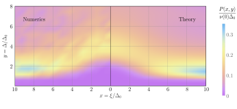
Figure 4: A color map of the joint probability density function $P\left(x,y\right)$ of the onsite values of dimensionless disorder field $x=\xi/\Delta_{0}$ and dimensionless order parameter $y=\Delta/\Delta_{0}$ in the vicinity of the Fermi surface corresponding to $\xi=0$. The color encodes the value of the probability density according to the legend to the right. The left color map corresponds to (smoothened) histogram obtained from direct numerical solution of the original self-consistency equations (LABEL:saddle-point_order-parameter), and the right color map reflects the result of the theoretical calculation performed according to expression (LABEL:joint-distribution_expression-via-m) with the $m$ function determined from the numerical solution of equations (24-25). For simplicity, the model with $D\left(\xi\right)=\text{const}$ is used. The parameters of the model in both cases are $\lambda\approx 0.120$ and $Z=51$, which corresponds to $\kappa=5.0$. The observed jitter in the results of the direct numerical solution (left plot) is due to the finite size of the corresponding sample: even despite the fact that a system with $N=2^{22}\approx 4.2\cdot 10^{6}$ sites is used, only $\sim N\cdot\left(2\nu_{0}\Delta_{0}\right)\sim 6\cdot 10^{4}$ of them contribute to the presented histogram, resulting in an average of just $\sim 250$ points contributing to each bin of the histogram for the chosen bin size $\Delta x=\Delta y\approx 0.71$. The two color maps demonstrate reasonable agreement, simultaneously reproducing several important qualitative features of the joint PDF. In particular, one observes a considerable deformation of the conditional distribution $P_{\text{c}}\left(\Delta\right):=P\left(\xi,\Delta\right)/P\left(\xi\right)$ as $\left|\xi\right|$ decreases. See the Main Text for a detailed discussion.

While the distribution quickly approaches the profile corresponding to the factorized distribution of the form $P_{0}\left(y\right)\cdot P\left(x\right)$ at sufficiently large values of $\xi$, there is a noticeable deformation in the region $\xi/\Delta_{0}\apprle 5$ indicative of the strong correlation between the onsite values of $\xi$ and $\Delta$. As can be seen from the original self-consistency equation (LABEL:saddle-point_order-parameter), such behavior is a secondary consequence of the fact that a low value of $\xi$ at a given site $i$ results in an increase of the order parameter at all neighboring sites $j\in\partial i$ by a contribution of the order $D\left(\xi_{j}\right)/Z\sim\Delta_{0}\cdot\kappa$. This, in turn, leads to the enhancement of the value of the order parameter on the chosen site $i$. These qualitative considerations allow one to estimate the position of the conditional distribution average $\Delta_{\text{av}}\left(\xi\right)=\intop d\Delta\cdot\Delta\cdot P\left(\Delta,\xi\right)/P\left(\xi\right)$ as an appropriate solution to the following system of equations:

$$\Delta_{\text{av}}\approx\Delta_{\text{neighb}}\left(1+\lambda\cdot\ln\frac{\left\langle\Delta\right\rangle}{\Delta_{\text{neighb}}}\right),$$ (59)

$$\Delta_{\text{neighb}}\approx\left\langle\Delta\right\rangle+\kappa\Delta_{0}\cdot\frac{\Delta_{\text{av}}}{\sqrt{\Delta_{\text{av}}^{2}+\xi^{2}}}.$$ (60)

At large values of $\xi$ the solution $\Delta_{\text{av}}$ approaches the total expectation $\left\langle\Delta\right\rangle$, while at $\xi\rightarrow 0$ the result behaves as $\Delta_{\text{av}}\approx\left\langle\Delta\right\rangle+\kappa\Delta_{0}$, in full agreement to what is observed on 4. A plot of the full dependence $\Delta_{\text{av}}\left(\xi\right)$ is presented on 5 and shows a reasonable agreement with both data obtained from the direct numerical solutions of the self-consistency equations and the curve calculated by appropriate numerical integration of the theoretical expression (LABEL:joint-distribution_expression-via-m).

Figure 5: The plot of the conditional average of the dimensionless order parameter $\Delta_{\text{av}}\left(\xi\right)/\Delta_{0}=\intop d\Delta\cdot\Delta/\Delta_{0}\cdot P\left(\Delta,\xi\right)/P\left(\xi\right)$ as a function of onsite value of the dimensionless disorder field $x=\xi/\Delta_{0}$. The blue points corresponds to the result calculated from the direct numerical solution of the self-consistency equations (LABEL:saddle-point_order-parameter). The solid green line corresponds to the conditional average computed by direct integration from the theoretical joint probability distribution given by Eq. (LABEL:joint-distribution_expression-via-m), with the $m$ function determined from the numerical solution of equations (24-25). The red dashed line corresponds to physically relevant solution of the approximate equations (59-60). Finally, the black dashed line denotes the value of the total average $\left\langle\Delta\right\rangle/\Delta_{0}$ of the dimensionless order parameter as found from both the numerical data and analytic theory. The microscopic parameters of the model are $D\left(\xi\right)=\text{const}$, $\lambda\approx 0.120$, $Z=51$ and $\kappa=5.0$, so that a direct comparison with 4 is appropriate.

We would like to emphasize, however, that this behavior is subject to revision upon introduction of the Onsager reaction term discussed in II.3. While we expect that for $Z\geq Z_{1}$ this term is of little importance for the distribution function of the order parameter, the profile of the onsite joint distribution function $P\left(\Delta,\xi\right)$ at $\left|\xi\right|\sim\Delta$ can potentially experience noticeable deformations from the described behavior. Indeed, the physical interpretation of the reaction term is to mediate the self-action of the order parameter, that is, the indirect response of a given quantity to its own change through the corresponding responses of the neighboring fields. The latter mechanism is precisely what leads to the described profile of the joint probability function at small values of $\left|\xi\right|$. That is why even for sufficiently large values of $Z$ the Onsager reaction term might have a significant effect on the shape of the onsite joint distribution function $P\left(\Delta,\xi\right)$ for $\left|\xi\right|\sim\Delta$.

It is also worth mentioning that the joint probability distribution $P\left(\Delta,\xi\right)$ is of more physical significance than the distribution $P\left(\Delta\right)$ of the order parameter alone. Indeed, computation of various physical observables for the given configuration of the order parameter involves values both $\xi$ and $\Delta$ for states close to Fermi level, i. e. with $\left|\xi\right|\sim\Delta$. As Figures 4 and 5 suggest, treating fields $\xi$ and $\Delta$ as independent would thus result in qualitatively incorrect results. One particular example of this is the spectrum of collective low-energy excitations discussed in Ref. (Feigelman_Microwave_2018, ): the inverse Green’s Function of those modes is sensitive to onsite values of $\xi$ and $\Delta$ in equal measures, so that computing the average Green’s Function actually demands the aforementioned joint distribution close to the Fermi surface. Another important question yet to be analyzed is the connection between the field of the order parameter $\Delta$ discussed in this work and experimentally measurable quantities. While the order parameter in weakly disorder superconductors can be probed e.g. via the single-particle density of states (L0_1972, ), no theory exists to our knowledge of a similar connection in the case of strong disorder with a pseudogap. We believe such a theory will inevitably require the knowledge of joint distribution functions of both $\xi$ and $\Delta$.

III.7 The effect of weak fluctuations of the coupling amplitudes

In this Subsection, we analyze a generalization of our model that allows for the fluctuations of the interaction matrix element between each pair of interacting single-particle states. We model these fluctuations by assigning a random magnitude to the bare matrix element $D_{ij}$ of the interaction between each pair of interacting states on top of its smooth dependence on the energy difference $\xi_{i}-\xi_{j}$ of the two states. This corresponds to the following generalization of the self-consistency equation (LABEL:saddle-point_order-parameter):

$$\Delta_{i}=\sum_{j\in\partial i}c_{ij}D\left(\xi_{i}-\xi_{j}\right)\frac{\Delta_{j}}{\sqrt{\Delta_{j}^{2}+\xi_{j}^{2}}},$$ (61)

where $D\left(\xi\right)$ is the energy dependence of the interaction described previously, and $c_{ij}$ are independent random variables distributed according to some distribution $P\left(c\right)$. In particular, letting $P\left(c\right)=\delta\left(c-1\right)$ leads one back to the self-consistency equation (LABEL:saddle-point_order-parameter) analyzed earlier. The new equation (LABEL:fluctuating-coupling_saddle-point-equation) now includes two sources of disorder: the randomness of the single-particle energies $\xi_{i}$ and the one from the distribution of the coupling matrix elements $D_{ij}=c_{ij}\cdot D\left(\xi_{i}-\xi_{j}\right)$.

One can conduct the mean-field analysis of Eq. (LABEL:fluctuating-coupling_saddle-point-equation) similar to that of II.4. The latter is still valid for sufficiently large number of neighbors, i. e. $\left\langle c\right\rangle Z\cdot 2\nu_{0}\Delta\gg 1$. One can then assert a spatially uniform order parameter for energies close to the to Fermi surface and obtain

$$\Delta_{R}=2E_{0}\cdot\exp\left\{-\frac{1}{\lambda_{R}}\right\},\,\,\,\,\,\,\lambda_{R}=\left\langle c\right\rangle 2\nu_{0}D\left(0\right)Z,$$ (62)

where $\lambda_{R}$ is the new dimensionless Cooper attraction constant, and the value of $E_{0}\sim\varepsilon_{D}$ is still determined by higher energy scales, but with the new value of the mean matrix element.

Our theoretical approach can be generalized to describe the model above, as explained in detail in G. In particular, the $m$ function retains its role of the central object in the theory. Here, we only present the proper counterpart of Eq.-s (24-25) valid for $x\apprle\varepsilon_{D}/\Delta_{0}$:

$$m_{1}\left(w\right) =m_{1}\left(0\right)+\boxed{\left\langle c^{2}\right\rangle}\cdot\kappa w\alpha+\boxed{\left\langle c\right\rangle}\cdot\lambda\intop_{0}^{1}dw_{1}\cdot\sqrt{1-w_{1}^{2}}\cdot\frac{m_{1}\left(w_{1},0\right)-m_{1}\left(0,0\right)}{w_{1}}$$

$$+\lambda\intop_{0}^{\infty}dy_{1}\cdot y_{1}\ln\frac{1}{y_{1}}\cdot\intop_{\mathbb{R}-i0}\frac{ds}{2\pi}\cdot\boxed{\intop dcP\left(c\right)}\cdot\boxed{c}\exp\left\{i\boxed{c}s\kappa w\right\}\cdot\exp\left\{m\left(s|0,0\right)-isy_{1}\right\},$$ (63)

$$m_{2}\left(S|w\right)=\lambda\cdot\boxed{\intop dcP\left(c\right)}\cdot\intop_{0}^{1}dw_{1}\cdot\frac{\exp\left\{iS\kappa\boxed{c}w_{1}\right\}-1-iS\kappa\boxed{c}w_{1}}{w_{1}^{2}\sqrt{1-w_{1}^{2}}}\cdot\left[1-w_{1}\left(1-w_{1}^{2}\right)\frac{\partial}{\partial w_{1}}\right]\cdot\left[\frac{\boxed{c}\kappa w+m_{1}\left(w_{1}\right)}{\kappa}\right].$$ (64)

In these equations, the boxes highlight the difference brought in by the fluctuations of the matrix element in comparison with equations (24-25). Once the solution to these equations is found, expressions (LABEL:joint-distribution_expression-via-m) and (LABEL:expr-for-P0-via-m) for the probability density of the dimensionless order parameter $P_{0}\left(y\right)$ and the joint probability density $P\left(x,y\right)$ of onsite values of $x=\xi_{i}/\Delta_{0}$ and $y=\Delta_{i}/\Delta_{0}$ are applicable without modifications.

III.7.1 Generalization to fluctuating number of neighbors $Z$

We first note that these equations allow one to effortlessly analyze the effect of the fluctuating number of neighbors $Z$. To this end, one lets $P\left(c\right)=p\cdot\delta\left(1-c\right)+\left(1-p\right)\delta\left(c\right)$, so that each edge is either “turned on” with probability $p\in\left[0,1\right]$, or “turned off” with probability $1-p$. As a result, each site has a fluctuating number of neighbors with Poisson distribution characterized by mean value $\left\langle Z\right\rangle=pZ$. With such choice of the distribution function $P\left(c\right)$ one can explicitly perform all the averages in Eq.-s (63-64). Remarkably, the outcome is identical to the equations (24-25) for the case without fluctuations of the number of neighbors upon proper renormalization of the microscopical constants $\lambda,\alpha,Z,\Delta_{0},\kappa$. Namely, one simply has to replace

$$\lambda\mapsto\lambda_{R}=p\lambda,\,\,\,\alpha\mapsto\alpha_{R}=p\alpha$$ (65)

and calculate all other low-energy quantities in the theory using these modified values. One particular example of this is the mean-field value of the order parameter (LABEL:fluctuating-coupling_mean-field) that now contains precisely $\lambda_{R}$ in both the exponent and the prefactor $E_{0}$ defined by higher energies. Consequently, the remaining microscopical constants are renormalized as

$$Z_{R}=pZ,\,\,\,\kappa_{R}=\frac{\lambda_{R}}{\Delta_{R}\cdot Z_{R}}.$$ (66)

The derivation of these results is presented in G.5. We once again underscore that such a picture implies absence of any practical significance of the fluctuations of the number of neighbors in our model.

III.7.2 Weak fluctuations of the coupling constant $\lambda$

A more complicated situation arises, however, if one introduces disorder in the value of $c$ itself. For this calculation, we choose $c$ to be distributed according to a narrow distribution with mean value $\left\langle c\right\rangle=1$, variance $\left\langle\left(c-1\right)^{2}\right\rangle=\delta^{2}$ and exponentially decaying tails. One can then repeat the asymptotic analysis of III.4 to extract the influence of the introduced fluctuations of the coupling matrix elements on the extreme value statistics. A detailed exposition is presented in G, while here we summarize the key results and qualitative conclusions.

In the region of small value of $y$, that corresponds to a unique saddle point of the form $S=+it,\,\,t\gg 1$, one can expand the Eq. (LABEL:fluctuating-coupling_m1-equation) w.r.t small deviations of $c$ from its mean value. Upon estimating the probability (LABEL:expr-for-P0-via-m) with the help of the resulting asymptotic expression, the double-exponential asymptotic behavior described by Eq.-s (46-47) remains valid with only a slight modification of the form

$$\zeta\left(y\right)\mapsto\zeta\left(y\right)\exp\left\{\delta^{2}/2\right\}.$$ (67)

However, with finite $\delta$ this regime now extends only to a finite lower value of the probability density:

$$P_{0}\left(y\right)\apprge\frac{1}{\sqrt{2\pi\cdot\lambda\left\langle y\right\rangle\kappa\delta^{2}}}\exp\left\{-\frac{\lambda\left\langle y\right\rangle}{\kappa\delta^{2}}\right\}.$$ (68)

This also implies that the double-exponential regime is only present while

$$\delta\apprle\sqrt{\lambda/\kappa}=\sqrt{Z_{\text{eff}}}.$$ (69)

The value of $P_{0}\left(y\right)$ for larger values of $\delta$ is described by a different asymptotic behavior with much slower decay in the region of small $y/\left\langle y\right\rangle$. It can be interpreted as a change in the type of the dominating optimal fluctuation that delivers the body of the distribution for low values of the order parameter. Indeed, for the case with $\delta=0$ the only way to render a small value of the order parameter was to have all neighboring values of $\left|\xi\right|$ large enough, as explained in III.4. However, sufficiently strong fluctuations of the coupling constant provide a finite probability of a region with a diminished values of the coupling constant to neighboring sites with relatively small values of $\xi$. The behavior of the distribution would thus reflect the competition between these two sets of configurations. As a consequence, one expects that in this case the answer will be sensitive to the particular form of the distribution $P\left(c\right)$ as well as any local correlations present in the joint distribution of the coupling matrix elements $c_{ij}$ and the onsite energies $\xi_{i}$.

The asymptotic behavior of the distribution for large values of the order parameter can also be analyzed within the perturbative expansion of Eq. (LABEL:fluctuating-coupling_m1-equation) w.r.t small deviation of $c$ from its mean value. One obtains that each of the multiple saddles point of the integral (LABEL:expr-for-P0-via-m) for the probability acquire an additional multiplier that can be estimated as

$$P_{0}^{\left(n\right)}\left(y\right)\sim P_{0}^{\left(n\right)}\left(y,\delta=0\right)\cdot\exp\left\{\frac{\left(z_{n}\delta\right)^{2}}{2}\frac{y-\left\langle y\right\rangle}{\kappa}\right\},$$ (70)

where $z_{n}=iS_{n}\kappa$ describes the position of the corresponding saddle point, and $P_{n}\left(y,\delta=0\right)$ stands for the magnitude of the contribution without fluctuations of the matrix element. This result implies that the asymptotic expression (LABEL:P0-large-y-tail) delivered by the main saddle point with $n=0$ remains qualitatively intact up to $\delta\sim 1$, at which point the perturbative expansion w.r.t small $\delta$ ceases to be applicable. Furthermore, each secondary saddle point acquires an extra multiplier of the form $\exp\left\{-\frac{\left(2\pi n\delta\right)^{2}}{2}\frac{y-\left\langle y\right\rangle}{\kappa}\right\}$ due to the imaginary part $z_{n}$ which is close to $2\pi n$. As a result, the oscillations produced by these secondary saddle points are suppressed at $2\pi\delta\sim 1$.

6 below presents the demonstration of the qualitative picture presented above in the form of both theoretical curves and histograms obtained from direct numerical solution of the modified self-consistency equations (LABEL:fluctuating-coupling_saddle-point-equation) for several realizations of the disorder. In particular, it clearly illustrates the persistence of both asymptotic trends observed in III.4, while also demonstrating how the secondary maxima are smeared as the value of $\delta$ is growing.

Figure 6: A log-scale plot for the PDF of the dimensionless order parameter $P\left(\Delta/\Delta_{0}\right)$ for various strength of the fluctuations of the interaction matrix element $D_{ij}=c_{ij}D\left(\xi_{i}-\xi_{j}\right)$. The distribution of $c$ is log-normal with parameters that ensure $\left\langle c\right\rangle=1$, $\left\langle\left(c-1\right)^{2}\right\rangle=\delta^{2}$. The solid lines represent the smoothened histogram obtained from direct numerical solution of the self-consistency equations (LABEL:fluctuating-coupling_saddle-point-equation) on 3 instances of Random Regular Graph of size $N=2^{17}\approx 1,3\cdot 10^{5}$. The dashed lines uses the proper generalization of the weak coupling approximations of III.3 to approximate the value of the $m$ function used to compute the integral (LABEL:expr-for-P0-via-m) for the PDF. Finally, the dashed red line corresponds to approximate analytic expressions for the case without fluctuations of coupling matrix element: Eq. (LABEL:P0-large-y-tail) for large values of $y>\left\langle y\right\rangle$ and Eq.-s (46-47) for $y<\left\langle y\right\rangle$. The microscopic parameters of the model are $D\left(\xi\right)=\text{const}$, $\lambda\approx 0.120$, $Z=51$ and $\kappa=5.0$. The mismatch between the theoretical description and the numerical histogram originates from subleading corrections of order $O\left(\Delta_{0}/\lambda\right)$ and $O\left(\lambda^{2}\right)$, see also notes on this under 2

IV Discussion and Conclusions

In the present paper we developed systematic theory able to describe statistics of superconducting order parameter in strongly disordered pseudo-gaped superconductors. We have discovered the existence of a wide region of parameters where usual semiclassical approach to dirty superconductors is not valid, but, at the same time, the universal behavior typical for the close proximity to SIT (Feigelman_SIT_2010, ) does not take place either. In this wide range of parameters, the shape of the distribution function $P\left(\Delta\right)$ is controlled by the single parameter $\kappa$ defined in Eq. (LABEL:Z-eff_and_kappa_definition). Small $\kappa$ corresponds to limit of weak disorder that is typical for usual dirty superconductors. This limit is characterized by narrow Gaussian distribution of the order parameter is observed, see Eq. (LABEL:P0-Gaussian-regime). On the other hand, at $\kappa\apprge\lambda$, with $\lambda$ being the dimensionless Cooper constant, the distribution becomes highly non-trivial. We are able to calculate its explicit form for all values of $\Delta/\Delta_{0}$ in terms of certain special functions, as presented in III.3. The asymptotic behavior of the distribution density $P\left(\Delta\right)$ is given by equations (46-47) and (LABEL:P0-large-y-tail) for small and large values of $\Delta/\Delta_{0}$ respectively. These functions do depend on the value of $\kappa$; in principle, it opens the possibility to extract the value of $\kappa$ for specific disordered superconductor via measuring the local distribution $P\left(\Delta\right)$ by means of scanning tunneling methods. Our model, however, breaks down in a small vicinity of the SIT described by exponentially large values of $\kappa\apprge\exp\left\{\frac{1}{2\lambda}\right\}\gg 1$. The phase diagram following from our findings is sketched on 7.

Figure 7: Qualitative phase diagram describing the behavior of the distribution of the order parameter $P\left(\Delta\right)$ in strongly disordered superconductors. The horizontal axis schematically describes the strength of disorder measured by the parameter $\kappa$ defined in Eq. (LABEL:Z-eff_and_kappa_definition). Various colors indicate the perceived level of inhomogeneity of the superconducting state: the green color corresponds to a well pronounced superconducting state with nearly uniform value of the order parameter, light-green and white colors represent a manifestly nonuniform superconducting state with strongly non-Gaussian or even critical distributions of the order parameter, and the red color stands for the insulating state of the system with no superconducting order parameter. The blue dashed line highlights the range of parameters available to our theoretical description.

We emphasize that the very existence of a separate region with a broad range of disorder strengths featuring a non-trivial profile of the distribution function $P\left(\Delta\right)$ is related to the smallness of Cooper attraction constant $\lambda\ll 1$. Until recently, small-$\lambda$ region was not attainable for direct numerical simulations of real 2D and 3D systems due to size restrictions. Advances in this field (Evers2019, ; PhysRevB.102.184507, ; Trivedi2021, ) seem to make such a study possible.

The shape of distribution function $P\left(\Delta\right)$ was found to differ considerably from the fat-tail distributions obtained previously in Ref.-s (Feigelman_SIT_2010, ; Lemarie2013, ) by different analytic and numerical methods. Concerning available experimental data, we note, first of all, that the interpretation of the tunneling conductance $dI/dV$ in terms of the theoretical order parameter is not straightforward in the case of large spatial fluctuations $\Delta\left(\boldsymbol{r}\right)$. Indeed, in such case the half-width of the gap defined as the energy distance between the peaks in $dI/dV$ is not just given by the order parameter $\Delta$ itself, as it is the case in the classical superconductor with constant $\Delta$. In fact the shape of $dI/dV$ is controlled by the local Density of States (DoS) $\nu\left(E\right)$ which should be obtained, in principle, via the solution of the generalized Usadel equation for the local electron Green function in the background of spatially fluctuating order parameter $\Delta\left(\boldsymbol{r}\right)$ as well as in presence of a pseudo-gap. Such a program had never been implemented yet, to our knowledge.

Qualitatively, it seems evident that more direct access to the local values of $\Delta\left(\boldsymbol{r}\right)$ is provided by the heights $R$ of the "coherence peaks" in local tunneling conductance $dI/dV\left(\boldsymbol{r}\right)$. Early experimental data (Sacepe_2011_for-pair-preformation, ) demonstrates substantial change in the distribution of peak heights $\mathcal{P}\left(R\right)$ with the increase of disorder, similarly to the effect of increasing our theoretical parameter $\kappa$ upon the shape of $P_{0}\left(\Delta\right)$, see 2. Another type of theoretical analysis provided in Ref. (Lemarie2013, ) predicts extremely broad distribution of the Tracy-Widom universal shape in terms of the logarithmic variable $R_{s}=\ln R/\left\langle R\right\rangle$; however, their experimental data on Fig. 6 leaves space for different interpretations as well. A recent study (PhysRevB.102.184507, ) of strongly disordered 3D superconductor by means of numerical solution of Bogolyubov-De Gennes equations provides a number of various distribution functions for $P\left(\Delta\right)$, which could be analyzed in terms of our theory; for now we can say that the generic feature — an increase of normalized width of the distribution with disorder — is reproduced there as well.

The model we have studied here is limited in several regards. First of all, our initial model approximates the matrix element of the Cooper attraction by a constant value, that is further endowed with a weak dependence energy difference. However, the actual amplitude of the interaction in each disorder realization is proportional with the overlap of the corresponding wave-functions $\intop\psi_{i}^{2}\left(\boldsymbol{r}\right)\psi_{j}^{2}\left(\boldsymbol{r}\right)d\boldsymbol{r}$ and thus exhibits direct statistical fluctuations at least of the order of its mean value. In III.7 we have briefly analyzed an extended model that incorporates this effect in the simplest fashion possible. Our analysis indicates that these direct statistical fluctuations do not alter our conclusions about the large-value asymptotic behavior of the distribution of the order parameter, while only removing several unphysical features such as secondary maxima. However, it also follows from our results that even relatively small fluctuations of the interaction matrix element can distort the low-value asymptotic behavior of the distribution of the order parameter. The character of this distortion is generally sensitive to the local structure of the distribution of the matrix elements and requires further analysis.

Secondly, the energy dependence of the matrix element $D\left(\omega=\left|\xi_{i}-\xi_{j}\right|\right)$ is assumed to be smooth at the relevant energy scale of Debye energy $\varepsilon_{D}$. It is not necessarily the case for strongly disordered superconductor with the Fermi energy located inside the localized band; the point is that the relevant matrix elements between localized eigenstates contain (Feigelman_Fractal-SC_2010, , Subsec. 2.2.5) the Mott resonances leading to a singular behavior $D\left(\omega\right)\propto\left|\ln\omega/\delta_{L}\right|^{d-1}$. This feature can be incorporated in our approach as long as the overall separation of scales $\Delta\ll\varepsilon_{D},E_{F}$ is maintained.

Thirdly, we have analyzed the mean-field equations for $T=0$ only. Non-zero temperatures can be included into our formalism simply by multiplying the function $f\left(\xi_{j},\Delta_{j}|\xi_{i}\right)$ defined in Eq. (LABEL:saddle-point-rhs_notation) by $\tanh\frac{\sqrt{\Delta_{j}^{2}+\xi_{j}^{2}}}{2T}$. It will complicate further analysis, but low-$T$ corrections to the obtained results are possible to derive.

The nearest extensions of the developed theory will contain study of low-energy collective modes in strongly disordered superconductors. The aim is to revisit this subject, considered originally in Ref. (Feigelman_Microwave_2018, ) with the presently developed understanding about the order parameter distribution. Another important subject is to include the Onsager reaction term in our free energy functional; it would allow to consider the region closer to SIT by our methods. Finally, it is of practical importance to establish a reliable connection between the order parameter $\Delta$ studied in this work and experimentally measurable quantities, as none such connections exist to date for strongly disordered superconductors.

eqapp refcmd=(LABEL:#1) eq refcmd=(LABEL:#1) of the Main Text app refcmd=Section LABEL:#1 subsecapp refcmd=Subsection LABEL:#1 subsec refcmd=Subsection LABEL:#1 of the Main Text sec refcmd=Section LABEL:#1 of the Main Text figapp refcmd=Figure LABEL:#1 fig refcmd=Figure LABEL:#1 of the Main Text

Supplementary Material A The Saddle-point Approximation

In this Appendix, we present a concise description of the saddle-point approximation for the model Hamiltonian (LABEL:Model-Hamiltonian). The partition function $\mathcal{Z}$ and the free energy $F$ of the model are defined as

$$-\beta F=\ln\mathcal{Z}=\ln\text{Tr}\left\{\exp\left\{-\beta H\right\}\right\},$$ (71)

where the trace is taken over all fermionic degrees of freedom that correspond to eigenstates of Cooper pair occupation operator:

$$n_{i}=\frac{1}{2}\left(a_{i\downarrow}^{\dagger}a_{i\downarrow}+a_{i\uparrow}^{\dagger}a_{i\uparrow}\right)=\left\{0,1\right\}.$$ (72)

This limitation arises due to the presence of a large pseudogap in the system, see II.1 for more details.

A.1 Saddle point free energy

It is convenient to rewrite the partition function 71 in terms of imaginary time interaction picture with respect to the non-interacting part of the Hamiltonian. The latter is defined as

$$H_{0}:=\sum_{i}\xi_{i}\left(a_{i\downarrow}^{\dagger}a_{i\downarrow}+a_{i\uparrow}^{\dagger}a_{i\uparrow}\right).$$ (73)

Time-dependent operators in the interaction picture then reads

$$X\left(\tau\right)=e^{\tau H_{0}}Xe^{-\tau H_{0}}.$$

One can then represent the partition function in the following way:

$$-\beta F=\ln\text{Tr}\left\{\text{Texp}\left\{-\beta H_{\text{int}}\left(\tau\right)\right\}e^{-\beta H_{0}}\right\}.$$ (74)

Here, the symbol Texp stands for the imaginary-time-ordered exponent, and $H_{\text{int}}$ is the interaction term:

$$H_{\text{int}}\left(\tau\right)=-\sum_{\left\langle ij\right\rangle}D\left(\xi_{i}-\xi_{j}\right)\left(a_{i\downarrow}^{\dagger}\left(\tau\right)a_{i\uparrow}^{\dagger}\left(\tau\right)a_{j\uparrow}\left(\tau\right)a_{j\downarrow}\left(\tau\right)+\text{Herm. conj.}\right).$$ (75)

Under the sign of the time ordering, one can decouple the interaction term by means of the functional Hubbard-Stratanovich transformation [38]:

$$\text{Texp}\left\{-\beta H_{\text{int}}\left(\tau\right)\right\}=\frac{1}{\mathcal{Z}_{\Delta}}\intop_{\Delta\left(0\right)=\Delta\left(\tau\right)}D\Delta\left(\tau\right)\cdot\exp\left\{-S_{\Delta}\left[\Delta\right]\right\}\cdot\text{Texp}\left\{+\sum_{i}\intop d\tau\left(a_{i\downarrow}^{\dagger}\left(\tau\right)a_{i\uparrow}^{\dagger}\left(\tau\right)\Delta_{i}\left(\tau\right)+\text{Herm. conj.}\right)\right\},$$ (76)

$$\mathcal{Z}_{\Delta}=\intop_{\Delta\left(0\right)=\Delta\left(\tau\right)}D\Delta\left(\tau\right)\cdot\exp\left\{-S_{\Delta}\left[\Delta\right]\right\},$$ (77)

where the functional integration is done over all complex fields $\Delta_{i}\left(\tau\right)$ obeying periodic boundary conditions w.r.t $\tau$. The integration weight is given by the following imaginary time action:

$$S_{\Delta}=\frac{1}{2}\sum_{ij}\cdot\intop_{0}^{\beta}d\tau\cdot\Delta_{i}^{*}\left(\tau\right)\cdot\left(V^{-1}\right)_{ij}\cdot\Delta_{j}\left(\tau\right),$$ (78)

where $V^{-1}$ is the matrix inverse to the interaction matrix element, viz.

$$\sum_{j:\left\langle jk\right\rangle}\left(V^{-1}\right)_{ij}\cdot D\left(\xi_{i}-\xi_{k}\right)=\delta_{ik}.$$ (79)

One typically expects the mean field analysis to be perfectly applicable for a well developed superconductivity away from the transition temperature, i. e. for $1-T/T_{c}\gg\text{Gi}$. For the functional representation 76, this corresponds to evaluating the functional integral by means of the saddle-point approximation. The saddle-point configuration of the order parameter is time-independent, so that the saddle-point value of the free energy corresponds to the minimum of the following free energy function with respect to the order parameter:

$$-\beta F\left[\Delta\right]=-\frac{\beta}{2}\sum_{ij}\cdot\Delta_{i}^{*}\cdot\left(V^{-1}\right)_{ij}\cdot\Delta_{j}+\ln\text{Tr}\left\{\exp\left\{-\beta H_{\text{MF}}\right\}\right\},$$ (80)

$$H_{\text{MF}}=\sum_{i}\xi_{i}\left(a_{i\downarrow}^{\dagger}a_{i\downarrow}+a_{i\uparrow}^{\dagger}a_{i\uparrow}\right)-\sum_{i}\left(\Delta_{i}a_{i\downarrow}^{\dagger}a_{i\uparrow}^{\dagger}+\text{Herm. conj.}\right).$$ (81)

The second term in 80 is obtained after using the fact that for the case of time-independent $\Delta$ field, the trace of the time-ordered exponent can be rewritten in terms of a trace over fermionic degrees of freedom of the mean field Hamiltonian $H_{\text{MF}}$.

The second term in 80 can be evaluated explicitly:

$$\ln\text{Tr}\left\{\exp\left\{-\beta H_{\text{MF}}\right\}\right\}=\sum_{i}\ln\left[2e^{-\beta\xi_{i}}\cosh\left\{\beta\sqrt{\xi_{i}^{2}+\left|\Delta_{i}\right|^{2}}\right\}\right].$$ (82)

Note that this expression differs from a similar term in the conventional theory of superconductivity by absence of the quasi-particle contribution, as the latter is exponentially suppressed due to the well-developed pseudogap. The final expression for the free energy then reads:

$$F\left[\Delta\right]=\frac{1}{2}\sum_{ij}\cdot\Delta_{i}^{*}\cdot\left(V^{-1}\right)_{ij}\cdot\Delta_{j}-T\sum_{i}\ln\left[2\cosh\left\{\beta\sqrt{\xi_{i}^{2}+\left|\Delta_{i}\right|^{2}}\right\}\right]+\sum_{i}\xi_{i}.$$ (83)

A.2 Saddle point equation for the order parameter

The order parameter is determined as the minimum of the saddle-point free energy 83. The corresponding saddle point equation reads:

$$\frac{\partial F\left[\Delta\right]}{\partial\Delta_{i}^{*}}=0\Leftrightarrow\sum_{j}\cdot\left(V^{-1}\right)_{ij}\cdot\Delta_{j}-\frac{\Delta_{i}}{\sqrt{\left|\Delta_{i}\right|^{2}+\xi_{i}^{2}}}\cdot\tanh\left\{\beta\sqrt{\xi_{i}^{2}+\left|\Delta_{i}\right|^{2}}\right\}.$$ (84)

Reverting back the $V$ matrix renders the celebrated self-consistency equation:

$$\Delta_{i}=\sum_{j\in\partial i}f\left(\xi_{j},\Delta_{j}|\xi_{i}\right),$$ (85)

$$f\left(\xi,\Delta|\xi_{0}\right)=D\left(\xi-\xi_{0}\right)\frac{\Delta}{\sqrt{\left|\Delta\right|^{2}+\xi^{2}}}\tanh\left\{\beta\sqrt{\left|\Delta\right|^{2}+\xi^{2}}\right\}.$$ (86)

In the absence of magnetic field and similar time-reversal symmetry breaking factors, the order parameter can be chosen to be real and positive. Finally, the zero temperature case corresponds to $\beta\rightarrow\infty$, which results in the equation (LABEL:saddle-point_order-parameter):

$$\Delta_{i}=\sum_{j\in\partial i}D\left(\xi_{j}-\xi_{i}\right)\frac{\Delta_{j}}{\sqrt{\Delta_{j}^{2}+\xi_{j}^{2}}}.$$ (87)

A.3 Mean field solution at zero temperature

It is informative to analyze the resulting self-consistency equation 87 in the regime of weak disorder, when the order parameter is nearly homogeneous. As already discussed in II.4, this approach is justified for sufficiently large number of neighbors $Z$ by virtue of the central limit theorem. In this case, one can simplify the self-consistency equation at zero temperature 87 to the following form:

$$\Delta\left(\xi_{0}\right)=Z\cdot\intop d\xi\cdot\nu\left(\xi\right)\cdot D\left(\xi-\xi_{0}\right)\frac{\Delta\left(\xi\right)}{\sqrt{\Delta^{2}\left(\xi\right)+\xi^{2}}}.$$ (88)

This expression represents an integral equation on the value of the order parameter $\Delta$ for a site with a given value of the onsite disorder $\xi_{0}$.

Let us now take into account that the $D$ function describes some weak attraction with a typical energy scale being the Debye energy $\varepsilon_{D}$. Similarly to the conventional theory of superconductivity, the resulting value of the order parameter then appears to be exponentially small with respect to the dimensionless coupling constant. For our model, the latter is defined is

$$\lambda=2\nu_{0}\cdot ZD\left(0\right).$$ (89)

The exponential smallness then follows from the fact that the integral over $\xi$ in the right hand side of 88 is logarithmic due to the $1/\xi$ asymptotic of the expression with a square root. Secondly, because the superconducting scale $\Delta$ is exponentially smaller than the Debye energy $\varepsilon_{D}$, the key role of $D\left(\xi\right)$ is to provide an upper cut-off for the otherwise logarithmically diverging integral over $\xi$ in 88. The integral itself can thus be estimated as:

$$\intop d\xi\cdot\nu\left(\xi\right)\cdot D\left(\xi-\xi_{0}\right)\frac{\Delta\left(\xi\right)}{\sqrt{\Delta^{2}\left(\xi\right)+\xi^{2}}}\sim 2\nu\left(0\right)\cdot D\left(0\right)\ln\frac{\varepsilon_{D}}{\Delta\left(0\right)}+\text{const},$$

where the constant term of order unity is controlled by high energies, as we will demonstrate below. This also implies that the $\xi_{0}$-dependence of the order parameter approximately replicates that of $D\left(\xi_{0}\right)$, thus also suggesting the scale of order $\xi_{0}\sim\varepsilon_{D}$ for the dependence of $\Delta$ on $\xi_{0}$.

To conduct a more quantitative analysis, let us introduce the following notation:

$$u\left(\xi\right):=\frac{D\left(\xi\right)}{D\left(0\right)},\,\,\,\,\,d\left(\xi_{0}\right):=\frac{\Delta\left(\xi_{0}\right)}{\Delta_{0}},\,\,\,\,\,\Delta\left(0\right)=\Delta_{0},\,\,\,\,\,\nu_{0}=\nu\left(0\right).$$ (90)

As discussed above, both $u\left(\xi\right)$ and $d\left(\xi_{0}\right)$ are expected to have $\varepsilon_{D}$ as the energy scale of the $\xi$-dependence. Note also that both $u$ and $d$ functions are normalized as $u\left(0\right)=d\left(0\right)=1$ by construction. In this notation, the mean field equation 88 reads

$$d\left(\xi_{0}\right)=\lambda\cdot\intop d\xi\cdot\frac{\nu\left(\xi\right)}{2\nu_{0}}\cdot u\left(\xi-\xi_{0}\right)\frac{d\left(\xi\right)}{\sqrt{\Delta_{0}^{2}\cdot d^{2}\left(\xi\right)+\xi^{2}}}.$$

Assuming that the value of $\Delta_{0}$ is the smallest energy scale in the problem, one can perform two important simplifications. First, one neglects the $\xi$-dependence of the expression under the square root, as it rendered irrelevant already for $\left|\xi\right|\apprge\Delta_{0}$, well below the region where $u\left(\xi\right)$ deviates from unity considerably. Secondly, one can split the integral over $\xi$ into two contributions: the low energy part gaining its value at $\left|\xi\right|\sim\Delta_{0}$ and the high-energy part collecting its value from a large region $\Delta_{0}\ll\left|\xi\right|\apprle\varepsilon_{D}$. The result reads:

$$d\left(\xi_{0}\right) =\lambda\cdot\intop d\xi\cdot\frac{\nu\left(\xi\right)}{2\nu_{0}}\cdot u\left(\xi-\xi_{0}\right)\frac{d\left(\xi\right)}{\sqrt{\Delta_{0}^{2}+\xi^{2}}}$$

$$=\lambda\eta\left(\xi_{0}\right)\cdot\intop d\xi\cdot\frac{\nu\left(\xi\right)}{2\nu_{0}}\cdot\frac{u\left(\xi\right)d\left(\xi\right)}{\sqrt{\Delta_{0}^{2}+\xi^{2}}}+\lambda\cdot\intop d\xi\cdot\frac{\nu\left(\xi\right)}{2\nu_{0}}\cdot\frac{u\left(\xi-\xi_{0}\right)d\left(\xi\right)-u\left(\xi_{0}\right)u\left(\xi\right)d\left(\xi\right)}{\sqrt{\Delta_{0}^{2}+\xi^{2}}}.$$ (91)

The second term now gains its value from the aforementioned large region $\Delta_{0}\ll\left|\xi\right|\apprle\varepsilon_{D}$ and thus the $\Delta_{0}^{2}$ term in the denominator can be neglected, rendering:

$$d\left(\xi_{0}\right)=\lambda u\left(\xi_{0}\right)\cdot\intop d\xi\cdot\frac{\nu\left(\xi\right)}{2\nu_{0}}\cdot\frac{u\left(\xi\right)d\left(\xi\right)}{\sqrt{\Delta_{0}^{2}+\xi^{2}}}+\lambda\cdot\intop d\xi\cdot\frac{\nu\left(\xi\right)}{2\nu_{0}}\cdot\frac{u\left(\xi-\xi_{0}\right)d\left(\xi\right)-u\left(\xi_{0}\right)u\left(\xi\right)d\left(\xi\right)}{\left|\xi\right|}.$$ (92)

The normalization condition $d\left(0\right)=1$ fixes the exact value for the first term:

$$1=\lambda\cdot\intop d\xi\cdot\frac{\nu\left(\xi\right)}{2\nu_{0}}\cdot\frac{u\left(\xi\right)d\left(\xi\right)}{\sqrt{\Delta_{0}^{2}+\xi^{2}}},$$ (93)

which then allows one to simplify the equation 92 to:

$$d\left(\xi_{0}\right)=u\left(\xi_{0}\right)+\lambda\cdot\intop d\xi\cdot\frac{\nu\left(\xi\right)}{2\nu_{0}}\cdot\frac{u\left(\xi-\xi_{0}\right)d\left(\xi\right)-u\left(\xi_{0}\right)u\left(\xi\right)d\left(\xi\right)}{\left|\xi\right|}.$$ (94)

This equation represents an integral equation on the $d$ function. As expected, it does not contain any information about the order parameter whatsoever, reflecting the fact that the behavior of $d$ is determined solely by higher energies.

One then turns to the low-energy part represented by Eq. 93. In order to extract the value of $\Delta_{0}$, one uses the following integral representation for the root function:

$$\frac{1}{\sqrt{\Delta_{0}^{2}+\xi^{2}}}=\intop\frac{dt}{2\pi}\cdot 2K_{0}\left(\Delta_{0}\left|t\right|\right)e^{it\xi},$$ (95)

where $K_{0}$ is the modified Bessel function. The expression 93 then reads:

$$1=\lambda\cdot\intop\frac{dt}{2\pi}\cdot 2K_{0}\left(\Delta_{0}\left|t\right|\right)\cdot\intop d\xi\cdot\frac{\nu\left(\xi\right)}{2\nu_{0}}\cdot u\left(\xi\right)d\left(\xi\right)\cdot e^{it\xi}.$$ (96)

After integrating over $\xi$ the resulting function of $t$ decays quickly beyond $\left|t\right|\apprge\varepsilon_{D}^{-1}$, as governed by the behavior of both $d$ and $u$ functions. The resulting integral over $t$ then also converges at $\left|t\right|\apprle\varepsilon_{D}^{-1}$, allowing one to formally expand the Bessel function in the limit $\Delta_{0}\left|t\right|\ll 1$:

$$1=\lambda\cdot\intop\frac{dt}{2\pi}\cdot 2\left[\ln\frac{2}{\Delta_{0}\left|t\right|}-\gamma+O\left(\Delta_{0}^{2}\ln\Delta_{0}\right)\right]\cdot\intop d\xi\cdot\frac{\nu\left(\xi\right)}{2\nu_{0}}\cdot u\left(\xi\right)d\left(\xi\right)\cdot e^{it\xi},$$ (97)

where $\gamma=0.577...$ is the Euler-Mascheroni constant. It is convenient introduce the following notation

$$2\ln\frac{E_{0}}{\varepsilon_{D}}=\intop\frac{dt}{2\pi}\cdot 2\left[\ln\frac{1}{\varepsilon_{D}\left|t\right|}-\gamma\right]\cdot\intop d\xi\cdot\frac{\nu\left(\xi\right)}{2\nu_{0}}\cdot u\left(\xi\right)d\left(\xi\right)\cdot e^{it\xi}.$$ (98)

The value of $E_{0}$ is of the order of Debye energy $\varepsilon_{D}$, as will be demonstrated in a moment. One can then simplify equation 97 to

$$1 =\lambda\cdot\intop\frac{dt}{2\pi}\cdot 2\left[\ln\frac{2\varepsilon_{D}}{\Delta_{0}}+\ln\frac{1}{\varepsilon_{D}\left|t\right|}-\gamma\right]\cdot\intop d\xi\cdot\frac{\nu\left(\xi\right)}{2\nu_{0}}\cdot u\left(\xi\right)d\left(\xi\right)\cdot e^{it\xi}$$

$$=\lambda\cdot\left[2\ln\frac{2\varepsilon_{D}}{\Delta_{0}}\cdot\intop d\xi\cdot\frac{\nu\left(\xi\right)}{2\nu_{0}}\cdot u\left(\xi\right)d\left(\xi\right)\cdot\delta\left(\xi\right)+\intop\frac{dt}{2\pi}\cdot 2\left[\ln\frac{1}{\varepsilon_{D}\left|t\right|}-\gamma\right]\cdot\intop d\xi\cdot\frac{\nu\left(\xi\right)}{2\nu_{0}}\cdot u\left(\xi\right)d\left(\xi\right)\cdot e^{it\xi}\right]$$

$$=\boxed{\lambda\cdot\ln\frac{2E_{0}}{\Delta_{0}}=1}.$$ (99)

The last equation highlighted with a box finally renders the BCS solution (LABEL:mean-field-delta_zero-temp) for the order parameter:

$$\Delta_{0}=2E_{0}\exp\left\{-\frac{1}{\lambda}\right\},$$ (100)

where the exact energy scale $E_{0}\sim\varepsilon_{D}$ is determined by high energies, as evident from Eq. 98.

It is worth noting that one can build perturbative expansion for both $d\left(\xi\right)$ and $E_{0}$ in powers of small $\lambda$. As it is obvious from Eq. 94, the leading order for $d\left(\xi_{0}\right)$ is given by

$$d\left(\xi_{0}\right)=u\left(\xi_{0}\right)+O\left(\lambda\right),$$ (101)

which confirms the qualitative expectation that $\Delta\left(\xi_{0}\right)$ resembles the profile of $D\left(\xi\right)$. The value of $E_{0}$ is then read off from Eq. 98:

$$E_{0}=\varepsilon_{D}\cdot\exp\left\{+\frac{1}{2}\cdot\intop\frac{dt}{2\pi}\cdot 2\left[\ln\frac{1}{\varepsilon_{D}\left|t\right|}-\gamma\right]\cdot\intop d\xi\cdot\frac{\nu\left(\xi\right)}{2\nu_{0}}\cdot u^{2}\left(\xi\right)\cdot e^{it\xi}\right\}.$$ (102)

For instance, a simplistic model of the form $u\left(\xi\right)=\theta\left(\varepsilon_{D}-\left|\xi\right|\right)$ renders:

$$E_{0}=\varepsilon_{D}\cdot\exp\left\{+\frac{1}{2}\intop\frac{dt}{2\pi}\cdot\left[\ln\frac{1}{\varepsilon_{D}\left|t\right|}-\gamma\right]\cdot\frac{2\sin\varepsilon_{D}t}{t}\right\}=\varepsilon_{D}\cdot\exp\left\{+\frac{1}{2}\intop\frac{dx}{2\pi}\cdot\left[\ln\frac{1}{\left|x\right|}-\gamma\right]\cdot\frac{2\sin x}{x}\right\}=\varepsilon_{D},$$

in full agreement with the textbook results [38].

Supplementary Material B Equation on the distribution of the order parameter

In this appendix, we present the derivation of the equation on the distribution of the order parameter obeying the self-consistency equation (LABEL:saddle-point_order-parameter). In what follows, it is convenient to represent the equation in the following general form:

$$\Delta_{i}=\sum_{j\in\partial i}f\left(\xi_{j},\Delta_{j}|\xi_{i}\right),$$ (103)

where $f$ represents the functional form of the equation. For instance, the zero temperature case reads

$$f\left(\xi_{j},\Delta_{j}|\xi_{i}\right)=\frac{\Delta_{j}}{\sqrt{\Delta_{j}^{2}+\xi_{j}^{2}}}\cdot D\left(\xi_{j}-\xi_{i}\right),$$ (104)

as read off directly from the self-consistency equation (LABEL:saddle-point_order-parameter) itself. We assume that for every particular realization of the disorder field $\xi_{i}$ there exists a unique stable solution w.r.t the order parameter field $\Delta_{i}$. Let us denote this solution as $S_{i}\left(\left\{\xi_{i}\right\}_{i\in G}\right)$. In this context, the term stability essentially means that the solution is a minimum of the free energy. Note that the configuration of the order parameter explicitly depends on the disorder fields $\xi_{i}$.

We are also interested in the following modification of the problem. Consider the system 103, in which the equation for the value of $\Delta$ at site $i_{0}$ was replaced by manually specifying the value of the order parameter, so that $\Delta_{i_{0}}=\Delta_{0}$. For brevity, we will denote the value of $\xi_{i_{0}}$ at the corresponding site as $\xi_{0}$. For an arbitrary choice of $\Delta_{0}$ and $\xi_{0}$, this new problem is not identical to the initial one, hence the solution to the modified system of self-consistency equations represents a different function of disorder on the remaining sites $j\in G\backslash\left\{i_{0}\right\}$. Let us denote this function as

$$S_{j}^{i_{0}}\left(\left\{\xi_{j}\right\}_{j\neq i}|\xi_{0},\Delta_{0}\right).$$ (105)

Just as the original problem, this modified problem does contain explicit dependence on the disorder field $\xi_{i}$ in the remaining system. However, it now also depends on the choice of $\Delta_{0}$ and $\xi_{0}$. The key observation at this point is that solution to the modified problem $S^{i_{0}}$ coincides with the solution to the original problem $S$ if and only if one chooses the value of $\Delta_{0}$ consistent with the configuration of both $\Delta$ and $\xi$ fields in the remaining system. In other words, the following identity holds

$$\forall j\neq i_{0}:\,\,\,S_{j}^{i_{0}}\left(\left\{\xi_{j}\right\}|\xi_{0},\Delta_{0}\right)\equiv S_{j}\left(\left\{\xi_{i}\right\}\right)\Leftrightarrow\begin{cases}\xi_{0}=\xi_{i_{0}},\\ \Delta_{0}=S_{i}\left(\left\{\xi_{i}\right\}\right),\\ \forall j\neq i_{0}:\,\,\,\,\Delta_{j}=S_{j}\left(\left\{\xi_{i}\right\}\right).\end{cases}$$ (106)

Equivalently, one must demand the value of $\Delta_{0}$ itself to satisfy the self-consistency equation 103 at $i_{0}$:

$$\forall j\neq i_{0}:\,\,\,S_{j}^{i_{0}}\left(\left\{\xi_{j}\right\}|\xi_{0},\Delta_{0}\right)\equiv S_{j}\left(\left\{\xi_{i}\right\}\right)\Leftrightarrow\begin{cases}\xi_{0}=\xi_{i_{0}},\\ \Delta_{0}=\sum\limits_{j\in\partial i_{0}}f\left(\xi_{j},\Delta_{j}|\xi_{0}\right),\\ \forall j\neq i_{0}:\,\,\,\,\Delta_{j}=S_{j}\left(\left\{\xi_{i}\right\}\right).\end{cases}$$ (107)

One particularly important interpretation of the Eq. 107 is that solving the full system of self-consistency equations 103 can be performed in two steps. First, one solves the modified problem for some externally specified value of $\Delta_{0}$ and thus restores the $S_{j}^{i_{0}}$ function. Then one plugs the result into the self-consistency equation for site $i_{0}$ itself and solves the resulting equation on $\Delta_{0}$. Because each value of each $\Delta_{j}$ now implicitly depends on $\Delta_{0}$ via the $S_{j}^{i_{0}}$ function, the second step is by no means simpler than solving the original systems of equations. Nevertheless, this two-step procedure formalizes the concept of locality in the original self-consistency equation in a sense that in order to restore the solution in a given finite region, one only has to specify the values at the boundary of this region as a function of the values inside the region.

This interpretation allows one to come up with a relation between the ensembles of solutions in the two versions of the problem. Consider the joint probability distribution of the values of $\xi$ and $\Delta$ at $i_{0}$ and its nearest neighbors $j\in\partial i_{0}$ in the original problem. This function is defined as:

$$P\left(\left\{\overline{\xi}_{k},\Delta_{k}\right\}\right):=\left\langle\prod_{k}\delta\left(\overline{\xi}_{k}-\xi_{k}\right)\delta\left(\Delta_{k}-S_{k}\right)\right\rangle_{\xi},$$ (108)

where $k$ runs through $\partial i_{0}$ and $i_{0}$ itself, and the average $\left\langle\bullet\right\rangle$ is performed over all values of $\xi_{j}$. Because of the equivalence 107, we can perform a change of variables in the argument of the $\delta$-function resulting in:

$$\prod_{k}\delta\left(\Delta_{k}-S_{k}\right)=\prod_{k\in\partial i_{0}}\delta\left(\Delta_{k}-S_{k}^{i_{0}}\right)\cdot\delta\left(\Delta_{0}-s\right)\cdot\left|\det\hat{M}\right|.$$ (109)

Note that the right hand side now contains the solution of the modified problem $S_{k}^{i_{0}}$ as well as a new function $s$, which represents the explicit expression for the value of $\Delta_{0}$ as a function of all neighboring values:

$$s\left(\xi_{i_{0}}|\left\{\xi_{j},\Delta_{j}\right\}_{j\in\partial i_{0}}\right)=\sum\limits_{j\in\partial i_{0}}f\left(\xi_{j},\Delta_{j}|\xi_{i_{0}}\right).$$ (110)

In addition, the expression 109 includes the Jacobian of the transformation $M$ resulting from the aforementioned change of variables:

$$\hat{M}:=\frac{\delta\left(s,\left\{S_{j}^{i_{0}}\right\}_{j\in\partial i_{0}}\right)}{\delta\left(S_{i_{0}},\left\{S_{j}\right\}_{j\in\partial i_{0}}\right)}.$$ (111)

Its matrix elements have the following block structure:

$$M_{jk}=\begin{pmatrix}1&-\frac{\partial s}{\partial\Delta_{k}}\\ -\frac{\partial S_{j}^{i_{0}}}{\partial\Delta_{0}}&\delta_{jk}\end{pmatrix},$$ (112)

where the first index correspond to site $i_{0}$ itself, and the remaining indices enumerate neighbors $j\in\partial i_{0}$. The determinant of this matrix can easily be computed:

$$\det\hat{M}=1-\sum_{j\in\partial i_{0}}\frac{\partial s}{\partial\Delta_{j}}\frac{\partial S_{j}^{i_{0}}}{\partial\Delta_{0}}.$$ (113)

Also, because the original solution $S_{j}$ is assumed to represent a minimum of the free energy, it can be shown that the matrix $\hat{M}$ is positive definite, thus rendering its determinant also positive. This allows one to drop the absolute value sign in 109 and further rewrite it in the following form:

$$\prod_{k\in\partial i_{0}\cup\left\{i_{0}\right\}}\delta\left(\Delta_{k}-S_{k}\right) =\prod_{k\in\partial i_{0}}\delta\left(\Delta_{k}-S_{k}^{i_{0}}\right)\cdot\delta\left(\Delta_{i_{0}}-s\right)$$

$$-\sum_{j}\prod_{k\in\partial i_{0},k\neq j}\delta\left(\Delta_{k}-S_{k}^{i_{0}}\right)\cdot\left[\frac{\partial}{\partial\Delta_{0}}\intop^{\Delta_{j}}d\Delta_{j}^{{}^{\prime}}\cdot\delta\left(\Delta_{j}^{{}^{\prime}}-S_{j}^{i_{0}}\right)\right]\cdot\left[\frac{\partial}{\partial\Delta_{j}}\intop^{\Delta_{0}}d\Delta_{0}^{{}^{\prime}}\cdot\delta\left(\Delta_{0}^{{}^{\prime}}-s\right)\right].$$ (114)

The first term in this expression corresponds to unitary term in the Jacobian 113, and the second term reproduces the part with derivatives by exploiting the fact that

$$\frac{\partial f}{\partial y}\delta\left(x-f\left(y\right)\right)=\frac{\partial}{\partial y}\intop^{x}dx^{\prime}\cdot\delta\left(x^{\prime}-f\left(y\right)\right).$$ (115)

The lower limit of the integral is of little importance as long as it does not depend on $y$, so that its influence vanishes upon differentiation.

As a final step, we exploit the locally tree-like structure of the graph. Consider sites $j\in\partial i_{0}$, that is, the nearest neighborhood of the fixed site $i_{0}$. Let us also denote the local tree of some large depth $d$ originating at $j$ and spreading away from $i_{0}$ as $T_{j}^{i_{0}}$, see also B1. Locally tree-like structure of the graph implies that the local trees for different $j$ start to overlap only when $d$ approaches the diameter of the entire system, with the latter diverging in the thermodynamical limit. On the other hand, the self-consistency equations 103 involve a sum of large number of fluctuating variables. Consequently, $S_{j}^{i_{0}}$ for a given $j$ is essentially sensitives only to the values of $\xi$ within a tree $T_{j}^{i_{0}}$ of some finite depth $d_{0}$, with the latter playing the role of the correlation length. Such an argumentation is known to be valid only for $Z\gg Z_{1}=\lambda\exp\left\{\frac{1}{2\lambda}\right\}$ [23], as discussed in the main text. The key conclusion from the observations above is that the functions $S_{j}^{i_{0}}$ for various $j$ depend on non-overlapping sets of $\xi_{j}$ values, thus leading to statistical independence of $S_{j}^{i_{0}}$ w.r.t the ensemble of independent $\xi_{j}$ in the thermodynamical limit. Note that this does not imply the same behavior for $S_{j}$ in the full system, where the neighborhood of $i_{0}$ is correlated precisely due to presence of $i_{0}$ itself.

Figure B1: A neighborhood of the chosen site $i_{0}$ with $Z=3$ is depicted. The left figure represents the original problem, and the right figure corresponds to the modified problem with the site $i_{0}$ (in gray) and all its edges (dashed lines) being “quenched” to some externally specified values. For a given neighbor of $j$ of the chosen site, the value of the order parameter $\Delta_{j}$ is determined by the values of $\xi$ within the corresponding branch denoted as $T_{j}^{i_{0}}$ (highlighted with a dashed rectangle). Because of locality and the fact that the original equation contains a summation over all neighbors, the influence of each particular site in $T_{j}^{i_{0}}$ decreases with the distance away from the discussed site $j$. This is schematically represented by the size of each site. In particular, one expects that beyond some finite distance $d$ each particular site has virtually no effect on the value of the order parameter at site $j$.

The described decoupling between the values of the order parameter in the modified problem allows one to average each $\delta$-function in the right-hand side of Eq. 114 independently. That is why, the original expression for the joint probability 108 can be rewritten in the following form:

$$P\left(\left\{\xi_{k},\Delta_{k}\right\}\right) =\prod_{j\in\partial i_{0}}P_{j}^{i_{0}}\left(\xi_{j},\Delta_{j}|\xi_{0},\Delta_{0}\right)\cdot P\left(\xi_{0}\right)\cdot\delta\left(\Delta_{0}-s\right)$$

$$-\sum_{j}\prod_{k\in\partial i_{0}\neq j}P_{k}^{i_{0}}\left(\xi_{k},\Delta_{k}|\xi_{0},\Delta_{0}\right)\cdot\left[\frac{\partial}{\partial\Delta_{0}}\intop^{\Delta_{j}}d\Delta_{j}^{{}^{\prime}}\cdot P_{j}^{i_{0}}\left(\xi_{j},\Delta_{j}^{{}^{\prime}}|\xi_{0},\Delta_{0}\right)\right]\cdot\left[P\left(\xi_{0}\right)\frac{\partial}{\partial\Delta_{j}}\intop^{\Delta_{0}}d\Delta_{0}^{{}^{\prime}}\cdot\delta\left(\Delta_{0}^{{}^{\prime}}-s\right)\right],$$ (116)

where the function $P_{j}^{i_{0}}$ is the probability density function of a given neighbor $j$ of site $i_{0}$ in the modified problem:

$$P_{j}^{i_{0}}\left(\overline{\xi}_{j},\Delta_{j}|\xi_{0},\Delta_{0}\right):=\left\langle\delta\left(\overline{\xi}_{j}-\xi_{j}\right)\delta\left(\Delta_{j}-S_{j}^{i_{0}}\right)\right\rangle_{\xi}.$$ (117)

The average $\left\langle\bullet\right\rangle$ in this expression is now performed over all configurations of disorder with $\xi_{i_{0}}=\xi_{0}$. One is then interested in integrating out the neighboring sites to obtain the expression for the onsite probability density:

$$P_{i_{0}}\left(\xi_{0},\Delta_{0}\right) =\prod_{j\in\partial i_{0}}\intop d\xi_{j}d\Delta_{j}\cdot P_{j}^{i_{0}}\left(\xi_{j},\Delta_{j}|\xi_{0},\Delta_{0}\right)\cdot P\left(\xi_{0}\right)\delta\left(\Delta_{0}-s\right)$$

$$-\prod_{k\in\partial i_{0}}\intop d\xi_{k}d\Delta_{k}\cdot\sum_{j}\prod_{k\in\partial i_{0},k\neq j}P_{k}^{i_{0}}\left(\xi_{k},\Delta_{k}|\xi_{0},\Delta_{0}\right)$$

$$\times\left[\frac{\partial}{\partial\Delta_{0}}\intop^{\Delta_{j}}d\Delta_{j}^{{}^{\prime}}\cdot P_{j}^{i_{0}}\left(\xi_{j},\Delta_{j}^{{}^{\prime}}|\xi_{0},\Delta_{0}\right)\right]\cdot\left[P\left(\xi_{0}\right)\frac{\partial}{\partial\Delta_{j}}\intop^{\Delta_{0}}d\Delta_{0}^{{}^{\prime}}\cdot\delta\left(\Delta_{0}^{{}^{\prime}}-s\right)\right].$$ (118)

This equation connects the onsite probability distribution in the original problem with a similar object in the modified problem. One can derive similar expression for a joint probability distribution of any local set of sites in the full system.

Now, the argumentation that lead to the relation 118 between original and modified problems remains entirely valid if one formally performs the same steps one more time for any site $j\in\partial i_{0}$. Namely, fixing the value of the order parameter on $j$ as well results in a new function $S^{j,i_{0}}$ of the remaining $\xi$ values. This function is connected with the previous iteration as

$$\forall k\neq i_{0},j_{0}:\,\,\,S_{k}^{j,i_{0}}\left(\left\{\xi_{k}\right\}|\Delta_{1},\xi_{1},\Delta_{0},\xi_{0}\right)\equiv S_{k}^{i_{0}}\left(\left\{\xi_{j}\right\}|\Delta_{0},\xi_{0}\right)\Leftrightarrow\begin{cases}\xi_{1}=\xi_{j},\\ \Delta_{1}=s^{i_{0}}\left(\xi_{1}|\left\{\xi_{k},\Delta_{k}\right\}_{k\in\partial j}\right),\\ \forall k\neq i_{0},j_{0}:\,\,\,\,\Delta_{k}=S_{k}^{i_{0}}\left(\left\{\xi_{j}\right\}|\Delta_{0},\xi_{0}\right),\end{cases}$$ (119)

where $\Delta_{1}$ and $\xi_{1}$ are the values of fields at site $j$, and $s^{i_{0}}$ stands for the following expression:

$$s^{i_{0}}\left(\xi_{1}|\left\{\xi_{k},\Delta_{k}\right\}_{k\in\partial j}\right):=\sum\limits_{k\in\partial j\backslash\left\{i_{0}\right\}}f\left(\xi_{k},\Delta_{k}|\xi_{1}\right)+f\left(\Delta_{0},\xi_{0}|\xi_{1}\right).$$ (120)

Note that we have explicitly split the summation over the nearest neighbors of $j$ into the contribution the “fixed” site $i_{0}$ and all other neighbors of $j$. Performing the same type of reasoning as the one already discussed, one proceeds to derive an expression similar to Eq. 118, which expresses $P_{j}^{i_{0}}$ in terms of $P_{k}^{j}$ for $k\neq i_{0}$ and $s^{i_{0}}$:

$$P_{j}^{i_{0}}\left(\xi_{1},\Delta_{1}|\xi_{0},\Delta_{0}\right) =\prod_{k\in\partial j,k\neq i_{0}}\intop d\xi_{k}d\Delta_{k}\cdot P_{k}^{j}\left(\xi_{k},\Delta_{k}|\xi_{1},\Delta_{1}\right)\cdot P\left(\xi_{1}\right)\delta\left(\Delta_{1}-s^{i_{0}}\right)$$

$$-\prod_{k\in\partial j,k\neq i_{0}}\intop d\xi_{k}d\Delta_{k}\cdot\sum_{k}\prod_{r\in\partial j,r\neq i_{0},k}P_{r}^{j}\left(\xi_{r},\Delta_{r}|\xi_{1},\Delta_{1}\right)$$

$$\times\left[\frac{\partial}{\partial\Delta_{1}}\intop^{\Delta_{k}}d\Delta_{k}^{{}^{\prime}}\cdot P_{k}^{j}\left(\xi_{k},\Delta_{k}^{{}^{\prime}}|\xi_{1},\Delta_{1}\right)\right]\cdot\left[P\left(\xi_{1}\right)\frac{\partial}{\partial\Delta_{k}}\intop^{\Delta_{1}}d\Delta_{1}^{{}^{\prime}}\cdot\delta\left(\Delta_{1}^{{}^{\prime}}-s^{i_{0}}\right)\right].$$ (121)

There are two main differences between this equation and the one for the onsite probability density. First of all, the right-hand side now includes the solutions to the modified problem for all neighbors of $j$ except $i_{0}$. Secondly, the function $s^{i_{0}}$ in the right-hand side contains the explicit dependence on the arguments $\Delta_{0}$, $\xi_{0}$ of the target function $P_{j}^{i_{0}}$ in the left-hand side.

At this point, one can recall that all local distributions assume translationally invariant form in the thermodynamical limit, so that onsite distributions in both original and modified problems are expected to be independent on the actual position of $i_{0}$ and $k\in\partial i_{0}$. Let us denote the corresponding functions as $P\left(\xi_{0},\Delta_{0}\right)$ and $\mathcal{P}\left(\xi_{1},\Delta_{1}|\xi_{0},\Delta_{0}\right)$, respectively. Equation 121 then turns into a closed equation on $\mathcal{P}$, and Eq. 118 expresses the onsite probability distribution $P$ of the original problem via $\mathcal{P}$. After some transformations, the result can be rewritten as:

$$P\left(\xi_{0},\Delta_{0}\right)=P\left(\xi_{0}\right)\cdot\intop_{\mathbb{R}}\frac{dt}{2\pi}\cdot\frac{\partial}{\partial\Delta_{0}}\left\{\left[\intop^{\Delta_{0}}d\Delta^{{}^{\prime}}\exp\left\{-it\Delta^{{}^{\prime}}\right\}\right]\cdot\left[\intop d\xi d\Delta\cdot\mathcal{P}\left(\xi,\Delta|\xi_{0},\Delta_{0}\right)\cdot\exp\left\{itf\left(\xi,\Delta|\xi_{0}\right)\right\}\right]^{Z}\right\},$$ (122)

$$\mathcal{P}\left(\xi_{1},\Delta_{1}|\xi_{0},\Delta_{0}\right) =P\left(\xi_{1}\right)\cdot\intop_{\mathbb{R}}\frac{dt}{2\pi}\cdot\exp\left\{itf\left(\xi_{0},\Delta_{0}|\xi_{1}\right)\right\}$$

$$\times\frac{\partial}{\partial\Delta_{1}}\left\{\left[\intop^{\Delta_{1}}d\Delta_{1}^{{}^{\prime}}\exp\left\{-it\Delta_{1}^{{}^{\prime}}\right\}\right]\cdot\left[\intop d\xi d\Delta\cdot\mathcal{P}\left(\xi,\Delta|\xi_{1},\Delta_{1}\right)\cdot\exp\left\{itf\left(\xi,\Delta|\xi_{1}\right)\right\}\right]^{Z-1}\right\},$$ (123)

where we made use of the integral representation of the $\delta$-function in terms of a Fourier integral as well as the additive form of both $s$ and $s^{i_{0}}$ functions. One then has to solve Eq. 123 with respect to $\mathcal{P}$ and use it to calculate the actual onsite distribution $P$ by means of Eq. 122. As a final remark, we note that expressions similar to Eq. 122 can be obtained for joint probability distributions of fields on several neighboring sites, allowing one to study correlations in the distribution of the order parameter. For instance, the joint probability distribution for a pair of two neighboring sites is expressed as

$$P\left(\xi_{1},\Delta_{1};\xi_{2},\Delta_{2}\right) =\mathcal{P}\left(\xi_{1},\Delta_{1}|\xi_{2},\Delta_{2}\right)\cdot\mathcal{P}\left(\xi_{2},\Delta_{2}|\xi_{1},\Delta_{1}\right)$$

$$-\left[\frac{\partial}{\partial\Delta_{2}}\intop^{\Delta_{1}}d\Delta_{1}^{{}^{\prime}}\mathcal{P}\left(\xi_{1},\Delta_{1}^{{}^{\prime}}|\xi_{2},\Delta_{2}\right)\right]\left[\frac{\partial}{\partial\Delta_{1}}\intop^{\Delta_{2}}d\Delta_{2}^{{}^{\prime}}\mathcal{P}\left(\xi_{2},\Delta_{2}^{{}^{\prime}}|\xi_{1},\Delta_{1}\right)\right].$$ (124)

Supplementary Material C Equation on distribution in the limit $\nu_{0}\Delta_{0}\ll 1$, $Z\gg 1$

C.1 Notation and relevant assumptions

In this Appendix we analyze the distribution of the order parameter in the limit of small $\nu_{0}\Delta$ and large $Z$. The limit is controlled by a finite value of

$$Z_{\text{eff}}=2\nu_{0}\Delta_{0}\cdot\left(Z-1\right),$$ (125)

where $\Delta_{0}$ is the naive mean-field value of the order parameter as defined by Eq. (LABEL:mean-field_order-parameter_eq), and $\nu_{0}=\nu\left(0\right)$ is the single-particle density of states at the Fermi level per spin projection. The value of $Z_{\text{eff}}$ represents the effective average number of neighbors for each site, that is, the number of neighbors that have their $\xi_{i}$ values within the stripe of width $2\Delta_{0}$ around the value of $\xi_{i}$ at the given site.

In what follows, we limit the consideration to the case of zero temperature. We will also assume the attractive interaction to be energy-independent, while the influence of a smooth dependence of the matrix element on energy is discussed G. The self-consistency equation then simply reads:

$$\Delta_{i}=\sum_{j\in\partial i}\omega\left(z_{j}=\frac{\xi_{j}}{\Delta_{j}}\right)\cdot D\left(0\right),\,\,\,\,\omega\left(z\right)=\frac{1}{\sqrt{1+z^{2}}}.$$ (126)

One of the most profound consequences of the employed simplification is that the typical scale of the order parameter is altered, as evident already at the level of the mean-field equation 93. Indeed, in the absence of the $D$ function, the single-particle density of states $\nu$ becomes the only function to provide a high-energy cut-off of order of $E_{F}$ for otherwise logarithmically diverging integral in 93. This change, however, does not influence major low-energy properties, as described in G.

We also assert the following relation between the typical energy scales:

$$\Delta_{0}\ll\varepsilon_{D},E_{F}.$$ (127)

Here, $\Delta_{0}$ is an estimation of the typical value of the order parameter, $\varepsilon_{D}$ is the typical scale of energy dependence of the matrix element $D$, and $E_{F}$ is the energy scale of the disorder distribution $\nu\left(\xi\right)$. Finally, we define the dimensionless Cooper attraction constant, which is assumed to be small:

$$\lambda:=2\nu_{0}ZD\left(0\right)\ll 1.$$ (128)

In what follows, we will also make use of the following parameter:

$$\kappa=\frac{\lambda}{Z_{\text{eff}}}\approx\frac{D\left(0\right)}{\Delta_{0}},$$ (129)

which turns out be the only qualitatively important parameter of the low-energy theory as long as all the assumption outlined above are fulfilled.

C.2 Equation on the cumulant generating function

We start by performing the Fourier transform on the target distribution:

$$R\left(T|\xi,\Delta\right):=\intop_{\mathbb{R}}d\xi_{1}\intop_{0}^{\infty}d\Delta_{1}\cdot\mathcal{P}\left(\xi_{1},\Delta_{1}|\xi,\Delta\right)\cdot\exp\left\{iTf\left(\xi_{1},\Delta_{1}\right)\right\},$$ (130)

which corresponds to calculating the moment generating function of the quantity $f\left(\xi_{1},\Delta_{1}\right)$ over the distribution $\mathcal{P}\left(\xi_{1},\Delta_{1}|\xi,\Delta\right)$. The normalization of the $\mathcal{P}$ function translates to

$$R\left(0|\xi,\Delta\right)=1.$$ (131)

There are several important properties of the $R$ function. First of all, since the $f$ function assumes positive values, the $R$ function is analytical in the upper half-plane of the complex variable $T$. Moreover, because the probability density function of the $f$ variable does not diverge at $f\rightarrow 0$, the corresponding moment generating function $R$ decays at least as $1/T$ for $\text{Im}T\rightarrow\infty$. This fact secures convergence of the Inverse Laplace Transform required to restore the distribution function. For example, consider the following integral

$$I=\intop_{\mathbb{R}+i0}dT\cdot R\left(T|\xi,\Delta\right)\cdot\phi\left(T\right),$$

where $\phi\left(T\right)$ is some analytical function in the upper half-plane with a decaying behavior as $\text{Im}T\rightarrow\infty$. Due to the described analytical properties of $R$, one can close the integration contour in the upper half-plane and subsequently apply the Cauchy theorem to obtain $I=0$. Note, however, that the typical value of $f$ is given by $f_{\text{typ}}\sim D\left(0\right)/Z$, where $Z$ is a large quantity by assumption. Therefore, there exists a large region $\text{Im}T\ll f_{\text{\text{typ}}}^{-1}$ where the $R$ function might demonstrate nontrivial behavior. In particular, we will observe that in this intermediate region the $R$ function demonstrates growth of the form

$$R\left(i\tau|\xi,\Delta\right)\sim\tau\ln\tau.$$

In what follows, we will be primarily interested in the intermediate region, while bearing in mind that at large scales the expected analytical behavior is properly restored.

After applying the integral transformation of Eq. 130 to the right hand side of Eq. 123 one arrives to

$$R\left(T|\xi,\Delta\right) =\intop_{\mathbb{R}}d\xi_{1}\intop_{0}^{\infty}d\Delta_{1}\cdot\exp\left\{iTf\left(\xi_{1},\Delta_{1}\right)\right\}\cdot\nu\left(\xi_{1}\right)\cdot\intop_{\mathbb{R}-i0}\frac{dt}{2\pi}\cdot\exp\left\{itf\left(\xi,\Delta\right)\right\}$$

$$\times\frac{\partial}{\partial\Delta_{1}}\left\{\left[\intop_{\infty}^{\Delta_{1}}d\Delta_{1}^{{}^{\prime}}\exp\left\{-it\Delta_{1}^{{}^{\prime}}\right\}\right]\cdot\left[R\left(t|\xi_{1},\Delta_{1}\right)\right]^{Z-1}\right\}.$$ (132)

To obtain this expression, we have shifted the integration contour over $t$ to guarantee the convergence of the integral over $\Delta_{1}$ and made an explicit choice of the lower limit of integration over $\Delta_{1}^{{}^{\prime}}$, see explanation under 114. We now seek the solution in the following form:

$$R\left(T|\xi,\Delta\right)=\exp\left\{2\nu_{0}\Delta_{0}\cdot r\left(\Delta_{0}T\left|\frac{\xi}{\Delta_{0}},\frac{\Delta}{\Delta_{0}}\right.\right)\right\},$$ (133)

where $r$ is the rescaled cumulant generating function of the order parameter distribution, as will also be demonstrated later. This function obeys the normalization condition

$$r\left(0|x,y\right)=0$$ (134)

as a consequence of 131. In this substitution, we have also introduced proper dimensionless quantities for this problem:

$$S=\Delta_{0}T,\,\,\,\,\,x=\xi/\Delta_{0},\,\,\,\,\,y=\Delta/\Delta_{0}.$$ (135)

The next idea is to exploit the exponential smallness of the order parameter by treating it as the only finite energy scale in the problem. Formally, the value of $r$ turns out to be of order unity, which allows us to use the relation 127 in the form $\nu_{0}\Delta_{0}\sim\Delta_{0}/E_{F}\ll 1$ and expand the expression 133 for $R$ as

$$\exp\left\{2\nu_{0}\Delta_{0}\cdot r\left(S|x,y\right)\right\}=1+2\nu_{0}\Delta_{0}\cdot r\left(S|x,y\right)+O\left(\left[\nu_{0}\Delta_{0}\right]^{2}\right).$$

The last term is exponentially small and can be safely neglected. This allows one to express the new $r$ function as

$$r\left(S|x,y\right)=\frac{R\left(S\Delta_{0}^{-1}|x\Delta_{0},y\Delta_{0}\right)-R\left(0|x\Delta_{0},y\Delta_{0}\right)}{2\nu_{0}\Delta_{0}},$$ (136)

where we have also used the normalization relation 131. In order to obtain the equation on the $r$ function, we note that the initial equation 132 respects the normalization condition 131 as a special case for $S=\Delta_{0}T=0$. That is why, one uses the right hand side of 132 to express both instances of $R$ in 136 and obtains the following equation on the $r$ function:

$$r\left(S|x,y\right) =\intop_{\mathbb{R}}dx_{1}\intop_{0}^{\infty}dy_{1}\cdot\left[\exp\left\{iS\frac{f\left(\Delta_{0}x_{1},\Delta_{0}y_{1}\right)}{\Delta_{0}}\right\}-1\right]\cdot\frac{\nu\left(\Delta_{0}x_{1}\right)}{2\nu_{0}}$$

$$\times\intop_{\mathbb{R}-i0}\frac{ds}{2\pi}\cdot\exp\left\{is\frac{f\left(\Delta_{0}x,\Delta_{0}y\right)}{\Delta_{0}}\right\}\frac{\partial}{\partial y_{1}}\left\{\left[\intop_{\infty}^{y_{1}}dy_{1}^{{}^{\prime}}\exp\left\{-isy_{1}^{{}^{\prime}}\right\}\right]\cdot\exp\left\{Z_{\text{eff}}\cdot r\left(s|x_{1},y_{1}\right)\right\}\right\}.$$ (137)

In this equation, we have used the dimensionless parametrization 135 for all dummy integration variables.

C.2.1 Excluding high-energies from the problem

The next step is to quantify the role of $\Delta_{0}$ as the only relevant energy scale in the low-energy physics. Indeed, as long as the hierarchy of energy scales 127 takes place, the sole role of higher energy scales of order $\varepsilon_{D}$ or $E_{F}$ is to define the value of the typical scale of the order parameter $\Delta_{0}$ via the mean-field equation (LABEL:mean-field_order-parameter_eq). Therefore, only the behavior of all functions at scales $\xi\sim\Delta\sim\Delta_{0}$ and $T\sim\Delta_{0}^{-1}$ should be important. However, naively letting $\nu\left(\xi\right)\approx\nu\left(0\right)=\nu_{0}$ in Eq. 137 would eventually result in the following divergence in the integral over $x_{1}$ w.r.t the upper limit:

$$\intop_{\#}^{\infty}dx_{1}\left[\frac{iSc_{1}}{x_{1}/y_{1}}+O\left(\frac{1}{x_{1}^{2}}\right)\right],$$ (138)

where $c_{1}$ is some smooth function of $x$ and $y$, but not $y_{1}$, $x_{1}$ or $S$, and $\#$ denotes some low-energy cutoff. The origin of this logarithmic divergence lies solely in the $1/\xi$-behavior of the $f$ function at intermediate scales $\Delta\ll\xi\ll\omega_{D}$. In particular, this singularity is of the very same nature as that in the standard BCS mean-field theory. To demonstrate this, let us rewrite the mean-field equation (LABEL:mean-field_order-parameter_eq) in terms of dimensionless variables:

$$1=Z_{\text{eff}}\cdot\intop_{\mathbb{R}}dx_{1}\cdot\frac{\nu\left(\Delta_{0}x_{1}\right)}{2\nu_{0}}\cdot\frac{f\left(\Delta_{0}x_{1},\Delta_{0}\right)}{\Delta_{0}},$$ (139)

where we have neglected the difference between $Z$ and $Z-1$ in the definition of $Z_{\text{eff}}$. One can observe that due to the form of the $f$ function, neglecting high-energy dispersion of $\nu$ in this integral produces the same type of logarithmic divergence. From this example, we also infer that the divergence is regularized only at $x_{1}\sim E_{F}/\Delta_{0}\gg 1$ due to the properties of the $\nu$ function in the full problem. The first idea is thus to extract all contributions in Eq. 137 that are linear in $f\left(\Delta_{0}x_{1},\Delta_{0}y_{1}\right)$ and to compensate the associated $1/\xi$ divergence by adding and subtracting a suitable modification of the mean-field equation 139. Because $f$ enters the expression only in combination with $S$, the exact part of 137 containing the divergence is linear in $S$ and reads:

$$\Delta r =\intop_{\mathbb{R}}dx_{1}\intop_{0}^{\infty}dy_{1}\cdot iS\frac{f\left(\Delta_{0}x_{1},\Delta_{0}y_{1}\right)}{\Delta_{0}}\frac{\nu\left(\Delta_{0}x_{1}\right)}{2\nu_{0}}$$

$$\times\intop_{\mathbb{R}-i0}\frac{ds}{2\pi}\cdot\exp\left\{is\frac{f\left(\Delta_{0}x,\Delta_{0}y\right)}{\Delta_{0}}\right\}\frac{\partial}{\partial y_{1}}\left\{\left[\intop_{\infty}^{y_{1}}dy_{1}^{{}^{\prime}}\exp\left\{-isy_{1}^{{}^{\prime}}\right\}\right]\cdot\exp\left\{Z_{\text{eff}}\cdot r\left(s|x_{1},y_{1}\right)\right\}\right\}.$$ (140)

One cannot, however, immediately use the mean-field equation 139 to calculate this expression because it contains some residual dependence on $x_{1}$ in $r\left(s|x_{1},y_{1}\right)$. To move forward, we exploit the fact that the $r$ function is expected to be a smooth function of $x_{1}$. One expects that $r\left(s|x_{1},y_{1}\right)$ quickly approaches a constant finite value at $x_{1}\gg 1$ regardless of the value of $y_{1}$, as long as the latter is of order unity. Such an expectation stems from the fact that the right hand side of the target equation 137 on the $r$ function does indeed indicate such a behavior for the region $1\ll x_{1}\ll E_{D}/\Delta_{0}$. Let us denote the corresponding value as $r\left(s|\infty,0\right)$. The second idea is then to exploit the following asymptotic formula:

$$\exp\left\{Z_{\text{eff}}\cdot r\left(s|x_{1},y_{1}\right)\right\}-\exp\left\{Z_{\text{eff}}\cdot r\left(s|0,\infty\right)\right\}\approx Z_{\text{eff}}\cdot\left[r\left(s|x_{1},y_{1}\right)-r\left(s|0,\infty\right)\right]\sim\frac{1}{x_{1}},\,\,\,\,\,1\ll x_{1}\ll\left(\nu_{0}\Delta_{0}\right)^{-1}.$$ (141)

Because the difference of exponents produces an extra power of $1/x_{1}$, we conclude that the difference between $\Delta r$ and a modified version with the additional dependence on $x_{1}$ neglected is already a quickly converging integral. In other words, it suffices to analyze the following modification of $\Delta r$:

$$\Delta r_{r} =\intop_{\mathbb{R}}dx_{1}\intop_{0}^{\infty}dy_{1}\cdot iS\frac{f\left(\Delta_{0}x_{1},\Delta_{0}y_{1}\right)}{\Delta_{0}}\frac{\nu\left(\Delta_{0}x_{1}\right)}{2\nu_{0}}$$

$$\times\intop_{\mathbb{R}-i0}\frac{ds}{2\pi}\cdot\exp\left\{is\frac{f\left(\Delta_{0}x,\Delta_{0}y\right)}{\Delta_{0}}\right\}\frac{\partial}{\partial y_{1}}\left\{\left[\intop_{\infty}^{y_{1}}dy_{1}^{{}^{\prime}}\exp\left\{-isy_{1}^{{}^{\prime}}\right\}\right]\cdot\exp\left\{Z_{\text{eff}}\cdot r\left(s|\infty,0\right)\right\}\right\},$$ (142)

where the additional regular dependence on $x_{1}$ is neglected. The difference between this expression and the original diverging term 140 already gains its value in the region $x_{1}\apprle 1$, while the error term from such an approximation is of order $\Delta_{0}/E_{D}$ and can be neglected:

$$\Delta r-\Delta r_{r}=\text{low-energy part}+\cancelto{\Delta_{0}/\omega_{D}}{\intop_{\#}^{\infty}dx_{1}\left[\frac{iSc_{2}}{x_{1}^{2}}+O\left(\frac{1}{x_{1}^{3}}\right)\right].}$$ (143)

Here the notation “low-energy part” corresponds to the part of the expression resulting from ignoring the high-energy behavior of $\nu$ function. As a result, the new high-energy term 142 now reads

$$\Delta r_{r} =\intop_{\mathbb{R}}dx_{1}\intop_{0}^{\infty}dy_{1}\cdot iS\cdot\frac{f\left(\Delta_{0}x_{1},\Delta_{0}y_{1}\right)}{\Delta_{0}}\cdot\frac{\nu\left(\Delta_{0}x_{1}\right)}{2\nu_{0}}$$

$$\times\intop_{\mathbb{R}-i0}\frac{ds}{2\pi}\cdot\exp\left\{is\frac{f\left(\Delta_{0}x,\Delta_{0}y\right)}{\Delta_{0}}\right\}\cdot\exp\left\{-isy_{1}\right\}\cdot\exp\left\{Z_{\text{eff}}\cdot r\left(s|\infty,0\right)\right\}.$$ (144)

In order to use the exact definition 139 to evaluate this integral, one has to modify the second argument of $f$. However, naively putting $y_{1}=1$ in this expression will modify the asymptotic behavior of $f$:

$$\frac{f\left(\Delta_{0}x_{1},\Delta_{0}y_{1}\right)}{\Delta_{0}}\approx\kappa\frac{y_{1}}{x_{1}},\,\,\,\,\,1\ll x_{1}\ll E_{F}/\Delta_{0},\,\,\,y_{1}\sim 1,$$ (145)

and the term 144 would no longer be able to serve for a counter-term to the logarithmic divergence in the target equation 137. One thus has to manually fix the emerging discrepancy in the leading coefficient by considering a yet another modification in the high-energy term:

$$\Delta r_{rf} =\intop_{\mathbb{R}}dx_{1}\intop_{0}^{\infty}dy_{1}\cdot iS\cdot y_{1}\frac{f\left(\Delta_{0}x_{1},\Delta_{0}\right)}{\Delta_{0}}\cdot\frac{\nu\left(\Delta_{0}x_{1}\right)}{2\nu_{0}}$$

$$\times\intop_{\mathbb{R}-i0}\frac{ds}{2\pi}\cdot\exp\left\{is\frac{f\left(\Delta_{0}x,\Delta_{0}y\right)}{\Delta_{0}}\right\}\cdot\exp\left\{-isy_{1}\right\}\cdot\exp\left\{Z_{\text{eff}}\cdot r\left(s|\infty,0\right)\right\},$$ (146)

which results from $\Delta r_{r}$ after putting $y_{1}=1$ in the second argument of $f$ and subsequent multiplication by $y_{1}$. And again, the difference between $\Delta r_{r}$ and $\Delta r_{rf}$ is already controlled by low-energies by construction:

$$\Delta r_{r}-\Delta r_{rf}=\text{low energy part}+\cancel{\intop_{\#}^{\infty}dx_{1}\left[iSc_{3}\cdot\left[\frac{f\left(\Delta_{0}x_{1},\Delta_{0}y_{1}\right)}{\Delta_{0}}-y_{1}\frac{f\left(\Delta_{0}x_{1},\Delta_{0}\right)}{\Delta_{0}}\right]+O\left(\frac{1}{x_{1}^{3}}\right)\right]},$$ (147)

where the last term vanishes due to the asymptotic form 145 of the $f$ function. The value of $\Delta r_{rf}$ can already be calculated exactly by virtue of the mean-field equation 139:

$$\Delta r_{rf} =\intop_{0}^{\infty}dy_{1}\cdot iS\cdot y_{1}\boxed{\intop_{\mathbb{R}}dx_{1}\frac{f\left(\Delta_{0}x_{1},\Delta_{0}\right)}{\Delta_{0}}\cdot\frac{\nu\left(\Delta_{0}x_{1}\right)}{2\nu_{0}}}$$

$$\times\intop_{\mathbb{R}-i0}\frac{ds}{2\pi}\cdot\exp\left\{is\frac{f\left(\Delta_{0}x,\Delta_{0}y\right)}{\Delta_{0}}\right\}\cdot\exp\left\{-isy_{1}\right\}\cdot\exp\left\{Z_{\text{eff}}\cdot r\left(s|\infty,0\right)\right\}$$

$$=\frac{iS}{Z_{\text{eff}}}\frac{f\left(\Delta_{0}x,\Delta_{0}y\right)}{\Delta_{0}}+S\frac{\partial r}{\partial S}\left(0|\infty,0\right),$$ (148)

where the box highlights the part that is equal to $1/Z_{\text{eff}}$ due to 139. To simplify the expression after using the mean-field equation, we have used the infinitesimal imaginary part of $s$ to calculate the integral over $y_{1}$. After that we have used the fact that $r$ decays exponentially in the upper half-plane of $s$ variable to close the integration contour and evaluate the remaining integral as a residue at its only singularity at $s=0$.

C.2.2 Extracting the low-energy behavior

Let us now summarize the procedure described in the previous subsection. We have first identified a logarithmically large contribution in Eq. 137 produced by the $1/\xi_{1}$-behavior of the BCS root in Eq. 126. The exact value of this contribution is accumulated from all energy scales up to $E_{F}$, which prevents us from analyzing low-energy physics right away. The problem is solved as follows:

• first, one identifies the contribution that produces the divergence if the high-energy regularization is ignored. The strategy is to come up with a proper counter-term that can be calculated with the help of some exact identities in the theory. Remarkably, the problematic contribution turns out to be linear in $S$ variable which indicates that that it is responsible for the exact value of the average order parameter, while all other moments of the distribution are completely determined by low-energy physics.

• The contribution in question is divergent due to the presence of the term proportional to the integral of the $f$ function over its first argument. In the original theory, its finite value is delivered by mean-field self-consistency equation 139, so that the latter is a viable candidate to counter the discussed divergence. However, the target contribution also contains some residual dependence on its arguments which forbids direct usage of the mean-field equation.

• One then has to strip off the residual regular dependence of the integrand on $\xi_{1}$ and $\Delta_{1}$ and nonessential part of the dependence on $\xi$, and the error term from this step is already controlled by low energies. This is achieved by successive extraction of sub-leading terms in formal $1/\xi_{1}$ expansion of the integrand.

• After a chain of additions and subtractions, one is left with an expression that can be computed exactly due to the mean-field equation 139.

As a result of this manipulations, the target expression 137 can be rewritten as a sum of four terms:

$$r\left(S|x,y\right)=\left[\text{target equation}-\Delta r\right]+\left[\Delta r-\Delta r_{r}\right]+\left[\Delta r_{r}-\Delta r_{rf}\right]+\Delta r_{rf},$$ (149)

$$\left[\text{target equation}-\Delta r\right] =\intop_{\mathbb{R}}dx_{1}\intop_{0}^{\infty}dy_{1}\cdot\left[\exp\left\{iS\frac{f\left(\Delta_{0}x_{1},\Delta_{0}y_{1}\right)}{\Delta_{0}}\right\}-1-iS\frac{f\left(\Delta_{0}x_{1},\Delta_{0}y_{1}\right)}{\Delta_{0}}\right]\cdot\frac{\nu\left(\Delta_{0}x_{1}\right)}{2\nu_{0}}$$

$$\times\intop_{\mathbb{R}-i0}\frac{ds}{2\pi}\cdot\exp\left\{is\frac{f\left(\Delta_{0}x,\Delta_{0}y\right)}{\Delta_{0}}\right\}\frac{\partial}{\partial y_{1}}\left\{\left[\intop_{\infty}^{y_{1}}dy_{1}^{{}^{\prime}}e^{-isy_{1}^{{}^{\prime}}}\right]\cdot\exp\left\{Z_{\text{eff}}\cdot r\left(s|x_{1},y_{1}\right)\right\}\right\},$$ (150)

$$\left[\Delta r-\Delta r_{r}\right] =\intop_{\mathbb{R}}dx_{1}\intop_{0}^{\infty}dy_{1}\cdot iS\frac{f\left(\Delta_{0}x_{1},\Delta_{0}y_{1}\right)}{\Delta_{0}}\frac{\nu\left(\Delta_{0}x_{1}\right)}{2\nu_{0}}\cdot\intop_{\mathbb{R}-i0}\frac{ds}{2\pi}\cdot\exp\left\{is\frac{f\left(\Delta_{0}x,\Delta_{0}y\right)}{\Delta_{0}}\right\}$$

$$\times\frac{\partial}{\partial y_{1}}\left[\left\{\left[\intop_{\infty}^{y_{1}}dy_{1}^{{}^{\prime}}e^{-isy_{1}^{{}^{\prime}}}\right]\cdot\exp\left\{Z_{\text{eff}}\cdot r\left(s|x_{1},y_{1}\right)\right\}\right\}-\left\{\left[\intop_{\infty}^{y_{1}}dy_{1}^{{}^{\prime}}e^{-isy_{1}^{{}^{\prime}}}\right]\cdot\exp\left\{Z_{\text{eff}}\cdot r\left(s|\infty,0\right)\right\}\right\}\right],$$ (151)

$$\left[\Delta r_{r}-\Delta r_{rf}\right] =\intop_{\mathbb{R}}dx_{1}\intop_{0}^{\infty}dy_{1}\cdot iS\cdot\left[\frac{f\left(\Delta_{0}x_{1},\Delta_{0}y_{1}\right)}{\Delta_{0}}-y_{1}\frac{f\left(\Delta_{0}x_{1},\Delta_{0}\right)}{\Delta_{0}}\right]\cdot\frac{\nu\left(\Delta_{0}x_{1}\right)}{2\nu_{0}}$$

$$\times\intop_{\mathbb{R}-i0}\frac{ds}{2\pi}\cdot\exp\left\{is\frac{f\left(\Delta_{0}x,\Delta_{0}y\right)}{\Delta_{0}}\right\}\cdot e^{-isy_{1}}\cdot\exp\left\{Z_{\text{eff}}\cdot r\left(s|\infty,0\right)\right\},$$ (152)

$$\Delta r_{rf}=\frac{iS}{Z_{\text{eff}}}\frac{f\left(\Delta_{0}x,\Delta_{0}y\right)}{\Delta_{0}}+S\frac{\partial r}{\partial S}\left(0|\infty,0\right).$$ (153)

In the resulting expression, all integrals over $x_{1}$ and $y_{1}$ in Eq. 137 are now forced to gain their value in the region $x_{1},y_{1}\sim 1$. As a result, the typical energy scales of $\nu\left(\xi\right)$ and $D\left(\xi\right)$ are rendered irrelevant, so that one can safely replace

$$\intop_{\mathbb{R}}dx_{1}\cdot\frac{\nu\left(\Delta_{0}x_{1}\right)}{2\nu_{0}}\mapsto\intop_{0}^{\infty}dx_{1},\,\,\,\,\,\frac{f\left(\Delta_{0}x_{1},\Delta_{0}y_{1}\right)}{\Delta_{0}}\mapsto\frac{D\left(0\right)}{\Delta_{0}}\omega\left(\frac{x_{1}}{y_{1}}\right)=\kappa\cdot\omega\left(\frac{x_{1}}{y_{1}}\right),$$ (154)

where $\omega$ is the BCS root given by Eq. 126, and $\kappa$ is the low energy control parameter given by Eq. 129. Applying these replacements to Eq.-s (150-152), one arrives to

$$\left[\text{target equation}-\Delta r\right] =\intop_{0}^{\infty}dx_{1}\intop_{0}^{\infty}dy_{1}\cdot\left[\exp\left\{iS\kappa\cdot\omega\left(\frac{x_{1}}{y_{1}}\right)\right\}-1-iS\kappa\cdot\omega\left(\frac{x_{1}}{y_{1}}\right)\right]$$

$$\times\intop_{\mathbb{R}-i0}\frac{ds}{2\pi}\cdot\exp\left\{is\kappa\cdot\omega\left(\frac{x}{y}\right)\right\}\frac{\partial}{\partial y_{1}}\left\{\left[\intop_{\infty}^{y_{1}}dy_{1}^{{}^{\prime}}e^{-isy_{1}^{{}^{\prime}}}\right]\cdot\exp\left\{Z_{\text{eff}}\cdot r\left(s|x_{1},y_{1}\right)\right\}\right\},$$ (155)

$$\left[\Delta r-\Delta r_{r}\right] =\intop_{0}^{\infty}dx_{1}\intop_{0}^{\infty}dy_{1}\cdot iS\kappa\cdot\omega\left(\frac{x_{1}}{y_{1}}\right)\cdot\intop_{\mathbb{R}-i0}\frac{ds}{2\pi}\cdot\exp\left\{is\kappa\cdot\omega\left(\frac{x}{y}\right)\right\}$$

$$\times\frac{\partial}{\partial y_{1}}\left[\left\{\left[\intop_{\infty}^{y_{1}}dy_{1}^{{}^{\prime}}e^{-isy_{1}^{{}^{\prime}}}\right]\cdot\exp\left\{Z_{\text{eff}}\cdot r\left(s|x_{1},y_{1}\right)\right\}\right\}-\left\{\left[\intop_{\infty}^{y_{1}}dy_{1}^{{}^{\prime}}e^{-isy_{1}^{{}^{\prime}}}\right]\cdot\exp\left\{Z_{\text{eff}}\cdot r\left(s|\infty,0\right)\right\}\right\}\right],$$ (156)

$$\left[\Delta r_{r}-\Delta r_{rf}\right] =\intop_{0}^{\infty}dx_{1}\intop_{0}^{\infty}dy_{1}\cdot iS\cdot\left[\omega\left(\frac{x_{1}}{y_{1}}\right)-y_{1}\omega\left(x_{1}\right)\right]$$

$$\times\intop_{\mathbb{R}-i0}\frac{ds}{2\pi}\cdot\exp\left\{is\kappa\cdot\omega\left(\frac{x}{y}\right)\right\}\cdot e^{-isy_{1}}\cdot\exp\left\{Z_{\text{eff}}\cdot r\left(s|\infty,0\right)\right\}.$$ (157)

These equations can further be simplified by noting that the dependence $r$ on $x$ and $y$ in the right hand side of all equations is now expressed via a single variable $w=\omega\left(x/y\right)$. This allows one to carry out all integrals over $y_{1}$ explicitly by making a change of variables

$$\left(x_{1},y_{1}\right)\mapsto\left(y_{1},z_{1}=x_{1}/y_{1}\right)\Rightarrow\frac{\partial}{\partial y_{1}}\mapsto\frac{\partial}{\partial y_{1}}-\frac{1}{y_{1}}\cdot z_{1}\frac{\partial}{\partial z_{1}},\,\,\,\,\,\intop_{0}^{\infty}dx_{1}\intop_{0}^{\infty}dy_{1}\mapsto\intop_{0}^{\infty}dz_{1}\intop_{0}^{\infty}dy_{1}\cdot y_{1}.$$

The result reads:

$$\left[\text{target equation}-\Delta r\right] =\intop_{0}^{\infty}dz_{1}\cdot\left[\exp\left\{iS\kappa\cdot\omega\left(z_{1}\right)\right\}-1-iS\kappa\cdot\omega\left(z_{1}\right)\right]\cdot$$

$$\times\intop_{\mathbb{R}-i0}\frac{ds}{2\pi}\cdot\exp\left\{is\kappa w\right\}\frac{1}{\left(is\right)^{2}}\left[1+z_{1}\frac{\partial}{\partial z_{1}}\right]\exp\left\{Z_{\text{eff}}\cdot r\left(s|\omega\left(z_{1}\right)\right)\right\},$$ (158)

$$\left[\Delta r-\Delta r_{r}\right] =iS\kappa\cdot\intop_{0}^{\infty}dz_{1}\omega\left(z_{1}\right)\cdot\intop_{\mathbb{R}-i0}\frac{ds}{2\pi}\cdot\exp\left\{is\kappa w\right\}$$

$$\times\frac{1}{\left(is\right)^{2}}\left[1+z_{1}\frac{\partial}{\partial z_{1}}\right]\left[\exp\left\{Z_{\text{eff}}\cdot r\left(s|\omega\left(z_{1}\right)\right)\right\}-\exp\left\{Z_{\text{eff}}\cdot r\left(s|0\right)\right\}\right].$$ (159)

To simplify the third term 157, we choose to evaluate the integral over $x_{1}$ instead:

$$\left[\Delta r_{r}-\Delta r_{rf}\right]=iS\cdot\intop_{0}^{\infty}dy_{1}\cdot y_{1}\ln\frac{1}{y_{1}}\cdot\intop_{\mathbb{R}-i0}\frac{ds}{2\pi}\cdot\exp\left\{is\kappa\cdot w\right\}\cdot\exp\left\{-isy_{1}\right\}\cdot\exp\left\{Z_{\text{eff}}\cdot r\left(s|0\right)\right\}.$$ (160)

The remaining integrals over $s$ in Eq.-s 158 and 159 are expressed via a single residue at $s=0$ by means of Cauchy theorem, rendering:

$$\left[\text{target equation}-\Delta r\right]=\intop_{0}^{\infty}dz_{1}\cdot\left[\exp\left\{iS\kappa\cdot\omega\left(z_{1}\right)\right\}-1-iS\kappa\cdot\omega\left(z_{1}\right)\right]\cdot\left[1+z_{1}\frac{\partial}{\partial z_{1}}\right]\left(\kappa w-iZ_{\text{eff}}\frac{\partial r}{\partial S}\left(0|\omega\left(z_{1}\right)\right)\right),$$ (161)

$$\left[\Delta r-\Delta r_{r}\right]=iS\kappa\cdot\intop_{0}^{\infty}dz_{1}\omega\left(z_{1}\right)\cdot\left[1+z_{1}\frac{\partial}{\partial z_{1}}\right]\left(-iZ_{\text{eff}}\frac{\partial r}{\partial S}\left(0|\omega\left(z_{1}\right)\right)+iZ_{\text{eff}}\frac{\partial r}{\partial S}\left(0|0\right)\right).$$ (162)

The integral over $s$ in Eq. 160 can also be evaluated explicitly, although for now we opt to keep it in the unevaluated form. One then performs the following simplifying substitutions

$$w=\omega\left(z\right),\,\,\,\,\,Z_{\text{eff}}r\left(S|w\right)=:m\left(S|w\right).$$ (163)

In these terms, the transformed system (149-153) reads:

$$m\left(S|w\right) =\lambda\intop_{0}^{1}\frac{dw_{1}}{w_{1}^{2}\sqrt{1-w_{1}^{2}}}\cdot\left[\exp\left\{iS\kappa w\right\}-1-iS\kappa w_{1}\right]\cdot\left[1-w_{1}\left(1-w_{1}^{2}\right)\frac{\partial}{\partial w_{1}}\right]\left(w-i\frac{1}{\kappa}\frac{\partial m}{\partial S}\left(0|w_{1}\right)\right)$$

$$+iS\lambda\cdot\intop_{0}^{1}\frac{dw_{1}}{w_{1}^{2}\sqrt{1-w_{1}^{2}}}\cdot w_{1}\cdot\left[1-w_{1}\left(1-w_{1}^{2}\right)\frac{\partial}{\partial w_{1}}\right]\left(-i\frac{\partial m}{\partial S}\left(0|w_{1}\right)+i\frac{\partial m}{\partial S}\left(0|0\right)\right)$$

$$+iS\lambda\intop_{\mathbb{R}-i0}\frac{ds}{2\pi}\cdot\exp\left\{is\cdot\kappa w\right\}\cdot\intop_{0}^{\infty}dy_{1}\cdot y_{1}\ln\frac{1}{y_{1}}\cdot\exp\left\{-isy_{1}\right\}\cdot\exp\left\{m\left(s|0\right)\right\}$$

$$+iS\kappa w+S\frac{\partial m}{\partial S}\left(0|0\right).$$ (164)

For further analysis, it is convenient to extract the linear in $S$ term in $m$:

$$m\left(S|w\right):=iSm_{1}\left(w\right)+m_{2}\left(S|w\right),$$ (165)

where

$$m_{1}\left(w\right):=\frac{\partial m}{i\partial S}\left(0|w\right),$$ (166)

so that $m_{2}$ has vanishing first derivative at $S=0$. The equation 164 then splits into two:

$$m_{1}\left(w\right) =m_{1}\left(0\right)+\kappa w+\lambda\cdot\intop_{0}^{1}dw_{1}\cdot\sqrt{1-w_{1}^{2}}\cdot\frac{m_{1}\left(w_{1}\right)-m_{1}\left(0\right)}{w_{1}}$$

$$+\lambda\intop_{\mathbb{R}-i0}\frac{ds}{2\pi}\cdot\exp\left\{is\kappa w\right\}\cdot\intop_{0}^{\infty}dy_{1}\cdot y_{1}\ln\frac{1}{y_{1}}\cdot\exp\left\{m\left(s|0\right)-isy_{1}\right\},$$ (167)

$$m_{2}\left(S|w\right)=\lambda\cdot\intop_{0}^{1}\frac{dw_{1}}{w_{1}^{2}\sqrt{1-w_{1}^{2}}}\cdot\left[\exp\left\{iS\kappa w_{1}\right\}-1-iS\kappa w_{1}\right]\cdot\left[1-w_{1}\left(1-w_{1}^{2}\right)\frac{\partial}{\partial w_{1}}\right]\frac{\kappa w+m_{1}\left(w_{1}\right)}{\kappa}.$$ (168)

To simplify equation 167, the second term in Eq. 164 was additionally integrated by parts with respect to $w_{1}$. This is the final stage of the transformation. As intended, it contains only dimensionless variables and thus describes the low-energy physics. Higher energy scales enter the problem only via the values of the control parameters $\kappa$ and $\lambda$. One now has to solve the resulting pair of integral equations with respect to $m_{1}$, after which the value of $m_{2}$ is restored via the integral representation 168.

As it follows from the derivation, the expressions are valid for $x,y<\varepsilon_{\max}/\Delta_{0}$, where $\varepsilon_{\max}$ is the high-energy cut-off of the mean field equation. In the simplistic model considered above with no energy dependence of the interaction matrix element $D$, one has $\varepsilon_{\max}=E_{F}$ as governed by the single-particle density of states $\nu$. As discussed in G, the actual value of $\varepsilon_{\max}$ is given by the characteristic scale $\varepsilon_{D}$ of the $D$ function. We also emphasize that it is the value of $m_{1}$ that collects all information about the high-energy physics. Indeed, all high-energy terms and their regulators eventually found their way only into the expression for $m_{1}$, while the remaining part of the $m$ function is restored from the form of $m_{1}$.

C.3 Expressions for distribution functions

One can restore the probability distributions of interest by using the original set of integral equations (122-123). After some algebra, the results read:

$$\mathcal{P}\left(x_{1},y_{1}|w_{0}\right) =P\left(x_{1}\right)\cdot\intop_{\mathbb{R}-i0}\frac{ds}{2\pi}\cdot\exp\left\{is\kappa w_{0}\right\}\cdot\frac{\partial}{\partial y_{1}}\left\{\left[\intop_{\infty}^{y_{1}}dy_{1}^{{}^{\prime}}\exp\left\{-isy_{1}^{{}^{\prime}}\right\}\right]\cdot\exp\left\{m\left(s|\omega\left(\frac{x_{1}}{y_{1}}\right)\right)\right\}\right\},$$ (169)

$$P\left(x,y\right)=P\left(x\right)\cdot\intop_{\mathbb{R}-i0}\frac{ds}{2\pi}\cdot\frac{\partial}{\partial y}\left\{\left[\intop_{\infty}^{y}dy^{{}^{\prime}}\exp\left\{-isy^{{}^{\prime}}\right\}\right]\cdot\exp\left\{m\left(s|\omega\left(\frac{x}{y}\right)\right)\right\}\right\},$$ (170)

where $P\left(x\right)=\Delta_{0}\cdot\nu\left(\xi=\Delta_{0}x\right)$. In this approximation, we are using $x$ and $y$ as the arguments of the distribution functions in the sense that the corresponding probability measure is given by $P\left(x,y\right)dxdy$. According to the original equation 123, the $\mathcal{P}$ function contains dependence on both $x_{0}$ and $y_{0}$, but for $x_{0},y_{0}\sim 1$ it can be collected into a single variable $w_{0}=\omega\left(x_{0}/y_{0}\right)$, in the same fashion as it takes place for functions $r_{1}$ and $r_{2}$.

One can further notice that the difference of $P\left(x,y\right)$ with $P\left(\infty,y\right)$ is only present in a small vicinity of $x\sim 1$ and decays quickly, so that the marginal distribution of the order parameter alone formally coincide with the $x=\infty$ limit of the conditional distribution:

$$P\left(y\right):=\intop_{\mathbb{R}}P\left(\xi,\Delta_{0}y\right)d\xi=\intop_{\mathbb{R}-i0}\frac{dS}{2\pi}\cdot\exp\left\{m\left(S|0\right)-iSy\right\}.$$ (171)

Alternatively, the same result can be demonstrated by a direct calculation. It is still implied that the probability measure to be used in any sort of averaging is $P\left(y\right)dy$, so that the probability density function of the dimension-full order parameter is restored as

$$P\left(\Delta\right)=\frac{1}{\Delta_{0}}P\left(y=\frac{\Delta}{\Delta_{0}}\right).$$ (172)

Note that in general it is not correct to let $x=\infty$ directly in the expression 170 for the joint probability distribution. Despite the fact that the onsite correlation between $\xi$ and $\Delta$ is only visible in a small region $\xi\sim\Delta$, this is the defining region for all quantities with a typical energy scale of the order of $\Delta$.

With expression 171 at hand, one can now observe that the value of $m_{1}\left(0\right)$ is directly connected to the mean value of the order parameter:

$$\left\langle y\right\rangle=m_{1}\left(0\right),$$ (173)

where $\left\langle\bullet\right\rangle$ now stands for the average over the distribution of the order parameter as given by 171. More generally, the function $m\left(S|0\right)$ is the cumulant generating function of the dimensionless order parameter:

$$m\left(S|0\right)=\ln\left\langle e^{iSy}\right\rangle.$$ (174)

Going further, the equation 167 on $m_{1}\left(w\right)$ can also be rewritten as

$$m_{1}\left(w\right)=\left\langle y\right\rangle+\kappa w+\lambda\cdot\left\langle\left(y+\kappa w\right)\ln\frac{1}{y+\kappa w}-y\ln\frac{1}{y}\right\rangle.$$ (175)

Letting $w=0$ provides the following self-consistency equation for the value of $\left\langle y\right\rangle$:

$$0=\lambda\cdot\intop_{0}^{1}dw_{1}\cdot\sqrt{1-w_{1}^{2}}\cdot\frac{m_{1}\left(w_{1}\right)-m_{1}\left(0\right)}{w_{1}}+\lambda\cdot\left\langle y\ln\frac{1}{y}\right\rangle,$$ (176)

or, after substituting the functional form of $m_{1}\left(w\right)$:

$$0=\frac{\pi}{4}\left(1-\lambda\ln\kappa\right)+\left\langle\frac{y}{\kappa}\right\rangle\ln\frac{1}{\kappa}+\left\langle\frac{y}{\kappa}\ln\frac{\kappa}{y}+\lambda\cdot G\left(y/\kappa\right)\right\rangle,$$ (177)

where $G\left(u=y/\kappa\right)$ is the following special function:

$$G\left(u\right) =\intop_{0}^{1}dw\cdot\sqrt{1-w^{2}}\cdot\frac{\left(u+w\right)\ln\frac{1}{u+w}-u\ln\frac{1}{u}}{w}$$

$$=\frac{\pi}{4}\left(\ln 2+\frac{1}{2}\right)+\frac{1}{8}\left(2\pi u^{2}-\left(4+\pi^{2}\right)u+4u\left[\text{arccos}\frac{1}{u}\right]^{2}-\left[u\sqrt{u^{2}-1}-\ln\left(u-\sqrt{u^{2}-1}\right)\right]\text{arccos}\frac{1}{u}\right)$$

$$+\text{Im}\left\{\text{Li}_{2}\left(\frac{-i+\sqrt{u^{2}-1}}{u}\right)-\text{Li}_{2}\left(\frac{i-\sqrt{u^{2}-1}}{u}\right)-\frac{i\pi}{4}\ln\left(\frac{-u^{2}+2\sqrt{1-u^{2}}+2}{u^{2}}\right)\right\},$$ (178)

with $\text{Li}_{a}\left(z\right)$ being the generalized polylogarithm function defined as

$$\text{Li}_{a}\left(z\right)=\sum_{k=1}^{\infty}\frac{z^{k}}{k^{a}}.$$ (179)

The presented expression for $G$ is valid for $u>0,$ while the integral representation for $G$ is a holomorphic function of $u\in\mathbb{C}$ with a branch cut along $\left[-\infty,0\right]$.

We conclude this subsection by noting that the self-consistency equation 177 is the only trace of high energy physics. Indeed, the only role of this equation is to define the exact value of $m_{1}\left(0\right)\equiv\left\langle y\right\rangle$. Our derivation indicates that the high-energy physics takes essential part in the formation of this mean value, so that equation 177 is a counterpart of the mean field self-consistency equation 93 in the conventional BCS theory. However, once the exact value of $\left\langle y\right\rangle$ is specified by whatever mechanism, equations 175 and 168 define the entire cumulant generating function without any influence of large energy scales. In other words, all statistical properties of the order parameters are entirely defined by the parameters $\lambda$, $\kappa$ and the value of $\left\langle y\right\rangle$.

C.4 Gaussian limit $Z_{\text{eff}}\gg 1$

Within our model, the limit of $Z_{\text{eff}}=2\nu_{0}\Delta_{0}\cdot\left(Z-1\right)\gg 1$ corresponds to conventional BCS-like theory with relatively weak disorder and nearly homogeneous order parameter. In this limit, the distribution of the order parameter is nearly Gaussian with mean value close to the mean-field order parameter defined by Eq. (LABEL:mean-field_order-parameter_eq), and the fluctuations are suppressed as $Z_{\text{eff}}^{-1}$. Below we demonstrate how our results reduce to a simple Gaussian distribution for the case of large $Z_{\text{eff}}$ as a manifestation of the central limit theorem applied to the original self-consistency equation 126.

At its heart, the analysis of this case amounts to applying the saddle-point approximation to all integrals over $s$. By doing so, we essentially replace all distributions of the order parameter with some version of a Gaussian distribution, which is entirely consistent with the central limit theorem applied to the original set of equations (LABEL:saddle-point_order-parameter). In the limit of large $Z_{\text{eff}}$, the position of the saddle point is in some sense close to $S=0$ and is thus governed by the behavior of the leading terms of $m$ in its expansion in powers of $S$. The whole theory thus reduces to a set of algebraic equations on the values of leading moments of the distribution, which are precisely the leading Taylor coefficients of $m\left(S|0\right)$.

From the formal point of view, we can seek the solution in the following form:

$$m_{2}\left(S|w\right)=\frac{1}{2}\lambda\kappa\cdot\mu_{2}\left(w\right)\cdot\left(iS\right)^{2}+O\left(\left(iS\right)^{3}\right),$$ (180)

where $\mu_{2}$ is some function of order unity, which is to be verified later. We now substitute this ansatz in the equation 167 on $m_{1}$ and evaluate the integral over $s$ in the third term:

$$m_{1}\left(w\right) =m_{1}\left(0\right)+\kappa w+\lambda\cdot\intop_{0}^{1}dw_{1}\cdot\sqrt{1-w_{1}^{2}}\cdot\frac{m_{1}\left(w_{1}\right)-m_{1}\left(0\right)}{w_{1}}$$

$$+\lambda\intop_{0}^{\infty}dy_{1}\cdot y_{1}\ln\frac{1}{y_{1}}\cdot\frac{1}{\sqrt{2\pi\lambda\kappa\mu_{2}\left(0\right)}}\exp\left\{-\frac{\left[y_{1}-\left(m_{1}\left(0\right)+\kappa w\right)\right]^{2}}{2\lambda\kappa\mu_{2}\left(0\right)}\right\}.s$$ (181)

Because $\mu_{1}$ is of order unity and $\kappa=\lambda/Z_{\text{eff}}\ll 1$, the remaining integral over $y_{1}$ is governed by a small region $\left|y-m_{1}\left(0\right)-\kappa w\right|\sim\sqrt{\lambda\kappa\mu_{2}}\ll 1$, so that one can expand the logarithmic part of the integrand around the center of this region. Additionally, it becomes obvious that the function $m_{1}\left(w\right)$ has a typical scale $w\sim\kappa^{-1}\gg 1$. However, the value of $w$ itself only assumes values in the interval $\left[0,1\right]$. That is why, one can only retain the leading powers of $\kappa w\ll 1$ by replacing $m_{1}\left(w\right)$ with a linear function:

$$m_{1}\left(w\right)=m_{10}+m_{11}\cdot\kappa w,$$ (182)

where the coefficients $m_{10},m_{11}\sim 1$ are determined directly from Eq. 181:

$$m_{11} =1-\lambda,\,\,\,\,\,m_{10}=1+\frac{\pi}{4}\kappa m_{11}.$$ (183)

The value of $\mu_{2}\left(w\right)$ is now deduced from the direct expansion of the equation 168 on $m_{2}\left(S|w\right)$ with the use of approximate expression for $m_{1}$:

$$\mu_{2}\left(w\right) \equiv-\frac{1}{\lambda\kappa}\frac{\partial^{2}m_{2}}{\partial S^{2}}\left(0|w\right)=-\kappa\cdot\intop_{0}^{1}\frac{dw_{1}}{w_{1}^{2}\sqrt{1-w_{1}^{2}}}\cdot\left(iw_{1}\right)^{2}\cdot\left[1-w_{1}\left(1-w_{1}^{2}\right)\frac{\partial}{\partial w_{1}}\right]\frac{\kappa w+m_{1}\left(w_{1}\right)}{\kappa}$$

$$=\left(m_{10}+\kappa w\right)\cdot\intop_{0}^{1}\frac{dw_{1}}{\sqrt{1-w_{1}^{2}}}+\kappa m_{11}\cdot\intop_{0}^{1}\frac{w_{1}^{3}dw_{1}}{\sqrt{1-w_{1}^{2}}}=\left(m_{10}+\kappa w\right)\cdot\frac{\pi}{2}+\kappa m_{11}\cdot\frac{2}{3}.$$ (184)

Evidently, the assumptions about the values of $\mu_{2}$ and $m_{1}$ turned out to be correct.

The region of applicability of this result is governed by the behavior of the corresponding integral 171 over $S$. The latter gains its value in the region described by the condition that the $m$ functions reaches the value of order unity, viz:

$$\left|\lambda\kappa\cdot\mu_{2}\left(w\right)\cdot\left(iS\right)^{2}\right|\sim 1\Leftrightarrow S\sim\frac{1}{\sqrt{\lambda\kappa}},$$ (185)

where we have taken into account that $\mu_{2}\sim 1$. The proposed expansion 180 is applicable whenever higher order corrections to it are small in the relevant region. The latter can be estimated in a way similar to that for $\mu_{2}$:

$$m_{2}\left(S|w\right)=\frac{1}{2}\frac{\lambda}{\kappa}\cdot\mu_{2}\left(w\right)\cdot\left(i\kappa S\right)^{2}+\frac{1}{6}\frac{\lambda}{\kappa}\cdot\left(i\kappa S\right)^{3}\cdot\mu_{3}\left(w\right)+O\left(S^{4}\right),$$ (186)

$$\mu_{3}\left(w\right) \equiv\frac{1}{i^{3}\cdot\lambda\kappa^{2}}\cdot\frac{\partial^{3}m_{2}}{\partial S^{3}}\left(0|w\right)=\kappa\cdot\intop_{0}^{1}\frac{dw_{1}}{w_{1}^{2}\sqrt{1-w_{1}^{2}}}\cdot w_{1}^{3}\cdot\left[1-w_{1}\left(1-w_{1}^{2}\right)\frac{\partial}{\partial w_{1}}\right]\frac{\kappa w+m_{1}\left(w_{1}\right)}{\kappa}$$

$$=\left(m_{10}+\kappa w\right)\cdot\intop_{0}^{1}\frac{w_{1}dw_{1}}{\sqrt{1-w_{1}^{2}}}+\kappa m_{11}\cdot\intop_{0}^{1}\frac{w_{1}^{4}dw_{1}}{\sqrt{1-w_{1}^{2}}}=m_{10}+\frac{3\pi}{16}\cdot\kappa m_{11}+\kappa w.$$ (187)

One observes that $\mu_{3}\sim 1$, and we conclude that the criteria of applicability reads:

$$\left|\frac{\lambda}{\kappa}\cdot\left(i\kappa S\right)^{3}\right|_{S\sim\frac{1}{\sqrt{\lambda\kappa}}}\ll 1\Leftrightarrow\kappa\ll\lambda,$$ (188)

which is consistent with the purely physical argument based on the effective number of neighbors:

$$\kappa\ll\lambda\Leftrightarrow Z_{\text{eff}}=Z\cdot 2\nu_{0}\Delta_{0}\gg 1.$$ (189)

We conclude this subsection by noting that the values of $m_{1}\left(0\right)$ and $\mu_{2}\left(0\right)$ are consistent with a direct perturbative expansion of the initial self-consistency equation 126 around the mean value defined by Eq. 139. For instance, one can calculate the dispersion in the leading order of small parameter $\kappa$ as

$$\frac{\left\langle\left\langle\Delta^{2}\right\rangle\right\rangle}{\Delta_{0}^{2}}=\frac{\left\langle\Delta^{2}\right\rangle-\left\langle\Delta\right\rangle^{2}}{\Delta_{0}^{2}}=\frac{1}{\Delta_{0}^{2}}\sum_{k=1}^{Z}\left\langle\left\langle f^{2}\left(\xi,\Delta_{0}|\xi_{0}\right)\right\rangle\right\rangle_{\xi}\approx\frac{\pi}{2}\frac{\lambda^{2}}{Z\nu_{0}\Delta_{0}}=\frac{\pi}{2}\kappa\lambda,$$ (190)

where $\left\langle\left\langle\bullet\right\rangle\right\rangle$ denotes the corresponding cumulant. Within our approach, one can trivially verify the same value of the standard deviation:

$$\frac{\left\langle\left\langle\Delta^{2}\right\rangle\right\rangle}{\Delta_{0}^{2}}=\left\langle\left\langle y^{2}\right\rangle\right\rangle\equiv-\frac{\partial^{2}m_{2}}{\partial S^{2}}\left(0|w\right)=\lambda\kappa\mu_{2}\left(0\right)=\lambda\kappa\frac{\pi}{2}\left(1+O\left(\kappa\right)\right).$$ (191)

In order to extract sub-leading in $\kappa$ effects directly from the self-consistency equation, additional technical effort is required. On the other hand, our approach provides a straightforward procedure in the form of direct expansion of equations (167-168) in powers of $\kappa\ll 1$ up to the required order.

Supplementary Material D Extreme value statistics

In this Appendix, we analyze the asymptotic behavior of the probability density function in order to obtain extreme value statistics. This is done by means of saddle-point analysis of the integral in Eq. 171. The corresponding estimation is composed as

$$P\left(y\right)\approx\sum_{n}\frac{1}{\sqrt{2\pi\cdot\left[-\partial^{2}m_{2}/\partial^{2}s\left(s_{n}|0\right)\right]}}\cdot\exp\left\{m_{2}\left(s_{n}|0\right)-is_{n}\cdot\left(y-\left\langle y\right\rangle\right)\right\},$$ (192)

where we have used that $\left\langle y\right\rangle=m_{1}\left(0\right)$ and $\partial^{2}m/\partial s^{2}\equiv\partial^{2}m_{2}/\partial s^{2}$, and each saddle point $s_{n}$ is a solution of the following equation:

$$\frac{\partial m_{2}}{\partial s}\left(s_{n}|0\right)=i\left(y-\left\langle y\right\rangle\right).$$ (193)

The applicability of such an approximation is controlled by the subleading terms in expansion of $m_{2}$ around $s_{0}$. The corresponding criteria reads

$$\left|\frac{\partial^{3}m_{2}}{\partial s^{3}}\cdot\left(\frac{\partial^{2}m_{2}}{\partial s^{2}}\right)^{-3/2}\right|_{s=s_{n}}\ll 1.$$ (194)

In practice, it always corresponds to some requirement on the value of $\left|y-\left\langle y\right\rangle\right|$.

In both cases of large and small values of $y$, the leading contribution corresponds to a saddle point $s_{0}$ that turns out to be purely imaginary and large in absolute value. This fact allows one extract the corresponding asymptotic behavior from the integral equations (167-168) on $m_{1}$, $m_{2}$. A representative result of such approach is presented on D1, and below we extract analytical behavior of the large- and low-$y$ tails of the distribution and overview the key qualitative features of the result.

Figure D1: A log-scaled plot of the probability density function $P\left(y\right)$ calculated by four different methods. The solid lines represent direct numerical integration of Eq. 171 with the use of the exact (blue) and approximate (orange) solution to the integral equations (167-168). The approximate solution is described in detail in E. The dashed lines correspond to evaluation of integral 171 within the saddle-point approximation, with the exact numerical solution for the $m$ function used to determine the position of all the saddle points and the associated contribution to the integral. The peak at $y\sim 1$ results from vanishing of the second derivative of the integrand at the saddle points for $y=\left\langle y\right\rangle$, where the saddle-point approximation ceases to be applicable. For $y\apprle\left\langle y\right\rangle$ the exact and approximate curves coincide, thus demonstrating a perfect agreement. For $y\apprge\left\langle y\right\rangle$, the saddle-point approximation comprises multiple saddle points, as described in D.2. The presented curves correspond to taking into account $n=7$ leading contributions. Using a smaller number produces oscillations in the region $2\apprle y\apprle 4$, while further increase of $n$ does not lead to any noticeable change in the form of the curve. For $y\apprge 6$, the the approximate result is in good agreement with the exact value. The parameters of the model are $\lambda=0.12$ and $Z=51$, rendering $\kappa\approx 5.0$.

D.1 Probability function for $y\apprle\left\langle y\right\rangle$

For large arguments $y\gg 1$, the only relevant saddle point is in the upper half-plane. The asymptotic behavior of the $m$ function for arguments with large positive imaginary part can be calculated directly from Eq. 168. The corresponding integral over $w_{1}$ gains its value in the region $w_{1}\sim 1/\left|i\kappa S\right|$ and reads:

$$\frac{m_{2}\left(S|w\right)}{\lambda} =\frac{\kappa w+m_{1}\left(0\right)}{\kappa}\cdot\intop_{0}^{1}dw_{1}\cdot\left[\frac{\exp\left\{iS\kappa w_{1}\right\}-1-iS\kappa w_{1}}{w_{1}^{2}\sqrt{1-w_{1}^{2}}}\right]+O\left(\frac{1}{iS\kappa}\right)$$

$$+\intop_{0}^{1}\frac{dw_{1}}{w_{1}^{2}\sqrt{1-w_{1}^{2}}}\left[\left(-iS\kappa w_{1}\right)-1\right]\left[1-w_{1}\left(1-w_{1}^{2}\right)\frac{\partial}{\partial w_{1}}\right]\left(\frac{m_{1}\left(w_{1}\right)-m_{1}\left(0\right)}{\kappa}\right).$$ (195)

The second term can be further transformed via integration by parts to render

$$m_{2}\left(S|w\right)=Z_{\text{eff}}\left(\kappa w+\left\langle y\right\rangle\right)\cdot\left(-iS\kappa\right)\left(\ln\left(-2iS\kappa\right)+\gamma-1\right)-\left(-iS\kappa\right)\cdot Z_{\text{eff}}\left\langle y\ln\frac{1}{y}\right\rangle+O\left(\frac{1}{\kappa S}\right),\,\,\,\,\text{\text{Im}}\left\{\kappa S\right\}\gg 1,$$ (196)

where $\gamma\approx 0.577...$ is the Euler–Mascheroni constant, the value of $m_{1}\left(0\right)$ was replaced with $\left\langle y\right\rangle$, and the second term $\propto\left\langle y\ln 1/y\right\rangle$ was obtained after using Eq. 176. The saddle-point equation 193 possesses a single purely imaginary solution:

$$s_{0}=\frac{i}{2\kappa}\exp\left\{\frac{1}{\lambda}\left(1-\frac{y}{\left\langle y\right\rangle}\right)-\frac{\left\langle y\ln y\right\rangle}{\left\langle y\right\rangle}-\gamma\right\}.$$ (197)

The corresponding estimation 192 for the probability reads:

$$P\left(y\right)=\sqrt{\frac{\zeta\left(y\right)}{2\pi\cdot\left[\lambda\left\langle y\right\rangle\right]^{2}}}\cdot\exp\left\{-\zeta\left(y\right)\right\},$$ (198)

$$\zeta\left(y\right)=-i\lambda s_{0}\left\langle y\right\rangle=\frac{Z_{\text{eff}}\left\langle y\right\rangle}{2}\exp\left\{\frac{1}{\lambda}\left(1-\frac{y}{\left\langle y\right\rangle}\right)-\frac{\left\langle y\ln y\right\rangle}{\left\langle y\right\rangle}-\gamma\right\}.$$ (199)

The expression turns out to be an excellent approximation for the true value of the probability, as seen e.g. on 3.

We also note that the double-exponential behavior is to be expected as the observed profile of the distribution is delivered by a certain kind of disorder configurations. Indeed, as it can be seen from the original self-consistency equation (LABEL:saddle-point_order-parameter), the only way to produce a low value of the order parameter in a given site is to have the values of $\xi$ on all neighboring sites much larger than the typical order parameter $\Delta_{0}$. In this case, one can linearize the self-consistency equation (LABEL:saddle-point_order-parameter) by neglecting the order parameter in the denominator of the right hand side. For the purpose of estimations, we will also estimate the order parameter $\Delta_{j}$ in the numerator as $\left\langle\Delta\right\rangle$, as the latter has a narrow distribution compared to that of $1/\left|\xi\right|$ and can thus be approximated by its mean value. As a result, the order parameter is roughly given by the following expression:

$$\Delta_{i}\sim D\left(0\right)\sum_{j=1}^{Z}\frac{\left\langle\Delta\right\rangle}{\left|\xi_{j}\right|}.$$ (200)

Because of the large number of terms in this sum, it can be estimated by replacing the sum with the average over the distribution of $\xi$:

$$\Delta\sim D\left(0\right)\sum_{j=1}^{Z}\frac{\left\langle\Delta\right\rangle}{\left|\xi_{j}\right|}\sim 2Z\left\langle\Delta\right\rangle D\left(0\right)\intop_{\left|\xi\right|_{\min}}^{\infty}\frac{\nu\left(\xi\right)d\xi}{\xi}=\left\langle\Delta\right\rangle\cdot 2\nu_{0}ZD\left(0\right)\cdot\ln\frac{E_{1}}{\left|\xi\right|_{\min}},$$ (201)

where $\left|\xi\right|_{\min}=\min\left|\xi_{j}\right|$ is the minimum absolute value of the onsite energy among the neighboring sites, and $E_{1}$ is some high energy cutoff. It can be estimated by plugging the average order parameter in both the left hand side and instead of $\left|\xi\right|_{\min}$ in the right hand side:

$$\left\langle\Delta\right\rangle=\left\langle\Delta\right\rangle\cdot 2\nu_{0}ZD\left(0\right)\cdot\ln\frac{E_{1}}{\left\langle\Delta\right\rangle}.$$

The resulting estimation for the order parameter then reads:

$$\Delta\sim\left\langle\Delta\right\rangle\lambda\cdot\left[\ln\frac{\left\langle\Delta\right\rangle}{\left|\xi\right|_{\min}}+\frac{1}{\lambda}\right],$$ (202)

where we have also taken into account that $\lambda=2\nu_{0}ZD\left(0\right)$. In order for the resulting value of order parameter to be smaller than $\Delta$, one thus needs

$$\left|\xi\right|_{\min}\apprge\left\langle\Delta\right\rangle\exp\left\{\frac{1}{\lambda}\left(1-\frac{\Delta}{\left\langle\Delta\right\rangle}\right)\right\}.$$ (203)

The distribution of the quantity $\left|\xi\right|_{\min}$ can approximately be described by a Poisson distribution for sufficiently small values of $\xi$:

$$P\left(\min\left|\xi_{j}\right|>E\right)=\left[1-F\left(E\right)\right]^{Z}\approx\exp\left\{-ZF\left(E\right)\right\},$$ (204)

where $F\left(E\right)=\text{Prob}\left(\left|\xi\right|<E\right)$ is the distribution function of the disorder field $\xi$ that can be approximated as

$$F\left(E\right)=2\intop_{0}^{E}\nu\left(\xi\right)d\xi\approx 2\nu_{0}E,\,\,\,\,\,E\ll E_{F}.$$ (205)

Here we have taken into account that $\left|\xi\right|_{\min}$ is still much smaller than $E_{F}$, so that the density of states $\nu\left(\xi\right)$ was replaced with a constant value. As a result, one obtains the estimation for the probability:

$$\text{Prob}\left(\Delta<\overline{\Delta}\right)\sim\text{Prob}\left(\min\xi>\Delta_{0}\exp\left\{\frac{1}{\lambda}\left(1-\frac{\overline{\Delta}}{\left\langle\Delta\right\rangle}\right)\right\}\right)\approx\exp\left[-Z_{\text{eff}}\exp\left\{\frac{1}{\lambda}\left(1-\frac{\overline{\Delta}}{\left\langle\Delta\right\rangle}\right)\right\}\right],$$ (206)

which thus reproduces the asymptotic result (198-207) up to prefactor $1/2$ in the exponent and other sub-exponential prefactors arising due to a crude estimation of the sum in Eq. 200.

In a similar vein, one can use Eq. 170 to obtain the asymptotic form of the joint probability distribution:

$$P\left(x,y\right)=P\left(x\right)\cdot\frac{\partial}{\partial y}\left\{\intop_{\infty}^{y}dy_{1}^{{}^{\prime}}\cdot\sqrt{\frac{\zeta\left(y|\omega\left(x/y\right)\right)}{2\pi\cdot\left[\lambda m_{1}\left(w\right)\right]^{2}}}\cdot\exp\left\{-\zeta\left(y|\omega\left(x/y\right)\right)\right\}\right\},$$ (207)

$$\zeta\left(y|w\right)=\frac{Z_{\text{eff}}m_{1}\left(w\right)}{2}\exp\left\{\frac{1}{\lambda}\left(1-\frac{y}{m_{1}\left(w\right)}\right)-\frac{\left\langle y\ln y\right\rangle}{m_{1}\left(w\right)}-\gamma\right\}.$$ (208)

Note that because $\lambda\ll 1$ and $y<\left\langle y\right\rangle$, one has $x_{0}\gg 1$, and the increase of the probability function with $y$ is very steep. As a result, the onsite joint probability distribution $P\left(x,y\right)$ and other joint distributions of various quantities on neighboring sites all feature strong correlations between $\xi$ and $\Delta$ for small values of $\xi$. Indeed, the relation between the value of $\xi$ and $\Delta$ determines the value of the $w$ argument in the expression for $\zeta$, thus determining the exact position of the onset of the exponential tail.

The region of applicability of approximate expressions (198-207) is controlled by two factors. First of all, the width of the relevant region around the saddle point of the integral over $s$ has to be small, i. e. the general condition 194 must be fulfilled:

$$\left|\frac{d^{3}m_{2}}{dS^{3}}\cdot\left(\frac{d^{2}m_{2}}{dS^{2}}\right)^{-3/2}\right|\ll 1\Leftrightarrow\sqrt{\zeta\left(y|w\right)}\gg 1.$$ (209)

Secondly, the value of the saddle point $s_{0}$ has to be within the region of applicability of the asymptotic expansion 196, i. e.

$$-i\kappa s_{0}\gg 1\Leftrightarrow\zeta\left(y|w\right)\gg Z_{\text{eff}}m_{1}\left(w\right).$$ (210)

The two requirements above can thus be summarized in the following criteria of applicability:

$$\zeta\left(y|w\right)\gg\max\left\{Z_{\text{eff}}m_{1}\left(w\right),1\right\}\Leftrightarrow\frac{1}{\lambda}\left(1-\frac{y}{m_{1}\left(w\right)}\right)\apprge-\frac{\left\langle y\ln y\right\rangle}{m_{1}\left(w\right)}+\gamma+\ln 2+\max\left\{0,\ln\frac{1}{Z_{\text{eff}}m_{1}\left(w\right)}\right\}$$ (211)

At this point, we also note that this result is consistent with the Gaussian limit described previously. Indeed, for the case of large $Z_{\text{eff}}$, the criteria of applicability 211 is only satisfied for sufficiently large deviations of $y$ from the mean value $\left\langle y\right\rangle$. As a result, the corresponding asymptotic behavior is rendered effectively unobservable due to small absolute value of the probability.

D.2 Probability function for $y>\left\langle y\right\rangle$: leading dependence

For large values of $y$, the integral 171 possess a whole series of saddle points in the lower half-plane of $s$ variable, see D2 for an illustration. In the relevant region, the asymptotic expression for the $m_{2}$ function reads:

$$m_{2}\left(S|0\right)=Z_{\text{eff}}\cdot m_{1}\left(1\right)\sqrt{\frac{\pi}{2i\kappa S}}e^{i\kappa S}\left[1+O\left(\frac{1}{i\kappa S}\right)\right]+O\left(i\kappa S\ln i\kappa S\right),\,\,\,\,\left(-\text{Im}\kappa S\right)\gg 1.$$ (212)

The last error term reflects the presence of one more asymptotic series of the same type as the one for $\text{Im}S>0$. The leading term is exponentially large, and we can neglect this sub-leading series, although it is valid to retain it for any $S$ with nonzero real part.

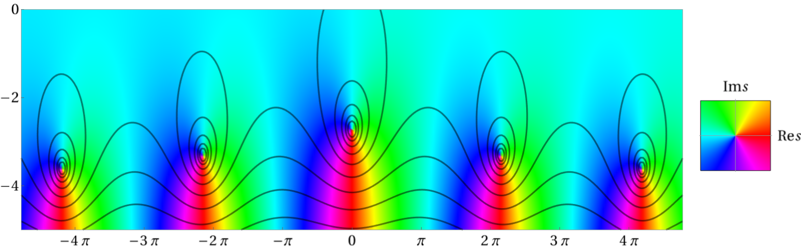
Figure D2: The complex plot of the derivative $f\left(s\right)=-i\partial m/\partial s-y$ of the integrand of Eq. 171 for $y=10$ computed for the model with $\lambda=0.12$ and $Z=51$. The color encodes the value of $\arg f$ according to the legend to the right, which stands for the complex plot of the function $f\left(s\right)=s$. One can observe that $f$ has 5 zeroes in the presented plot region. The imaginary parts of zeros are close to a corresponding multiple of $2\pi$. The black solid lines represent the contours of constant value of $\log_{10}\left|f\right|$ with the step of $0.2$, with the smallest value corresponding to $0.1$. The function grows exponentially in the lower half-plane, as evident from the fact that for $\text{Im}s\apprle 3.5$ the contours are approximately equidistant.

The integral over $s$ thus has a series of saddle points that can be described by the following equation:

$$S_{n}:=\frac{z_{n}}{i\kappa},\,\,\,\,\psi:=\frac{y-\left\langle y\right\rangle}{\lambda m_{1}\left(1\right)\sqrt{\frac{\pi}{2}}}\Rightarrow\frac{e^{z}}{\sqrt{z}}\left[1+O\left(\frac{1}{z}\right)\right]+O\left(\ln z\right)=\psi.$$ (213)

This equation possesses an infinite set of solutions $\left\{z_{n},n\in\mathbb{Z}\right\}$ that come in conjugate pairs, i. e. $z_{-n}=\overline{z_{n}}$, with each pair having an imaginary part of order $2\pi in$, as can be seen e.g. on D2. The asymptotic behavior of $z_{n}$ is captured by the following expression:

$$z_{n}\approx\begin{cases}-\frac{1}{2}W_{-1}\left(-\frac{2}{\psi^{2}}\right),&n=0,\\ -\frac{1}{2}W_{-\left(2n+1\right)}\left(-\frac{2}{\psi^{2}}\right),&n\in\mathbb{N},\\ -\frac{1}{2}W_{-2n}\left(-\frac{2}{\psi^{2}}\right),&-n\in\mathbb{N},\end{cases}$$ (214)

where $W_{k}\left(u\right)$ is the $k$-th branch of Lambert’s $W$-function. To obtain this approximation, we have neglected the error terms in Eq. 213. Each of the resulting saddle points produces a contribution to the value of the probability according to Eq. 192:

$$P^{\left(n\right)}\left(y\right)\sim\frac{1}{\sqrt{2\pi\kappa\left(y-\left\langle y\right\rangle\right)}}\cdot\exp\left\{-\frac{y-\left\langle y\right\rangle}{\kappa}\left[z_{n}-1+O\left(\frac{1}{z_{n}}\right)\right]+O\left(\ln z_{n}\right)\right\},$$ (215)

rendering the following result for the total probability:

$$P\left(y\right) \sim\frac{\exp\left\{-\frac{y-\left\langle y\right\rangle}{\kappa}\left[z_{0}-1+O\left(\frac{1}{z_{0}}\right)\right]+O\left(\ln z_{0}\right)\right\}}{\sqrt{2\pi\kappa\left(y-\left\langle y\right\rangle\right)}}$$

$$\times\left[1+\sum_{n\neq 0}\exp\left\{-\frac{y-\left\langle y\right\rangle}{\kappa}\left[z_{n}-z_{0}+O\left(\frac{1}{z_{n}}-\frac{1}{z_{0}}\right)\right]+O\left(\ln\frac{z_{n}}{z_{0}}\right)\right\}\right].$$ (216)

Because $z_{n}$ for $n\neq 0$ come in conjugate pairs, the whole expression is real as it should be. The range of applicability of this result is again controlled by the region of convergence of the Gaussian integral, i. e.

$$\left|\frac{d^{3}m_{2}}{dS^{3}}\cdot\left(\frac{d^{2}m_{2}}{dS^{2}}\right)^{-3/2}\right|\ll 1\Leftrightarrow\sqrt{\frac{\kappa}{y-\left\langle y\right\rangle}}\ll 1.$$ (217)

Due to the exponential behavior 212 of the $m_{2}$ function, each term of the resulting series is only available up to logarithmic accuracy and we cannot provide an estimation for the sum in Eq. 216. In addition, this analysis is unable to provide the exact value of $m\left(1\right)$, which is controlled by the form of the distribution $P\left(y\right)$ near its maximum. In order to complete both of these tasks, one has to use the exact expressions for $m_{2}$ (e. g. those available in the limit of weak coupling, see E). Nevertheless, this analysis provides us with insights into the asymptotic behavior of the probability $P\left(y\right)$ for large values of the argument.

According to Eq. 213, the real part of $z_{n}$ grows with $n$. While the exact rate of decay depends on the particular form of the errors terms that we have neglected, one expects that for sufficiently large value of $y$ only several first terms contribute to the sum in Eq. 216. In particular, one can establish the general form of the asymptotic tail of the distribution by using only the main saddle point:

$$\ln P\left(y\right)\sim\ln P^{\left(0\right)}\left(y\right)\sim-\frac{y-\left\langle y\right\rangle}{\kappa}\left[z_{0}-1+O\left(\frac{1}{z_{0}}\right)\right]+\ln\left[\frac{1}{\sqrt{2\pi\kappa\left(y-\left\langle y\right\rangle\right)}}\right]+O\left(\ln z_{0}\right),$$ (218)

where $z_{0}$ can be estimated according to Eq. 213 as

$$z_{0}\approx\ln\psi\cdot\left(1+O\left(\frac{1}{\ln\psi}\right)\right)+\frac{1}{2}\ln\ln\psi\cdot\left(1+O\left(\frac{1}{\ln\psi}\right)\right)+O\left(\frac{1}{\ln\psi}\right).$$ (219)

The precision of our calculations allows us to provide the final result in the following form:

$$\ln P\left(y\right)\sim-\frac{y-\left\langle y\right\rangle}{\kappa}\left[\ln\psi+\frac{1}{2}\ln\ln\psi-1\right]+\ln\frac{1}{\sqrt{2\pi\kappa\left(y-\left\langle y\right\rangle\right)}},\,\,\,\,\,\psi=\frac{y-\left\langle y\right\rangle}{\lambda m_{1}\left(1\right)\sqrt{\frac{\pi}{2}}}.$$ (220)

A practically important observation is that in a broad region of parameters this distribution is numerically close to a “squashed exponent” distribution of the form $\exp\left\{-Ay^{1+\beta}+\text{const}\right\}$ for some small parameter $\beta$, which is consistent with some experimental observations.

This result is also consistent with the Gaussian limit discussed in C.4, as the latter corresponds to $\kappa\ll 1$. Thus, according to the criteria 217, the asymptotic behavior 218 starts at

$$y-\left\langle y\right\rangle\gg\kappa=\sqrt{\left\langle\left\langle y^{2}\right\rangle\right\rangle/\lambda},$$ (221)

where the last equation is due to Eq. 191. Consequently, the probability at these values is already exponentially small, rendering the corresponding regime unobservable.

D.3 Probability function for $y>\left\langle y\right\rangle$: sub-leading corrections and secondary maxima

For moderately large values of $y$ and $\kappa$, the secondary saddle points bring in additional oscillatory behavior as seen on D1. The qualitative origin of these oscillations lies in the fact that each secondary saddle point has imaginary part of the order of $2\pi n,\,\,n\in\mathbb{Z}$. As a result of the latter, the contribution 215 of each saddle point exhibits damping oscillations w.r.t $y$ with period close to $\kappa/n$. One thus expects that all secondary contributions in the total sum 216 will demonstrate constructive interference as $y$ approaches

$$y_{n}=\left\langle y\right\rangle+\kappa n,\,\,\,\,\,n\in\mathbb{N}.$$ (222)

While the precision of our calculations does not allow us to demonstrate these oscillations explicitly, we can still use the leading asymptotic form to construct a meaningful model that illustrates such a behavior. By using the leading approximation 214 for $z_{n}$ and discarding the corrections despite their growing nature we can estimate the multiplicative correction to the probability as:

$$\ln\frac{P\left(y\right)}{P^{\left(0\right)}\left(y\right)}\sim\ln\left[1+2\text{Re}\sum_{n=1}^{\infty}\exp\left\{-\frac{y-\left\langle y\right\rangle}{\kappa}\left[-\frac{1}{2}W_{-\left(2n+1\right)}\left(-\frac{2}{\psi^{2}}\right)+\frac{1}{2}W_{-1}\left(-\frac{2}{\psi^{2}}\right)\right]\right\}\right],\,\,\,\,\,\psi=\frac{y-\left\langle y\right\rangle}{\lambda m_{1}\left(1\right)\sqrt{\frac{\pi}{2}}},$$ (223)

where we have taken into account that $z_{-n}=\overline{z}_{n}$ and thus the whole sum is real. It is worth specifying the asymptotic expression of the exponent at large $y$:

$$-\frac{1}{2}W_{-\left(2n+1\right)}\left(-\frac{2}{\psi^{2}}\right)+\frac{1}{2}W_{-1}\left(-\frac{2}{\psi^{2}}\right)=2\pi in\cdot\left[1+\frac{1}{2\ln\psi}+O\left(\frac{\ln\ln\psi}{\ln^{2}\psi}\right)\right]+\left[\left(\frac{\pi n}{\ln\psi}\right)^{2}+O\left(\frac{1}{\ln^{3}\psi}\right)\right].$$ (224)

We once again underscore that such an estimation cannot guarantee any sort of qualitative convergence and thus serves only illustrative purposes (at least because the correct estimation 215 contains the error term of the order $O\left(1/z_{n}\right)$ which is disregarded in the expression above). The plot of the resulting function for some values of the parameters is shown on the left plot of D3. Crucially, one can observe that the resulting expression exhibits oscillations with a slowly drifting period close to $\Delta y=\kappa$. The exact answer for the distribution function confirms this qualitative result, as evident from the neighboring right plot of D3 as well as from the data presented in the Main Text.

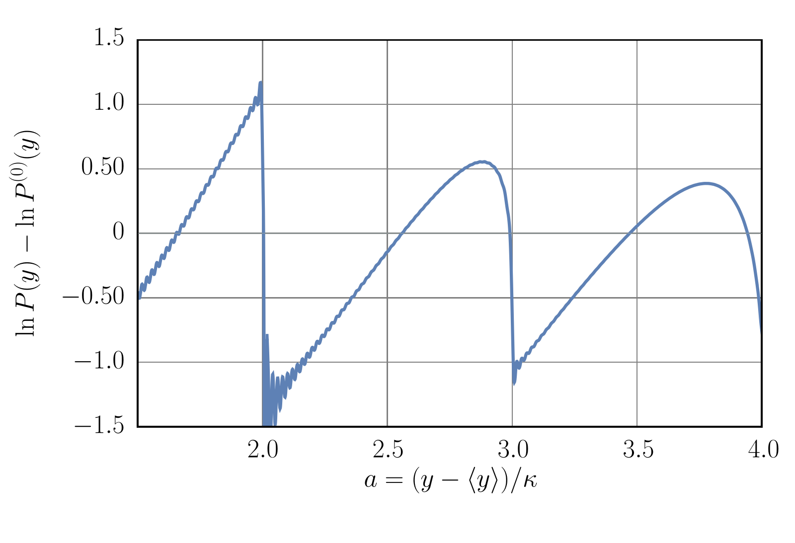
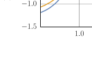
Figure D3: Plots of the logarithm of the multiplicative factor $f\left(y\right)$ distinguishing the leading asymptotic $P_{0}^{\left(0\right)}\left(y\right)$ behavior at large $y$ given by Eq. 220 and the true distribution of the dimensionless order parameter $P\left(y\right)=\exp\left\{f\left(y\right)\right\}\cdot P_{0}^{\left(0\right)}\left(y\right)$. The argument is given by $a=\left(y-\left\langle y\right\rangle\right)/\kappa$. The microscopical parameters of the model are $\lambda\approx 0.12$, $Z=51$ and $\kappa\approx 5.0$. Left. The multiplicative correction according to the qualitative estimation 223. The noise at moderate values of $a$ results from cutting the sum in Eq. 223 at a finite number of terms for the purposes of numerical evaluation. Right. The multiplicative correction according to various theoretical approximations for the true distribution. The blue curve represents the value of the integral 171 obtained by direct numerical integration. The orange line corresponds to saddle-point approximation of the integral 171 with all saddle point taken into account for $y>\left\langle y\right\rangle$. The green line reflects contribution of the leading purely imaginary saddle point only. When required, the exact $m$ function is used. The quantitative difference between the two plots is explained by the subleading corrections to the exponent of each term in Eq. 223 that are beyond the accuracy of the used expansions.

From the physics point of view, the secondary peaks are delivered by a certain spatial configurations of the disorder. Namely, the $n$-th secondary maximum of the distribution corresponds to the sites with exactly $n$ neighbors with small value of onsite disorder $\left|\xi_{k}\right|\apprle\Delta_{0}$. Indeed, suppose a given site $i$ has $n\sim 1$ such neighbors. Then the self-consistency equation 126 for this site $i$ reads:

$$\Delta_{i}=\sum_{j\in\partial i}f\left(\xi_{j},\Delta_{j}|\xi_{i}\right)\sim\sum_{j=1}^{n}\frac{\lambda}{\nu_{0}Z}+\sum_{j=n+1}^{Z}f\left(\xi_{j},\Delta_{j}|\xi_{i}\right)\sim\frac{n\lambda}{\nu_{0}Z}+\frac{n+1}{Z}\cdot\Delta_{0}$$

where we have used $\lambda/\nu_{0}Z$ as an approximation for the values of the right hand side for the chosen sites with small values of $\xi$, while the remaining sum was estimated by its mean field value. Rescaling this estimation to the units of $\Delta_{0}$ immediately leads us to Eq. 222.

The apparent sharpness of the peaks can be perceived as a consequence of Van Hove singularity in the distribution of the right hand side of the self-consistency equation. Indeed, at small values of $\xi$, the BSC root in Eq. 126 features a maximum, leading to a square root singularity in its distribution. The latter is subsequently contracted with the distribution of the order parameter itself, thus producing a shifted replica the main maximum of the distribution.

The presented explanation for the secondary peaks also admits a straightforward verification for each particular realization of the disorder. Given a solution to the self-consistency equation 126 in a particular realization of a random graph and disorder fields, one classifies all sites according to the exact number $k$ of neighbors with $\left|\xi\right|<\xi_{\min}$ where $\xi_{\min}$ is some threshold of order of several $\Delta_{0}$. By removing the $k$-th group from the complete set of $\Delta$ values, one expects to flatten out the corresponding secondary peak, while leaving all other peaks intact. The results of this procedure are presented on D4 and are rather confirmatory. The secondary peaks are not eliminated entirely by the described numerical classification because the distribution of the right hand side of the self-consistency equation exhibits a broad power-law tail away from the Van Hove singularity. As a result, there is no exact scale for the threshold parameter $\xi_{\min}$. This fact is also demonstrated on D4: depending on the exact value of the threshold, one can observe different degrees of deterioration of the secondary peaks.

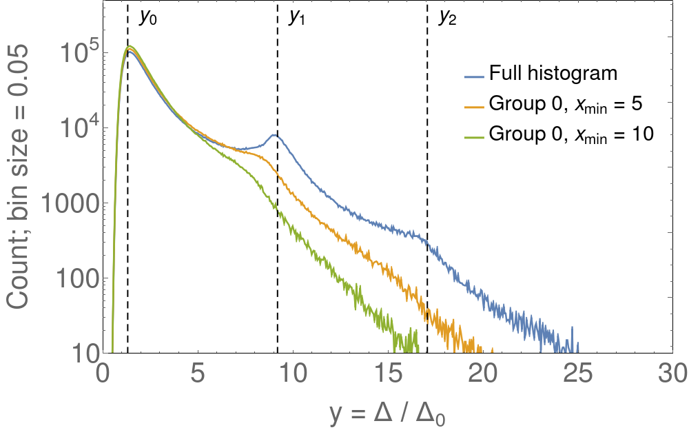
Figure D4: The plots of “filtered” histograms of the order parameter in a particular disorder realization with $N=2^{22}\approx 4.2\cdot 10^{6}$, $Z=51$, $\lambda=0.113$, corresponding to $Z_{\text{eff}}=1.43\cdot 10^{-2}$, $\kappa=7.88$. The curves are offset by a constant multiplier close to unity so that all curves are visible (otherwise they coincide with high precision). The vertical dashed lines denote the expected position of the maximum of the distribution according to Eq. 222, but with the value of $\left\langle y\right\rangle$ replaced with the actual position of main maximum $y_{\text{max}}\approx 1.3$. The noise present on both plots at large values of $y$ is due to statistical uncertainty, as can be deduced from the “count” value for these values of $y$. Left. Histograms obtained after excluding sets of sites with the corresponding number of neighbors satisfying $\left|\xi\right|<\xi_{\min}=5\Delta_{0}$. For instance, “Group 1” refers to the histogram obtained after excluding the sites with exactly one nearest neighbor that has $\left|\xi\right|<5\Delta_{0}$. One can see how the corresponding secondary peaks are suppressed in accordance to the fact that Group $n$ contributes to formation of the $n$-th peak. Right. Demonstration of the effect of various threshold values $\xi_{\min}=x_{\min}\cdot\Delta_{0}$ on the behavior of the histogram. One can observe how increasing the threshold suppresses all peaks except the main one.

The proposed explanation is also apparent from the theoretical analysis presented thus far. Indeed, the exponential behavior of the $m_{2}$ function originates from the vicinity of $w_{1}=1$ point in the integral 168. This region, in turn, corresponds to the values of the $f$ function achieved in the limit $\xi\ll\Delta$. As a result, each secondary peak effectively represents configurations with $n$ neighbors with small values of $\xi$, while the remaining neighbors form a background value of $\left\langle y\right\rangle$ in a mean field fashion.

A yet another consistency test is to examine the joint probability distribution $P\left(\xi_{j},\Delta_{i}\right)$ for some pair of neighboring sites $\left(i,j\right)$. Both numerical and analytical means then clear indicate that for small values of $\xi_{j}$ the conditional distribution experiences a well pronounced shift by the value of $f\left(\Delta,\xi\right)$, in full agreement with the proposed explanation. A representative example of numerical data is shown on D5.

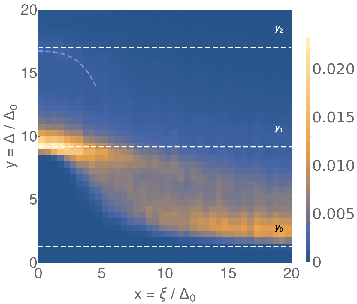
Figure D5: Density histogram of the joint probability distribution $P\left(\xi_{j},\Delta_{i}\right)$ for all pairs $\left(i,j\right)$ of neighboring sites in a particular disorder realization with $N=2^{22}\approx 4.2\cdot 10^{6}$, $Z=51$, $\lambda=0.113$, corresponding to $Z_{\text{eff}}=1.43\cdot 10^{-2}$, $\kappa=7.88$. The color represents the value of the probability density function according to the legend on the right. Horizontal dashed lines denote the expected position of the maximum of the marginal distribution $P\left(y\right)$ according to Eq. 222, but with the value of $\left\langle y\right\rangle$ replaced with the actual position of main maximum $y_{\text{max}}=1.3$. Note that the main maximum is situated at $y_{1}$ for small $x$ and approaches $y_{0}$ as $x$ grows. The light blue dashed line at the top left corner serves as a guide for the position of the secondary maximum wheres the latter can be resolved, although barely visible on the plot itself. The secondary maximum at small values of $x$ is thus situated close to $y_{2}$, in full agreement with the proposed interpretation.

We conclude this appendix by noting that the observed behavior of both the joint distribution $P\left(\xi_{i},\Delta_{j}\right)$ and the distribution of the order parameter $P\left(y\right)$ is expected to persist in the presence of the Onsager reaction term. As our analysis suggests, the positions of the maxima in both these distributions are determined solely by the direct influence of neighboring sites. On the other hand, the Onsager reaction term eliminates the “self-action” of the order parameter, i. e. its response to its own value via value of the order parameter on the neighboring sites. Therefore, such a term is incapable of altering the positions and strengths of the observed maxima of the distribution behavior qualitatively. For instance, one expects such an effect to be present if the self-consistency equations are solved on an indefinite directed Caley tree instead of a finite random regular graph, as visible e. g. on Figs 2 and 3 of Ref. [26].

Supplementary Material E Solution for the cumulant generating function $m$ in the limit of small $\lambda$

In this Appendix, we derive the analytical solution for the integral equations (167-168) in the limit of small BCS coupling constant $\lambda$. The resulting solution appears to be valid in the entire region of applicability of the self-consistency equation 87.

We seek the solution for both $m_{1}$ and $m_{2}$ in the form of a formal expansion in powers of small $\lambda$ up to the leading order. We start by discussing the magnitude of the functions in question. Let us consider the equation on $m_{1}$ first. As we will see later, the first two terms in Eq. 167 are both of order $O\left(\lambda^{0}\right)$. Assuming those to be the leading terms, one can see that the remaining contributions are all of order $O\left(\lambda^{1}\right)$ or smaller. Having these estimates hold, one can infer from Eq. 168 that the whole function $m_{2}$ is of order $O\left(\lambda^{1}\right)$ or smaller. As a result, we assert the following estimations for the functions in question:

$$m_{1}\left(w\right)=\kappa\cdot\left(w_{0}+w\right)+O\left(\lambda\right),\,\,\,\,\,w_{0}=O\left(\lambda^{0}\right),\,\,\,\,\,m_{2}\left(S|w\right)=O\left(\lambda^{1}\right)$$ (225)

where we have denoted

$$w_{0}:=m_{1}\left(0\right)/\kappa,$$ (226)

which is a suitable variable for further calculations.

This expansion can now be substituted in 168 to obtain $m_{2}$:

$$m_{2}\left(S|w\right)=\lambda\cdot\left[\left(w+w_{0}\right)\Phi_{0}\left(\kappa S\right)+\Phi_{1}\left(\kappa S\right)\right]+O\left(\lambda^{2}\right),$$ (227)

$$\Phi_{0}\left(\sigma\right) =\intop_{0}^{1}\frac{dw_{1}}{w_{1}^{2}\sqrt{1-w_{1}^{2}}}\left\{\exp\left\{i\sigma w_{1}\right\}-1-i\sigma w_{1}\right\}$$

$$=-\frac{1}{12}\sigma^{2}\left[3\pi\cdot\,_{1}F_{2}\left(\frac{1}{2};\frac{3}{2},2;-\frac{\sigma^{2}}{4}\right)+2i\sigma\cdot\,_{2}F_{3}\left(1,1;\frac{3}{2},2,\frac{5}{2};-\frac{\sigma^{2}}{4}\right)\right],$$ (228)

$$\Phi_{1}\left(\sigma\right)=\intop_{0}^{1}\frac{w_{1}dw_{1}}{\sqrt{1-w_{1}^{2}}}\left\{\exp\left\{i\sigma w_{1}\right\}-1-i\sigma w_{1}\right\}=i\frac{d^{3}\Phi_{0}\left(\sigma\right)}{d\sigma^{3}}-\frac{\pi}{4}i\sigma-1.$$ (229)

where $\,{}_{p}F_{q}$ is the generalized hypergeometric series:

$$\,{}_{p}F_{q}\left(a_{1},..a_{p};b_{1}...b_{q};z\right)=\sum_{k=0}^{\infty}\frac{\left(a_{1}\right)_{k}...\left(a_{p}\right)_{k}}{\left(b_{1}\right)_{k}...\left(b_{q}\right)_{k}}\frac{z^{k}}{k!},$$ (230)

with $\left(x\right)_{k}=\Gamma\left(x+k\right)/\Gamma\left(x\right)$ being the Pochhammer symbol.

With this expression at hand, one can turn back to the equation 167 for the $m_{1}$ function. It is convenient to use it in the form of expressions 175 and 177, rendering:

$$m_{1}\left(w\right)=\kappa\left(w+w_{0}\right)+\lambda\cdot\left\langle\left(y+\kappa w\right)\ln\frac{1}{y+\kappa w}-y\ln\frac{1}{y}\right\rangle+O\left(\lambda^{2}\right),$$ (231)

$$0=\frac{\pi}{4}\left(1+\lambda\ln\frac{1}{\kappa}\right)+\left\langle\frac{y}{\kappa}\right\rangle\ln\frac{1}{\kappa}+\left\langle\frac{y}{\kappa}\ln\frac{\kappa}{y}\right\rangle+\lambda\cdot\left\langle G\left(y/\kappa\right)\right\rangle.$$ (232)

where we have also retained $O\left(\lambda\right)$ contributions in the first equation in order to match with the precision of Eq. 227. The average values $\left\langle\bullet\right\rangle$ in this expressions are calculated as:

$$\left\langle\phi\left(y\right)\right\rangle=\intop_{0}^{\infty}dy\cdot\phi\left(y\right)P\left(y\right)\approx\intop_{\mathbb{R}-i0}\frac{d\sigma}{2\pi}\cdot\intop_{0}^{\infty}da\cdot\phi\left(\kappa a\right)\cdot\exp\left\{i\sigma w_{0}-i\sigma a+\lambda\cdot\left[w_{0}\Phi_{0}\left(\sigma\right)+\Phi_{1}\left(\sigma\right)\right]\right\}.$$

To obtain the last expression, we used the result 227 for the $m_{2}$ function and carried out substitutions $\sigma=\kappa s$, $a=y/\kappa$. It is thus convenient to rewrite the result as

$$m_{1}\left(w\right)=\kappa\left(w+w_{0}+\lambda\left[g_{1}\left(w_{0},w;\lambda\right)-g_{1}\left(w_{0},0;\lambda\right)\right]\right),$$ (233)

$$0=\frac{\pi}{4}\left(1+\lambda\ln\frac{1}{\kappa}\right)+w_{0}\ln\frac{1}{\kappa}+g_{1}\left(w_{0},0;\lambda\right)+\lambda\cdot g_{2}\left(w_{0};\lambda\right)+O\left(\lambda^{2}\right),$$ (234)

where we have used the exact identity $\left\langle y\right\rangle=m_{1}\left(0\right)=\kappa w_{0}$, and the $g$ functions are defined as

$$g_{1}\left(w_{0},w;\lambda\right)=\intop_{\mathbb{R}-i0}\frac{d\sigma}{2\pi}\cdot\intop_{0}^{\infty}da\cdot\left(a+w\right)\ln\frac{1}{a+w}\cdot\exp\left\{i\sigma w_{0}-i\sigma a+\lambda\cdot\left[w_{0}\Phi_{0}\left(\sigma\right)+\Phi_{1}\left(\sigma\right)\right]\right\},$$ (235)

$$g_{2}\left(w_{0};\lambda\right)=\intop_{0}^{1}dw\cdot\sqrt{1-w_{1}^{2}}\cdot\frac{g_{1}\left(w_{0},w_{1};\lambda\right)-g_{1}\left(w_{0},0;\lambda\right)}{w_{1}}.$$ (236)

To obtain the expression for $g_{2}$, we have used the integral representation 178 for the $G$ function. We now need to develop a proper approximation for $g_{1}$ function. Because we expect $w_{0}$ to be large, as it follows from the previous subsection, it is valid to seek a formal expansion of $g_{1}$ in powers of $1/w_{0}$. It is convenient to use the following integral representation for the $a$-dependence of the integrand in Eq. 235:

$$x\ln\frac{1}{x}=-x-\intop_{0}^{\infty}dt\cdot\frac{e^{-xt}+e^{-t}xt-1}{t^{2}}.$$ (237)

With the use of this representation, we can rewrite the expression $g_{1}$ as:

$$g_{1}\left(w_{0},w;\lambda\right)=-\left(w_{0}+w\right)-\intop_{0}^{\infty}dt\left[\frac{\exp\left\{-t\left(w_{0}+w\right)+\lambda\cdot\left[w_{0}\Phi_{0}\left(it\right)+\Phi_{1}\left(it\right)\right]\right\}+e^{-t}\left(w_{0}+w\right)t-1}{t^{2}}\right].$$ (238)

To obtain this result, the integral over $a$ was taken exactly, and the subsequent integration over $\sigma$ was carried out by means of Cauchy theorem. Before we move on, it should be noted, that the integral over $t$ should be formally cut at $t_{0}\sim\exp\left\{1/\lambda\right\}$. Indeed, according to asymptotic expression 196 derived earlier, the $\Phi_{0}$ term brings in a contribution whose real part grows as $+\lambda w_{0}\cdot t\ln t$ at large $t$, so that it eventually dominates the linear decay provided by the first term in the exponent. However, this happens only at $t\sim t_{0}$, where the expression for $m_{2}$ itself ceases to work, as discussed in C. The integral itself gains its value at $t\sim\left(w_{0}+w\right)^{-1}$ due to the first term, thus allowing one to treat the expression as convergent.

The expression 238 is thus suitable for expanding in powers of $\lambda$, rendering:

$$g_{1}\left(w_{0},w;\lambda\right) =-\left(w_{0}+w\right)-\intop_{0}^{\infty}dt\left[\frac{e^{-t\left(w_{0}+w\right)}+e^{-t}\left(w_{0}+w\right)t-1}{t^{2}}\right]$$

$$-\lambda\intop_{0}^{\infty}dt\cdot e^{-t\left(w_{0}+w\right)}\cdot\frac{w_{0}\Phi_{0}\left(it\right)+\Phi_{1}\left(it\right)}{t^{2}}+O\left(\lambda^{2}\right).$$ (239)

Finally, integrals over $t$ can be evaluated, resulting in:

$$g_{1}\left(w_{0},w;\lambda\right)=\left(w_{0}+w\right)\ln\frac{1}{w_{0}+w}-\lambda\cdot H\left(w_{0},w\right)+O\left(\lambda^{2}\right),$$ (240)

$$H\left(w_{0},w\right)=\intop_{0}^{1}\frac{dw_{1}}{\sqrt{1-w_{1}^{2}}}\cdot\left(w_{0}+w_{1}^{3}\right)\cdot\frac{\left(w+w_{0}+w_{1}\right)\ln\left(\frac{w_{1}+w+w_{0}}{w+w_{0}}\right)-w_{1}}{w_{1}^{2}}.$$ (241)

Now, the result can be used to calculate the $g_{2}$ term. Within the required precision, we only need to use the leading term in Eq. 240, rendering:

$$g_{2}\left(w_{0};\lambda\right)=\intop_{0}^{1}dw\cdot\sqrt{1-w_{1}^{2}}\cdot\frac{\left(w_{0}+w_{1}\right)\ln\frac{1}{w_{0}+w_{1}}-w_{0}\ln\frac{1}{w_{0}}}{w_{1}}\equiv G\left(w_{0}\right)+O\left(\lambda\right),$$ (242)

where $G$ is the function defined in Eq. 178.

At this point, it is worth noting that the derived expression 240 for $g_{1}$ possesses a transparent qualitatively interpretation. According to 235, the $g_{1}$ function represents the mean value of the form

$$g_{1}\left(w_{0},w;\lambda\right)=\left\langle\frac{y+\kappa w}{\kappa}\ln\frac{\kappa}{y+\kappa w}\right\rangle,$$ (243)

where the average is taken over the exact distribution $P\left(y\right)$ function of the order parameter. On the other hand the value of $w_{0}$ also corresponds to the average value of the form $\left\langle y/\kappa\right\rangle$. One can thus see that the leading term in the approximation 240 for the $g_{1}$ function corresponds to replacing the full distribution $P\left(y\right)$ with a $\delta$-function centered at the mean value, i. e. $\delta\left(y-\kappa w_{0}\right)$. The sub-leading corrections to $g_{1}$ are then obtained by treating the actual form of the distribution as a perturbation on top of the trial distribution. This appears to be sufficient to determine the value of $w_{0}$ with the required accuracy solely because the averaged functions $y$ and $y\ln 1/y$ differ by a slow function that does not contribute substantially to the result unless the underlying distribution possesses fat tails. That is why, it would be qualitatively wrong to perform such an approximation for other averages. Consider, for instance, low order cumulants: they vanish identically for a $\delta$-like distribution, but from the form of the cumulant generating function given by $m$ itself one can tell that in our problem they are all of the same order.

Collecting everything together, one obtains the following set of equations for the $m_{1}$ function:

$$m_{1}\left(w\right)=\kappa\left(w+w_{0}\right)+\lambda\cdot\left[\left(w_{0}+w\right)\ln\frac{1}{w_{0}+w}-w_{0}\ln\frac{1}{w_{0}}\right]+O\left(\lambda^{2}\right),$$ (244)

$$0=\frac{\pi}{4}\left(1+\lambda\ln\frac{1}{\kappa}\right)+w_{0}\ln\frac{1}{\kappa}+w_{0}\ln\frac{1}{w_{0}}+\lambda\cdot F\left(w_{0}\right)+O\left(\lambda^{2}\right),$$ (245)

$$F\left(w_{0}\right) =G\left(w_{0}\right)-H\left(w_{0},0\right)=\intop_{0}^{1}dw_{1}\cdot\left[\frac{w_{1}^{2}+\left(1-w_{1}^{2}\right)\ln\frac{1}{w_{0}}}{\sqrt{1-w_{1}^{2}}}+\frac{\left(w_{0}+w_{1}\right)^{2}\ln\frac{w_{0}}{w_{0}+w_{1}}+w_{0}w_{1}}{w_{1}^{2}\sqrt{1-w_{1}^{2}}}\right]$$

$$=\frac{\pi}{4}\left(1+\ln\frac{1}{w_{0}}\right)+\frac{\pi}{4}\left(2w_{0}^{2}+3+2\ln 2-\left(\frac{4}{\pi}+\pi\right)w_{0}-2\ln\frac{1}{w_{0}}\right)$$

$$+w_{0}\left[\text{arccos}\frac{1}{w_{0}}\right]^{2}-w_{0}\left[w_{0}\sqrt{w_{0}^{2}-1}-\ln\left(w_{0}-\sqrt{w_{0}^{2}-1}\right)\right]\text{arccos}\frac{1}{w_{0}}$$

$$+\left[i\cdot\text{Li}_{2}\left(\frac{i-\sqrt{w_{0}^{2}-1}}{w_{0}}\right)-i\cdot\text{Li}_{2}\left(\frac{-i+\sqrt{w_{0}^{2}-1}}{w_{0}}\right)-\frac{i\pi}{4}\ln\left(\frac{-w_{0}^{2}+2\sqrt{1-w_{0}^{2}}+2}{w_{0}^{2}}\right)\right],$$ (246)

where $\text{Li}_{n}\left(z\right)$ is the polylogarithm function 179. Similarly to expression 178 for the $G$ function, the $F$ function is purely real for all $w_{0}>0$ and represents a holomorphic function of $w_{0}\in\mathbb{C}$ with a branch cut along $\left[-\infty,w_{0}\right]$.

From this result, we can also infer the actual limit of applicability of the proposed procedure. Indeed, at large $w_{0}$ the sub-leading term behaves as

$$F\left(w_{0}\gg 1\right)=\frac{\pi}{4}\left(1+\ln\frac{1}{w_{0}}\right)-\frac{1}{3w_{0}}+O\left(\frac{1}{w_{0}^{2}}\right),$$ (247)

so that the obtained series for $g_{1}+\lambda g_{2}$ is governed by the parameter $\lambda/w_{0}\ll 1$. Quite conveniently, this also happens to coincide with the criteria of applicability of the expression 227 for the $m_{2}$ function.

As a by-product of the presented calculation, one can infer the explicit result of the typical value of the distribution. The latter is defined as

$$y_{\text{typ}}:=\exp\left\{\left\langle\ln y\right\rangle\right\}.$$ (248)

One can observe that it is connected to the derivative of $g_{1}$ function as:

$$\frac{\partial g_{1}}{\partial w}\left(w_{0},0;\lambda\right)\equiv\left[\frac{\partial}{\partial w}\left\langle\frac{y+\kappa w}{\kappa}\ln\frac{\kappa}{y+\kappa w}\right\rangle\right]_{w=0}=\left\langle\ln\frac{\kappa}{y}\right\rangle-1\equiv\ln\kappa-\ln y_{\text{typ}}-1.$$ (249)

Consequently, the typical value reads:

$$y_{\text{typ}}=\kappa\cdot\exp\left\{-\left[\frac{\partial g_{1}}{\partial w}\left(w_{0},0;\lambda\right)+1\right]\right\}=\kappa w_{0}\cdot\exp\left\{-\lambda\cdot\frac{\partial H}{\partial w}\left(w_{0},0\right)+O\left(\lambda^{2}\right)\right\}=\kappa w_{0}\cdot\exp\left\{-\frac{\pi\lambda}{4w_{0}}+O\left(\lambda^{2}\right)\right\}.$$ (250)

To obtain the last expression, we have evaluated the required expression for the $H$ function.

Solving the resulting equation 245 for $w_{0}$ up to the available precision renders

$$w_{0}=w_{0}^{\left(0\right)}+\lambda\cdot w_{0}^{\left(1\right)}+O\left(\lambda^{2}\right),\,\,\,\,\,w_{0}^{\left(0\right)}=\frac{\pi/4}{W\left(\pi\kappa/4\right)},\,\,\,\,\,w_{0}^{\left(1\right)}=\frac{\frac{\pi}{4}\ln\frac{1}{\kappa}+F\left(w_{0}^{\left(0\right)}\right)}{\ln\kappa w_{0}^{\left(0\right)}+1}.$$ (251)

The result suggests that the presented derivation is applicable when

$$w_{0}^{\left(0\right)}\apprge\lambda\Leftrightarrow\kappa\apprle\frac{4}{\pi}\exp\left\{\frac{\pi}{4}\frac{1}{\lambda}\right\}.$$ (252)

This corresponds to the following limitation on the value of $Z$:

$$Z\apprge Z^{*}=\frac{\lambda}{2\nu_{0}\Delta_{0}\cdot\frac{4}{\pi}\exp\left\{\frac{\pi}{4}\frac{1}{\lambda}\right\}}\sim\frac{\pi}{4}\cdot\frac{\lambda}{4\nu_{0}\varepsilon_{D}}\cdot\exp\left\{\frac{1}{\lambda}\left(1-\frac{\pi}{4}\right)\right\}.$$ (253)

Remarkably, this scale is exponentially smaller than $Z_{1}=\lambda\cdot\exp\left\{1/2\lambda\right\}$, with the latter being the scale suggested by [23] as the lower limit below which the original self-consistency equation is rendered inapplicable, see the discussion after Eq. (LABEL:saddle-point_order-parameter) for details. Consequently, the developed approximation covers the entire region of applicability of the proposed model for sufficiently small $\lambda$.

Let us now summarize the obtained results: we have derived the following analytical solution to the integral equations (167-168):

$$m_{1}\left(w\right)=\kappa\left(w+w_{0}\right)+\lambda\cdot\left[\left(w_{0}+w\right)\ln\frac{1}{w_{0}+w}-w_{0}\ln\frac{1}{w_{0}}\right],$$ (254)

$$m_{2}\left(S|w\right)=\lambda\cdot\left[\left(w+w_{0}\right)\Phi_{0}\left(\kappa S\right)+\Phi_{1}\left(\kappa S\right)\right],$$ (255)

$$w_{0}=w_{0}^{\left(0\right)}+\lambda\cdot w_{0}^{\left(1\right)},\,\,\,\,\,w_{0}^{\left(0\right)}=\frac{\pi/4}{W\left(\pi\kappa/4\right)},\,\,\,\,w_{0}^{\left(1\right)}=\frac{\frac{\pi}{4}\ln\frac{1}{\kappa}+F\left(w_{0}^{\left(0\right)}\right)}{\ln\kappa w_{0}^{\left(0\right)}+1},$$ (256)

where $\Phi_{i}$ are special functions given by Eq.-s (228-229), and $F$ is given by Eq. 246. The solution is controlled by the parameter $\lambda/w_{0}\ll 1$, which turns out to be small in the entire limit of applicability of the proposed model. The presented solution comprises all previously discussed special cases. For instance, one can formally expand these equations in the limit $\kappa\ll 1$, corresponding to the Gaussian regime. The result then reduces back to expressions (183-184), thus successfully reproducing the large $Z_{\text{eff}}$ limit. In the opposite limit of $\kappa\apprge 1$, the expressions (254-256) provide a quantitative demonstration for the asymptotic behavior described in D.

Supplementary Material F The effect of smooth energy dependence of the matrix element

In the simplified model discussed in C, we have ignored the dependence of the matrix element $D\left(\xi\right)$ on the energy difference, replacing it with a constant value given by $D\left(0\right)$. In this section, we restore this dependence and discuss its effect on our results.

F.1 Qualitative discussion

Let us first briefly discuss the role of the $D$ function within the mean-field approach described in A. In the simplified version of the theory we have been discussing thus far, the logarithmically divergent integral in Eq. 88 was cut off at energies of order $E_{F}$ originating purely from the behavior of the density of states $\nu\left(\xi\right)$. The main role of the energy dependence $D\left(\xi\right)$ is to provide a more physical upper limit cut-off of the order of $\varepsilon_{D}$, as it was shown in A. However, the difference between the effect of $\nu\left(\xi\right)$ and $D\left(\xi\right)$ is that the latter endows the order parameter with and additional dependence on the onsite value of the disorder field $\xi_{0}$. In other words, one now has to describe not just the value of $\Delta_{0}$, but the whole function $\Delta\left(\xi_{0}\right)$. As it is demonstrated in A, the profile of $\Delta\left(\xi_{0}\right)$ resembles that of $D\left(\xi_{0}\right)$ itself, and thus the emergent typical scale of $\xi_{0}$-dependence in also given by $\xi_{0}\sim\varepsilon_{D}$.

Connected to the mean-field equation is the question of the actual number of sites participating in the superconducting order. Indeed, in the current version of the model, each site develops its own value of the order parameter of order $\Delta_{0}$, regardless of the onsite value of $\xi$. On the other hand, already at the level of the mean-field equation it is clear that only sites with energies $\left|\xi\right|\apprle\varepsilon_{D}$ can participate in the formation of superconducting state due to the limitation on maximum energy transfer. In other words, we expect the actual joint probability distribution of $\xi$ and $\Delta$ on a given site to behave as

$$P\left(\xi,\Delta\right)\sim\begin{cases}\frac{\varepsilon_{D}}{E_{F}}\cdot P_{0}\left(\xi,\Delta\right),&\left|\xi\right|\apprle\varepsilon_{D},\\ \left(1-\frac{\varepsilon_{D}}{E_{F}}\right)\cdot\nu\left(\xi\right)\cdot\delta\left(\Delta\right),&\left|\xi\right|\apprge\varepsilon_{D},\end{cases}$$ (257)

where $P_{0}$ is the low-energy joint distribution 171 found in the previous section. The leading prefactors in both expressions ensure normalization and reflect the fact that only $\sim N\cdot\varepsilon_{D}/E_{F}$ of all $N$ sites in the system actually develop superconducting ordering. Therefore, the role of the $\eta$ function in a more accurate version of the theory is to exclude the sites deep within the Fermi sea from superconducting correlations.

F.2 Equations for the $m$ function

Let us now turn to quantitative description of the outlined differences. From the considerations above one concludes that the $m$ function and all associated objects should also exhibit a slow dependence on the onsite value of $x=\xi/\Delta_{0}$. The corresponding counterpart of the equation 137 for the $r$ function now reads:

$$r\left(S|x,y\right) =\intop_{\mathbb{R}}dx_{1}\intop_{0}^{\infty}dy_{1}\cdot\left[\exp\left\{iS\frac{f\left(\Delta_{0}x_{1},\Delta_{0}y_{1}|\Delta_{0}x\right)}{\Delta_{0}}\right\}-1\right]\cdot\frac{\nu\left(\Delta_{0}x_{1}\right)}{2\nu_{0}}$$

$$\times\intop_{\mathbb{R}-i0}\frac{ds}{2\pi}\cdot\exp\left\{is\frac{f\left(\Delta_{0}x,\Delta_{0}y|\Delta_{0}x_{1}\right)}{\Delta_{0}}\right\}\frac{\partial}{\partial y_{1}}\left\{\left[\intop_{\infty}^{y_{1}}dy_{1}^{{}^{\prime}}\exp\left\{-isy_{1}^{{}^{\prime}}\right\}\right]\cdot\exp\left\{Z_{\text{eff}}\cdot r\left(s|x_{1},y_{1}\right)\right\}\right\}.$$ (258)

It is convenient to parametrize the $f$ function as

$$f\left(\xi,\Delta|\xi_{0}\right)=\Delta_{0}\cdot\kappa\cdot\omega\left(\xi/\Delta\right)\cdot\eta\left(\frac{\xi-\xi_{0}}{\Delta_{0}}\right),$$ (259)

where $\eta$ is the function determining the energy dependence of the matrix element (c.f. with 90):

$$\eta\left(x\right)\equiv u\left(\Delta_{0}x\right)=D\left(\Delta_{0}x\right)/D\left(0\right).$$ (260)

One can also introduce the following parametrization for the $r$ function:

$$r\left(S|x,y\right):=r\left(S|w=\omega\left(x/y\right),x\right),$$ (261)

so that the $x$-dependence is explicitly factorized into the low-energy part corresponding to $w$ argument and high-energy dependence originating from the presence of the $\eta$ function. Extracting the main logarithmic divergence according to the procedure outlined in C.3 produces the following set of equations:

$$r\left(S|w,\underline{x}\right)=\left[\text{target eq.}-\Delta r\right]+\left[\Delta r-\Delta r_{f}\right]+\Delta r_{f},$$ (262)

$$\left[\text{target eq.}-\Delta r\right] =\intop_{\mathbb{R}}dx_{1}\intop_{0}^{\infty}dy_{1}\cdot\left[\exp\left\{iS\kappa\cdot\omega\left(x_{1}/y_{1}\right)\cdot\underline{\eta\left(x-x_{1}\right)}\right\}-1-iS\kappa\cdot\omega\left(x_{1}/y_{1}\right)\cdot\underline{\eta\left(x-x_{1}\right)}\right]\cdot\frac{\nu\left(\Delta_{0}x_{1}\right)}{2\nu_{0}}$$

$$\times\intop_{\mathbb{R}-i0}\frac{ds}{2\pi}\cdot\exp\left\{is\kappa\cdot w\cdot\underline{\eta\left(x_{1}-x\right)}\right\}\frac{\partial}{\partial y_{1}}\left\{\left[\intop_{\infty}^{y_{1}}dy_{1}^{{}^{\prime}}e^{-isy_{1}^{{}^{\prime}}}\right]\cdot\exp\left\{Z_{\text{eff}}\cdot r\left(s|\omega\left(x_{1}/y_{1}\right),\underline{x_{1}}\right)\right\}\right\},$$ (263)

$$\left[\Delta r-\Delta r_{r}\right] =\intop_{\mathbb{R}}dx_{1}\intop_{0}^{\infty}dy_{1}\cdot iS\kappa\cdot\omega\left(x_{1}/y_{1}\right)\cdot\underline{\eta\left(x-x_{1}\right)}\cdot\frac{\nu\left(\Delta_{0}x_{1}\right)}{2\nu_{0}}\cdot\intop_{\mathbb{R}-i0}\frac{ds}{2\pi}\cdot\exp\left\{is\kappa\cdot w\cdot\underline{\eta\left(x_{1}-x\right)}\right\}$$

$$\times\frac{\partial}{\partial y_{1}}\left\{\left[\intop_{\infty}^{y_{1}}dy_{1}^{{}^{\prime}}e^{-isy_{1}^{{}^{\prime}}}\right]\left(\exp\left\{Z_{\text{eff}}\cdot r\left(s|\omega\left(x_{1}/y_{1}\right),\underline{x_{1}}\right)\right\}-\exp\left\{Z_{\text{eff}}\cdot r\left(s|0,\underline{x_{1}}\right)\right\}\right)\right\},$$ (264)

$$\left[\Delta r_{r}-\Delta r_{rf}\right] =\intop_{\mathbb{R}}dx_{1}\intop_{0}^{\infty}dy_{1}\cdot iS\kappa\cdot\left[\omega\left(x_{1}/y_{1}\right)-y_{1}\omega\left(x_{1}\right)\right]\cdot\underline{\eta\left(x-x_{1}\right)}\cdot\frac{\nu\left(\Delta_{0}x_{1}\right)}{2\nu_{0}}$$

$$\times\intop_{\mathbb{R}-i0}\frac{ds}{2\pi}\cdot\exp\left\{is\kappa\cdot w\cdot\underline{\eta\left(x_{1}-x\right)}\right\}\cdot\frac{\partial}{\partial y_{1}}\left\{\left[\intop_{\infty}^{y_{1}}dy_{1}^{{}^{\prime}}e^{-isy_{1}^{{}^{\prime}}}\right]\cdot\exp\left\{Z_{\text{eff}}\cdot r\left(s|0,\underline{x_{1}}\right)\right\}\right\},$$ (265)

$$\Delta r_{rf} =\intop_{\mathbb{R}}dx_{1}\intop_{0}^{\infty}dy_{1}\cdot iS\kappa\cdot y_{1}\omega\left(x_{1}\right)\cdot\underline{\eta\left(x-x_{1}\right)}\cdot\frac{\nu\left(\Delta_{0}x_{1}\right)}{2\nu_{0}}$$

$$\times\intop_{\mathbb{R}-i0}\frac{ds}{2\pi}\cdot\exp\left\{is\kappa\cdot w\cdot\underline{\eta\left(x_{1}-x\right)}\right\}\cdot\frac{\partial}{\partial y_{1}}\left\{\left[\intop_{\infty}^{y_{1}}dy_{1}^{{}^{\prime}}e^{-isy_{1}^{{}^{\prime}}}\right]\cdot\exp\left\{Z_{\text{eff}}\cdot r\left(s|0,\underline{x_{1}}\right)\right\}\right\},$$ (266)

where underlined are the differences of these expressions to their counterparts in C.2. Similarly to the calculations of C.2, the next step is to treat the functions $\eta\left(x\right)$, $\nu\left(x\right)$ and $r\left(...,x\right)$ as constant in all expressions where the corresponding integral is convergent at the scale $x\sim 1$. This allows one to rewrite the equations above as

$$\left[\text{target eq.}-\Delta r\right] =\frac{1}{2}\intop_{\mathbb{R}}dx_{1}\intop_{0}^{\infty}dy_{1}\cdot\left[\exp\left\{iS\kappa\cdot\omega\left(x_{1}/y_{1}\right)\cdot\underline{\eta\left(x\right)}\right\}-1-iS\kappa\cdot\omega\left(x_{1}/y_{1}\right)\cdot\underline{\eta\left(x\right)}\right]$$

$$\times\intop_{\mathbb{R}-i0}\frac{ds}{2\pi}\cdot\exp\left\{is\kappa\cdot w\cdot\underline{\eta\left(x\right)}\right\}\frac{\partial}{\partial y_{1}}\left\{\left[\intop_{\infty}^{y_{1}}dy_{1}^{{}^{\prime}}e^{-isy_{1}^{{}^{\prime}}}\right]\cdot\exp\left\{Z_{\text{eff}}\cdot r\left(s|\omega\left(x_{1}/y_{1}\right),\underline{0}\right)\right\}\right\},$$ (267)

$$\left[\Delta r-\Delta r_{r}\right] =iS\kappa\underline{\eta\left(x\right)}\cdot\frac{1}{2}\intop_{\mathbb{R}}dx_{1}\intop_{0}^{\infty}dy_{1}\cdot\omega\left(x_{1}/y_{1}\right)\cdot\intop_{\mathbb{R}-i0}\frac{ds}{2\pi}\cdot\exp\left\{is\kappa\cdot w\cdot\underline{\eta\left(x\right)}\right\}$$

$$\times\frac{\partial}{\partial y_{1}}\left\{\left[\intop_{\infty}^{y_{1}}dy_{1}^{{}^{\prime}}e^{-isy_{1}^{{}^{\prime}}}\right]\left(\exp\left\{Z_{\text{eff}}\cdot r\left(s|\omega\left(x_{1}/y_{1}\right),\underline{0}\right)\right\}-\exp\left\{Z_{\text{eff}}\cdot r\left(s|0,\underline{0}\right)\right\}\right)\right\},$$ (268)

$$\left[\Delta r_{r}-\Delta r_{rf}\right] =iS\kappa\underline{\eta\left(x\right)}\cdot\frac{1}{2}\intop_{\mathbb{R}}dx_{1}\intop_{0}^{\infty}dy_{1}\cdot\left[\omega\left(x_{1}/y_{1}\right)-y_{1}\omega\left(x_{1}\right)\right]$$

$$\times\intop_{\mathbb{R}-i0}\frac{ds}{2\pi}\cdot\exp\left\{is\kappa\cdot w\cdot\underline{\eta\left(x\right)}\right\}\cdot\frac{\partial}{\partial y_{1}}\left\{\left[\intop_{\infty}^{y_{1}}dy_{1}^{{}^{\prime}}e^{-isy_{1}^{{}^{\prime}}}\right]\cdot\exp\left\{Z_{\text{eff}}\cdot r\left(s|0,\underline{0}\right)\right\}\right\},$$ (269)

$$\Delta r_{rf} =\intop_{\mathbb{R}}dx_{1}\intop_{0}^{\infty}dy_{1}\cdot iS\kappa\cdot y_{1}\omega\left(x_{1}\right)\cdot\underline{\eta\left(x-x_{1}\right)}\cdot\frac{\nu\left(\Delta_{0}x_{1}\right)}{2\nu_{0}}$$

$$\times\intop_{\mathbb{R}-i0}\frac{ds}{2\pi}\cdot\exp\left\{is\kappa\cdot w\cdot\underline{\eta\left(x_{1}-x\right)}\right\}\cdot\frac{\partial}{\partial y_{1}}\left\{\left[\intop_{\infty}^{y_{1}}dy_{1}^{{}^{\prime}}e^{-isy_{1}^{{}^{\prime}}}\right]\cdot\exp\left\{Z_{\text{eff}}\cdot r\left(s|0,\underline{x_{1}}\right)\right\}\right\}.$$ (270)

Note that the last expression remained intact, as it still contains a logarithmic integral over $x_{1}$. One then proceeds to simplifying these expressions in a way similar to that presented in C.2. The result then reads:

$$m\left(S|w,\underline{x}\right):=Z_{\text{eff}}\cdot r\left(S|w,\underline{x}\right)=iSm_{1}\left(w,\underline{x}\right)+m_{1}\left(S|w,\underline{x}\right),$$ (271)

$$m_{2}\left(S|w,x\right)=\lambda\intop_{0}^{1}dw_{1}\cdot\frac{\exp\left\{iS\kappa\underline{\eta\left(x\right)}\cdot w_{1}\right\}-1-iS\kappa\underline{\eta\left(x\right)}\cdot w_{1}}{w_{1}^{2}\sqrt{1-w_{1}^{2}}}\cdot\left[1-w_{1}\left(1-w_{1}^{2}\right)\frac{\partial}{\partial w_{1}}\right]\cdot\left[\frac{\kappa w\underline{\eta\left(x\right)}+m_{1}\left(w_{1},\underline{0}\right)}{\kappa}\right],$$ (272)

$$m_{1}\left(w,\underline{x}\right) =\underline{\eta\left(x\right)}\cdot\lambda\intop_{0}^{1}dw_{1}\cdot\sqrt{1-w_{1}^{2}}\cdot\frac{m_{1}\left(w_{1},\underline{0}\right)-m_{1}\left(0,\underline{0}\right)}{w_{1}}$$

$$+\underline{\eta\left(x\right)}\cdot\lambda\intop_{0}^{\infty}dy_{1}\cdot y_{1}\ln\frac{1}{y_{1}}\cdot\intop_{\mathbb{R}-i0}\frac{ds}{2\pi}\cdot\exp\left\{is\kappa\underline{\eta\left(x\right)}\cdot w\right\}\cdot\exp\left\{m\left(s|0,\underline{0}\right)-isy_{1}\right\}$$

$$+\lambda\intop_{\mathbb{R}}dx_{1}\cdot\omega\left(x_{1}\right)\cdot\underline{\eta\left(x-x_{1}\right)}\cdot\frac{\nu\left(\Delta_{0}x_{1}\right)}{2\nu_{0}}\cdot\left\{\kappa w\cdot\underline{\eta\left(x_{1}-x\right)}+m_{1}\left(0,\underline{x_{1}}\right)\right\}.$$ (273)

In order to further simply the last term in the equation on $m_{1}$, one considers the following identity:

$$m_{1}\left(0,x\right)-\eta\left(x\right)m_{1}\left(0,0\right)=\lambda\intop_{\mathbb{R}}dx_{1}\cdot\omega\left(x_{1}\right)\cdot\frac{\nu\left(\Delta_{0}x_{1}\right)}{2\nu_{0}}\cdot m_{1}\left(0,x_{1}\right)\cdot\left(\eta\left(x-x_{1}\right)-\eta\left(x\right)\eta\left(x_{1}\right)\right),$$ (274)

which is obtained by using Eq. 273 for both instance of $m$ in the right hand side. As it follows from the qualitative considerations in the beginning of this Appendix, we expect $m_{1}\left(0,x_{1}\right)$ to depend on $x_{1}$ only at the scale $x_{1}\sim\varepsilon_{D}/\Delta_{0}$. The resulting integral over $x_{1}$ is thus governed by $x_{1}\sim\varepsilon_{D}/\Delta_{0}$, so that one can replace $\omega\left(x_{1}\right)$ with $1/\left|x_{1}\right|$, similarly to the derivation of Eq. 273. We then observe that the value of $m_{1}\left(0,x\right)$ is given by the mean-field answer corresponding to Eq. 92:

$$m_{1}\left(0,x\right)=m_{1}\left(0,0\right)\cdot d\left(\Delta_{0}\cdot x\right),$$ (275)

where $d\left(\xi\right)$ is the function obeying Eq. 94. Because the $d$ function also happens to describe the exact energy dependence of the mean-field order parameter $\Delta_{0}\left(\xi\right)$, one can evaluated explicitly the value of the integral containing $m_{1}$ in Eq. 273 due to the self-consistency equation 93:

$$\lambda\intop_{\mathbb{R}}dx_{1}\cdot\omega\left(x_{1}\right)\cdot\eta\left(x-x_{1}\right)\cdot\frac{\nu\left(\Delta_{0}x_{1}\right)}{2\nu_{0}}m_{1}\left(0,x_{1}\right)=m_{1}\left(0,0\right)\cdot d\left(\Delta_{0}x\right)$$ (276)

The equation on $m_{1}$ can then be rewritten as

$$m_{1}\left(w,\underline{x}\right) =\underline{\eta\left(x\right)}\cdot\lambda\intop_{0}^{1}dw_{1}\cdot\sqrt{1-w_{1}^{2}}\cdot\frac{m_{1}\left(w_{1},\underline{0}\right)-m_{1}\left(0,\underline{0}\right)}{w_{1}}$$

$$+\underline{\eta\left(x\right)}\cdot\lambda\intop_{0}^{\infty}dy_{1}\cdot y_{1}\ln\frac{1}{y_{1}}\cdot\intop_{\mathbb{R}-i0}\frac{ds}{2\pi}\cdot\exp\left\{is\kappa\underline{\eta\left(x\right)}\cdot w\right\}\cdot\exp\left\{m\left(s|0,\underline{0}\right)-isy_{1}\right\}$$

$$+m_{1}\left(0,\underline{0}\right)\cdot\underline{d\left(\Delta_{0}x\right)}+\kappa w\cdot\lambda\intop_{\mathbb{R}}dx_{1}\cdot\frac{\nu\left(\Delta_{0}x_{1}\right)}{2\nu_{0}}\cdot\omega\left(x_{1}\right)\cdot\underline{\eta^{2}\left(x-x_{1}\right)}.$$ (277)

It only remains to simplify the last term. In a simpler model with no $\xi$ dependence of the matrix element, this integral evaluated to unity due to the self-consistency mean-field equation. Guided by the analysis in A, we rewrite it as

$$\lambda\intop_{\mathbb{R}}dx_{1}\cdot\omega\left(x_{1}\right)\cdot\frac{\nu\left(\Delta_{0}x_{1}\right)}{2\nu_{0}}\cdot\eta^{2}\left(x_{1}-x\right)=\alpha\cdot\eta^{2}\left(x\right)+\lambda\cdot\psi\left(\Delta_{0}x\right),$$ (278)

where we have denoted

$$\alpha=\lambda\intop_{\mathbb{R}}dx_{1}\cdot\omega\left(x_{1}\right)\cdot\frac{\nu\left(\Delta_{0}x_{1}\right)}{2\nu_{0}}\cdot\eta^{2}\left(x_{1}\right),$$ (279)

$$\psi\left(\xi\right)=\intop_{\mathbb{R}}d\xi_{1}\cdot\frac{\nu\left(\xi\right)}{2\nu_{0}}\cdot\frac{u^{2}\left(\xi_{1}-\xi\right)-u^{2}\left(\xi_{1}\right)u^{2}\left(\xi\right)}{\left|\xi_{1}\right|}.$$ (280)

The equation 279 for $\alpha$ can be further simplified to exclude low-energy scales:

$$\alpha=1+\lambda\intop_{\mathbb{R}}d\xi_{1}\cdot\frac{\nu\left(\xi_{1}\right)}{2\nu_{0}}\cdot u\left(\xi_{1}\right)\cdot\frac{u\left(\xi_{1}\right)-d\left(\xi_{1}\right)}{\left|\xi_{1}\right|},$$ (281)

where we have again made use of the mean-field equation 93 in its dimensionless form as well as the dimensionfull counterpart $u\left(\xi\right)$ of the $\eta$ function. For the low-energy physics it is important that $\alpha$ is close to unity. Indeed, as it is shown in A, the difference between $g$ and $\eta$ is of order $\lambda$, so that $\alpha$ differs from unity by a quantity the of order $O\left(\lambda^{2}\right)$.

One can thus write down the equations for the $m$ function in their final form:

$$m\left(S|w,\underline{x}\right)=iSm_{1}\left(w,\underline{x}\right)+m_{1}\left(S|w,\underline{x}\right),$$ (282)

$$m_{2}\left(S|w,\underline{x}\right)=\lambda\intop_{0}^{1}dw_{1}\cdot\frac{\exp\left\{iS\kappa\underline{\eta\left(x\right)}\cdot w_{1}\right\}-1-iS\kappa\underline{\eta\left(x\right)}\cdot w_{1}}{w_{1}^{2}\sqrt{1-w_{1}^{2}}}\cdot\left[1-w_{1}\left(1-w_{1}^{2}\right)\frac{\partial}{\partial w_{1}}\right]\cdot\left[\frac{\kappa w\underline{\eta\left(x\right)}+m_{1}\left(w_{1},\underline{0}\right)}{\kappa}\right],$$ (283)

$$m_{1}\left(w,\underline{x}\right) =\underline{\eta\left(x\right)}\cdot\lambda\intop_{0}^{1}dw_{1}\cdot\sqrt{1-w_{1}^{2}}\cdot\frac{m_{1}\left(w_{1},\underline{0}\right)-m_{1}\left(0,\underline{0}\right)}{w_{1}}$$

$$+\underline{\eta\left(x\right)}\cdot\lambda\intop_{0}^{\infty}dy_{1}\cdot y_{1}\ln\frac{1}{y_{1}}\cdot\intop_{\mathbb{R}-i0}\frac{ds}{2\pi}\cdot\exp\left\{is\kappa\underline{\eta\left(x\right)}\cdot w\right\}\cdot\exp\left\{m\left(s|0,\underline{0}\right)-isy_{1}\right\}$$

$$+m_{1}\left(0,\underline{0}\right)\cdot\underline{d\left(\Delta_{0}x\right)}+\kappa w\cdot\left[\underline{\eta^{2}\left(x\right)\alpha+\lambda\cdot\psi\left(\Delta_{0}x\right)}\right].$$ (284)

Here, the $d\left(\xi=\Delta_{0}x\right)$ function is given by the solution to Eq. 94, the function $\psi\left(\xi\right)$ is defined as

$$\psi\left(\xi\right)=\intop_{\mathbb{R}}d\xi_{1}\cdot\frac{\nu\left(\xi_{1}\right)}{2\nu_{0}}\cdot\frac{u^{2}\left(\xi_{1}-\xi\right)-u^{2}\left(\xi_{1}-\xi\right)u^{2}\left(\xi_{1}-\xi\right)}{\left|\xi_{1}\right|},$$ (285)

and the value of the coefficient $\alpha$ is given by

$$\alpha=1+\lambda\intop_{\mathbb{R}}d\xi_{1}\cdot\frac{\nu\left(\xi_{1}\right)}{2\nu_{0}}\cdot u\left(\xi_{1}\right)\cdot\frac{\eta\left(\xi_{1}\right)-d\left(\xi_{1}\right)}{\left|\xi_{1}\right|}.$$ (286)

Note that $\psi\left(\xi\right)$ obeys the condition $\psi\left(0\right)=0$ and depends on $\xi$ at the scale of the Debye energy $\left|\xi\right|\sim\varepsilon_{D}$ as it follows from the definition of the $\eta$ function. Similarly to equations (167-168) of a simpler model, one has to determine the form of the $m_{1}$ function by solving the system of coupled integro-differential equations.

Let us consider this system of equations at $x=0$:

$$m_{2}\left(S|w,0\right) =\lambda\cdot\intop_{0}^{1}dw_{1}\cdot\frac{\exp\left\{iS\kappa\cdot w_{1}\right\}-1-iS\kappa\cdot w_{1}}{w_{1}^{2}\sqrt{1-w_{1}^{2}}}\cdot\left[1-w_{1}\left(1-w_{1}^{2}\right)\frac{\partial}{\partial w_{1}}\right]\cdot\left[\frac{\kappa w+m_{1}\left(w_{1},0\right)}{\kappa}\right],$$ (287)

$$m_{1}\left(w,0\right) =\lambda\intop_{0}^{1}dw_{1}\cdot\sqrt{1-w_{1}^{2}}\cdot\frac{m_{1}\left(w_{1},0\right)-m_{1}\left(0,0\right)}{w_{1}}$$

$$+\lambda\intop_{0}^{\infty}dy_{1}\cdot y_{1}\ln\frac{1}{y_{1}}\cdot\intop_{\mathbb{R}-i0}\frac{ds}{2\pi}\cdot\exp\left\{is\kappa\cdot w\right\}\cdot\exp\left\{m\left(s|0,0\right)-isy_{1}\right\}$$

$$+m_{1}\left(0,0\right)+\kappa w\cdot\alpha,$$ (288)

where we have used the normalization $\eta\left(0\right)=d\left(0\right)=1$. The only difference between these equations and the ones obtained for the simple model with no $D\left(\xi\right)$ dependence is that $\alpha$ now differs from unity. Remarkably, however, the difference is small as $\alpha-1=O\left(\lambda^{2}\right)$. In particular, the approximate solution developed in E applies to these equations unchanged. The value of $m$ function at $x=0$ remains quantitatively correct up until $\left|x\right|\sim\varepsilon_{D}/\Delta_{0}$, where it quickly decays to zero.

F.3 Distribution functions

As discussed in F.1, the energy dependence of the matrix element of the Cooper attraction leads to a modification of the expressions for the distribution functions. Similarly to C.3, one can use the exact equations (122-123) to obtain the following expressions for the distribution functions of interest:

$$\mathcal{P}\left(x_{1},y_{1}|x_{0},y_{0}\right) =P\left(x_{1}\right)\cdot\intop_{\mathbb{R}}\frac{ds}{2\pi}\cdot\exp\left\{is\kappa\cdot\omega\left(x_{0}/y_{0}\right)\cdot\underline{\eta\left(x_{1}-x_{0}\right)}\right\}$$

$$\times\frac{\partial}{\partial y_{0}}\left\{\left[\intop^{y_{0}}dy_{1}^{{}^{\prime}}\exp\left\{-isy_{1}\right\}\right]\cdot\exp\left\{m\left(s|\omega\left(x_{1}/y_{1}\right),\underline{x_{1}}\right)\right\}\right\},$$ (289)

$$P\left(x,y\right)=P\left(x\right)\cdot\intop_{\mathbb{R}}\frac{ds}{2\pi}\cdot\frac{\partial}{\partial y}\left\{\left[\intop^{y}dy^{{}^{\prime}}\exp\left\{-isy^{{}^{\prime}}\right\}\right]\cdot\exp\left\{m\left(s|\omega\left(x/y\right),\underline{x}\right)\right\}\right\}.$$ (290)

For $x_{i}\sim 1$ one can neglect the slow explicit dependence of $m$ and $\eta$ on $x$ and simplify the expressions above to

$$\mathcal{P}\left(x_{1},y_{1}|x_{0},y_{0}\right) =P\left(x_{1}\right)\cdot\intop_{\mathbb{R}}\frac{ds}{2\pi}\cdot\exp\left\{is\kappa\cdot\omega\left(x_{0}/y_{0}\right)\right\}$$

$$\times\frac{\partial}{\partial y_{0}}\left\{\left[\intop^{y_{0}}dy_{1}^{{}^{\prime}}\exp\left\{-isy_{1}\right\}\right]\cdot\exp\left\{m\left(s|\omega\left(x_{1}/y_{1}\right),0\right)\right\}\right\}.$$ (291)

$$P\left(x,y\right)=P\left(x\right)\cdot\intop_{\mathbb{R}}\frac{ds}{2\pi}\cdot\frac{\partial}{\partial y}\left\{\left[\intop^{y}dy^{{}^{\prime}}\exp\left\{-isy^{{}^{\prime}}\right\}\right]\cdot\exp\left\{m\left(s|\omega\left(x/y\right),0\right)\right\}\right\}.$$ (292)

Finally, one can neglect the difference between $\alpha$ and unity e.g. when using the approximate solution from E, in which case these expressions are identical to the results (169-170) in the previous section.

We note that for a trivial choice $\eta\equiv 1$, the new results properly reduce back to Eq. C. One can also consider a simplistic model function of the form

$$\eta\left(x\right)=\begin{cases}1,&\left|x\right|<\varepsilon_{D}/\Delta_{0},\\ 0,&\left|x\right|>\varepsilon_{D}/\Delta_{0},\end{cases}$$ (293)

which corresponds to a hard cut-off of the $D$ function at the Debye energy $\varepsilon_{D}$. It is not exactly physical, but it helps to illustrate the result of our calculations. In this case, $\alpha=1$ exactly and the solution for $m$ is given by

$$m\left(S|w,x\right)=\begin{cases}m_{0}\left(S|w\right),&\left|x\right|\leq\varepsilon_{D}/\Delta_{0},\\ 0,&\left|x\right|>\varepsilon_{D}/\Delta_{0},\end{cases}$$ (294)

where $m_{0}$ is the solution for the case of no $D\left(\xi\right)$ dependence. The values for the probabilities then read:

$$P\left(x,y\right)=\begin{cases}P_{0}\left(x,y\right),&\left|x\right|<\varepsilon_{D}/\Delta_{0},\\ \nu\left(x\right)\cdot\delta\left(y\right),&\left|x\right|>\varepsilon_{D}/\Delta_{0},\end{cases}$$ (295)

$$P\left(y\right)=P_{0}\left(y\right)\cdot\intop_{0}^{\varepsilon_{D}/\Delta_{0}}dx\cdot P\left(x\right)+\delta\left(y\right)\cdot\intop_{\varepsilon_{D}/\Delta_{0}}^{\infty}dx\cdot P\left(x\right)\approx P_{0}\left(y\right)\cdot\frac{\varepsilon_{D}}{\Delta_{0}}+\delta\left(y\right)\cdot\left(1-\frac{\varepsilon_{D}}{\Delta_{0}}\right),$$ (296)

where $P_{0}\left(x,y\right)$ and $P_{0}\left(y\right)$ are the values for the case of no $\xi$ dependence of the matrix element. The results are thus consistent with the expectations outlined in the beginning of this section.

We conclude this section by noting that the exact marginal probability distribution $P\left(y\right)$ ceases to be physically important for the case of nontrivial $\eta\left(x\right)$ dependence. Indeed, as it is apparent from the discussion above, the value of $P\left(y\right)$ does not discriminate between physically important sites close to the Fermi level and those deep within the Fermi sea. It is physically more sensible to consider the conditional probability function $P\left(y|x\right)=P\left(x,y\right)/P\left(x\right)$ for $x\sim 1$, which contains the actual behavior of the order parameter. That is why, it is valid to claim that the distribution $P_{0}\left(y\right)$ in the naive model without the energy dependence is a proper quantity describing the statistics the order parameter. Consequently, the $m$ function still characterizes the cumulants of this distribution. Finally, the average value denoted by $\left\langle\bullet\right\rangle$ in C.3 should be interpreted as those over $P_{0}\left(y\right)$ rather than the full distribution $P\left(y\right)$.

Supplementary Material G The model with fluctuations of the matrix element of the Cooper attraction

One of the most drastic simplifications of the model thus far is our complete disregard to the fluctuations of the matrix element of Cooper attractions between the localized single-particle states. Not only we have neglected the fluctuations of the sheer number $Z$ of effectively interacting neighbors, but we have also treated the value of this matrix element between each pair of interacting states as constant. As discussed previously in D.3, this results in physically improbable secondary maxima in the distribution of the order parameter. In this Appendix, we present a more realistic model that takes into account the described fluctuations and eventually provides a more complete picture for the distribution of the order parameter.

The model can be summarized by representing the value $D_{ij}$ of the matrix element between the two single-particle states by the following combination:

$$D_{ij}=c_{ij}\cdot D\left(\xi_{i}-\xi_{j}\right),$$ (297)

where $c_{ij}$ are independent random variables distributed according to some distribution $P\left(c\right)$, and $D\left(\xi\right)$ is the energy dependence of the interaction discussed in F. In this way, the matrix element now contains two types of fluctuations: explicit fluctuations due to $c$ and implicit ones due to the $\xi$-dependence. The the model analyzed previously is reproduced by letting $P\left(c\right)=\delta\left(c-1\right)$, i. e. setting all couplings $c_{ij}$ equal to unity. The corresponding self-consistency equation for the value of the order parameter then reads

$$\Delta_{i}=\sum_{j}c_{ij}\cdot D\left(\xi_{i}-\xi_{j}\right)\cdot\frac{\Delta_{j}}{\sqrt{\Delta_{j}^{2}+\xi_{j}^{2}}}.$$ (298)

One has to solve this system of equations for each realization of the disorder field $\xi$ and random couplings $c_{ij}$.

Below we present both numerical and analytical study of this extended model. Sections G.1 through G.4 provide a concise derivation of the generalized theory, which includes the mean-field approximation, the equations on the modified distribution function, the $m$ function and the solution for the $m$ function in the limit of weak coupling. In G.5 we then present detailed results for two specific choices of the coupling distribution $P\left(c\right)$. We first analyze the effect of weakly fluctuating $c$ by choosing $P\left(c\right)$ to be a narrow Gaussian-like distribution of mean value $1$ and standard deviation $\delta\ll 1$. We then touch on the effect of the fluctuating number of neighbors $Z$ by exploring the model with $P\left(c\right)=p\delta\left(1-c\right)+\left(1-p\right)\delta\left(c\right)$. The outcomes of our analysis substantiate the qualitative claims made in III.7.

G.1 The mean-field approximation

Within a simple mean-field approximation, the self-consistency equation 298 reduces to the following:

$$\Delta\left(\xi_{0}\right)=Z\left\langle c\right\rangle\cdot\left\langle D\left(\xi_{0}-\xi\right)\cdot\frac{\Delta\left(\xi\right)}{\sqrt{\Delta\left(\xi\right)^{2}+\xi^{2}}}\right\rangle.$$ (299)

Performing the same type analysis as the one presented in A results in the following answers for the mean-field order parameter:

$$\Delta\left(\xi\right)=2E_{D}\exp\left\{-\frac{1}{\lambda}\right\}\cdot d\left(\xi\right),$$ (300)

where $E_{D}$ and $d\left(\xi\right)$ are still defined by equations 98 and 94, respectively, but the dimensionless coupling constant $\lambda$ in all expressions is now defined as

$$\lambda=2\nu_{0}\cdot D\left(0\right)Z\left\langle c\right\rangle.$$ (301)

Here, $\left\langle c\right\rangle$ is the mean coupling constant. In this way, the fluctuations do not affect the mean-field behavior, as the extra multiplier $\left\langle c\right\rangle$ can absorbed into the $D$ function.

G.2 Equations on the modified distribution function $P\left(\xi,\Delta|\xi_{0},\Delta_{0}\right)$

The next step is to derive the generalization of the equation on the distribution according to the program described in B. Similarly to previous cases, we introduce the following shorthand notation for the right hand side of the new self-consistency equation 298:

$$f\left(\xi_{j},\Delta_{j}|\xi_{i},c_{ij}\right)=c_{ij}\cdot D\left(\xi_{i}-\xi_{j}\right)\cdot\frac{\Delta_{j}}{\sqrt{\Delta_{j}^{2}+\xi_{j}^{2}}}.$$ (302)

While the disorder is not restricted to a single site anymore, it is still local in a sense that the configuration on a given site $i$ is completely determined by quantities $\xi_{i},\xi_{j},\Delta_{j},c_{ij}$ in the nearest neighborhood only. One then considers the joint probability distribution of the nearest neighborhood of the chosen site $i$. The latter now also describes the couplings $c_{ij}$ and is explicitly defined as:

$$P_{i}\left(\left\{\overline{\xi}_{k},\Delta_{k}\right\}_{k\in N\left(i\right)},\left\{\overline{c}_{ij}\right\}_{j\in\partial i}\right):=\left\langle\prod_{k\in N\left(i\right)}\delta\left(\overline{\xi}_{k}-\xi_{k}\right)\delta\left(\Delta_{k}-S_{k}\right)\cdot\prod_{j\in\partial i}\delta\left(\overline{c}_{ij}-c_{ij}\right)\right\rangle_{\xi,c}$$ (303)

where $k$ runs through $N\left(i\right)=\partial i\cup\left\{i\right\}$, $S_{k}$ is the solution to the self-consistency equations 298 on site $k$ for a given disorder realization (thus depending on the values of $\xi_{j}$ and $c_{ij}$ in the whole system), and the average $\left\langle\bullet\right\rangle$ is performed over all values of $\xi_{j},c_{ij}$ in the whole system. Similarly to the simpler case of B, we introduce the modified problem, where a chosen site $i$ has $\Delta_{i},\xi_{i}$ and $c_{ij}$ for all $j\in\partial i$ specified externally. We denote the solution to this modified problem as $S_{j}^{i}\left(\left\{\xi_{k}\right\}|\xi_{i},\Delta_{i},\left\{c_{ij}\right\}_{j\in\partial i}\right)$. The corresponding modified probability distribution for a site $j$ neighboring with $i$ is defined as

$$P_{j}^{i}\left(\overline{\xi}_{j},\Delta_{j}|\xi_{i},\Delta_{i},c_{ij}\right):=\left\langle\delta\left(\overline{\xi}_{j}-\xi_{j}\right)\delta\left(\Delta_{j}-S_{j}^{i}\right)\right\rangle_{\xi,c},$$ (304)

where the average is now performed over the values of $\xi_{j}$ on all sites except $i$ and over the values of $c_{ij}$ on all edges except those incident with $i$. By following the derivation identical to that of B, one arrives to the following relation between the introduced joint probability distribution $P_{i}$ and the distribution $P_{j}^{i}$ in the modified problem:

$$P_{i}\left(\left\{\xi_{k},\Delta_{k}\right\},\left\{c_{ij}\right\}\right) =\prod_{k\in N\left(i\right)}P_{\xi}\left(\xi_{k}\right)\cdot\prod_{j\in\partial i}P_{c}\left(c_{ij}\right)\cdot\prod_{j\in\partial i}P_{j}^{i}\left(\xi_{j},\Delta_{j}|\xi_{i},\Delta_{i},c_{ij}\right)\cdot\delta\left(\Delta_{0}-s\right)$$

$$-\prod_{k\in N\left(i\right)}P_{\xi}\left(\xi_{k}\right)\cdot\prod_{j\in\partial i}P_{c}\left(c_{ij}\right)\cdot\sum_{j}\prod_{k\in\partial i,k\neq j}P_{k}^{i}\left(\xi_{k},\Delta_{k}|\xi_{i},\Delta_{i},c_{ik}\right)$$

$$\times\left[\frac{\partial}{\partial\Delta_{0}}\intop^{\Delta_{j}}d\Delta_{j}^{{}^{\prime}}\cdot P_{j}^{i_{0}}\left(\xi_{j},\Delta_{j}^{{}^{\prime}}|\xi_{i},\Delta_{i},c_{ij}\right)\right]\cdot\left[\frac{\partial}{\partial\Delta_{j}}\intop^{\Delta_{0}}d\Delta_{0}^{{}^{\prime}}\cdot\delta\left(\Delta_{0}^{{}^{\prime}}-s\right)\right],$$ (305)

where

$$s=\sum_{j\in\partial i}f\left(\xi_{j},\Delta_{j}|\xi_{i},c_{ij}\right),$$ (306)

and $P_{\xi}\left(\xi\right),\,P_{c}\left(c\right)$ are the distributions of local disorder fields $\xi$ and $c$, respectively. For simplicity we have assumed $c_{ij}$ to be uncorrelated and independent on $\xi$. Integrating out fields $\Delta_{j},\xi_{j}$ on neighboring sites $j\in\partial i$ and the corresponding couplings $c_{ij}$ then renders the following equation for the onsite probability distribution:

$$P_{i}\left(\xi_{i},\Delta_{i}\right) =P_{\xi}\left(\xi_{i}\right)\cdot\prod_{j\in\partial i}\intop d\xi_{j}d\Delta_{j}dc_{ij}\cdot P_{\xi}\left(\xi_{j}\right)P_{c}\left(c_{ij}\right)\cdot P_{j}^{i}\left(\xi_{j},\Delta_{j}|\xi_{i},\Delta_{i},c_{ij}\right)\cdot\delta\left(\Delta_{0}-s\right)$$

$$-P_{\xi}\left(\xi_{i}\right)\cdot\prod_{j\in\partial i}\intop d\xi_{j}d\Delta_{j}dc_{ij}\cdot P_{\xi}\left(\xi_{j}\right)P_{c}\left(c_{ij}\right)\cdot\sum_{j}\prod_{k\in\partial i,k\neq j}P_{k}^{i}\left(\xi_{k},\Delta_{k}|\xi_{i},\Delta_{i},c_{ik}\right)$$

$$\times\left[\frac{\partial}{\partial\Delta_{0}}\intop^{\Delta_{j}}d\Delta_{j}^{{}^{\prime}}\cdot P_{j}^{i_{0}}\left(\xi_{j},\Delta_{j}^{{}^{\prime}}|\xi_{i},\Delta_{i},c_{ij}\right)\right]\cdot\left[\frac{\partial}{\partial\Delta_{j}}\intop^{\Delta_{0}}d\Delta_{0}^{{}^{\prime}}\cdot\delta\left(\Delta_{0}^{{}^{\prime}}-s\right)\right].$$ (307)

In a similar vein one then derives the recursive equation for $P_{j}^{i}$:

$$P_{j}^{i}\left(\xi_{1},\Delta_{1}|\xi_{0},\Delta_{0},c_{0}\right) =\prod_{k\in\partial j,k\neq i}\intop d\xi_{k}d\Delta_{k}dc_{jk}\cdot P_{k}^{j}\left(\xi_{k},\Delta_{k}|\xi_{1},\Delta_{1},c_{jk}\right)\cdot P_{c}\left(c_{0}\right)P_{\xi}\left(\xi_{1}\right)\cdot\delta\left(\Delta_{1}-s^{i}\right)$$

$$-\prod_{k\in\partial j,k\neq i}\intop d\xi_{k}d\Delta_{k}dc_{jk}\cdot\sum_{k}\prod_{r\in\partial j,r\neq i,k}P_{r}^{j}\left(\xi_{r},\Delta_{r}|\xi_{1},\Delta_{1},c_{jr}\right)$$

$$\times\left[\frac{\partial}{\partial\Delta_{1}}\intop^{\Delta_{k}}d\Delta_{k}^{{}^{\prime}}\cdot P_{k}^{j}\left(\xi_{k},\Delta_{k}^{{}^{\prime}}|\xi_{1},\Delta_{1},c_{jk}\right)\right]\cdot\left[P_{c}\left(c_{0}\right)P_{\xi}\left(\xi_{1}\right)\cdot\frac{\partial}{\partial\Delta_{k}}\intop^{\Delta_{1}}d\Delta_{1}^{{}^{\prime}}\cdot\delta\left(\Delta_{1}^{{}^{\prime}}-s^{i}\right)\right],$$ (308)

where

$$s^{i}=\sum_{k\in\partial j,k\neq i}f\left(\xi_{k},\Delta_{k}|\xi_{1},c_{jk}\right)+f\left(\xi_{0},\Delta_{0}|\xi_{1},c_{0}\right).$$ (309)

Finally, the arguments of translational and rotational invariance on the graph allows one expect identical distributions on all sites, so that one obtains the following equations after a proper Fourier transform:

$$P\left(\xi_{0},\Delta_{0}\right)=P_{\xi}\left(\xi_{0}\right)\cdot\intop_{\mathbb{R}}\frac{dt}{2\pi}\cdot\frac{\partial}{\partial\Delta_{0}}\left\{\left[\intop^{\Delta_{0}}d\Delta^{{}^{\prime}}\exp\left\{-it\Delta^{{}^{\prime}}\right\}\right]\cdot\left[\intop d\xi d\Delta dc\cdot\mathcal{P}\left(\xi,\Delta|\xi_{0},\Delta_{0},c\right)\cdot\exp\left\{itf\left(\xi,\Delta|\xi_{0},c\right)\right\}\right]^{Z}\right\},$$ (310)

$$\mathcal{P}\left(\xi_{1},\Delta_{1}|\xi_{0},\Delta_{0},c_{0}\right) =P_{\xi}\left(\xi_{1}\right)P_{c}\left(c_{1}\right)\cdot\intop_{\mathbb{R}}\frac{dt}{2\pi}\cdot\exp\left\{itf\left(\xi_{0},\Delta_{0}|\xi_{1},c_{1}\right)\right\}$$

$$\times\frac{\partial}{\partial\Delta_{1}}\left\{\left[\intop^{\Delta_{1}}d\Delta_{1}^{{}^{\prime}}\exp\left\{-it\Delta_{1}^{{}^{\prime}}\right\}\right]\cdot\left[\intop d\xi d\Delta dc\cdot\mathcal{P}\left(\xi,\Delta|\xi_{1},\Delta_{1},c\right)\cdot\exp\left\{itf\left(\xi,\Delta|\xi_{1},c\right)\right\}\right]^{Z-1}\right\},$$ (311)

which are direct generalizations of Eq.-s (122-123). By employing a procedure similar to that described in B, one can express all other local joint distributions in terms of $\mathcal{P}$.

G.3 Equations for the $m$ function

Upon deriving a closed set of equations on the joint distribution functions, we proceed to simplifying them in the limit $\nu_{0}\Delta_{0}\ll 1$, $Z\gg 1$. One starts with the following definition of the $m$ function:

$$m\left(S|x,y\right):=\ln\left\{\left[\intop d\xi_{1}d\Delta_{1}dc_{1}\cdot P_{1}\left(\xi_{1},\Delta_{1}|\xi,\Delta,c_{1}\right)\cdot\exp\left\{iS\cdot f\left(\xi_{1},\Delta_{1}|\xi,c_{1}\right)/\Delta_{0}\right\}\right]^{Z-1}\right\},\,\,\,\,\,\xi=\Delta_{0}x,\,\,\,\,\Delta=\Delta_{0}y,$$

so that it satisfies the integral equation obtained from 311:

$$\frac{1}{Z_{\text{eff}}}m\left(S|x,y\right) =\intop_{\mathbb{R}}\frac{dx_{1}\nu\left(\Delta_{0}x_{1}\right)}{2\nu_{0}}\cdot\boxed{\intop P\left(c\right)dc}\cdot\intop_{0}^{\infty}dy_{1}\cdot\left[\exp\left\{iS\frac{f\left(\Delta_{0}x_{1},\Delta_{0}y_{1}|\Delta_{0}x,\boxed{c}\right)}{\Delta_{0}}\right\}-1\right]$$

$$\times\intop_{\mathbb{R}-i0}\frac{ds}{2\pi}\cdot\exp\left\{is\frac{f\left(\Delta_{0}x,\Delta_{0}y|\Delta_{0}x_{1},\boxed{c}\right)}{\Delta_{0}}\right\}\frac{\partial}{\partial y_{1}}\left\{\left[\intop_{\infty}^{y_{1}}dy_{1}^{{}^{\prime}}\exp\left\{-isy_{1}^{{}^{\prime}}\right\}\right]\cdot\exp\left\{m\left(s|x_{1},y_{1}\right)\right\}\right\}.$$ (312)

For the purpose of visualization, we have highlighted the modifications due to the presence of fluctuating coupling by $c$ by a box.

The next step is to exclude high-energy scales while carefully treating the emerging logarithmic divergencies. Note that in our model the $f$ function contains $c$ in a simple multiplicative form, i. e. $f\left(\xi_{1},\Delta_{1},c_{1}|\xi\right)=c_{1}\cdot f\left(\xi_{1},\Delta_{1}|\xi\right)$, with the latter term multiplier being of the same form as the one used in the previous F. The solution can be seen as a straightforward modification of the derivation presented earlier in F. It is still convenient to represent the $m$ function as a sum of two terms:

$$m\left(S|x,y\right)=iSm_{1}\left(x,y\right)+m_{2}\left(S|x,y\right).$$ (313)

The equation for $m_{2}$ then readily reads

$$m_{2}\left(S|w,x\right) =\lambda\cdot\boxed{\intop dcP\left(c\right)}\cdot\intop_{0}^{1}dw_{1}\cdot\frac{\exp\left\{iS\kappa\eta\left(x\right)\cdot\boxed{c}w_{1}\right\}-1-iS\kappa\eta\left(x\right)\cdot\boxed{c}w_{1}}{w_{1}^{2}\sqrt{1-w_{1}^{2}}}$$

$$\times\left[1-w_{1}\left(1-w_{1}^{2}\right)\frac{\partial}{\partial w_{1}}\right]\cdot\left[\frac{\boxed{c}\kappa w\eta\left(x\right)+m_{1}\left(w_{1},0\right)}{\kappa}\right],$$ (314)

while the equation for $m_{1}$ is obtained after the procedure identical to that of F and reads:

$$m_{1}\left(w,x\right) =\boxed{\left\langle c\right\rangle}\cdot\eta\left(x\right)\cdot\lambda\intop_{0}^{1}dw_{1}\cdot\sqrt{1-w_{1}^{2}}\cdot\frac{m_{1}\left(w_{1},0\right)-m_{1}\left(0,0\right)}{w_{1}}$$

$$+\eta\left(x\right)\cdot\lambda\intop_{0}^{\infty}dy_{1}\cdot y_{1}\ln\frac{1}{y_{1}}\cdot\intop_{\mathbb{R}-i0}\frac{ds}{2\pi}\cdot\boxed{\intop dcP\left(c\right)}\cdot\boxed{c}\exp\left\{i\boxed{c}s\kappa\eta\left(x\right)w\right\}\cdot\exp\left\{m\left(s|0,0\right)-isy_{1}\right\}$$

$$+m_{1}\left(0,0\right)\cdot d\left(\Delta_{0}x\right)+\boxed{\left\langle c^{2}\right\rangle}\cdot\kappa w\left[\alpha\cdot\eta^{2}\left(x\right)+\lambda\cdot\psi\left(\Delta_{0}x\right)\right],$$ (315)

where the constant $\alpha$ and the functions $d\left(\xi\right)$, $\psi\left(\xi\right)$ are defined in Eq.-s 286, 94 and 285, respectively. The equations (315-314) are the direct counterparts of Eq.-s (284-283) discussed previously in F.

Similarly to the case of F, the distribution of the order parameter for the states participating in the superconducting order (i. e. within the energy strip of width $\sim 2\varepsilon_{D}$ around the Fermi surface) is retains its original expression:

$$P_{0}\left(y\right)=\intop_{\mathbb{R}-i0}\frac{ds}{2\pi}\exp\left\{m\left(s|0,0\right)-isy\right\}.$$ (316)

G.4 Weak coupling approximation

The obtained equations (315-314) admit a solution in terms of expansion in powers of $\lambda\ll 1$. The procedure is completely analogous to that of E. One starts with calculating $m_{2}$ function by approximating the value of $m_{1}$ with the leading $O\left(\lambda^{0}\right)$ term and immediately finds:

$$m_{2}\left(S|w,x\right)=\lambda\cdot\boxed{\intop dcP\left(c\right)}\left[\left(\boxed{c}w\eta\left(x\right)+\frac{m_{1}\left(0,0\right)}{\kappa}\right)\Phi_{0}\left(\boxed{c}\kappa S\eta\left(x\right)\right)+\alpha\boxed{\left\langle c^{2}\right\rangle}\cdot\Phi_{1}\left(\boxed{c}\kappa S\eta\left(x\right)\right)\right]+O\left(\lambda^{2}\right),$$ (317)

where $\Phi_{0}\left(s\right),\,\Phi_{1}\left(s\right)$ are defined in equations 228 and 229. The equation on the $m_{1}$ function can be rewritten as

$$m_{1}\left(0,x\right)=m_{1}\left(0,0\right)\cdot d\left(\Delta_{0}x\right)+\lambda\boxed{\left\langle c\right\rangle}\cdot\eta\left(x\right)\cdot\boxed{\left\langle c^{2}\right\rangle}\alpha\cdot\frac{\pi}{4}\kappa+\eta\left(x\right)\cdot\lambda\boxed{\left\langle c\right\rangle}\cdot\left\langle y\ln\frac{1}{y}\right\rangle+O\left(\lambda^{2}\right),$$ (318)

$$m_{1}\left(w,x\right)-m_{1}\left(0,x\right) =\boxed{\left\langle c^{2}\right\rangle}\kappa w\left[\alpha\eta^{2}\left(x\right)+\lambda\cdot\psi\left(\Delta_{0}x\right)\right]$$

$$+\lambda\cdot\eta\left(x\right)\cdot\left\langle\boxed{c}\left(y+\boxed{c}\kappa\eta\left(x\right)w\right)\ln\frac{1}{y+\boxed{c}\kappa\eta\left(x\right)w}-\boxed{\left\langle c\right\rangle}y\ln\frac{1}{y}\right\rangle,$$ (319)

where we have denoted

$$\left\langle f\left(y,c\right)\right\rangle=\intop dcP\left(c\right)\cdot\intop dyP_{0}\left(y\right)\cdot f\left(y,c\right),$$ (320)

with $P\left(c\right)$ being the distribution of coupling, and $P_{0}\left(y\right)$ being the distribution of the order parameter near the Fermi surface given by the standard expression 316. The value of $m_{1}\left(0,0\right)$ is found self-consistently from the following equation:

$$0=\frac{\pi}{4}\alpha\kappa\boxed{\left\langle c^{2}\right\rangle}+\lambda\cdot\frac{1}{\left\langle c\right\rangle}\intop_{0}^{1}dw_{1}\cdot\sqrt{1-w_{1}^{2}}\cdot\left\langle c\frac{\left(y+\boxed{c}\kappa w_{1}\right)\ln\frac{1}{y+\boxed{c}\kappa w_{1}}-y\ln\frac{1}{y}}{w_{1}}\right\rangle+\boxed{\left\langle y\ln\frac{1}{y}\right\rangle}.$$ (321)

Guided by the calculation of E, we introduce

$$g_{1}\left(\mu,w;\lambda\right)=\intop dcP\left(c\right)\cdot\intop_{\mathbb{R}-i0}\frac{ds}{2\pi}\cdot\intop_{0}^{\infty}dy\cdot c\left(y+\kappa wc\right)\ln\frac{1}{y+\kappa wc}\cdot\exp\left\{is\mu-isy+m_{2}\left(s|0,0\right)\right\}.$$ (322)

The system of equations 318, 319 and 321 can be rewritten as

$$m_{1}\left(0,x\right)=m_{1}\left(0,0\right)\cdot d\left(\Delta_{0}x\right)+\lambda\left\langle c\right\rangle\cdot\eta\left(x\right)\cdot\left\langle c^{2}\right\rangle\alpha\cdot\frac{\pi}{4}\kappa+\eta\left(x\right)\cdot\lambda\cdot g_{1}\left(\mu,0;\lambda\right)+O\left(\lambda^{2}\right),$$ (323)

$$m_{1}\left(w,x\right)-m_{1}\left(0,x\right)=\left\langle c^{2}\right\rangle\kappa w\left[\alpha\eta^{2}\left(x\right)+\lambda\cdot\psi\left(\Delta_{0}x\right)\right]+\lambda\cdot\eta\left(x\right)\cdot\left[g_{1}\left(\mu,\eta\left(x\right)w;\lambda\right)-g_{1}\left(\mu,0;\lambda\right)\right],$$ (324)

$$0=\frac{\pi}{4}\kappa\alpha\left\langle c^{2}\right\rangle+\lambda\cdot\intop_{0}^{1}dw_{1}\cdot\sqrt{1-w_{1}^{2}}\cdot\frac{g_{1}\left(\mu,w;\lambda\right)-g_{1}\left(\mu,0;\lambda\right)}{\left\langle c\right\rangle w_{1}}+\frac{1}{\left\langle c\right\rangle}g_{1}\left(\mu,0;\lambda\right)+O\left(\lambda^{2}\right).$$ (325)

Upon substituting the explicit form of $m_{2}$ and expanding in powers of small $\lambda$ one obtains

$$g_{1}\left(\mu,w;\lambda\right)=\left\langle c\cdot\mu_{w}\ln\frac{1}{\mu_{w}}\right\rangle-\lambda\cdot\intop_{0}^{1}\frac{dw_{1}}{\sqrt{1-w_{1}^{2}}}\cdot\left\langle c\left[\frac{\mu_{w}}{\kappa}+\alpha\left\langle c^{2}\right\rangle\cdot w_{1}^{3}\right]\frac{\left(\mu_{w}+c^{\prime}\kappa w_{1}\right)\ln\left(\frac{\mu_{w}+c^{\prime}\kappa w_{1}}{\mu_{w}}\right)-c^{\prime}\kappa w_{1}}{w_{1}^{2}}\right\rangle+O\left(\lambda^{2}\right),$$

where we have denoted $\mu_{w}=\mu+\kappa wc$ for brevity, and the average in now performed over both $c$ and $c^{\prime}$ independently (another instance $c^{\prime}$ emerges after substituting the expression for $m_{2}$ that contains its own, independent integration over $c$). In particular, one observes that

$$g_{1}\left(\mu,0;\lambda\right)=\left\langle c\right\rangle\mu\ln\frac{1}{\mu}-\lambda\cdot\intop_{0}^{1}\frac{dw_{1}}{\sqrt{1-w_{1}^{2}}}\cdot\left\langle c\left[\frac{\mu}{\kappa}+\alpha\left\langle c^{2}\right\rangle\cdot w_{1}^{3}\right]\frac{\mu_{w_{1}}\ln\frac{\mu_{w_{1}}}{\mu}-c\kappa w_{1}}{w_{1}^{2}}\right\rangle+O\left(\lambda^{2}\right).$$ (326)

Similarly to E, the integrals over $w_{1}$ in $g_{1}$ and $\mu_{1}$ can be evaluated in terms of special functions, but we choose to leave it in an unevaluated form as the subsequent average over the distribution of $c$ cannot be performed for arbitrary $P\left(c\right)$ anyway.

The self-consistency equation 321 for $\mu=m_{1}\left(0,0\right)$ can still be solved within the perturbation theory in powers of $\lambda$. For brevity, here we will present only the leading order:

$$m_{1}\left(0,0\right)=\frac{\pi\kappa/4\cdot\alpha\left\langle c^{2}\right\rangle}{W\left(\pi\kappa/4\cdot\alpha\left\langle c^{2}\right\rangle\right)}+O\left(\lambda\right),$$ (327)

where $W$ is the Lambert’s $W$-function. Higher orders are expressed in terms of $g_{1}$ function, similarly to E.

G.5 Extreme value statistics

G.5.1 Fluctuating $D$ model

We start with the simplest model describing small fluctuations in the value of the matrix element around its mean value. The corresponding distribution can be chosen in a form of a uniform distribution around $c=1$ with a small width $\text{$\delta$}\ll 1$:

$$P\left(c\right)=\begin{cases}N\cdot\frac{1}{\sqrt{2\pi\delta^{2}}}\exp\left\{-\frac{\left(c-1\right)^{2}}{2\delta^{2}}\right\},&c>0,\\ 0,&c<0,\end{cases}$$ (328)

where $N$ is the normalization constant close to $1$. The distribution is characterized by unit expectation $\left\langle c\right\rangle=1$ and small standard deviation $\left\langle c^{2}-1\right\rangle=\delta^{2}\ll 1$. Due to truncation of negative values, corrections of order $\exp\left\{-\frac{1}{2\delta^{2}}\right\}\ll 1$ exists to $N$, $\left\langle c\right\rangle$ and $\left\langle c^{2}\right\rangle$ but we are going to discard them in what follows. Within such a model, it is possible to analyze the asymptotic behavior qualitatively in the same spirit as done in D.

Let us start with the region $y\apprle\left\langle y\right\rangle$ first. The only saddle point contributing to the integral 316 for the probability density still lies on the imaginary axis in the upper half-plane. There exists a large region $\kappa\left|S\right|\ll 1/\delta^{2}$ where the modified asymptotic expression for $m_{2}$ can be obtained by direct perturbation theory, i. e. by formally treating deviation of $c$ from one as a small correction. By repeating the calculation of D.1 one the obtains the following asymptotic expression:

$$m_{2}\left(S|w\right)=Z_{\text{eff}}\frac{\left\langle y\right\rangle}{\kappa}\cdot a\left(\ln 2a+\gamma-1\right)-a\cdot Z_{\text{eff}}\left\langle y\ln\frac{1}{y}\right\rangle-a\cdot\frac{Z_{\text{eff}}\left\langle y\right\rangle\delta^{2}}{2}+O\left(\frac{1}{a}\right),\,\,\,\,a=-i\kappa S\gg 1.$$ (329)

The saddle-point estimation of the $P_{0}$ then reads:

$$P_{0}\left(y\right)\approx\sqrt{\frac{\zeta\left(y\right)}{2\pi\cdot\left[\lambda\left\langle y\right\rangle\right]^{2}}}\exp\left\{-\zeta\left(y\right)\right\},$$ (330)

$$\zeta\left(y\right)=\frac{\lambda\left\langle y\right\rangle}{2\kappa}\exp\left\{\frac{1}{\lambda}\left(1-\frac{y}{\left\langle y\right\rangle}\right)-\frac{\left\langle y\ln y\right\rangle}{\left\langle y\right\rangle}-\gamma\boxed{+\frac{\delta^{2}}{2}}\right\}.$$ (331)

This result is valid while

$$\kappa\left|S\right|=\frac{\kappa\zeta\left(y\right)}{\lambda\left\langle y\right\rangle}\ll\frac{1}{\delta^{2}},$$ (332)

which imposes a lower bound on the available values of $y$:

$$1-\lambda\left(\ln\frac{2}{\delta^{2}}+\gamma-\frac{\left\langle y\ln y\right\rangle}{\left\langle y\right\rangle}\right)\leq\frac{y}{\left\langle y\right\rangle}.$$ (333)

Because of the smallness of $\lambda$ this region might turn out to be narrow. This does not imply, however, that the corresponding asymptotic behavior is unobservable. What matters is the change in the value of the probability density. The lowest value of the probability attained with this asymptotic regime can be estimated as:

$$P\left(y\right)\apprge\sqrt{\frac{1}{2\pi\cdot\left[\lambda\left\langle y\right\rangle\kappa\delta^{2}\right]}}\exp\left\{-\frac{\lambda\left\langle y\right\rangle}{\kappa\delta^{2}}\right\}.$$ (334)

If this value is small enough compared to unity (the value of $P\left(y\right)$ for $y\sim\left\langle y\right\rangle$), the corresponding sharp profile will be well observed. Moreover, the profile will not differ from the one with no fluctuations of the coupling constant as the expression 331 suggests. Demanding the lower value of the probability to be much smaller than unity results in the following criteria for the value of $\delta$:

$$\delta\apprle\sqrt{\frac{\lambda\left\langle y\right\rangle}{\kappa}}\sim\sqrt{\frac{\lambda}{\kappa}}=\sqrt{Z_{\text{eff}}}.$$ (335)

Note that the latter quantity is small everywhere in the non-Gaussian region of interest $\kappa\apprge\lambda$.

When $\delta$ is not small enough to satisfy this criteria, the logarithmic asymptotic expression 329 for the $m_{2}$ function ceases to be applicable. Indeed, such a behavior originates from the region near $w=0$ of the integral 314, but for $\kappa\left|S\right|\delta^{2}>1$ this contribution is clearly superseded by an exponential one originating from the region $w_{1}\sim 1$. The resulting saddle-point estimation of the integral 316 for the probability density is a topic for a separate study. For our model it can be shown that beyond the limit of applicability 334 of the double-exponential asymptotic behavior given by Eq.-s (330-331) the probability distribution is described by a much slower dependence of the form

$$\ln P\left(y\right)\sim-\frac{\left\langle y\right\rangle-y}{\kappa}\left[\ln\left[\frac{\left\langle y\right\rangle-y}{\lambda\sqrt{\pi/2}\cdot m_{1}\left(1,0\right)}\right]+\ln\frac{1}{\delta}\right],$$ (336)

which can be obtained by a technique similar to the one used in D.2 of D for large values of $y$. From the physics point of view, it corresponds to the fact that the distribution now rests on a different type of optimal fluctuation in real space. As explained e.g. in D.1, the observed double-exponential profile corresponds to sites with all neighbors exhibiting large value of the disorder field $\xi\gg\Delta_{0}$. For the case with constant matrix element of the interaction this fluctuation is the only way to deliver a small value of the order parameter. On the other hand, with fluctuating coupling constant one can suppress the order parameter on a given site by picking diminished values of the coupling matrix elements on sufficiently large fraction of incident edges. These two mechanisms compete with each other, providing a transition to different type of the asymptotic behavior of the probability as $y$ approaches the value defined by Eq. 333. This also implies that the low-$y$ behavior of the distribution with sufficiently small fluctuations of the coupling constant will be sensitive to fine qualitative details of the distribution of the coupling constants $c_{ij}$, such as the exact form of the distribution presence of local correlations.

In the opposite limit $y\geq\left\langle y\right\rangle$ one has to analyze multiple saddle points. Within the region $kS\ll 1/\delta$, one can again treat the correction arising from $\delta$ perturbatively. This can be done by using the following operator representation:

$$m_{2}\left(S|w,x\right)=\boxed{\left\langle\exp\left\{\frac{c-\left\langle c\right\rangle}{\left\langle c\right\rangle}\cdot S\frac{\partial}{\partial S}\right\}\left[1+\frac{c-\left\langle c\right\rangle}{\left\langle c\right\rangle}\cdot w\frac{\partial}{\partial w}\right]\right\rangle}\cdot m_{2}^{\text{clean}}\left(\left\langle c\right\rangle S|w,x\right),$$ (337)

where the boxed operator is understood as its formal power series, with each term being averaged over distribution of the coupling constant $c$, and $m_{2}^{\text{clean}}\left(S|w,x\right)$ is the value of the $m_{2}$ function obtained for the case with no fluctuations of the coupling constant. By formally expanding this expression up to leading powers of the coupling fluctuation $c-\left\langle c\right\rangle$ one arrives at

$$m_{2}\left(S|w,x\right)\approx\left(1+\boxed{\frac{\left\langle\left(c-\left\langle c\right\rangle\right)^{2}\right\rangle}{\left\langle c\right\rangle^{2}}\left\{S\frac{\partial}{\partial S}w\frac{\partial}{\partial w}+\frac{1}{2}\left(S\frac{\partial}{\partial S}\right)^{2}\right\}}\right)\cdot m_{2}^{\text{clean}}\left(\left\langle c\right\rangle S|w,x\right),$$ (338)

thus obtaining the exact equation for the leading perturbative correction to the $m_{2}$ function.

For the sake of brevity, let us now analyze the case $w=0$, $x=0$ sufficient to determine the value of the probability density of the order parameter. Upon using the available asymptotic expression for $m_{2}^{\text{clean}}$, the expression for the $m_{2}$ function then evaluates to

$$m_{2}\left(S|0,0\right)\approx\left[1+\frac{\left(i\kappa S\delta\right)^{2}}{2}Z_{\text{eff}}\right]\cdot m_{1}\left(1,0\right)\sqrt{\frac{\pi}{2i\kappa S}}e^{i\kappa S}\left(1+O\left(\frac{1}{i\kappa S}\right)\right),$$ (339)

where we have also used that $\left\langle c\right\rangle=1$ and $\left(c-\left\langle c\right\rangle\right)^{2}=\delta^{2}$ without loss of generality. The region of applicability of such an approximation is defined by the converge radius of the used expansion:

$$\kappa\left|S\right|\delta\ll 1.$$ (340)

For the relevant values of $S$, the criteria evaluates to

$$\kappa\left|S\right|\sim\ln\frac{y-\left\langle y\right\rangle}{\lambda m_{1}\left(1,0\right)\sqrt{\pi/2}}\Leftrightarrow y-\left\langle y\right\rangle\ll\lambda m_{1}\left(1,0\right)\sqrt{\frac{\pi}{2}}\cdot\exp\left\{\frac{1}{\delta}\right\}$$ (341)

and appears to specify an exponentially large region. Because the saddle-point analysis essentially requires performing the Legendre transform on the $m_{2}$ function, the leading effect of the perturbation is delivered solely by the change of the $m_{2}$ function itself. One can thus approximate the contribution of each saddle point as

$$P^{\left(n\right)}\left(y\right)\sim P^{\left(n\right)}\left(y,\delta=0\right)\cdot\exp\left\{+\frac{\left(z_{n}\delta\right)^{2}}{2}\frac{y-\left\langle y\right\rangle}{\kappa}\right\},$$ (342)

where $P_{n}\left(y,\delta=0\right)$ stands for the magnitude of the contribution without fluctuations of the matrix element, and the value of the exponential part in $m_{2}$ was approximated with a proper linear function of $y$ according to the unperturbed saddle-point equation 213 of D. One immediately observes that the main asymptotic behavior of the probability density given by Eq. 220 remains intact up to $\delta\sim 1$, since only at this point do the correction to the contribution of main saddle point become significant. Another particular consequence of this result is that the contribution $P_{n}$ of the $n$-th secondary saddle point acquires additional multiplier the form $\exp\left\{-\frac{\left(2\pi n\delta\right)^{2}}{2}\frac{y-\left\langle y\right\rangle}{\kappa}\right\}$ due to the imaginary part of $z_{n}$ that can be estimated as $\text{Im}z_{n}\sim 2\pi n$. This has a certain influence on the secondary maxima of the probability density observed in the case with no fluctuations (see e.g. D3). The $m$-th secondary maximum located close to $y_{m}=\left\langle y\right\rangle+\kappa m$ will thus be smeared for $\left(2\pi\delta\right)^{2}m\sim 1$. In particular, for $\delta\sim 1/2\pi$ all of the secondary maxima will disappear.

For the purposes of qualitative demonstration, the left plot on G1 shows a set of plots resulting from using the properly modified “model” sum 223. The latter is composed of the leading asymptotic estimations (214-215) for the contributions of each secondary saddle point with the correction 342 taken into account. The right plot of G1 demonstrates this behavior in the true distribution of the order parameter found both theoretically and by direct numerical solution of Eq. 298 in a number of disorder realizations. One can indeed note that two major effects are induced by a finite value of $\delta$. Firstly, one observes smearing of the secondary maxima as $\delta$ increases in accordance with the described mechanism. Secondly, the expression 342 for $n=0$ suggests that $\delta$ introduces an additional nearly linear growth of the exponent of the actual leading contribution. This growth is then observed as an upward tendency on both plots.

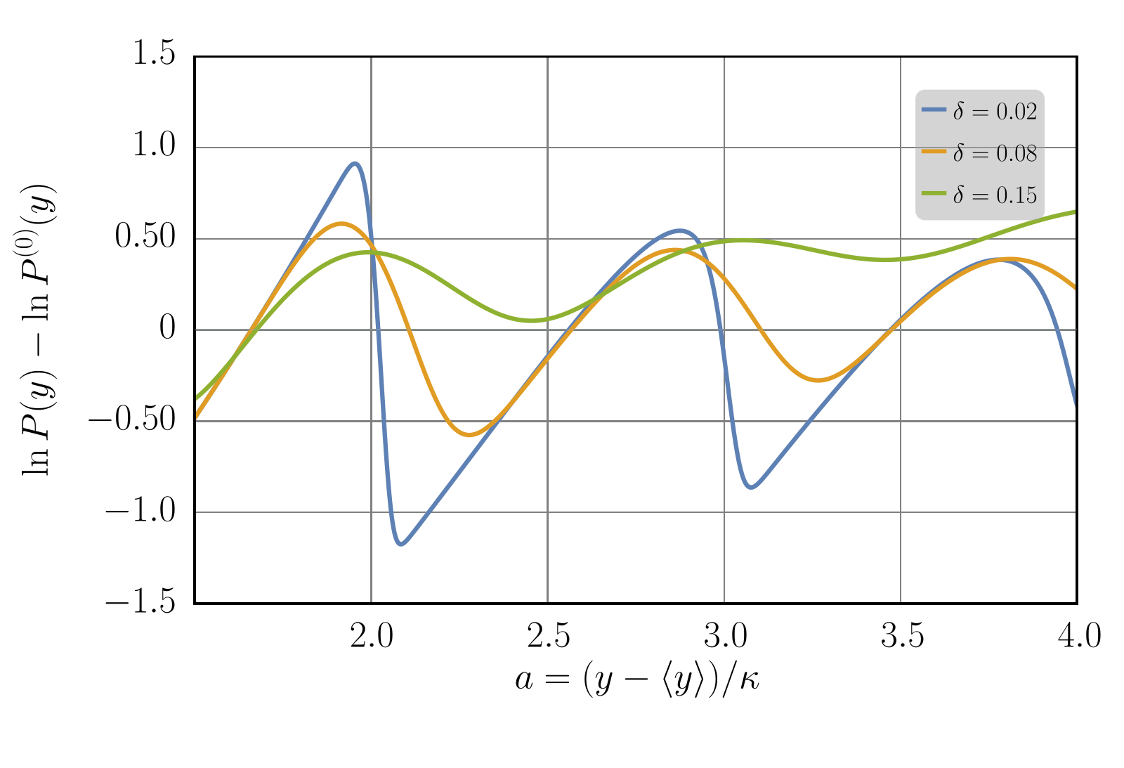
Figure G1: Plots of the logarithm of the multiplicative factor $f\left(y\right)$ distinguishing the leading asymptotic $P_{0}^{\left(0\right)}\left(y\right)$ behavior at large $y$ given by Eq. 220 (i. e. with $\delta=0$) and the true distribution of the dimensionless order parameter $P\left(y\right)=\exp\left\{f\left(y\right)\right\}\cdot P_{0}^{\left(0\right)}\left(y\right)$. On both plots, various curves correspond to various values of the standard deviation $\delta$ of the coupling matrix element. The argument is given by $a=\left(y-\left\langle y\right\rangle\right)/\kappa$. The microscopical parameters of the model are $\lambda\approx 0.12$, $Z=51$ and $\kappa\approx 5.0$. Left. The multiplicative correction estimated by the “model sum”  223, but with each term adjusted according to Eq. 342. Right. The plots for the multiplicative correction according to the direct numerical solution of the self-consistency equation 298 (solid lines) and the theoretical value for the PDF (dashed lines). The data from 6 was used, and discrepancies between the numerical and theoretical plots are also addressed under 6. The quantitative difference between the two plots is explained by the subleading corrections to the exponent of each term in Eq. 223 that are beyond the accuracy of the used expansions.

G.5.2 Fluctuating $Z$ model

Another simple yet informative model is the one that reproduces fluctuations of number of neighbors $Z$. Within this model, one chooses

$$P\left(c\right)=p\cdot\delta\left(1-c\right)+\left(1-p\right)\cdot\delta\left(c\right),\,\,\,\,0<p<1.$$ (343)

Each neighbor then has a fluctuating number of neighbors because each edge is either turned on with probability $p$, or turned off with probability $1-p$. The first moments of the actual number of neighbors are given by

$$\left\langle Z\right\rangle=pZ,\,\,\,\,\left\langle Z^{2}\right\rangle-\left\langle Z\right\rangle^{2}=Zp\left(1-p\right).$$ (344)

This simple model turns out to be very similar to the original model without the coupling disorder. Let us introduce the following renormalized values of the microscopical quantities:

$$\lambda_{R}=p\lambda,\,\,\,\,\,Z_{R}=pZ,\,\,\,\,\,\alpha_{R}=p\alpha,\,\,\,\,\,\kappa_{R}=\frac{\lambda_{R}}{\Delta_{0}Z_{R}},$$ (345)

where $\Delta_{0}$ is evaluated with the renormalized dimensionless Cooper constant $\lambda_{R}$, as described in G.1. Upon such renormalization, the equations on both $m_{1}$ and $m_{2}$ are exactly mapped on those for constant $Z$ presented in F:

$$m_{2}\left(S|w,x\right) =\lambda_{R}\cdot\intop_{0}^{1}dw_{1}\cdot\frac{\exp\left\{iS\kappa_{R}\eta\left(x\right)w_{1}\right\}-1-iS\kappa_{R}\eta\left(x\right)\cdot w_{1}}{w_{1}^{2}\sqrt{1-w_{1}^{2}}}$$

$$\times\left[1-w_{1}\left(1-w_{1}^{2}\right)\frac{\partial}{\partial w_{1}}\right]\cdot\left[\frac{\kappa_{R}w\eta\left(x\right)+m_{1}\left(w_{1},0\right)}{\kappa_{R}}\right],$$ (346)

$$m_{1}\left(w,x\right) =\eta\left(x\right)\cdot\lambda_{R}\intop_{0}^{1}dw_{1}\cdot\sqrt{1-w_{1}^{2}}\cdot\frac{m_{1}\left(w_{1},0\right)-m_{1}\left(0,0\right)}{w_{1}}$$

$$+\eta\left(x\right)\cdot\lambda_{R}\intop_{0}^{\infty}dy_{1}\cdot y_{1}\ln\frac{1}{y_{1}}\cdot\intop_{\mathbb{R}-i0}\frac{ds}{2\pi}\cdot\exp\left\{is\kappa_{R}\eta\left(x\right)w\right\}\cdot\exp\left\{m\left(s|0,0\right)-isy_{1}\right\}$$

$$+m_{1}\left(0,0\right)\cdot d\left(\Delta_{0}x\right)+\kappa_{R}w\left[\alpha_{R}\cdot\eta^{2}\left(x\right)+\lambda_{R}\cdot\psi\left(\Delta_{0}x\right)\right].$$ (347)

As a result, the sole effect of the fluctuation of the number of neighbors within such a model is pure renormalization of the microscopic parameters $\Delta_{0},\kappa,\lambda,\alpha$.