Smooth Sequential Optimisation with Delayed Feedback
Abstract.
Stochastic delays in feedback lead to unstable sequential learning using multi-armed bandits. Recently, empirical Bayesian shrinkage has been shown to improve reward estimation in bandit learning. Here, we propose a novel adaptation to shrinkage that estimates smoothed reward estimates from windowed cumulative inputs, to deal with incomplete knowledge from delayed feedback and non-stationary rewards. Using numerical simulations, we show that this adaptation retains the benefits of shrinkage, and improves the stability of reward estimation by more than 50%. Our proposal reduces variability in treatment allocations to the best arm by up to 3.8x, and improves statistical accuracy – with up to 8% improvement in true positive rates and 37% reduction in false positive rates. Together, these advantages enable control of the trade-off between speed and stability of adaptation, and facilitate human-in-the-loop sequential optimisation.
1. Introduction
Sequential adaptive optimisation is an example of a reinforcement learning system that progressively adapts the allocation of treatments in tune with the observed responses to these treatments. This methodology is typically framed as the classical multi-armed bandit problem of reward learning, and finds valuable applications in many domains, including clinical medicine (Press, 2009), political and social sciences (Imai and Strauss, 2011; Benartzi et al., 2017). It is also used for large-scale optimisation in the technology industry (Scott, 2010). In this context, it has improved the efficiency of online systems by automatically selecting better performing alternatives with minimal manual intervention. However, in many real-world applications of this technology, human operators are involved in higher-order decision making about generating treatment candidates, tuning optimisation goals, and tracking adaptation (Bakshy et al., 2018). To support such human-in-the-loop optimisation, the stability of adaptation is as important a goal as its efficiency. Smooth adaptation is naturally more interpretable, and enables human operators to conduct reliable hypothesis testing alongside the adaptation.
A particular challenge for achieving stable adaptation is delayed feedback. In many applications, stochastic delays in receiving feedback about treatments are common (Garg and Akash, 2019; Vernade et al., 2020). These delays can arise for various reasons – they can occur in actually administering the treatment once allocated, in measuring and communicating the response, and in the process of receiving and processing the response. Together, the additive consequence of such delays poses a challenge to the smoothness and stability of adaptation. The challenges posed by delayed feedback are further exacerbated when rewards are non-stationary, as is common in many practical scenarios. As we show, in these scenarios, maximum likelihood estimation (MLE) of rewards results in unstable learning behaviour, and makes hypothesis testing unreliable. The option of waiting until all the delayed feedback has been received is equally unattractive, as it would considerably slow down the pace of learning.
To help address this challenge, we propose computational improvements to recent applications of empirical Bayesian (eB) methods in this context (Dimmery et al., 2019). Compared to MLE, our improvements enable control of the trade-off between stability and speed of adaptation, supporting interpretable sequential optimisation. In addition to minimising regret, we improve the accuracy of hypothesis testing. Our novel contribution is an algorithmic adaptation of eB shrinkage estimation to learn from delayed feedback, such that
-
•
treatment allocations adapt smoothly to reward estimates that change due to delayed feedback and non-stationarity.
-
•
cumulative variance in estimation error is minimised in the long run.
-
•
statistical power of sequential Bayesian testing of hypotheses is maximised.
2. Related Work
2.1. Delayed Anonymous Feedback
We assume that individual responses to treatment allocations are generated by stochastic generative processes that govern both the response itself, and the delay in its generation. This follows the stochastic delayed composite anonymous feedback (SDCAF) model of bandit learning (Garg and Akash, 2019), which extends beyond previous work in this space (Pike-Burke et al., 2018; Cesa-Bianchi et al., 2018; Vernade et al., 2020). It assumes that responses are individually delayed and revealed at random points in the future. We extend this model to the batched online learning scenario, where we demonstrate the value of smooth empirical Bayesian shrinkage estimation.
2.2. Batched Bandit Learning
We combine the SDCAF model above with batch-based learning (Perchet et al., 2016). Batched learning extends the classic bandit problem to scenarios where a reinforcement learning agent pulls a batch of arms between consecutive learning updates. Batched learning has been well studied in the pure exploration setting, where the aim is to find the top-k arms as quickly as possible while minimising exploration cost, both in the absence (Jun et al., 2016) and presence (Grover et al., 2018) of delayed feedback.
Here, we focus on the online batched learning scenario, where the agent learns as it goes, both exploring and exploiting between consecutive updates. This is typical in the digital context (Scott, 2010), where individual responses are stored as they arrive and aggregated together anonymously to then update the agent, once per time interval between consecutive batched updates. We focus our analysis on the Thompson sampling agent (Agrawal and Goyal, 2012), which is well-suited to this scenario because of its stochastic allocation strategy. It pulls arms by sampling from Bayesian posterior distributions representing current knowledge of arm rewards. It updates this knowledge once per batch, by combining the individual responses received in that batch.
Combining batched online learning with the SDCAF model above, we allow the time interval between consecutive learning updates to be much shorter than the maximal time horizon allowed for the receipt of individually delayed responses, where is an integer number of consecutive updates. A natural consequence of this setup is that at every periodic update, the batch of data processed can include responses to treatment allocations “spilling over” from any of the batches in the past.
2.3. Empirical Bayesian Shrinkage
Empirical Bayesian estimation has been shown to be valuable for statistical learning at scale (Efron, 2011), and has recently been proposed for the batched, online sequential learning setting by Dimmery et al. (Dimmery et al., 2019). Specifically, the authors developed a novel application of James-Stein shrinkage to reduce reward estimation error in multi-armed bandits, and demonstrated its value for learning about the best set of arms. They showed that the benefit of eB for reward estimation grows with the number of arms. However, as they state, their formulation specifically assumes no “spillovers” of responses, hence avoiding the problem of delayed feedback.
Here, we extend Dimmery et al.’s work and augment eB estimation to account for the consequences of allowing such spillover generated by delays in responses. We draw upon research into empirical Bayesian smoothing (Shen and Lours, 1999; Maritz and Lwin, 2018), which has been employed to handle reporting delays in disease epidemiology (Meza, 2003; McGough et al., 2020), mirroring our delayed feedback context.
2.4. Bayesian Hypothesis Testing
Users of adaptive optimisation systems often also want to test hypotheses about statistically significant differences between arms, alongside achieving the core optimisation objective. However, the potential conflict between the primary reward optimisation goal needs to be balanced against the need for statistical power to achieve this secondary hypothesis testing goal. As a further novel contribution of this work, we address this need by combining eB optimisation with sequential hypothesis testing using Bayes factors (Schönbrodt et al., 2017). This framework combines bandit learning with Bayesian hypothesis testing to allow users to interrogate differences between arms, at any point during the sequential optimisation process.
3. Contribution
We develop smoothed eB models for bandit learning that account for delayed feedback and afford control over the trade-off between speed and stability of adaptation. To the best of our knowledge, the value of smoothed eB estimation has not been previously evaluated for enabling batched online learning with delayed feedback, in particular for enabling interpretability by supporting simultaneous hypothesis testing.
Here, we bring these aspects together in a novel algorithmic contribution detailed below. We focus on practical applications in the digital context, and complement existing theoretical work in this space with numerical simulations that replicate patterns of responses and delays observed in practice. We demonstrate that our contribution improves the recent proposal by Dimmery et al. (Dimmery et al., 2019) when handling delayed feedback, both in terms of stability of adaptive optimisation and hypothesis testing accuracy.
3.1. Shrinkage Estimation
Between consecutive updates of the learning agent, we randomly allocate individual treatment units to treatment arms , selecting from one of treatment arms, using Thompson sampling over reward distributions. As per the delayed feedback model above, at some future update , we observe the th unit’s response . Consequently, at each update , units have been allocated to arm , and responses have been observed, each of which have incurred a variable, stochastic delay.
At each update , we update our posterior reward distributions used for Thompson sampling. To perform this update, we employ shrinkage, a form of regularisation with many statistical benefits (Gelman et al., 2012). Specifically, we build upon the approach to shrinkage estimation proposed by Dimmery et al. (Dimmery et al., 2019), based on the James-Stein (JS) method (Efron, 2011). Specifically, to handle delayed feedback, we aggregate over recent treatment allocations and responses. Intuitively, our proposal makes the evolution of the posteriors more gradual over consecutive updates.
More formally, given allocations and responses at each batch, we calculate cumulative means and variances over treatment allocations and responses over most recent batches as
| (1) |
| (2) |
where are the variances of the reward estimates at batch . We then adapt Dimmery et al.’s formulation of the positive part JS estimator of each arm’s shrunk mean and variance , using the cumulative reward estimates:
| (3) |
| (4) |
where
| (5) |
and
| (6) |
The amount of shrinkage applied to each arm, , is calculated as:
| (7) |
With more data and lower cumulative variance , and/or larger differences in the cumulative means , approaches zero and eB estimation converges towards MLE.
3.2. Stability vs. Speed of Learning
Further, we control the stability vs. speed of convergence of treatment allocation by combining past shrunk estimates from recent updates. We calculate smoothed mean and variance over cumulative JS estimates and by combining recent updates:
| (8) |
| (9) |
where is a smoothing weight assigned to the JS estimate from update . The choice of allows control over the trade-off between speed and stability of convergence, as it allows us to control the influence of past estimates on the future ones. We develop alternatives for choosing that represent specific points along that trade-off. For example, setting
| (10) |
speeds up learning by only using the most recent JS estimate. However, this results in an unstable reinforcement learning loop, manifesting as oscillations in treatment allocations proportions from one update to the next, especially early in the learning process. This undesirable behaviour occurs because the delayed feedback model leads to spillover in the responses observed, causing alternating over- and under-estimation, even with shrinkage.
Alternatively, a uniform smoothing approach specified by assigns equal weights to recent JS estimates, thereby gaining smooth, stable allocation behaviour by averaging over the spillover, but at the cost of potentially underestimating rewards. A discounted smoothing approach specified by , linearly tapers the contribution of JS estimates based on their recency, affording a middle ground solution.
3.2.1. Stationary vs. Non-stationary Rewards
The benefits of smoothing can be extended by controlling , the length of the smoothing window. Setting to be equal to the total number of updates grows it linearly, producing asymptotic convergence, desirable under the assumption that true rewards are stationary. When they are non-stationary, and in particular piece-wise stationary, can be bounded to a sliding window over recent updates (Garivier and Moulines, 2008). This bounds the maximal delay to the length of the sliding window, converting the uniform and discounted smoothing alternatives described above to their non-stationary counterparts described by Garivier et al. (Garivier and Moulines, 2008).
3.3. Sequential Bayes Factors
Given a pair of arms, and , we evaluate the relative evidence for the hypotheses : that the true rewards of the arms are statistically indistinguishable and : that the true rewards of is greater than by at least a certain minimum detectable effect size.
At each update , we calculate this evidence in the form of sequential Bayes factors (Schönbrodt et al., 2017), which are interpreted as per (Kass and Raftery, 1995). Specifically, given the smoothed JS estimates defined as above, we calculate sequential Bayes factors (sBF) as
| (11) |
and can be initialised with prior expectations about the difference between the true rewards of and if available. If not, we initialise them with Gaussian noise priors (Dienes, 2014).
4. Simulations
We used numerical simulations to measure the performance of our smoothed eB alternatives to vanilla eB (Dimmery et al., 2019) and maximum likelihood estimation (MLE). We compared performance in three simulation contexts:
-
•
with synthetic arm rewards and response delays.
-
•
under stationary or non-stationary reward conditions.
-
•
with real rewards and delays observed at our company.
4.1. Synthetic Stationary Rewards
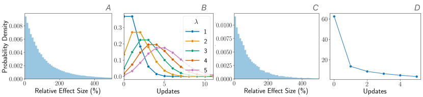
Each simulation consisted of 500 repeated trials. Each trial consisted of a sequence of 300 learning updates of the agent. At each such update , we allocated treatments to 1000 units and calculated smoothed estimates from the received responses. We assumed that true rewards were stationary, and hence, combined JS estimates from all updates between –. These JS estimates themselves are calculated from cumulative treatment allocations and responses between updates –. At the beginning of each trial, we created 15 treatment arms, with randomly initialised binary rewards , unknown to the learning agent. In synthetic simulations, we sampled from a beta distribution with parameters . Fig. 1A plots the distribution of true relative effect sizes, between all simulated arm pairs and across all trials.
We also randomly initialised each arm in a trial with a probabilistic delay also unknown to the agent, modelled as Poisson distributions with in –, illustrated in Fig. 1B. Given an arm with a randomly initialised delay , individual treatment responses generated by the arm would be stored in a buffer, and provided to the agent after a delay of updates. Hence, in a simulation run, arms would not only have unequal reward probabilities, they would also have unequal delays.
4.2. Synthetic Non-stationary Rewards
We simulated a simple non-stationary (piece-wise stationary) scenario where the true rewards are randomly interchanged at a single change point, by repeating the synthetic simulations above with two key differences:
4.3. Realistic Stationary Rewards
In realistic simulations, we instead sampled from distributions of real rewards and delays in treatment responses observed at our company. As Figs. 1C and 1D show, relative effect sizes and delays observed in reality were similar to the synthetic context.
In both synthetic and realistic simulations, we set the minimum detectable effect size to be . Across all simulation trials, approximately 55% of true differences between rewards were above this threshold, and were used to calculate the true positive rate, with the remaining used to calculate the false positive rate.
5. Results
We demonstrate improved stability of our two smoothed eB alternatives – eB with uniform smoothing (useB) and discounted smoothing (dseB) – when compared to vanilla eB without smoothing (veB (Dimmery et al., 2019)) and standard MLE without eB. We first report results from simulations with stationary synthetic rewards and delays, followed by non-stationary rewards. We then present results from simulations based on realistic rewards and delays observed at our company.
5.1. Treatment Allocation
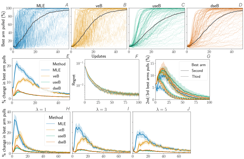
Fig. 2 compares the adaptation of treatment allocations, identifying relevant differences between the alternatives. Allocations adapted to the best arm in each trial, as function of how much better the best arm’s reward was, compared to the next best one. However, due to the impact of delayed feedback, both MLE and veB display unstable allocations to the best arm. In particular, this instability resulted in large oscillations that were especially prominent in the first 25 updates. In contrast, the smoothed variants of eB – useB and dseB – display a slower but stable pattern of adaptation that converges towards MLE with the reduction of shrinkage over updates. This observation is highlighted in Fig. 2E, which shows the average change (across trials) in allocation to the best arm from one update to the next. useB and dseB evidenced the most stable pattern of adaptation, facilitating better interpretation of system behaviour. Though veB was better than MLE, both were unstable across consecutive updates, with a max of 3.8x and 2.6x more instability relative to the smoothed eB alternatives, respectively. Though our approach to smoothing made adaptation to the best arm more stable, it did so without a major increase in overall regret in allocations, as shown in Fig. 2F.
Fig. 2G brings out a further aspect of our smooth eB alternatives. They spend more time, especially in early updates, exploring the second and third best arms more often. They adapt to allocate treatments to the best performing set of arms, rather than just the single best arm. In other words, they naturally manage the explore-exploit trade-off fundamental to reinforcement learning, without the need for a separate parameter. Importantly, as evident in the behaviour of the veB alternative, such exploratory behaviour is lost due to instabilities in delayed feedback. Hence, the smoothed alternatives we propose ‘recover’ this important advantage of eB.
5.1.1. Stability of adaptation as a function of delay
To provide further insights into how our proposals adapt to delayed feedback, we evaluated variability in treatment allocation to the best arm as function of the stochastic delay in receiving responses. We re-ran our simulations above, but now with the response-wise delay sampled from Poisson distribution with values of that were fixed at chosen values for the entire simulation run. Figs. 2H-J plot the average change in allocation to the best arm from one update to the next - the same as that plotted in Fig. 2E - but for specific values of . Reiterating the pattern in Fig. 2E, MLE and veB suffered higher instability in traffic allocation to the best arm. Further, this instability became more prolonged as the amount of delay increased. In comparison, useB and dseB showed consistent stability in allocation to the best arm, even under extended feedback delays generated when (see Fig 2J).
5.2. Reward Estimation
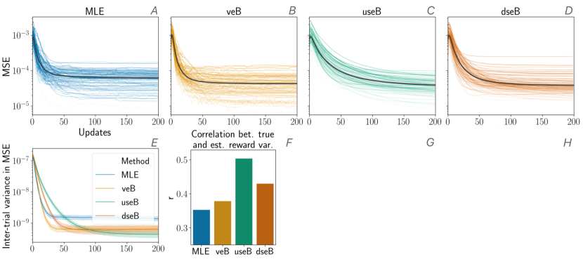
Delayed feedback causes observed rewards to oscillate, even if the true rewards are stationary. The advantages of our smoothed eB approaches are underpinned by improvements to reward estimation that are robust to this noise. This improvement can be seen in Figs. 3A-D. We observed lower variability in mean squared error (MSE) in reward estimation across arms with useB and dseB from one update to the next. This lower inter-update variability in reward estimation explains the lower variance in allocations to the best arms over consecutive updates (Fig. 2E).
Further, inter-trial variance in estimation error was also reduced in the longer term, see Fig. 3E. At the final update, this variance in estimation error was 52-69% lower with eB compared to MLE, between highlighting the general value of shrinkage. However, as can be seen in Fig. 3E, variance was initially higher with useB than MLE and veB, and less so with dseB, the middle ground option. This is to be expected, as early rewards being smoothed over are underestimates. This underestimation occurs because delays in receiving feedback mean that relatively few responses are received early on, but eventually start ‘piling up’. However, over subsequent updates, the value of smoothing becomes evident: the adverse effects of delays are accounted for, and inter-trial variability in reward estimation eventually stabilises at a lower level. Another insight into the behavior of our approach can be gained by measuring the across-trial correlation between the variance in true and estimated rewards, shown in fig, 3E. All eB methods, and smoothed eB methods more specifically, evinced an increased correlation. This correlation is also visually evident in the comparison of Figs. 3A-D, which confirms that, with our smoothed eB alternative in particular, MSE was higher in trials with a greater proportion of truly outlying rewards. This observation mirrors a point by Dimmery et al. (Dimmery et al., 2019), noting that eB approaches tend to be biased against outliers.
5.3. Hypothesis Testing
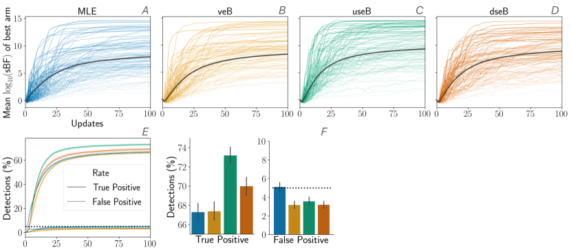
Yet another benefit of smoothing becomes evident when evaluating hypotheses about statistically significant differences between treatment arms. As Figs. 4A-D show, the average sequential Bayes factor of the best arm grows more consistently with useB and dseB. In turn, this leads to more accurate and better powered inferential statistics. To demonstrate this, we evaluated Type I and Type II errors by calculating true and false positive rates. Following the recommendation by Deng et al. (Deng et al., 2016), we specified an sBF threshold so as to guarantee a false discovery rate of no more than 5% with early stopping.
As shown in Fig. 4E, our useB and dseB alternatives achieved higher true positive rates and lower false positive rates. This is brought out clearly in Fig. 4F, which shows that, at the final update, true positive rates were 4-8% higher and false positive rates were 30-37% lower with the smoothed eB alternatives than with MLE. The underlying reason for this pattern becomes evident when considering how the smoothed alternatives modulate treatment allocation: because they allocate relatively more treatments to arms other than just the best one, they are better able to model the rewards of these other arms, and thereby significantly improve statistical power.
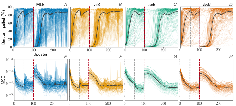
5.4. Non-stationary Rewards
As described above, delayed feedback causes observed rewards to evolve even if the true rewards themselves do not change. Non-stationarity in the true rewards further compounds the reward estimation problem. We examined a specific case of such non-stationarity where the true rewards are randomly interchanged mid-simulation, at update 100. The length of the smoothing window was bounded to 50 previous updates, to enable adaptation to this change (Garivier and Moulines, 2008). Fig. 5 depicts the adaptation of allocations to the best arm and MSE in this scenario. The change in arm rewards and the bounding of triggered significant ongoing instability in allocations to the best arm in the MLE and veB alternatives (Figs. 5A and 5B), underpinned by greater inter-update variability in reward estimation error (Figs. 5E and 5F). In comparison, useB and dseB evidenced slightly slower but much more stable adaptation in allocations (Figs. 5C and 5D), and much lower inter-update variability in estimation error (Figs. 5G and 5H). As highlighted previously, this speed vs. stability trade-off is controlled by the length and weighting of .
5.5. Real Rewards and Delays
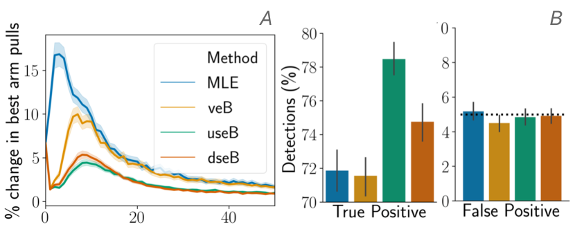
In this final section, we extend the generality and practical relevance of our results by demonstrating the performance of the smoothed eB alternatives in realistic simulations based on rewards and delays observed at our company (see Figs. 1B and 1C). As with the synthetic simulations, smoothed eB alternatives produced 1.8-2.8x lower peak variability in best arm pulls compared to MLE (compare Figs. 6A and 2E). Further, statistical accuracy was higher, with true positive rates 4-9% higher than MLE at the final update (compare Figs. 6B and 4F).
6. Conclusions
This paper has addressed practical challenges in modern adaptive optimisation. Stochastic delays and non-stationarity in feedback are a common phenomenon in online data streams, which necessarily complicate sequential reward estimation. We have proposed computationally lightweight augmentations that in effect, add a further layer of regularisation above empirical Bayesian estimation. The numerical simulations we conducted demonstrate the benefits realised when learning from delayed feedback, in the form of stable adaptation and estimation. These benefits become evident as adaptation progresses alongside changes in true rewards.
We speculate that the benefits our proposal will become more prominent with further increases in the amount and skew in feedback delays, e.g., when treatments include multiple interventions before a response can be generated. Further, there are likely to be other scenarios where it would be valuable. For example, when there are arm-wise asymmetries in the cost of misallocation of treatments. Yet another scenario involves learning with privatised data, where the addition of differential privacy noise could adversely impact accurate reward estimation.
Further, our proposal also benefits the complementary desire for hypothesis testing. This feature is often an important part of human-in-the-loop optimisation (Bakshy et al., 2018), assisting human controllers in higher-order decision making that is informed by statistically robust inference. Strictly speaking, focusing only on maximising overall reward with adaptive allocation can conflict with reliable hypothesis testing, as few, if any, treatments would be allocated to weaker arms. However, as we show, smoothed empirical Bayesian estimation achieves a balance between these objectives – not only does it stabilise adaptation with similar regret, it also improves Type I and Type II error rates.
References
- (1)
- Agrawal and Goyal (2012) Shipra Agrawal and Navin Goyal. 2012. Analysis of thompson sampling for the multi-armed bandit problem. In Journal of Machine Learning Research, Vol. 23. 39–40. http://proceedings.mlr.press/v23/agrawal12/agrawal12.pdf
- Bakshy et al. (2018) Eytan Bakshy, Lili Dworkin, Brian Karrer, Konstantin Kashin, Benjamin Letham, Ashwin Murthy, and Shaun Singh. 2018. AE: A domain-agnostic platform for adaptive experimentation. Conference on Neural Information Processing Systems Nips (2018), 1–8. http://eytan.github.io/papers/ae_workshop.pdf
- Benartzi et al. (2017) Shlomo Benartzi, John Beshears, Katherine L Milkman, Cass R Sunstein, Richard H Thaler, Maya Shankar, Will Tucker-Ray, William J Congdon, and Steven Galing. 2017. Should Governments Invest More in Nudging? Psychological Science 28, 8 (2017), 1041–1055. https://doi.org/10.1177/0956797617702501
- Cesa-Bianchi et al. (2018) Nicolò Cesa-Bianchi, Yishay Mansour, Sebastien Bubeck, Vianney Perchet, and Philippe Rigollet. 2018. Nonstochastic Bandits with Composite Anonymous Feedback. In Proceedings of Machine Learning Research, Vol. 75. 1–23. http://proceedings.mlr.press/v75/cesa-bianchi18a/cesa-bianchi18a.pdf
- Deng et al. (2016) Alex Deng, Jiannan Lu, and Shouyuan Chen. 2016. Continuous monitoring of A/B tests without pain: Optional stopping in Bayesian testing. In Proceedings - 3rd IEEE International Conference on Data Science and Advanced Analytics, DSAA 2016. 243–252. https://doi.org/10.1109/DSAA.2016.33
- Dienes (2014) Zoltan Dienes. 2014. Using Bayes to get the most out of non-significant results. Frontiers in Psychology 5, July (2014), 1–17. https://doi.org/10.3389/fpsyg.2014.00781
- Dimmery et al. (2019) Drew Dimmery, Eytan Bakshy, and Jasjeet Sehkon. 2019. Shrinkage estimators in online experiments. In Proceedings of the ACM SIGKDD International Conference on Knowledge Discovery and Data Mining. 2914–2922. https://doi.org/10.1145/3292500.3330771
- Efron (2011) Bradley Efron. 2011. Large-Scale Inference: Empirical Bayes Methods for Estimation, Testing, and Prediction. International Statistical Review 79, 1 (2011), 126–127. https://doi.org/10.1111/j.1751-5823.2011.00134{_}13.x
- Garg and Akash (2019) Siddhant Garg and Aditya Kumar Akash. 2019. Stochastic Bandits with Delayed Composite Anonymous Feedback. https://arxiv.org/pdf/1910.01161.pdfhttp://arxiv.org/abs/1910.01161
- Garivier and Moulines (2008) Aurélien Garivier and Eric Moulines. 2008. On Upper-Confidence Bound Policies for Non-Stationary Bandit Problems. (2008). https://arxiv.org/pdf/0805.3415.pdf
- Gelman et al. (2012) Andrew Gelman, Jennifer Hill, and Masanao Yajima. 2012. Why We (Usually) Don’t Have to Worry About Multiple Comparisons. Journal of Research on Educational Effectiveness 5, 2 (2012), 189–211. https://doi.org/10.1080/19345747.2011.618213
- Grover et al. (2018) Aditya Grover, Todor Markov, Peter Attia, Norman Jin, Nicholas Perkins, Bryan Cheong, Michael Chen, Zi Yang, Stephen Harris, William Chueh, and Stefano Ermon. 2018. Best arm identification in multi-armed bandits with delayed feedback. In International Conference on Artificial Intelligence and Statistics, AISTATS 2018. 833–842. http://proceedings.mlr.press/v84/grover18b/grover18b.pdf
- Imai and Strauss (2011) Kosuke Imai and Aaron Strauss. 2011. Estimation of heterogeneous treatment effects from randomized experiments, with application to the optimal planning of the get-out-the-vote campaign. Political Analysis 19, 1 (2011), 1–19. https://doi.org/10.1093/pan/mpq035
- Jun et al. (2016) Kwang Sung Jun, Kevin Jamieson, Robert Nowak, and Xiaojin Zhu. 2016. Top arm identification in multi-armed bandits with batch arm pulls. In Proceedings of the 19th International Conference on Artificial Intelligence and Statistics, AISTATS 2016. 139–148. http://proceedings.mlr.press/v51/jun16.pdf
- Kass and Raftery (1995) Robert E Kass and Adrian E Raftery. 1995. Bayes Factors. J. Amer. Statist. Assoc. 90, 430 (1995), 319–323. https://doi.org/10.1080/01621459.1995.10476572
- Maritz and Lwin (2018) J. S. Maritz and T. Lwin. 2018. Empirical bayes methods, second edition. Chapman and Hall/CRC. 1–284 pages. https://doi.org/10.1201/9781351071666
- McGough et al. (2020) Sarah F. McGough, Michael A. Johansson, Marc Lipsitch, and Nicolas A. Menzies. 2020. Nowcasting by Bayesian smoothing: A flexible, generalizable model for real-time epidemic tracking. PLoS Computational Biology 16, 4 (4 2020), e1007735. https://doi.org/10.1371/journal.pcbi.1007735
- Meza (2003) Jane L. Meza. 2003. Empirical Bayes estimation smoothing of relative risks in disease mapping. Journal of Statistical Planning and Inference 112, 1-2 (3 2003), 43–62. https://doi.org/10.1016/S0378-3758(02)00322-1
- Perchet et al. (2016) Vianney Perchet, Philippe Rigollet, Sylvain Chassang, and Erik Snowberg. 2016. Batched bandit problems. Annals of Statistics 44, 2 (2016), 660–681. https://doi.org/10.1214/15-AOS1381
- Pike-Burke et al. (2018) Ciara Pike-Burke, Shipra Agrawal, Csaba Szepesvári, and Steffen Grünewälder. 2018. Bandits with delayed, aggregated anonymous feedback. In 35th International Conference on Machine Learning, ICML 2018, Vol. 9. 6533–6574. https://arxiv.org/pdf/1709.06853.pdf
- Press (2009) William H Press. 2009. Bandit solutions provide unified ethical models for randomized clinical trials and comparative effectiveness research. Proceedings of the National Academy of Sciences of the United States of America 106, 52 (2009), 22387–22392. https://doi.org/10.1073/pnas.0912378106
- Schönbrodt et al. (2017) Felix D Schönbrodt, Eric Jan Wagenmakers, Michael Zehetleitner, and Marco Perugini. 2017. Sequential hypothesis testing with Bayes factors: Efficiently testing mean differences. Psychological Methods 22, 2 (2017), 322–339. https://doi.org/10.1037/met0000061
- Scott (2010) Steven L Scott. 2010. A modern Bayesian look at the multi-armed bandit. Applied Stochastic Models in Business and Industry 26, 6 (2010), 639–658. https://doi.org/10.1002/asmb.874
- Shen and Lours (1999) Wei Shen and Thomas A. Lours. 1999. Empirical Bayes Estimation via the Smoothing by Roughening Approach. Journal of Computational and Graphical Statistics 8, 4 (12 1999), 800–823. https://doi.org/10.1080/10618600.1999.10474850
- Vernade et al. (2020) Claire Vernade, Alexandra Carpentier, Tor Lattimore, Giovanni Zappella, Beyza Ermis, and Michael Brueckner. 2020. Linear Bandits with Stochastic Delayed Feedback. In Proceedings of the 37th International Conference on Machine Learning. http://proceedings.mlr.press/v119/vernade20a/vernade20a.pdf