Searches for beyond-Riemann gravity
Abstract
Many effective field theories describing gravity cannot arise from an underlying theory based on Riemann geometry or its extensions to include torsion and nonmetricity but may instead emerge from another geometry or may have a nongeometric basis. The Lagrange density for a broad class of such theories is investigated. The action for fermions coupled to gravity is linearized about a Minkowski background and is found to include terms describing small deviations from Lorentz invariance and gravitational gauge invariance. The corresponding nonrelativistic hamiltonian is derived at second order in the fermion momentum. The implications for laboratory experiments and astrophysical observations with fermions are studied, with primary focus on anomalous spin-gravity couplings. First constraints on some coefficients are extracted from existing data obtained via measurements at different potentials, comparisons of gravitational accelerations, interferometric methods, and investigations of gravitational bound states. Some prospects for future experimental studies are discussed.
I Introduction
The construction of a compelling and realistic underlying theory that unifies gravity with quantum physics remains an open challenge. The description of spacetime in the underlying theory might involve the usual Riemann geometry of General Relativity (GR), or it might be a non-Riemann geometry or have no geometrical basis. An interesting and potentially vital issue is then the extent to which current or feasible experiments can help to distinguish between these possibilities.
Coupling GR to the Standard Model (SM) of particle physics produces a theory that is quantum incomplete but that yields an excellent match to experiments in suitable regimes. Any deviations from known physics emerging from the underlying unified theory are therefore expected to be small, perhaps suppressed by a large scale such as the Planck mass. A model-independent approach to studying small deviations from a known theory is provided by effective field theory (EFT) sw09 . Investigations of the geometric properties of the underlying unified theory can therefore be based on the general EFT constructed from the action of GR coupled to the SM.
To allow for deviations from Riemann geometry, the general EFT must contain both terms preserving and violating the spacetime symmetries of GR, which include the invariances under local Lorentz transformations and diffeomorphisms. The general EFT based on GR coupled to the SM is presented in Ref. ak04 . Each additional term in the action involves a coupling coefficient combined with an operator constructed from dynamical fields. A given coupling coefficient can be viewed as a background that can carry spacetime or local indices and can depend on spacetime position. Except for the special case of a constant scalar coupling, any coefficient controls violations of one ore more of the invariances of GR. The coefficients can also be flavor dependent, so violations of the weak equivalence principle (WEP) are incorporated. A given term in the EFT action can be classified according to the mass dimension of the dynamical operator it contains, with minimal terms defined to have and nonminimal ones . A systematic construction of all terms has recently been presented in Ref. kl21 .
The background coefficients can be dynamical or prescribed quantities. In the former case they are called spontaneous, and in the latter explicit. At the EFT level, a spontaneous background consists of a vacuum value solving the equations of motion, together with dynamical fluctuations about that include Nambu-Goldstone and massive modes. In contrast, an explicit background is a predetermined quantity. The presence of the fluctuations generates corresponding physical effects, which can distinguish a spontaneous background from an explicit background . In the present work, we focus primarily on EFT based on GR coupled to the SM and containing one or more explicit backgrounds .
The structure of an EFT with an explicit background can be constrained by the requirement of compatibility between the variational procedure and the Bianchi identities of Riemann geometry ak04 ; rb15 ; kl21 . It turns out that most EFT terms with explicit backgrounds are perturbatively incompatible with Riemann geometry or its extensions with torsion and nonmetricity, and hence typical models containing terms of this type must be based on a different geometry or have a nongeometric origin. These no-go constraints provide a powerful tool to specify terms that cannot arise in Riemann geometry and thereby to identify physical effects serving as experimental signals for an underlying unified theory based on nonstandard geometry or on a nongeometrical structure.
In the present work, we explore this line of reasoning by investigating physical effects in a large class of EFT based on GR coupled to the SM and incorporating terms that involve beyond-Riemann effects. For this initial study, we focus on gravitational couplings of fermions and in particular spin-gravity couplings, which have implications for many existing laboratory and astrophysical observations. We consider in turn experiments involving measurements at different potentials, comparisons of gravitational accelerations, interferometric methods, and gravitational bound states. We use existing experimental data to obtain first constraints on the EFT coefficients governing beyond-Riemann physics. We also discuss prospects for some future experimental studies.
The organization of this paper is as follows. The setup for the EFT containing beyond-Riemann effects is presented in Sec. II. We provide tables detailing the terms in the action and their linearizations. The corresponding nonrelativistic hamiltonian is obtained, and its coefficients are related to those in the linearized Lagrange density. The flavor dependence of the coefficients corresponding to WEP violations is discussed, including implications for antiparticles. This material makes feasible the analysis of various experiments. In Sec. III we adopt results from existing experiments performed at different potentials to extract first constraints on some coefficients in the EFT. Another class of experiments, analyzed in Sec. IV, involves comparing the gravitational accelerations of different atoms. We consider tests with Sr atoms of different spins and with Rb atoms in different hyperfine states, and we discuss the prospects for comparing the gravitational accelerations of matter and antimatter. In Sec. V, we turn attention to interferometric experiments with neutrons to obtain sensitivity to additional coefficients. Studies of neutrons bound in the Earth’s gravitational field can also provide interesting measurements and are treated in Sec. VI. We summarize our results in Sec. VII.
Throughout this work, we follow the conventions of Ref. kl21 , using natural units with . For the experimental analyses, we adopt standard reference frames widely used in the literature. No laboratory on the Earth lies in an inertial frame, so experimental results for coefficients are reported in the canonical Sun-centered frame sunframe . This right-handed orthogonal system has spatial coordinates , with the axis aligned along the Earth’s rotation axis and with the axis pointing from the Earth to the Sun at the vernal equinox 2000, which serves as the zero of the time . For some calculations, it is convenient to adopt a canonical laboratory frame having time coordinate and spatial coordinates , with the axis oriented toward the local zenith sunframe . Neglecting the Earth’s boost, the transformation from the Sun-centered frame to the canonical laboratory frame is given by the rotation matrix
| (1) |
where is the laboratory colatitude, is the sidereal frequency of the Earth’s rotation, and is a suitable local sidereal time. In what follows, some expressions involve coefficients with indices either summed over , , , and denoted for brevity by the pair , or summed over , , , and denoted by the pair .
II Theory
One goal of this work is to construct an EFT based on GR coupled to the SM that contains a general class of terms excluded in Riemann geometry. This provides a window on physics effects from beyond-Riemann theories and permits the extraction of experimental constraints. Here, we focus specifically on fermion-gravity couplings, which are ubiquitous and comparatively straightforward to analyze for most laboratory experiments and astrophysical observations, while maintaining a broad and model-independent perspective.
Our primary interest lies in spin-gravity couplings, in part because they are particularly challenging to fit into Riemann geometry kl21 , but in this section we include effects from spin-independent terms as well. The methodology presented here could therefore be applied to measurements of spin-independent fermion-gravity couplings, including precision experiments associated with WEP tests ti20 . Both spin-dependent and spin-independent fermion-gravity couplings are known to arise in beyond-Riemann contexts. In Finsler geometry rf ; bcs00 , for example, the metric is supplemented with objects on the manifold that have been conjectured to play the role of the explicit backgrounds in generic EFT based on GR coupled to the SM ak04 . Although a complete demonstration of this link awaits the resolution of open issues in Lorentz-Finsler geometry ak11 ; bjs20 ; ps18 ; em17 ; tbgm18 ; ilp18 ; cs18 ; rt18 ; xl18 ; sma19 ; sv20 ; rl20 ; fhpv20 , the resulting trajectories arising from spin-gravity couplings in a fixed gravitational background are known to correspond to Riemann-Finsler geodesics ak11 ; ms19 ; dc17 ; fl15 ; nr15 . Possible gravitational couplings to boson fields, including photons, are also of definite interest but lie beyond our present scope.
II.1 Setup
In theories with a geometric foundation, the equations of motion obtained from the variational principle are supplemented by geometric conditions called the Bianchi identities, which arise from the structure of the corresponding fiber bundle mtw . For many geometric theories, such as Maxwell electrodynamics or other gauge theories in Minkowski spacetime, the Bianchi identities are homogeneous equations that are independent of the inhomogeneous equations generated via the variational procedure. In contrast, in some geometric theories such as GR, the equations of motion are entangled with the geometry. The Bianchi identities then impose a self-consistency condition, which for GR turns out to be the requirement of covariant conservation of the energy-momentum tensor. This is compatible with the matter equations of motion, so GR is self consistent. However, for some theories the geometric conditions can be incompatible with the results of the variational principle and hence serve as no-go constraints ak04 .
This issue is of particular relevance for theories that purport to be based on Riemann geometry but that violate spacetime symmetries. The geometric constraints become particularly stringent for theories required to produce only perturbative corrections to GR at low energies while also maintaining the structure of Riemann geometry. Indeed, most theories of this type with explicit breaking of spacetime symmetries are incompatible with Riemann geometry ak04 . Many examples illustrating the no-go constraints are known ak04 ; kl21 ; rb15 . The simplest may be the extension of GR containing a cosmological term that involves a prescribed nontrivial function of spacetime position rb15 , resulting in explicit diffeomorphism violation (EDV). Variation of the action yields Einstein equations taking the usual form, but these are incompatible with the Bianchi identities unless is a spacetime constant, which contradicts the initial assumption. A recent general discussion of the no-go constraints along with other examples is given in Sec. II F of Ref. kl21 .
The present work is based on the above results. We take advantage of the potential incompatibility between the Bianchi identities and the variation of the action to investigate a large class of possible underlying theories that have a non-Riemann geometry or a nongeometric basis while nonetheless reducing at low energies to a perturbatively corrected version of GR coupled to the SM. The perturbative nature implies that this class of theories can naturally be studied in the EFT framework sw09 . A typical application of the framework would involve constructing a specific EFT based on integrating over high-energy degrees of freedom in a theory and ensuring self-consistency via loops. Here, however, we adopt a different approach, designed instead to study simultaneously a large class of theories with a given symmetry structure and to investigate their possible phenomenological EFT signatures. The approach involves constructing all EFT operators compatible with the specified symmetry and comparing their effects to experimental data. This yields bounds that restrict the viability of members of the class, thereby providing guidance on the acceptability of underlying models. The technique is appropriate and powerful in situations where no experimental evidence exists for the effects being sought, as is the case here. For spacetime-symmetry violations, this EFT approach was developed in Ref. kp95 to study spontaneous Lorentz violation in string theory ksp . It was subsequently applied to the SM to yield the Standard-Model Extension (SME) in Ref. ck97 and generalized to GR coupled to the SM in Ref. ak04 .
Our focus here is on perturbations to GR coupled to the SM involving EFT terms that have EDV while maintaining local Lorentz invariance (LLI). The perturbative nature and the EDV imply incompatibility between the equations of motion and the Bianchi identities of Riemann geometry ak04 ; kl21 , so these terms can be attributed to models within a class of beyond-Riemann theories. The LLI-EDV symmetry structure is of particular interest because the corresponding EFT terms lack the severe phenomenological complications from additional modes that typically arise in theories with explicit breaking. As a result, EFT operators can be constructed explicitly for this class of theories and can be constrained using experimental and observational data. The latter is the primary goal of the present work.
Details of the framework for the EFT construction have been presented in Refs. ak04 ; kl21 and involve several complications, notably the appearance of additional physical modes beyond those arising in GR coupled to the SM. The role of these additional modes can be reduced by eliminating terms controlling their propagation, which removes effects of extra long-range forces. One set of such modes is the antisymmetric tensor associated with local Lorentz violation. To avoid these modes, we restrict the EFT to preserve LLI, which insures that contains only unphysical gauge degrees of freedom. The other set of additional modes is the vector associated with diffeomorphism violation. To incorporate beyond-Riemann effects when LLI holds, EDV must be present. The resulting modes have physical effects, but their free propagation can be avoided by taking the pure-gravity sector to be conventional rb15 . The modes can then be viewed as nonpropagating auxiliary fields with derivative couplings in the matter-gravity sector of the EFT. To simplify the analysis here, we assume dynamical torsion and nonmetricity are absent. However, the present EFT framework applies also to phenomenological and experimental studies of fermion couplings involving explicit background torsion torsion and nonmetricity nonmetricity .
The laboratory experiments and astrophysical observations considered here involve comparatively weak gravitational fields, so the linearized limit is sufficient for a phenomenological analysis of dominant effects from the EFT. In the linearized EFT, the local Lorentz and diffeomorphism transformations combine to yield Lorentz, gauge, and translation transformations acting in approximately Minkowski spacetime kl21 . For simplicity, we can limit attention to linearized terms that maintain translation invariance (TI). All such terms exhibit either Lorentz invariance (LI) or Lorentz violation (LV), and either gauge invariance (GI) or gauge violation (GV).
We remark in passing that the above choices for the EFT can be matched to the classification presented in Table IV of Ref. kl21 . In this language, the present work limits attention to EFT terms lying both in the row labeled LLI, EDV and in the columns labeled LI-GI-TI, LV-GV-TI, LI-GV-TI, and LV-GI-TI. These terms all generically violate the no-go constraints because they are perturbatively incompatible with the Bianchi identities of Riemann geometry. In the context of Fig. 2 of Ref. kl21 , the EFT we consider lies in the lower left triangle of the hexagon, labeled LLI, EDV.
| Component | Expression |
|---|---|
For our phenomenological analyses, we focus on leading-order effects arising from the propagation of a Dirac fermion of mass in the presence of a weak gravitational field with metric . The metric fluctuation includes contributions from the derivatives of the modes. Note, however, that in the EFT context these contributions are determined by the backgrounds and represent small corrections to the GR value of . The weak-field assumption implies that the latter is already small, so for many applications can be approximated at leading order by its GR value. For simplicity, we neglect possible couplings to derivatives of the backgrounds . It then suffices to consider quadratic fermion terms and their gravitational couplings, allowing for arbitrary LLI-EDV operators. All the relevant fermion-gravity terms involving operators with and without background derivatives are presented in Table XI of Ref. kl21 . As increases, these terms acquire more fermion derivatives and hence can be expected to generate suppressed effects in laboratory experiments because the relevant fermion momenta are small compared to the Planck scale. Nonetheless, to capture effects from both minimal and nonminimal terms, the analysis that follows includes terms containing operators with .
Implementing the linearization to extract all fermion terms with operators of mass dimension in the Lagrange density of the linearized EFT, we find the results displayed in Table 1. In the table, is separated into pieces containing terms with specified and number of derivatives of . These pieces are listed in the first column, while the second column shows the explicit form of the corresponding terms. The first two rows in the table represent the linearization of the usual Lagrange density for a massive Dirac fermion coupled to gravity, and they lie in the LI-GI-TI class. All other terms in the table exhibit LV, GV or both. The only LI terms are ones with coefficients constructed from the Minkowski metric and the Levi-Civita tensor . The only GI terms involve combinations of two derivatives of the metric fluctuation that arise from the curvature tensor. The notation for each coefficient appearing in the table is chosen in accordance with standard usage in the literature, with a superscript L indicating that the corresponding operator is linearized. The primary letter on a coefficient distinguishes the spin and charge-conjugation, parity-inversion, and time-reversal (CPT) properties of the dynamical operator, while the subscript indicates the number of derivatives of it contains.
The terms listed in Table 1 are obtained by linearization of the full fermion-gravity Lagrange density provided in Table XI of Ref. kl21 . The coefficients appearing in Table 1 are therefore combinations of relevant parts of the breve coefficients appearing in Table XI of Ref. kl21 . Each breve coefficient is a linear combination of backgrounds contracted with vierbeins, metrics, and Levi-Civita tensors. In the linearized scenario relevant to the EFT of interest here, a generic breve coefficient can be written as a sum of two parts involving explicit backgrounds,
| (2) | |||||
where the background appearing in the approximately Minkowski spacetime is the breve coefficient taken at zeroth order in vierbein and metric fluctuations,
| (3) |
For example, the breve coefficient appearing in the piece of reduces in the present EFT context to , with and . Note that our assumption of TI for the linearized theory implies that all coefficients considered here are spacetime constants.
The explicit relationships between the linearized coefficients appearing in Table 1 and the breve coefficients appearing in are provided in Table 2. The first column of this table displays the linearized coefficients appearing in , while the second column establishes the link to the explicit backgrounds contained in the breve coefficients appearing in and defined via Eq. (2). Note that the asymptotic parts of certain breve coefficients are absent in Table 2 because they contribute to the linearized EFT only for .
II.2 Nonrelativistic hamiltonian
The linearized Lagrange density given in Table 1 can be used as the basis for phenomenological analyses. However, many laboratory experiments sensitive to fermion-gravity couplings involve slow-moving particle species experiencing the gravitational field of the Earth. For these types of experiments, the analysis of data for signals of physics beyond Riemann gravity involves the nonrelativistic particle hamiltonian . This can be extracted from the linearized Lagrange density via a generalized Foldy-Wouthuysen transformation fw50 , using techniques established for backgrounds violating spacetime symmetries kl99jmp ; kl01 ; gos09 ; kt11 ; km12 ; km13 ; yb13 ; cl16 ; zx18 .
At leading order in the backgrounds, the perturbative relativistic hamiltonian can be identified from the Euler-Lagrange equations obtained by variation of the linearized action km12 . In approximately flat spacetime, this bypasses the complications of nonstandard time evolution introduced by certain background components and hence avoids the necessity for prior field redefinitions kt11 or modifications to the inner product in the Hilbert space lp80 . The relativistic hamiltonian can then be block diagonalized at the desired order in the particle 3-momentum using an iterative method, and the nonrelativistic hamiltonian can be extracted from the upper block kl99jmp . The results obtained via this procedure generalize those in Ref. km13 obtained for a Dirac fermion in Minkowski spacetime in the presence of Lorentz-violating operators of arbitrary mass dimension .
With the above techniques, the derivation of the nonrelativistic hamiltonian from the linearized Lagrange density in Table 1 is lengthy but straightforward. It is convenient to express the result as a sum of pieces,
| (4) |
where is the hamiltonian in the absence of backgrounds. In this sum, the spin-dependent terms containing the Pauli spin matrices are identified with a subscript . The perturbative corrections of this type represent anomalous spin-gravity couplings and in this context can be viewed as WEP violations. The pieces with a subscript depend directly on the gravitational potential , while those with a subscript depend only on the gravitational acceleration . The ellipsis indicates terms that depend on higher derivatives of .
For applications to laboratory experiments, it typically suffices to take the gravitational acceleration in the laboratory as uniform and directed along in the canonical laboratory frame, , so the gravitational potential is . We incorporate here relativistic corrections to second order in . With these approximations, we can extract explicit forms for the various terms in the hamiltonian (4).
For the piece , the procedure generates the expression
| (5) |
The first two terms on the right-hand side are the usual strict nonrelativistic limit. The third term is the leading-order relativistic correction, while the last term is the spin-orbit coupling. Note that no Darwin-type term proportional to the divergence of appears because is uniform by assumption. The form of has been the subject of numerous investigations in the literature ot62 ; as78 ; ffc81 ; hn90 ; cp91 ; jh94 ; vr00 ; yo01 ; st05 . Our result (5) matches Eq. (14) in Ref. st05 , which was derived for uniform acceleration and expressed in the physical Foldy-Wouthuysen representation.
The spin-independent piece of coupling via the gravitational potential can be written in the form
| (6) | |||||
where the coefficient is defined to be symmetric,
| (7) |
Each term in Eq. (6) depends on position through the dependence on the gravitational potential. The coefficients , , and are spacetime constants that control the magnitude of the effects produced by the operators in . The superscripts NR serve as a reminder that the coefficients are defined in the nonrelativistic limit, while the subscripts and reflect the dependence on the potential and on the fermion momentum. The term with coefficient and the component of the third term governed by the trace of are invariant under rotations, and they represent EFT contributions that shift the sizes of the second and third terms in . The remaining terms in violate rotation symmetry. The term in with coefficient violates parity P and time reversal T, while the other two are P and T even.
The spin-dependent piece of coupling via the gravitational potential is given by
| (8) | |||||
In this equation, the coefficient is defined to be symmetric on the last two indices,
| (9) |
and all the coefficients are spacetime constants. Each term in inherits dependence on the position from the gravitational potential. The second term contains a rotation-invariant component controlled by the trace . The corresponding operator represents rotation-invariant effects that are distinct from those appearing in the hamiltonian with vanishing backgrounds. The component of proportional to is absent in because the corresponding operator vanishes identically. The first and third terms in are P even and T odd, while the second term is P odd and T even.
Turning next to the pieces of coupling via the gravitational acceleration , we find that the spin-independent piece can be written in the form
| (10) |
where we define
| (11) |
All three terms in the expression (10) are position independent. All are rotation violating, except for the operator in the second term associated with the trace . Note that in principle a totally antisymmetric component of would govern rotation-invariant effects, but the corresponding operator vanishes identically. The second term in is P even and T odd, while the other two are P odd and T even.
| NR coefficient | Linearized coefficient |
|---|---|
Finally, the spin-dependent terms coupling with the gravitational acceleration are found to be
| (12) | |||||
where we define
| (13) |
The three terms in Eq. (12) are all position independent. Each term contains a rotation-invariant component. The first involves the dipole spin-gravity operator , governed by the trace . In the absence of backgrounds, the possible appearance of this operator in the hamiltonian has been the subject of discussion in the literature yo01 , but it is known to be absent when the physical Foldy-Wouthuysen representation is adopted st05 . Here, despite the use of this representation, the dipole spin-gravity operator nonetheless appears because the general EFT provides additional contributions to , so its detection would represent a signal of new physics. Note that the third term in incorporates a rotation-invariant component , which corrects the dipole spin-gravity coupling at , along with another rotation scalar . The second term also contains a rotation scalar associated with the component proportional to , which acts to correct the size of the last term in . The first and third terms in are P and T odd, while the second is P and T even.
It is useful to collect all the rotation-invariant contributions to , which gives
| (14) | |||||
where the correction terms are ordered by increasing powers of the 3-momentum. The coefficients with primes denote suitably normalized irreducible representations of the rotation group obtained from the nonrelativistic coefficients in Eqs. (6)–(12). The expression (14) for is of interest for certain experimental applications, in part because the rotation invariance ensures that all terms take the same form at leading order when expressed either in the laboratory frame or the Sun-centered frame. This implies, for example, no leading-order dependence on the local sidereal time or laboratory colatitude in experimental signals for these terms. Note, however, that can be modified by boosts, including the boost associated with the revolution of the Earth about the Sun. Note also that some of the rotation-invariant terms (14) have been proposed in other contexts as phenomenological modifications to conventional fermion-gravity couplings lo64 ; ni10 . The present work reveals how these and other effects can arise in the EFT context.
The expressions (5), (6), (8), (10), and (12) are derived for the special gravitational potential associated with a uniform gravitational field . The nonrelativistic coefficients appearing in these expressions are therefore strictly defined only in this restricted scenario, which makes challenging direct comparisons of their measurements with results from other types of laboratory experiments and astrophysical observations. It is therefore crucial to report the results of any given data analysis also as measurements of coefficients in the linearized Lagrange density in Table 1.
The explicit relationships between coefficients in the nonrelativistic hamiltonian and coefficients in the linearized Lagrange density are provided in Table 3. The first column of the table lists the nonrelativistic coefficients appearing in the hamiltonian (4), and the second column provides their expressions in terms of the linearized coefficients appearing in Tables 1 and Table 2. These results reduce correctly to those of Ref. km13 in the SME limit in Minkowski spacetime with appropriate metric signature. Note that all types of nonrelativistic coefficients are generated from the linearized EFT. However, to guarantee that all components of all nonrelativistic coefficients are nonzero requires extending our present treatment of the EFT to include derivative background couplings . For example, the piece in Table 1 acquires distinct and complementary contributions from the EFT arising either from the commutator or from the anticommutator of covariant derivatives. The symmetries of the construction imply that the former occur for any background, while that the latter are associated only with nonzero derivative background couplings .
II.3 Flavor dependence
Different experiments may use distinct particle species , and many individual experiments use more than one species. It is therefore necessary to incorporate multiple fermion flavors in the analysis. The Lagrange density for the EFT based on GR coupled to the SM with all known flavors of fermions is presented in Ref. kl21 . The coefficients can depend on flavor, which introduces further types of WEP violations in addition to the anomalous spin-gravity effects discussed above. For the experiments studied in the present work, it suffices to consider electrons, protons, neutrons, and muons, which we denote by , , , and . For simplicity, we disregard here possible flavor-mixing effects, which require accompanying violations of the conservation of electric charge, baryon number, or lepton number. For instance, we exclude positron-proton-curvature couplings in the EFT.
The linearized Lagrange density in Table 1 and the nonrelativistic hamiltonian in Eq. (4) can be used to describe the gravitational couplings of any given fermion . For practical applications and to report experimental results, the various coefficients can be labeled accordingly. For example, the nonrelativistic coefficients of interest are then denoted as , , , , , , , , , , , , and the hamiltonian is written as . The WEP violations in the EFT are thus encoded in expressions as the dependence of background coefficients.
Many experiments involve atoms or ions, which can be viewed as aggregates of fermions. In what follows, we treat these following standard techniques in the literature kl99 ; kv18 . First, the Schmidt model ts37 ; bw52 is adopted as the basis for determining sensitivities of individual nuclei to the various nonrelativistic coefficients for the nucleons and . The sensitivity of the full atom or ion to all coefficients with , , and for exotic atoms also can then be obtained using standard electron-shell methods and general symmetry properties of the system.
Some investigations are performed with antiparticles. For nonrelativistic laboratory experiments, this implies that the data analysis requires instead using the nonrelativistic antiparticle hamiltonian corresponding to the particle hamiltonian . In the EFT, the particle and antiparticle for each species are both encoded in a single quantum field. As a result, and are simultaneously generated from the block diagonalization of the relativistic hamiltonian associated with the linearized Lagrange density in Table 1. The nonrelativistic antiparticle hamiltonian is given by expressions of the same forms as Eqs. (5)–(12), but the corresponding nonrelativistic coefficients , , , , , , , , , , , that appear in these equations involve different combinations of the linearized coefficients than those given in Table 3.
The explicit conversion between and can be implemented using the charge-conjugation operator C, which interchanges particles and antiparticles. Incorporating the opposite 4-momenta of particles and antiparticles, this conversion can conveniently be described instead in terms of the CPT properties of the operators in . The results can then be interpreted to obtain the equivalent of Table 3 for antiparticles. We find that the expressions for the antiparticle nonrelativistic coefficients take the same form as those in Table 3 up to sign changes in front of certain linearized coefficients. For linearized coefficients that have either no subscript or a subscript , these sign changes occur for coefficients with an odd number of spacetime indices. In contrast, for linearized coefficients having a subscript , the sign changes appear for coefficients with an even number of spacetime indices. For example, we find that the particle expression
| (15) |
converts to
| (16) |
for the corresponding antiparticle. We emphasize that the particle and antiparticle nonrelativistic coefficients can differ for each species, but only one independent set of linearized coefficients exists per species because terms in the linearized EFT simultaneously include both particles and antiparticles.
Comparative experiments on particles and antiparticles are typically sensitive to differences between nonrelativistic coefficients. The sign changes in converting from particles to antiparticles imply that taking the difference of nonrelativistic coefficients either cancels or doubles the contributions from the linearized coefficients. One example of relevance in what follows is the difference of nonrelativistic coefficients
| (17) |
that involves the spin-independent -coupled pieces of the particle and antiparticle hamiltonians. Another is the difference of nonrelativistic coefficients
| (18) |
that involves the spin-dependent -coupled pieces of the particle and antiparticle hamiltonians.
III Potential differences
The unconventional contributions to the linearized Lagrange density in Table 1 and to the nonrelativistic hamiltonian in Eq. (4) produce physical effects on the behavior of particles studied in laboratory experiments and astrophysical observations. Among the effects are dependences on the magnitudes and directions of the particle momentum and spin, on the particle flavor, and on the gravitational potential and the magnitudes and directions of its derivatives. These dependences can be used in experiments designed to disentangle and measure the various coefficients for different species. In this section, we focus on the position dependence arising from the gravitational potential and deduce constraints on the linearized coefficients appearing in Table 1 by comparing published measurements obtained at different potentials. The results selected for analysis here are chosen from among the numerous existing ones tables to yield sharp constraints. The values adopted are taken from Refs. kl99 ; bh08 ; hnl03 ; sf15 ; jb10 ; fa14 ; cs17 ; sp12 ; br14a ; br14b ; fc04 ; cs19 ; pw06 ; hb17 ; ms11 ; fr17 ; tc89 ; hm07 ; bb14 ; al16 ; jp85 ; cl05 ; fgt17 ; mh11 ; cb95 ; fr12 ; kt13 ; ba06 ; ba07a ; ba07b ; ba08 ; ba21 for electrons, protons, and neutrons and Refs. jb79 ; bkl00 ; vwh01 ; gwb08 ; mdcpt ; nowt16 ; ahm17 for muons.
Many experiments have already been performed to measure SME coefficients for Lorentz violation under the assumption that spacetime is Minkowski tables . However, the locations of the laboratories performing these experiments are typically at different elevations and hence at different gravitational potentials . Since the linearization (2) of a breve coefficient contains , which depends on via
| (19) |
it follows that experiments at distinct laboratories purportedly measuring a given coefficient may in fact be measuring quantities that differ slightly due to the gravitational coupling,
| (20) | |||||
Comparing experiments measuring coefficients at different elevations can therefore provide access to the combination of linearized coefficients.
We note in passing that the expression (20) depends on the absolute value of the gravitational potential . However, the comparison of coefficients at two different points and involves only the potential difference , and so the zero of the potential is irrelevant. The dependence of observables on rather than is conventionally associated with gauge invariance, but here it is an artifact of the linearization procedure and holds true despite the presence of gauge-violating terms in the Lagrange density in Table 1.
More generally, the absolute value of can become an observable in the presence of gauge-violating terms from beyond-Riemann gravity, so sufficiently precise experiments could in principle measure it. This would require a treatment including higher orders in , and for some applications would also involve a reformulation of the procedure to account for fluctuations around a cosmological spacetime rather than the approximately Minkowski spacetime considered here. The measured coefficients would then have the schematic dependence , so comparing experimental results could permit measurements of the combinations , ultimately leading to measurement of the absolute value of provided at least one coefficient is nonzero. Developing this line of investigation is of definite interest and would become vital in the event of a compelling nonzero experimental signal, but it lies beyond our present scope.
| Laboratory location | Elevation (m) | Ref. |
|---|---|---|
| Amherst, MA, USA | 70 | cb95 , sp12 |
| Bad Homburg, Germany | 165 | fgt17 |
| Berkeley, CA, USA | 186 | mh11 , al16 |
| Berlin, Germany | 30 | hm07 |
| Berlin, Germany | 75 | kt13 , fa14 , cs19 |
| Boston, MA, USA | 5 | tc89 , fc04 |
| Boulder, CO, USA | 1637 | jp85 , br14a , br14b |
| Darmstadt, Germany | 139 | bb14 |
| Geneva, Switzerland | 442 | cs17 , jb79 |
| Heidelberg, Germany | 309 | cl05 |
| Los Alamos, NM, USA | 2226 | vwh01 |
| New York, NY, USA | 24 | gwb08 |
| Paris, France | 66 | pw06 , hb17 |
| Perth, Australia | 14 | hm07 |
| Princeton, NJ, USA | 37 | jb10 , ms11 , fr17 |
| Seattle, WA, USA | 26 | bh08 , fr12 |
| Hsinchu, Taiwan | 71 | hnl03 |
| Coefficient | Combination |
|---|---|
For laboratory experiments on the Earth, the assumption of a uniform gravitational field implies that the comparison of coefficients at two different elevations and involves the potential difference . Using the expression (20) to extract constraints on from results obtained at a fixed latitude and longitude then requires only knowledge of the relative elevations of the experimental measurements. However, the measurements compared here are performed in laboratories located at distinct points on the Earth’s surface. Extracting constraints therefore requires knowledge of the potential difference at different geographic locations, which can be challenging to establish. Indeed, the accurate determination of the gravitational equipotentials at the Earth’s surface is a famous and formidable problem in geodesy ts14 . Observations can be made from the ground or from satellites, and relevant options for height measurements include elevations taken relative to mean sea level or vertical data based on a reference geoid. Issues such as ocean topography and local density fluctuations must also be incorporated for an exact treatment. Here, our goal is to obtain initial estimates of the sensitivities to linearized coefficients that are implied by published experimental limits on Lorentz violation. For this purpose, it suffices to adopt the values of the laboratory elevations above mean sea level listed in Table 4, from which and hence approximate constraints on linearized coefficients can be deduced. Future experimental analyses that incorporate detailed precision techniques to determine relative elevations and hence can be expected to sharpen substantially the results reported in this work.
Published results from the various experiments considered here are typically expressed in the Sun-centered frame sunframe and reported using a standard set of tilde coefficients, which are linear combinations of coefficients naturally appearing in the nonrelativistic limit and are defined in Minkowski spacetime with gravitational effects disregarded. For minimal terms involving operators of mass dimension , these standard tilde combinations are summarized in Table P48 of Ref. tables . Generalizations of some of these have been found that include also coefficients controlling nonminimal operators with gkv14 ; kv15 ; dk16 ; kv18 ; kl19 . However, in the present context with gravitational couplings, the published results expressed in terms of standard tilde coefficients must be converted using Eq. (20) into expressions involving the linearized coefficients in Table 2 instead. The relevant combinations of the latter that appear in the analysis to follow are defined in Table 5. Note that in this table , , range over the values , , . Each row of the table contains the generalized tilde coefficient followed by its expression in terms of the linearized coefficients appearing in Table 2. The notation and definitions for the generalized tilde coefficients parallel those for the standard tilde coefficients. Differences include the addition of the indices representing the sum over , , , and that emerges from the expansion (20), and sign changes arising from index positions and the convention for the metric signature.
| Coefficient | Electron | Ref. | Proton | Ref. | Neutron | Ref. |
|---|---|---|---|---|---|---|
| GeV | hnl03 ,bh08 | GeV | jb10 ,kt13 ,sf15 * | GeV | jb10 ,fa14 | |
| GeV | hnl03 ,bh08 | GeV | jb10 ,kt13 ,sf15 * | GeV | jb10 ,fa14 | |
| GeV | hnl03 ,bh08 | GeV | sp12 ,cs17 | GeV | tetal14 | |
| GeV | bh08 ,br14a *,br14b * | – | GeV | fc04 ,br14b * | ||
| – | – | – | ||||
| – | – | – | ||||
| – | – | – | ||||
| GeV | ba06 *,cs19 | GeV | pw06 ,ms11 ,fr17 *,hb17 * | GeV | kl99 *,tc89 ,ms11 | |
| GeV | hm07 ,ba21 * | GeV | pw06 ,bb14 ,hb17 * | GeV | ba08 *,al16 | |
| GeV | ba06 *,cs19 | GeV | pw06 ,ms11 ,fr17 *,hb17 * | GeV | kl99 *,jp85 ,ms11 | |
| GeV | ba06 *,cs19 | GeV | pw06 ,ms11 ,fr17 *,hb17 * | GeV | kl99 *,jp85 ,ms11 | |
| GeV | ba06 *,cs19 | GeV | pw06 ,ms11 ,fr17 *,hb17 * | GeV | kl99 *,tc89 ,ms11 | |
| GeV | cs19 ,ba21 * | GeV | cl05 *,pw06 ,hb17 * | GeV | ba08 *,fgt17 * | |
| GeV | cs19 ,ba21 * | GeV | cl05 *,pw06 ,hb17 * | GeV | ba08 *,fgt17 * | |
| GeV | ba06 *,cs19 | GeV | cl05 *,pw06 ,hb17 * | GeV | ba08 *,fgt17 * | |
| GeV | ba07a *,ba21 * | GeV | pw06 ,mh11 ,hb17 * | GeV | cetal18 | |
| GeV | ba07b *,bh08 | GeV | br14b *,sf15 * | – | ||
| – | – | – | ||||
| GeV | ba07b *,bh08 | GeV | br14b *,sf15 * | – | ||
| GeV | ba07b *,bh08 | – | – | |||
| – | – | – | ||||
| GeV | ba07b *,bh08 | – | – | |||
| GeV | kl99 *,cb95 ,ba07b * | – | – | |||
| GeV | kl99 *,cb95 ,ba07b * | – | – | |||
| – | GeV | detal16 | GeV | tetal14 | ||
| – | – | – | ||||
| – | – | – | ||||
| – | – | – | ||||
| – | – | – | ||||
| – | – | – | ||||
| – | – | – | ||||
| – | – | – | ||||
| – | – | – | ||||
| – | – | – | ||||
| – | – | – | ||||
| – | – | – | ||||
| – | – | – | ||||
| – | – | – | ||||
| – | – | – | ||||
| – | – | – | ||||
| – | – | – | ||||
| GeV | kl99 *,cb95 ,fr12 * | – | – | |||
| GeV | kl99 *,cb95 ,fr12 * | – | – | |||
| – | GeV | detal16 | GeV | tetal14 |
We remark in passing that the tilde coefficient is proportional to the spin-dependent nonrelativistic coefficient ,
| (21) |
No other coefficient in Table 5 enjoys a simple relationship like this. The expression (21) emerges as follows. In a uniform gravitational field, restricting the nonrelativistic hamiltonian given by Eq. (4) to terms without dependence on the 3-momentum and without derivatives of the potential retains only the perturbative corrections involving the product in and in . The latter combination couples to the spin . However, in the nonrelativistic limit in Minkowski spacetime, the coupling to is governed by the standard tilde coefficient . In approximately flat spacetime, this coefficient acquires a dependence on given by Eq. (20). Comparing this dependence to the product then reveals the relationship (21). Note that a similar line of reasoning suggests that is related to a combination of coefficients, which we can define as
| (22) |
The corresponding combination of coefficients does indeed appear in the nonrelativistic hamiltonian in Minkowski spacetime kl99 , but it produces no measurable effects in that context because it amounts to an unobservable redefinition of the zero of energy or, equivalently, because it can be removed from the theory via field redefinitions ck97 . The observability of is thus confirmed to be a consequence of the coupling to the gravitational potential, the presence of which restricts the applicability of field redefinitions ak04 .
In addition to using published laboratory experiments to deduce constraints from Eq. (20), we can also consider astrophysical observations. These have been used by Altschul to deduce a variety of constraints in the absence of gravity ba06 ; ba07a ; ba07b ; ba08 ; ba21 . To compare these with laboratory results via Eq. (20) requires knowledge of the difference between the gravitational potential on astrophysical scales and the potential in the laboratory. The astrophysical sources of interest here include pulsars and supernova remnants within the Milky Way, along with active galaxies, quasars, and blazars within and outside the Virgo supercluster. These sources span a substantial range of distance scales, so the relevant gravitational potentials are disparate. Moreover, some of the coefficient constraints are derived from multiple sources, while some involve propagation across significant distances. Establishing definitive values for the relevant gravitational potentials is therefore challenging. Here, we note that contributions to the gravitational potential on these astrophysical scales typically are of order , substantially exceeding the contributions from the Earth and from the Sun at the laboratory location, and . To place conservative bounds on coefficients via comparisons using Eq. (20), we can therefore adopt the value . This corresponds to assuming cancellation of the contributions at the astrophysical source and at the laboratory. The cancellation is unlikely to be exact in reality, so a detailed investigation of the potential difference between any given astrophysical source and an Earth-based laboratory could well lead to improvements of one or two orders of magnitude on the conservative constraints derived here.
With the above framework in place, using Eq. (20) to perform comparisons among the various laboratory and astrophysical results yields bounds on many of the tilde coefficients defined in Table 5. Table 6 displays constraints on these combinations of linearized coefficients in the electron, proton, and neutron sectors. The first column of the table lists the tilde coefficients. The second column contains the constraints deduced for the tilde coefficients in the electron sector, and the third column lists the references from which the constraints are deduced. The fourth and fifth columns contain analogous information for the proton sector, while the last two columns concern the neutron sector.
In Table 6, all constraints accompanied by two or more references are obtained by comparison of two published limits as described above. Where three or more references are cited, a combination of experimental results and theoretical analysis has been used to establish the two published limits adopted in deducing our constraints. References in the table with an asterisk denote works containing results deduced on theoretical grounds, as opposed to direct experimental measurements. A few constraints listed in the table are accompanied by a single experimental reference tetal14 ; detal16 ; cetal18 , and these are derived using techniques described in later sections of the present paper. Note that many coefficients are unconstrained to date by potential-difference comparisons. Relevant results from a single elevation are available for many of them tables , but interpretation in the present context must await second measurements at other laboratories.
In addition to independent results at different elevations, future prospects for improving the constraints in Table 6 could include the use of a network of time-synchronized clocks to provide simultaneous monitoring for the corresponding potential-dependent effects gnome ; qs20 . For example, the Global Network of Optical Magnetometers to search for Exotic physics (GNOME) is geographically spread and encompasses multiple elevations gnome . Another option is to use space-based clocks, which offer several advantages in searches for Lorentz violation space ; kt11 . Comparisons of clocks on a space platform to ones on the surface of the Earth involve larger potential differences than attainable in ground-based laboratories and can therefore be expected to yield substantially improved sensitivities to the linearized coefficients.
| Coefficient | Constraint | Ref. |
|---|---|---|
| GeV | vwh01 ,gwb08 | |
| GeV | vwh01 ,gwb08 | |
| GeV | jb79 ,bkl00 *,mdcpt ,gwb08 | |
| GeV | jb79 ,nowt16 *,ahm17 * |
The muon sector offers another interesting source of constraints on beyond-Riemann physics. An analysis along the lines performed above for electrons, protons, and neutrons can be performed to obtain constraints on linearized coefficients for muons. Table 7 displays the results. Each row of this table provides the relevant linearized coefficient and the constraint obtained, followed by the references used in deducing it. The table has comparatively few entries, reflecting in part the paucity of measurements at different elevations. The experiments cited in the table involve both boosted and nonrelativistic muons, so a nonrelativistic treatment in terms of the tilde coefficients is impractical. Instead, constraints can be deduced on individual linearized coefficients, as displayed in the table. With the successful operation of the Fermilab experiment abi21 , future improvements on these results can be envisaged.
The techniques adopted here to obtain constraints on linearized coefficients for electrons, protons, neutrons, and muons could in principle be extended to other species. In many cases, sufficient data are lacking to obtain results, but substantial datasets are available for certain species such as quarks and neutrinos tables . However, treating these species systematically requires consideration of flavor-changing effects and hence a extension of the theoretical framework presented here. This line of investigation would be of definite interest but lies beyond our present scope.
IV Gravitational accelerations
The unconventional contributions to the linearized Lagrange density in Table 1 can modify the acceleration experienced by a system in a uniform gravitational field. Experiments comparing the gravitational accelerations of different systems therefore offer the opportunity to measure the coefficients appearing in the nonrelativistic hamiltonian (4).
Consider first the comparatively simple modification of the gravitational acceleration provided by the spin-dipole term with operator in the rotation-invariant hamiltonian (14). This term is governed by the coefficient and can be studied in experiments comparing the spin-precession frequencies of different atomic species ve92 ; yo96 ; ki17 or via a spin-torsion pendulum he08 . Constraints on for electrons, protons, and neutrons are tabulated in Ref. ki17 as
| (23) |
The implications of these constraints for the linearized coefficients appearing in the Lagrange density given in Table 1 can be seen from the correspondence provided in Table 3. Note that only the trace contributions from are relevant for , so the terms proportional to in Table 3 play no role. Note also that the remaining linearized coefficients contained in are otherwise unconstrained by the experiments considered in this work.
In the remainder of this section, we consider comparisons of the free-fall properties of Sr atoms tetal14 , Rb atoms detal16 , and antimatter aegis ; alphagrav ; gbar ; ces20 . We generalize the techniques of Refs. kl99 ; kv18 to analyze these types of experiments and use existing results to extract constraints on nonrelativistic coefficients.
Consider a generic atom of mass formed from electrons, protons, and neutrons. The hamiltonian governing the gravitational acceleration of the atom contains a conventional piece and a correction arising from the unconventional terms in Table 1 that can be expressed as a sum of the perturbations for each particle,
| (24) |
In the nonrelativistic limit and a uniform gravitational field, each component hamiltonian involves the explicit forms (6)-(12) for the corresponding particle, containing coefficients labeled with the appropriate flavor , , .
In free fall, the motion of each component particle can be separated into two parts, the motion with the atom and the motion relative to the atom. The positions and the momenta of the particles can therefore be written as
| (25) |
In terms of the position and momentum of the atom,
| (26) |
where is the mass of particle . In the experiments considered here, the motion of the atom can be taken along the laboratory axis, so and . The size of the atom is much smaller than the distance traveled, so . Also, the speed of the atom is of order , so is negligible and . At leading order, the hamiltonian therefore takes the form
| (27) |
To derive the effective gravitational acceleration of the atom, we apply the Ehrenfest theorem on the atomic motion to obtain
| (28) | |||||
where the expectation values are taken in the atomic state and we use the identity . Since the component hamiltonians and in Eqs. (10) and (12) are independent of the position and , the only corrections to the gravitational acceleration arise from and in Eqs. (6) and (8). Moreover, the parity symmetry of the relative motion guarantees the vanishing of the expectation of odd powers of . The operator correcting the free-fall gravitational acceleration of the atom can therefore be taken as
| (29) | |||||
which sums over contributions from the particles of species . The first two terms on the right-hand side of this expression are independent of spin, so they can be neglected in experiments comparing the gravitational acceleration of an atom in different spin states. The last two terms are spin dependent and hence can be neglected in experiments involving unpolarized atoms. Note that in typical atoms the expectation values of the momentum squared are of order kl99 GeV2 and GeV2, so the contributions from electrons to the terms quadratic in momenta can be neglected in what follows.
To determine the expectation value of the operator (29), suppose the atom is in the state , where is the quantum number for the total angular momentum and is the azimuthal quantum number. We can then decompose the right-hand side of the operator (29) into combinations of irreducible tensor operators and evaluate the expectation values using the Wigner-Eckart theorem we27 . For a rank- tensor operator with , the expectation value can be written in the form
| (30) |
where and are Clebsch-Gordan coefficients. It follows that vanishes for or .
Inspection of Eq. (29) reveals that it contains spin-dependent tensor operators with rank . The components of these operators are
| (31) | |||||
Except for the rank-three case, these operators already appear in the Minkowski-spacetime treatment of clock-comparison experiments kl99 . In any given experiment involving a specific atom, one or more of these operators may have vanishing expectation value. Any nonzero expectation values can be expected to produce modifications of the gravitational acceleration.
The above analysis is performed in the standard laboratory frame, which is noninertial. As described in Sec. II, our focus here is on unconventional effects that preserve translation invariance in the Sun-centered frame sunframe , which over a time scale large compared to experimental data acquisition can be taken as an approximately inertial frame. The nonrelativistic coefficients appearing in the operator (29) are therefore constant in the Sun-centered frame, and hence in the noninertial laboratory frame they appear to vary with the local sidereal time and the laboratory colatitude . The explicit form of the coefficient dependence on time can be obtained by performing the rotation (1) from the laboratory frame to the Sun-centered frame. The structure of the operators (31) then reveals that the measured gravitational accelerations in experiments with atoms can display oscillations with sidereal time at harmonics up to third order in the sidereal frequency .
IV.1 Sr atoms
We consider first an experiment tetal14 performed to compare the gravitational accelerations of two isotopes of strontium atoms having different spins, the spin-9/2 fermion 87Sr and the spin-zero boson 88Sr. The experiment measured the gravitational accelerations via the delocalization of atomic matter waves in a vertical optical lattice. The laboratory is located at colatitude .
For present purposes, the atoms can be modeled using standard techniques kl99 ; kv18 . The electrons in both 87Sr and 88Sr form a closed shell. In the Schmidt model ts37 ; bw52 , the spin of the 87Sr nucleus is associated with an unpaired valence neutron, while all nucleons in the 88Sr nucleus are paired. Any spin-dependent effects on the gravitational response of the two isotopes can therefore be assigned to the spin of the 87Sr nucleus.
The total angular momentum of 87Sr is , so the atomic states of 87Sr can be denoted as , where represents the radial part of the wavefunction and is the spin projection along . The orbital angular momentum of the 87Sr nucleus is found to be metal71 , so we can identify . The expectation values of the irreducible tensor operators (31) in the state can then be evaluated as
| (32) |
Note that the rank-two tensor operator provides no contribution to the gravitational acceleration.
Combining the results (32) with the Clebsch-Gordan coefficients (30) enables calculation of the expectation values of the operator (29) correcting the gravitational acceleration. Working in the laboratory frame, we find that the spin-dependent correction to the effective gravitational acceleration of an 87Sr atom polarized in the state is given by
where GeV is the mass of the 87Sr atom, and repeated indices indicate summation over the spatial coordinates in the laboratory frame. Note that the identity (9) is used in deriving this result. Note also that the appearance of nonrelativistic coefficients only in the neutron sector is a consequence of adopting the Schmidt model. A more detailed nuclear model for 87Sr might reveal also dependence on nonrelativistic coefficients in the proton sector, but attempting this lies beyond our present scope.
The nonrelativistic coefficients appearing in Eq. (LABEL:eq:87sr) are expressed in the laboratory frame and therefore oscillate with the local sidereal time . The explicit dependence on can be displayed by transforming to the Sun-centered frame using the rotation (1). Binning measurements of the effective gravitational acceleration in sidereal time could therefore provide a signal of effects beyond Riemann geometry. The oscillations can contain up to third harmonics of the Earth’s sidereal frequency , and each harmonic contains information about different combinations of coefficients. Here, for purposes of comparison with the reported results tetal14 , we treat the experimental data as averaged over sidereal time. A reanalysis of the experimental data incorporating time-stamp information would yield additional information and be of definite interest.
The experimental analysis in Ref. tetal14 reported the measurement of a parameter , defined via a phenomenological correction to the gravitational potential of the form , where is a species-dependent constant. This expression contains only a term linear in , whereas the result (LABEL:eq:87sr) contains also a cubic term in . Since the experimental measurement used unpolarized 87Sr atoms, the cubic term can be weighted equally over and replaced with its linear approximation. Performing the match yields a bound on a combination of nonrelativistic coefficients in the neutron sector. Given the comparatively small size of the expectation value , it is convenient and standard practice tables to separate the bound into two pieces, one assuming only is nonzero and the other assuming only is nonzero. In the canonical Sun-centered frame, we thereby find the constraints
| (34) |
and
| (35) |
at the 95% confidence level. Here, repeated indices denote summation over the spatial coordinates in the Sun-centered frame.
Using the expressions in Table 3, the above constraints on nonrelativistic coefficients can be converted into bounds on the linearized coefficients appearing in Table 2. These in turn imply constraints on the terms in the Lagrange density given in Table 1. We can also express the results in terms of the tilde coefficients defined in Table 5. This yields the constraints displayed in Table 6 associated with Ref. tetal14 . The sensitivities achieved are seen to be complementary to those derived in Sec. III from comparisons of data at different potentials.
IV.2 Rb atoms
Next, we turn to an experiment detal16 comparing the gravitational accelerations of 87Rb atoms with different projections of the total angular momentum . The experiment used an atom interferometer oriented vertically to compare the gravitational accelerations of the hyperfine states and . The laboratory is at colatitude .
The 87Rb atom has a single valence electron in the level, so the total electronic angular momentum is with orbital angular momentum , so . The nucleus has spin with orbital angular momenta metal75 , so . In the Schmidt model, the nuclear properties are assigned to a single valence proton. This is expected to be a comparatively accurate description for 87Rb because the nucleus contains 50 neutrons, which is a magic number.
Since the angular momenta for the electrons and nucleus are good quantum numbers, we can express the atomic state as the tensor product of two parts, one for the valence electron and one for the Schmidt proton kl99 ; kv18 :
| (36) |
where is a Clebsch-Gordan coefficient and , , denote the radial dependences. Both the valence electron and the Schmidt proton have total angular momentum , so evaluation of the expectation values of the irreducible tensor operators (31) in the component wavefunctions again yields results of the form (32). We see that the rank-two tensor operators in the electron and proton sectors have no effect on the gravitational acceleration due to the vanishing (32) of their expectation values, while the rank-three tensor operators have and so according to the Wigner-Eckart theorem cannot contribute either.
Collecting the results and working in the laboratory frame, we obtain the spin-dependent correction to the effective gravitational acceleration of a 87Rb atom in the state with azimuthal quantum number ,
| (37) | |||||
where GeV is the mass of the 87Rb atom. Repeated indices denote summation over the spatial coordinates in the laboratory frame, and the identity (9) has again been used.
By virtue of the Earth’s rotation, the nonrelativistic coefficients in the result (37) vary harmonically with the local sidereal time . Conversion to the Sun-centered frame can be implemented using the rotation (1). Extracting the maximum information about the nonrelativistic coefficients in the Sun-centered frame therefore requires measuring both the time-independent gravitational acceleration and its variations with the Earth’s sidereal frequency . For present purposes, we view the published result as averaged over sidereal time. A search for sidereal dependence in the experimental data would permit measurements of additional nonrelativisitc coefficients and be well worthwhile.
The analysis in Ref. detal16 yielded a measurement of the Eötvös ratio re22 . Using the result (37), we find
| (38) | |||||
at leading order in nonrelativistic coefficients. Matching to the experimental result provides a constraint. Following standard procedure tables , we express the constraint first under the assumption that only the coefficients are nonzero, and then assuming only are nonzero. Evaluated in the Sun-centered frame, this gives
| (39) |
and
| (40) |
at the 95% confidence level. Repeated indices denote summation over spatial indices in the Sun-centered frame.
Note that these results from 87Rb involve nonrelativistic coefficients in the electron and proton sectors, whereas those from 87Sr discussed in the previous subsection involve coefficients in the neutron sector. The two experiments are thus complementary in their coverage of the coefficient space. Also, in parallel with the treatment of results from 87Sr, the above constraints can be converted into bounds on linearized coefficients using Table 3 and thereby on the terms in the Lagrange density given by Tables 1 and 2. Constraints on the tilde coefficients defined in Table 5 can also be obtained, and these are assigned to the entries for Ref. detal16 listed in Table 6. The prospects are excellent for future improved measurements of these spin-gravity couplings using recent developments in Rb interferometry as20 ; zh20 .
IV.3 Antimatter
Another interesting option is to compare the gravitational accelerations of matter and antimatter. Several experimental collaborations are developing tests to compare the free fall of hydrogen H and antihydrogen aegis ; alphagrav ; gbar ; ces20 . On the theory side, the CPT transformation is formally defined in Minkowski spacetime cpt but can be extended operationally to the gravitational context ak04 , and possible manifestations of CPT violation include different gravitational responses of matter and antimatter. The dominant spin-independent effects on the gravitational couplings of H and have been determined for spontaneous violations of local Lorentz and diffeomorphism symmetries kt11 ; kv15 . In some scenarios, the effects cancel for H but add for , leading to measurable and potentially striking differences between the gravitational accelerations of H and . In this subsection, we use the techniques developed in the present work to provide a treatment of explicit violations for H and , including spin-gravity couplings.
Consider first H. Since the nucleus is a single proton, no relative motion occurs and so . The operator (29) correcting the gravitational acceleration can therefore be restricted to -independent terms, and in the laboratory frame the only relevant irreducible operators are the identity and . The ground state has and for the electron and , for the proton. Working in the Zeeman limit where the total angular momentum is a good quantum number, we denote the atomic state as with or . In this state, the effective gravitational acceleration of H in the laboratory frame is found to be
| (41) |
where GeV is the mass of the H atom. This expression contains both spin-independent and spin-dependent terms.
A similar derivation holds for . The coefficients in the operator (29) must now be replaced with those appropriate for antiparticles, as described in Sec. II.3. In particular, the coefficients of interest become and , where denotes the antiparticles and . The calculation otherwise proceeds as before, yielding the effective gravitational acceleration of in the laboratory frame as
| (42) |
where the mass of the atom is taken as at leading order.
To parametrize the difference between the gravitational accelerations of H and , we adopt the Eötvös ratio re22 defined as
| (43) |
Applying the results (41) and (42), we find
| (44) | |||||
in the laboratory frame. We see that comparisons of the free fall of H and in different hyperfine states can produce different results for the relative gravitational accelerations. In principle, measurements of distinct combinations of coefficients could thereby be obtained.
If the H and atoms are unpolarized, the Eötvös ratio contains only spin-independent terms, reducing to
| (45) | |||||
In this derivation, the result (17) has been used. Also, the linearized coefficients appearing here are expressed directly in the Sun-centered frame, as they are all invariant under the rotation (1).
More generally, if both the H and the atoms are in the same state , then spin-gravity couplings contribute to the Eötvös ratio as well. The rotation (1) to the Sun-centered frame then generates dependence on the local sidereal time and the colatitude of the laboratory. We find
| (46) | |||||
which involves zeroth and first harmonics in the Earth’s sidereal frequency . Substitution of the results (17) and (18) provides an expression in terms of linearized coefficients appearing in Table 2, which could be used to place constraints on the terms in the Lagrange density given in Table 1.
In the future, techniques for manipulating antihydrogen may be extended to heavier antiatoms. Antideuterium, which has an antideuteron nucleus, is expected to be stable and so could provide another option for comparing the gravitational accelerations of matter and antimatter. Since the nucleons in deuterium undergo relative motion, contributions to the gravitational acceleration can be expected from all the operators in Eq. (29). Comparing the gravitational accelerations of deuterium and antideuterium would therefore provide unique sensitivities to electron, proton, and neutron coefficients controlling matter-gravity and antimatter-gravity couplings.
V Gravitational phase shifts
At the quantum level, the propagation of a nonrelativistic particle in a uniform gravitational field can be described by a Schrödinger equation containing a term for the gravitational potential energy. As a result, coherently split de Broglie waves propagating at different heights are predicted to acquire a relative quantum phase shift. In the present context, the unconventional contributions to the linearized Lagrange density in Table 1 generate extra terms in the nonrelativistic hamiltonian (4), and these imply that a neutron propagating in a gravitational potential undergoes an additional phase shift. In this section, we use results from interferometric experiments measuring the gravitationally induced phase shift for neutrons cow75 ; st80 ; we88 ; li97 ; zetal00 ; hetal14 to derive some constraints on nonrelativistic coefficients in the neutron sector.
The original experiment by Colella, Overhauser, and Werner (COW) cow75 used Bragg diffraction in silicon crystals to measure the relative phases between two branches of a coherent neutron beam traversing paths at different heights. The experiment involved unpolarized neutrons, so the spin-dependent operators appearing in the components and of the nonrelativistic hamiltonian (4) produce no effects. The neutron velocities in the experiment were nonrelativistic, so contributions from momentum-dependent operators are suppressed and can be neglected. Also, the momentum-independent operators in the component represent a position-independent pure potential and so cannot be measured in the COW experiment. The only relevant nonrelativistic coefficient in this case is therefore . Inspection of Eq. (6) shows that it acts to rescale the conventional gravitational potential.
These considerations imply that the effective gravitational acceleration of the neutron in the COW experiment can be written as
| (47) |
where GeV is the neutron mass. This expression is derived in the laboratory frame, but it is a rotation scalar and so is valid also in the Sun-centered frame. Note that no sidereal effects appear. The original experiment measured the gravitational acceleration to an accuracy of 10%, which implies the estimated constraint GeV. However, more recent versions of the experiment have reached an accuracy of about 1% zetal00 , corresponding to the constraint
| (48) |
The first row of Table 3 reveals the implications of this result for linearized coefficients in the Lagrange density given in Table 1. Note that this set of linearized coefficients are unobservable in nongravitational experiments because they can be removed from the Lagrange density via field redefinitions ak04 .
The above analysis applies to experiments with unpolarized neutrons. An interferometric experiment applying magnetic fields to split a beam of neutrons into two beams having opposite polarizations and moving along different paths has been performed with a neutron spin-echo reflectometer (OffSpec) using the ISIS Neutron and Muon Source at the Rutherford Appleton Laboratory hetal14 . This setup is sensitive to spin-dependent gravitational couplings as well. The beam neutrons are nonrelativistic with comparatively small momenta, so we can analyze the experiment using momentum-independent terms in the nonrelativistic hamiltonian (4). The components and are position independent and hence for fixed initial polarization cannot affect the measured experimental observables. It follows that we can proceed using the matrix operator
| (49) |
to describe the gravitational acceleration in spin space.
To gain insight, consider first a scenario with the magnetic field along a direction in the standard laboratory frame and the initial neutron polarization along an orthogonal direction . The initial state can then be written as . After passing through the interferometer, the neutron is in the final state , where and are matrices governing the phase changes in the interferometer. These phase matrices can be obtained by replacing in the original calculation with . The experiment measured the final state in the direction. The amplitude for finding this state in the direction is
| (50) |
In the OffSpec analysis, the corresponding probability was assumed to have the form . Calculation shows the effective gravitational acceleration in this scenario is . Generalizing the above derivation, we find that the effective gravitational acceleration for a neutron beam initially polarized along direction is
| (51) |
in the laboratory frame.
In the OffSpec experiment, the maximum deviation of from was found to be 2.5%. We can therefore place the constraint
| (52) |
on nonrelativistic coefficients in the laboratory frame. This result includes both spin-dependent and spin-independent effects. The implications for the linearized coefficients in the Lagrange density given in Table 1 can be found using the relationships in Table 3. Note that the coefficient is a scalar under the rotation (1) and so remains unchanged when transformed to the Sun-centered frame. However, is found to contain oscillations in the local sidereal time at the Earth’s sidereal frequency. In the Sun-centered frame, where the coefficient is constant, the oscillations are instead attributed to the rotation of the initial polarization with the Earth.
Future experiments with the neutron spin-echo spectrometer have considerable potential for exploring the variety of other unconventional contributions to spin-dependent gravitational effects described by the nonrelativistic hamiltonian (4). For example, one option might be to use horizontally split beams and compare phase changes for different initial spin orientations. These changes are sensitive at leading order to the coefficients appearing in Eq. (12).
VI Gravitational Bound States
The nonrelativistic vertical motion of a neutron placed above a mirror in a uniform gravitational field is governed by a one-dimensional Schrödinger equation with an infinite potential well. The bound states of the system are Airy functions, and the lowest eigenenergies are of order GeV al12 . The presence of the unconventional contributions to the linearized Lagrange density in Table 1 shifts the energy levels and the transition frequencies of this system. In this section, we consider experiments performed to measure the quantum properties of bouncing neutrons netal02 ; cetal18 and derive some constraints from existing experimental results on nonrelativistic coefficients in the neutron sector. Our analysis complements existing studies of Lorentz violation in this system me18 ; iwa19 ; xs20 .
VI.1 Critical heights
Each neutron eigenenergy can be associated with a critical height above the mirror,
| (53) |
where is the effective gravitational acceleration of the neutron and the mirror is taken to be located at . The experimental values of the first two critical heights have been measured netal02 as m and m. With conventional gravitational couplings, the theoretical values for these critical heights are m and m. In this subsection, we determine the corrections to these theoretical values for the nonrelativistic hamiltonian (4) and use the experimental measurements to constrain nonrelativistic coefficients.
Since the components and of the hamiltonian (4) are independent of position, they cannot affect the critical heights . Also, the neutron momenta are small, so momentum-dependent terms in the hamiltonian can be omitted. The corrections to the critical heights are therefore governed by the perturbation
| (54) |
The first term is spin independent, while the second term depends on the neutron polarization. This perturbation affects through changes both to the eigenenergies and to the effective gravitational acceleration of the neutron.
For the spin-independent term in Eq. (54), we can use nondegenerate perturbation theory. Including the corrections to both and , Eq. (53) is modified into
| (55) |
where is the unperturbed energy, is the unperturbed gravitational acceleration, and .
The neutron spin introduces a degeneracy in the unperturbed energy levels, which is split by the perturbation . Treating the spin-dependent term in Eq. (54) therefore requires degenerate perturbation theory. Diagonalization of the degenerate perturbation can be performed directly by writing
| (56) |
where and is the spin operator in the direction. This modifies Eq. (53) to the form
| (57) |
where the upper and lower signs are for neutrons with spins aligned along and opposite to the direction , respectively.
Combining the results (55) and (57) reveals that the modified critical heights are given by
| (58) |
This expression is derived in the laboratory frame, but the form of the result is observer-rotation independent and hence is also valid for coefficients and in the Sun-centered frame. Comparing with the experimental results netal02 and taking as usual only one coefficient nonzero at a time, we can deduce the constraints
| (59) |
at the 95% confidence level. The second of these results is obtained from the standard deviation of .
The expression (58) for the modified critical heights is frame independent in form and so at first glance might seem to contain no sidereal variations, despite the dependence of the coefficients on arising from the rotation (1) to the Sun-centered frame. However, the signs in Eq. (58) refer to spins aligned along or against the direction of , which rotates at the Earth’s sidereal frequency . As a result, if the experiment involves neutrons of definite polarization in the laboratory frame, the polarization along rotates in the Sun-centered frame. The measured value of therefore can vary with sidereal time with the first harmonic of . An experimental search for this sidereal dependence would be of definite interest.
VI.2 Transition frequencies
The transition frequencies between different energy levels have also been measured experimentally via resonance with acoustic oscillations cetal18 . Denoting the transition frequency between and by , the experiment obtained the results Hz and Hz. Under the assumption of conventional gravitational couplings, the theoretical values for these frequencies are Hz and Hz. Next, we find the corrections to these frequencies arising from the nonrelativistic hamiltonian (4) and use the experimental results to place bounds on nonrelativistic coefficients for the neutron.
The neutron momenta in the experiment are small, so momentum-dependent terms in the hamiltonian (4) can be neglected. Moreover, the term in represents a constant potential in this context and hence leaves unaffected the energy differences. The relevant terms in the perturbation hamiltonian are therefore
| (60) |
The first term is spin independent and shifts all energy levels, while the others are spin dependent and split the energy levels. The acoustic oscillations used in the experiment preserved the neutron spin, so the experiment measured transitions between energy levels with same spin orientation, as shown in Fig. 1.
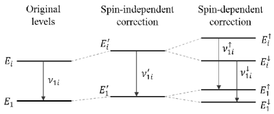
We use nondegenerate perturbation theory for spin-independent interactions and degenerate perturbation theory for spin-dependent interactions. After some calculation, we find the energy shifts are given by
| (61) |
in the laboratory frame, where the square inside the square root denotes summation over , . The upper and lower signs indicate neutrons with spins aligned along and opposite the direction , respectively. This direction typically differs for different energy levels because it depends on the unperturbed eigenenergies . As a result, the spin-up state of the -th energy level is oriented differently from the spin-up state of the -th energy level when . The generic analysis of transitions between different energy levels can therefore be involved.
For present purposes, it suffices to adopt the standard practice tables of taking only one of the coefficients and to be nonzero at a time. In this scenario, the spins of either spin-up or spin-down states with different energy levels are aligned, simplifying the discussion of transitions. Also, when only is nonzero, different energy levels are split by the same amount. This has no effect on the frequencies measured in the experiment, so we can disregard in this context. Therefore, assuming only one of and is nonzero, we find the energy differences in the laboratory frame are shifted according to
| (62) |
The form of the expression (62) is independent of rotations of the observer frame and thus can be applied with the coefficients and in the Sun-centered frame instead. By comparing it to the experimental results cetal18 , we deduce the constraints
| (63) |
at the 95% confidence level. The latter bound is derived using the standard deviation of the transition frequencies. Note that the constraints (63) are sharper than those in Eq. (59) because transition frequencies can be measured more precisely than critical heights. Using the appropriate rows in Table 3, the above constraints can be converted into conditions on linearized coefficients and hence on the terms in the Lagrange density given by Tables 1 and 2. We can also extract constraints on the tilde coefficients introduced in Table 5. These are incorporated in Table 6 as the entries associated with Ref. cetal18 .
In parallel with the result (58) for critical heights, the expression (62) for the transition frequencies contains hidden dependence on the local sidereal time emerging from the rotation (1) to the Sun-centered frame. The signs represent spin projections along a direction determined by coefficients in the laboratory frame, which rotates at the sidereal frequency when expressed in the Sun-centered frame. The measured values of the transition frequencies can therefore fluctuate harmonically with when polarized neutrons are used. This signal would be worthwhile seeking in future experimental analyses.
VII Summary
In this work, we investigate observable effects arising in underlying theories based on non-Riemann geometry or having a nongeometric basis, and we constrain them by analyzing existing results from laboratory experiments and astrophysical observations. The theoretical framework adopted for this purpose is effective field theory based on GR coupled to the SM, allowing for arbitrary backgrounds. We focus on the LLI-EDV class of underlying theories, which permit comparatively straightforward treatment of observable signals, and consider primarily the effects of spin-gravity couplings linearized around Minkowski spacetime. Numerous first constraints are deduced on background coefficients in these beyond-Riemann scenarios.
The methodology adopted for this work is described in Sec. II. The motivation and setup are presented for the class of underlying theories considered here, with all fermion-gravity terms of mass dimension in the linearized Lagrange density displayed in Table 1. The relationships between the linearized coefficients appearing in this table and the underlying coefficients in the full Lagrange density are listed in Table 2. We use a generalized Foldy-Wouthuysen technique to extract the corresponding nonrelativistic hamiltonian , with the explicit form for a uniform gravitational acceleration given in Eqs. (4), (5), (6), (8), (10), and (12). The match between the nonrelativistic coefficients appearing in and the linearized coefficients appearing in is provided in Table 3. We also discuss the dependence of the coefficients on particle and antiparticle flavor.
Using this methodology, we explore the implications for the underlying theories that arise from a variety of laboratory experiments and astrophysical observations. We begin in Sec. III by considering constraints on linearized coefficients that can be inferred from existing measurements performed at different gravitational potentials. The generic dependence of a coefficient on the potential is given in Eq. (20). Many of the experimental results in the literature turn out to be conveniently discussed in terms of a set of tilde coefficients, defined in Table 5. The constraints obtained here apply to the electron, proton, neutron, and muon sectors, and they are summarized in Tables 6 and 7.
In Sec. IV, we turn attention to experiments comparing the gravitational accelerations of different atoms. The modifications to the gravitational acceleration relevant to these studies are given by the operator (29). Constraints from tests with 87Sr atoms of different spins are derived and reported in Eqs. (34) and (35), while those from tests with 87Rb atoms in different hyperfine states are obtained in Eqs. (39) and (40). Future prospects are discussed for measurements of the gravitational acceleration of antimatter, in particular for comparisons using H atoms and antiatoms. Among the results is the derivation of the Eötvös ratio (44) describing the difference in free fall between H and in various hyperfine states.
Studies of the quantum properties of nonrelativistic neutrons also offer interesting sensitivity to fermion-gravity couplings. In Sec. V, we examine interferometric experiments with split coherent neutron beams that traverse different paths in a gravitational potential. Constraints from the classic COW experiment with unpolarized neutrons are derived in Eq. (48), while ones from the spin-dependent OffSpec experiment are obtained in Eq. (52). We also discuss measurements of the quantum bound states of nonrelativistic neutrons above a neutron mirror. Published results on the critical heights for low-lying bound states lead to the constraints (59), while measurements of transition frequencies yield the bounds (63). Where appropriate, all our constraints on nonrelativistic coefficients are translated into ones on tilde coefficients and reported in Table 6.
The methodology and results outlined in this work establish techniques for investigating gravitational effective field theories arising from a class of underlying theories with beyond-Riemann structures. The various calculations presented here illustrate the derivation of experimental and observational constraints for these theories. The work establishes a path for further phenomenological and experimental studies seeking unconventional signals in realistic gravitational effective field theories, with considerable prospects for discovery.
Acknowledgments
This work was supported in part by the U.S. Department of Energy under grant DE-SC0010120 and by the Indiana University Center for Spacetime Symmetries.
References
- (1) See, for example, S. Weinberg, Proc. Sci. CD 09, 001 (2009).
- (2) V.A. Kostelecký, Phys. Rev. D 69, 105009 (2004).
- (3) V.A. Kostelecký and Z. Li, Phys. Rev. D 103, 024059 (2021).
- (4) R. Bluhm, Phys. Rev. D 91, 065034 (2015); Phys. Rev. D 92, 085015 (2015); R. Bluhm and A. Sehic, Phys. Rev. D 94, 104034 (2016); R. Bluhm, H. Bossi, and Y. Wen, Phys. Rev. D 100, 084022 (2019).
- (5) V.A. Kostelecký and M. Mewes, Phys. Rev. D 66, 056005 (2002); Phys. Rev. D 80, 015020 (2009).
- (6) For a review see, for example, G.M. Tino, L. Cacciapuoti, S. Capozziello, G. Lambiase, and F. Sorrentino, Prog. Part. Nucl. Phys. 112, 103772 (2020).
- (7) B. Riemann, Über die Hypothesen welche der Geometrie zu Grunde liegen, in R. Baker, C. Christensen, and H. Orde, Bernhard Riemann, Collected Papers, Kendrick Press, Heber City, Utah, 2004; P. Finsler, Über Kurven und Flächen in allgemeinen Räumen, University of Göttingen dissertation, 1918, Verlag Birkhäuser, Basel, Switzerland, 1951.
- (8) For a textbook discussion of Riemann-Finsler geometry see, for example, D. Bao, S.-S. Chern, and Z. Shen, An Introduction to Riemann-Finsler Geometry, Springer, New York, 2000.
- (9) V.A. Kostelecký, Phys. Lett. B 701, 137 (2011); V.A. Kostelecký, N. Russell, and R. Tso, Phys. Lett. B 716, 470 (2012); B.R. Edwards and V.A. Kostelecký, Phys. Lett. B 786, 319 (2018).
- (10) M.A. Javaloyes and B.L. Soares, Class. Quantum Grav. 38, 025002 (2020); A. Bernal, M.A. Javaloyes and M. Sánchez, Universe 6, 55 (2020); M.A. Javaloyes and M. Sánchez, Rev. Real Acad. Ciencias Exactas, Físicas, y Naturales A 114, 30 (2020).
- (11) A. Triantafyllopoulos, E. Kapsabelis, and P.C. Stavrinos, Eur. Phys. J. Plus 135, 557 (2020); A. Triantafyllopoulos and P.C. Stavrinos, Class. Quant. Grav. 35, 085011 (2018); G. Papagiannopoulos, S. Basilakos, A. Paliathanasis, S. Savvidou, and P.C. Stavrinos, Class. Quant. Grav. 34, 225008 (2017).
- (12) E. Minguzzi, Phys. Rev. D 95, 024019 (2017).
- (13) M.D.C. Torri, S. Bertini, M. Giammarchi, and L. Miramonti, JHEAp 18, 5 (2018); V. Antonelli, L. Miramonti, and M.D.C. Torri, Eur. Phys. J. C 78, 667 (2018).
- (14) C. Lämmerzahl and V. Perlick, Int. J. Geom. Meth. Mod. Phys. 15, 1850166 (2018).
- (15) E. Caponio and A. Masiello, Universe 6, 59 (2020); E. Caponio and G. Stancarone, Class. Quant. Grav. 35, 085007 (2018).
- (16) R.T. Thompson, Phys. Rev. D 97, 065001 (2018).
- (17) X. Li, Phys. Rev. D 98, 084030 (2018).
- (18) J.E.G. Silva, R.V. Maluf and C.A.S. Almeida, Phys. Lett. B 798, 135009 (2019).
- (19) L. Bubuianu and S.I. Vacaru, Eur. Phys. J. Plus 135, 148 (2020).
- (20) J.J. Relancio and S. Liberati, Phys. Rev. D 101, 064062 (2020).
- (21) A. Fuster, S. Heefer, C. Pfeifer and N. Voicu, Universe 6, 64 (2020).
- (22) M. Schreck, Phys. Lett. B 793, 70 (2019); J.A.A.S. Reis and M. Schreck, Phys. Rev. D 97, 065019 (2018); Phys. Rev. D 103, 095029 (2021).
- (23) D. Colladay, Phys. Lett. B 772, 694 (2017).
- (24) J. Foster and R. Lehnert, Phys. Lett. B 746, 164 (2015).
- (25) N. Russell, Phys. Rev. D 91, 045008 (2015).
- (26) See, for example, C.W. Misner, K.S. Thorne, and J.A. Wheeler, Gravitation, W.H. Freeman, San Francisco, 1973; R.M. Wald, General Relativity, University of Chicago Press, Chicago, 1984. For the differential geometry of fiber bundles see, for example, S. Kobayashi and K. Nomizu, Foundations of Differential Geometry, Wiley, New York, 1963.
- (27) V.A. Kostelecký and R. Potting, Phys. Rev. D 51, 3923 (1995).
- (28) V.A. Kostelecký and S. Samuel, Phys. Rev. D 39, 683 (1989); V.A. Kostelecký and R. Potting, Nucl. Phys. B 359, 545 (1991).
- (29) D. Colladay and V.A. Kostelecký, Phys. Rev. D 55, 6760 (1997); Phys. Rev. D 58, 116002 (1998).
- (30) R. Lehnert, W.M. Snow, and H. Yan, Phys. Lett. B 730, 353 (2014); V.A. Kostelecký, N. Russell, and J.D. Tasson, Phys. Rev. Lett. 100, 111102 (2008).
- (31) R. Lehnert, W.M. Snow, Z. Xiao, and R. Xu, Phys. Lett. B 772, 865 (2017); J. Foster, V.A. Kostelecký, and R. Xu, Phys. Rev. D 95, 084033 (2017).
- (32) L.L. Foldy and S.A. Wouthuysen, Phys. Rev. 78, 29 (1950).
- (33) V.A. Kostelecký and C.D. Lane, J. Math. Phys. 40, 6245 (1999).
- (34) V.A. Kostelecký and R. Lehnert, Phys. Rev. D 63, 065008 (2001).
- (35) B. Gonçalves, Y.N. Obukhov and I.L. Shapiro, Phys. Rev. D 80, 125034 (2009); B. Gonçalves, M.M. Dias Júnior, and B.J. Ribeiro, Phys. Rev. D 90, 085026 (2014); Phys. Rev. D 99, 096015 (2019).
- (36) V.A. Kostelecký and J.D. Tasson, Phys. Rev. D 83, 016013 (2011).
- (37) V.A. Kostelecký and M. Mewes, Phys. Rev. D 85, 096005 (2012).
- (38) V.A. Kostelecký and M. Mewes, Phys. Rev. D 88, 096006 (2013).
- (39) Y. Bonder, Phys. Rev. D 88, 105011 (2013).
- (40) C.D. Lane, Phys. Rev. D 94, 025016 (2016).
- (41) Z. Xiao, Phys. Rev. D 98, 035018 (2018).
- (42) L. Parker, Phys. Rev. D 22, 1922 (1980); X. Huang and L. Parker, Phys. Rev. D 79, 024020 (2009).
- (43) C.G. de Oliveira and J. Tiomno, Nuovo Cim. 24, 672 (1962).
- (44) J. Audretsch and G. Schaefer, Gen. Rel. Grav. 9, 489 (1978).
- (45) E. Fischbach, B.S. Freeman and W.K. Cheng, Phys. Rev. D 23, 2157 (1981).
- (46) F.W. Hehl and W.T. Ni, Phys. Rev. D 42, 2045 (1990).
- (47) Y.Q. Cai and G. Papini, Phys. Rev. Lett. 66, 1259 (1991).
- (48) J.C. Huang, Ann. der Phys. 506, 53 (1994).
- (49) K. Varju and L.H. Ryder, Phys. Rev. D 62, 024016 (2000).
- (50) Yu.N. Obukhov, Phys. Rev. Lett. 86, 192 (2001).
- (51) A.J. Silenko and O.V. Teryaev, Phys. Rev. D 71, 064016 (2005).
- (52) J. Leitner and S. Okubo, Phys. Rev. 136,B1542 (1964); N.D. Hari Dass, Phys. Rev. Lett. 36, 393 (1976); A. Peres, Phys. Rev. D 18, 2739 (1978).
- (53) For a review see, for example, W.T. Ni, Rep. Prog. Phys. 73, 056901 (2010).
- (54) V.A. Kostelecký and C.D. Lane, Phys. Rev. D 60, 116010 (1999).
- (55) V.A. Kostelecký and A.J. Vargas, Phys. Rev. D 98, 036003 (2018).
- (56) T. Schmidt, Z. Phys. 106, 358 (1937).
- (57) See, for example, J.M. Blatt and V.F. Weisskopf, Theoretical Nuclear Physics, Wiley, New York, 1952.
- (58) V.A. Kostelecký and N. Russell, Data Tables for Lorentz and CPT Violation, Rev. Mod. Phys. 83, 11 (2011); arXiv:0801.0287v14 (2021).
- (59) J.D. Prestage et al., Phys. Rev. Lett. 54, 2387 (1985).
- (60) T.E. Chupp et al., Phys. Rev. Lett. 63, 1541 (1989).
- (61) C.J. Berglund et al., Phys. Rev. Lett. 75, 1879 (1995).
- (62) L.-S. Hou, W.-T. Ni, and Y.-C.M. Li, Phys. Rev. Lett. 90, 201101 (2003).
- (63) F. Canè et al., Phys. Rev. Lett. 93, 230801 (2004).
- (64) C.D. Lane, Phys. Rev. D 72, 016005 (2005).
- (65) P. Wolf et al., Phys. Rev. Lett. 96, 060801 (2006).
- (66) B. Altschul, Phys. Rev. D 74, 083003 (2006).
- (67) H. Müller et al., Phys. Rev. Lett. 99, 050401 (2007).
- (68) B. Altschul, Astropart. Phys. 28, 380 (2007).
- (69) B. Altschul, Phys. Rev. D 75, 041301(R) (2007).
- (70) B. Altschul, Phys. Rev. D 78, 085018 (2008).
- (71) B.R. Heckel et al., Phys. Rev. D 78, 092006 (2008).
- (72) J.M. Brown et al., Phys. Rev. Lett. 105, 151604 (2010); in V.A. Kostelecký, ed., CPT and Lorentz Symmetry V, World Scientific, Singapore, 2011.
- (73) M.A. Hohensee et al., Phys. Rev. Lett. 106, 151102 (2011).
- (74) M. Smiciklas et al., Phys. Rev. Lett. 107, 171604 (2011).
- (75) S.K. Peck et al., Phys. Rev. A 86, 012109 (2012).
- (76) A. Fittante and N. Russell, J. Phys. G 39, 125004 (2012).
- (77) K. Tullney et al., Phys. Rev. Lett. 111, 100801 (2013).
- (78) F. Allmendinger et al., Phys. Rev. Lett. 112, 110801 (2014); in V.A. Kostelecký, ed., CPT and Lorentz Symmetry VI, World Scientific, Singapore, 2014.
- (79) B.M. Roberts et al., Phys. Rev. Lett. 113, 081601 (2014).
- (80) B.M. Roberts et al., Phys. Rev. D 90, 096005 (2014).
- (81) B. Botermann et al., Phys. Rev. Lett. 113, 120405 (2014); Phys. Rev. Lett. 114, 239902 (2015).
- (82) Y.V. Stadnik and V.V. Flambaum, Eur. Phys. J. C 75, 110 (2015).
- (83) A. Lo et al., Phys. Rev. X 6, 011018 (2016).
- (84) V.V. Flambaum, Phys. Rev. Lett. 117, 072501 (2016); V.V. Flambaum and M.V. Romalis, Phys. Rev. Lett. 118, 142501 (2017).
- (85) C. Smorra et al., Nature 550, 371 (2017).
- (86) N. Flowers, C. Goodge, and J.D. Tasson, Phys. Rev. Lett. 119, 201101 (2017).
- (87) H. Pihan-Le Bars et al., Phys. Rev. D 95, 075026 (2017).
- (88) C. Sanner et al., Nature 567, 204 (2019).
- (89) B. Altschul, Symmetry 13, 688 (2021).
- (90) J. Bailey et al., Nucl. Phys. 150, 1 (1979).
- (91) R. Bluhm, V.A. Kostelecký, and C.D. Lane, Phys. Rev. Lett. 84, 1098 (2000).
- (92) V.W. Hughes et al., Phys. Rev. Lett. 87, 111804 (2001)
- (93) M. Deile et al., Muon 2 Collaboration, in V.A. Kostelecký, ed., CPT and Lorentz Symmetry II, World Scientific, Singapore, 2002.
- (94) G.W. Bennett et al., Muon 2 Collaboration, Phys. Rev. Lett. 100, 091602 (2008).
- (95) J.P. Noordmans, C.J.G. Onderwater, H.W. Wilschut, and R.G.E. Timmermans, Phys. Rev. D 93, 116001 (2016).
- (96) S. Aghababaei, M. Haghighat, and I. Motie, Phys. Rev. D 96, 115028 (2017).
- (97) See, for example, D. Turcotte and G. Schubert, Geodynamics, third edition, Cambridge University Press, Cambridge, 2014. For gravity-field models based on satellite observations see, for example, A. Bezděk, J. Sebera, J. Klokoňik, and J. Kostelecký, Adv. Space Res. 53, 412 (2014).
- (98) A.H. Gomes, V.A. Kostelecký, and A.J. Vargas, Phys. Rev. D 90, 076009 (2014).
- (99) V.A. Kostelecký and A.J. Vargas, Phys. Rev. D 92, 056002 (2015).
- (100) V.A. Kostelecký and Y. Ding, Phys. Rev. D 94, 056008 (2016).
- (101) V.A. Kostelecký and Z. Li, Phys. Rev. D 99, 056016 (2019).
- (102) M.G. Tarallo, T. Mazzoni, N. Poli, D.V. Sutyrin, X. Zhang, and G.M. Tino, Phys. Rev. Lett. 113, 023005 (2014).
- (103) X.C. Duan et al., Phys. Rev. Lett. 117, 023001 (2016).
- (104) G. Cronenberg et al., Nat. Phys. 14, 1022 (2018).
- (105) S. Afach et al., Phys. Dark Univ. 22, 162 (2018).
- (106) C. Qin and C. Shao, Phys. Lett. B 820, 136471 (2021).
- (107) R. Bluhm, V.A. Kostelecký, C.D. Lane, and N. Russell, Phys. Rev. Lett. 88, 090801 (2002); Phys. Rev. D 68, 125008 (2003).
- (108) B. Abi et al., Phys. Rev. Lett. 126, 141801 (2021).
- (109) B.J. Venema, P.K. Majumder, S.K. Lamoreaux, B.R. Heckel,and E.N. Fortson, Phys. Rev. Lett. 68, 135 (1992).
- (110) A.N. Youdin, D. Krause, K. Jagannathan, L.R. Hunter, and S.K. Lamoreaux, Phys. Rev. Lett. 77, 2170 (1996).
- (111) D.F. Jackson Kimball, J. Dudley, Y. Li, D. Patel, and J. Valdez, Phys. Rev. D 96, 075004 (2017).
- (112) B. Heckel, E.G. Adelberger, C.E. Cramer, T.S. Cook, S. Schlamminger, and U. Schmidt, Phys. Rev. D 78, 092006 (2008).
- (113) A. Kellerbauer et al., Nucl. Instr. Meth. Phys. Res. B 266, 351 (2008); S. Aghion et al., Nature Commun. 5, 4538 (2014); J. Storey et al., Hyperfine Int. 228, 151 (2014).
- (114) C. Amole et al., Nat. Commun. 4, 1785 (2013); P. Hamilton, A. Zhmoginov, F. Robicheaux, J. Fajans, J.S. Wurtele, and H. Müller, Phys. Rev. Lett. 112, 121102 (2014).
- (115) P. Indelicato et al., Hyperfine Int. 228, 141 (2014); P. Perez and Y. Sacquin, Class. Quantum Grav. 29, 184008 (2012); G. Chardin et al., CERN report CERN-SPSC-2011-029, September 30, 2011.
- (116) For a review see, for example, M. Charlton, S. Eriksson, and G.M. Shore, Antihydrogen and Fundamental Physics, Springer, Cham, Switzerland, 2020.
- (117) E.P. Wigner, Z. Phys. 43, 624 (1927); C. Eckart, Rev. Mod. Phys. 2, 305 (1930).
- (118) J.M. Morton et al., Nucl. Phys. A 161, 228 (1971).
- (119) L.R. Medsker et al., Phys. Rev. C 12, 1516 (1975).
- (120) R. Eötvös, V. Pekár, and E. Fekete, Ann. Phys. (Berlin) 373, 11 (1922).
- (121) P. Asenbaum, C. Overstreet, M. Kim, J. Curti and M.A. Kasevich, Phys. Rev. Lett. 125, 191101 (2020).
- (122) K. Zhang, M.K. Zhou, Y. Cheng, L.L. Chen, Q. Luo, W.J. Xu, L.S. Cao, X.C. Duan, and Z.K. Hu, Chin. Phys. Lett. 37, 043701 (2020).
- (123) G. Lüders, Det. Kong. Danske Videnskabernes Selskab Mat.-fysiske Meddelelser 28, no. 5 (1954); J.S. Bell, Birmingham University Ph.D. thesis (1954); Proc. Roy. Soc. (London) A 231 (1955) 479; W. Pauli, p. 30 in W. Pauli, ed., Niels Bohr and the Development of Physics, McGraw-Hill, New York, 1955.
- (124) R. Colella, A.W. Overhauser, and S.A. Werner, Phys. Rev. Lett. 34, 1472 (1975).
- (125) J.L. Staudenmann et al., Phys. Rev. A 21, 1419 (1980).
- (126) S.A. Werner, H. Kaiser, M. Arif, and R. Clothier, Physica BC 151, 22 (1988).
- (127) K.C. Littrell et al., Phys. Rev. A 56, 1767 (1997).
- (128) G. van der Zouw, M. Weber, J. Felber, R. Gahler, P. Geltenbort, and A. Zeilinger, Nucl. Instrum. Methods Phys. Res. A440, 568 (2000).
- (129) V.-O. de Haan, J. Plomp, A.A. van Well, M.T. Rekveldt, Y.H. Hasegawa, R.M. Dalgliesh, and N.-J. Steinke, Phys. Rev. A 89, 063611 (2014).
- (130) For a review see, for example, H. Abele and H. Leeb, New J. Phys. 14, 055010 (2012).
- (131) V.V. Nesvizhevsky et al., Nature 415, 297 (2002); Phys. Rev. D 67, 102002 (2003); Eur. Phys. J. C 40, 479 (2005).
- (132) A. Martín-Ruiz and C.A. Escobar, Phys. Rev. D 97, 095039 (2018); C.A. Escobar and A. Martín-Ruiz, Phys. Rev. D 99, 075032 (2019).
- (133) A.N. Ivanov, M. Wellenzohn, and H. Abele, Phys. Lett. B 797, 134819 (2019).
- (134) Z. Xiao and L. Shao, J. Phys. G 47, 085002 (2020).