On Simple Mechanisms for Dependent Items

Abstract

We study the problem of selling $n$ heterogeneous items to a single buyer, whose values for different items are dependent. Under arbitrary dependence, Hart and Nisan [30] show that no simple mechanism can achieve a non-negligible fraction of the optimal revenue even with only two items. We consider the setting where the buyer’s type is drawn from a correlated distribution that can be captured by a Markov Random Field, one of the most prominent frameworks for modeling high-dimensional distributions with structure.

If the buyer’s valuation is additive or unit-demand, we extend the result to all MRFs and show that $\max\{\textsc{SRev},\textsc{BRev}\}$ can achieve an $\Omega\left(\frac{1}{e^{O(\Delta)}}\right)$-fraction of the optimal revenue, where $\Delta$ is a parameter of the MRF that is determined by how much the value of an item can be influenced by the values of the other items. We further show that the exponential dependence on $\Delta$ is unavoidable for our approach and a polynomial dependence on $\Delta$ is unavoidable for any approach. When the buyer has a XOS valuation, we show that $\max\{\textsc{SRev},\textsc{BRev}\}$ achieves at least an $\Omega\left(\frac{1}{e^{O(\Delta)}+\frac{1}{\sqrt{n\gamma}}}\right)$-fraction of the optimal revenue, where $\gamma$ is the spectral gap of the Glauber dynamics of the MRF. Note that in the special case of independently distributed items, $\Delta=0$ and $\frac{1}{n\gamma}\leq 1$, and our results recover the known constant factor approximations for a XOS buyer [41]. We further extend our parametric approximation to several other well-studied dependency measures such as the Dobrushin coefficient [27] and the inverse temperature. In particular, we show that if the MRF is in the high temperature regime, $\max\{\textsc{SRev},\textsc{BRev}\}$ is still a constant factor approximation to the optimal revenue even for a XOS buyer. Our results are based on the Duality-Framework by Cai et al. [14] and a new concentration inequality for XOS functions over dependent random variables.

1 Introduction

The design of revenue-optimal auctions for selling multiple items is a central problem in Economics and Computer Science. In the past decade, significant progress has been made, first in efficient computation of revenue-optimal auctions [18, 19, 1, 10, 2, 11, 12, 15, 13, 3, 6, 24], and then in the identification of simple auctions that achieve constant factor approximations to the optimal revenue [4, 45, 41, 14, 21, 17] under the item-independence assumptions.  Despite being theoretically appealing, item-independence is an unrealistic assumption in practice. In this paper, we go beyond the item-independence assumption and study simple and approximately optimal auctions for selling dependent items.

Unfortunately, strong negative results exist if we allow the items to be arbitrarily dependent [8, 30]. For example, Hart and Nisan [30] show that the revenue of the best deterministic mechanism is unboundedly smaller than the revenue of the optimal randomized mechanism even when we are only selling two correlated items to a single buyer. Since all simple mechanisms in the literature are deterministic, the result also implies that no simple mechanism that has been considered so far can provide any guarantee to the revenue for even two correlated items. Arguably, however, high-dimensional distributions that arise in practice are rarely arbitrary, as arbitrary high-dimensional distributions cannot be represented efficiently, and are known to require exponentially many samples to learn or even perform the most basic statistical tests on them; see e.g. [25] for a discussion. To overcome the curse of dimensionality, a major focus of Statistics and Machine Learning has been on identifying and exploiting the structural properties of high-dimensional distributions for succinct representation, efficient learning, and efficient statistical inference. There are several widely-studied frameworks to model the structure of dependence in high-dimensional distributions. In this work, we propose capturing the dependence between item values using one of the most prominent graphical models – Markov Random Fields (MRFs). Note that MRFs are fully general and can be used to express arbitrary high-dimensional distributions. The main advantage of MRFs is that there are several natural complexity parameters that allow the user to tune the dependence structure in the distributions represented by MRFs from product measures all the way up to arbitrary distributions. Our goal is to provide parametric approximation ratios of simple mechanisms that degrade gracefully with respect to these natural parameters.

MRFs are formally defined in Definition 2. Intuitively, a MRF can be thought of as a graph (or a hypergraph) where each node represents a random variable (or item value in our case). There is a potential function associated with each edge that captures the correlation between the two incident random variables. How does it represent a joint distribution? The probability for a particular realization or the random variables, or known as a configuration of the random field, is proportional to the exponential of the total potential of the configuration. MRF is a flexible model. For example, we can capture the degree of (positive or negative) correlations between two random variables by controlling the corresponding potential function. Here we provide a stylistic example to illustrate the suitability of MRFs for modeling buyers’ joint value distributions. Imagine that we manage a car dealership. A potential buyer is hoping to purchase one car, i.e., has a unit-demand valuation. The dealership carries various brands and types of vehicles, and will like to find the optimal way to price each car. However, it would be naïve to assume the buyer’s value for each car is independently distributed. The example in Figure 1 demonstrates how a MRF can better capture the customer’s joint value distribution for different cars.

Figure 1: We draw a green edge (or a red edge) between two cars if their values are positively correlated (or negative correlated). The car in the center is an electric coupe with a retro design. Its value is positively correlated with the two electric cars on its left and the two small coupes on its right, but is negatively correlated with the pick-up truck.

1.1 Main Results and Techniques

We focus on the single buyer case and allow the buyer’s valuation to be as general as a XOS function (a.k.a. a fractionally subadditive function).  We consider the two most extensively studied forms of simple mechanisms: selling the items separately and selling the grand bundle. We use SRev and BRev to denote the optimal revenue obtainable by these two types of mechanisms respectively. In a sequence of papers, it was shown that $\max\{\textsc{SRev},\textsc{BRev}\}$ is a constant factor approximation to the optimal revenue for a single additive or unit-demand buyer under the item-independence assumption [18, 4, 14].  Our first main result extends the above approximation to any MRFs. The approximation ratio degrades with the maximum weighted degree $\Delta$ that captures the degree of dependence among the item values.

Parameter I: Maximum Weighted Degree $\Delta$.

The formal definition can be found in Definition 4. As we mentioned, a MRF can be thought of as a graph (or a hypergraph) where each node represents a random variable. The weight of an edge is related to the maximum absolute value the corresponding potential function can take and represents the “strength” of the dependence between two incident random variables. The weighted degree of a random variable is simply the sum of weights from all incident edges. If the maximum weighted degree $\Delta$ of a MRF is small, then no random variable can depend strongly on many other random variables. Note that $\Delta=0$ when the random variables are independent, and the instance constructed by Hart and Nisan [30] corresponds to a MRF with $\Delta=\infty$.

1. For a single additive or unit-demand buyer whose type is generated by a MRF with maximum weighted degree $\Delta$, $\max\{\textsc{SRev},\textsc{BRev}\}=\Omega\left(\frac{\textsc{OPT}}{\exp(O(\Delta))}\right)$, where OPT is the optimal revenue.

The formal statement of the result is in Theorem 1 and 2. We further show that the dependence on $\Delta$ is necessary. For any sufficiently large number $C$, there exists a MRF with $\Delta=O(C)$ such that $\max\{\textsc{SRev},\textsc{BRev}\}$ is no more than $\frac{\textsc{OPT}}{C^{1/7}}$ (Theorem 3) using a modification of the Hart-Nisan construction [30]. Although there is still an exponential gap between our upper and lower bounds, it shows that whenever Result I fails to provide a constant factor approximation (independent of the number of items), no constant factor approximation is possible without further restrictions on the dependency. We leave it as an open question to close the gap between our upper and lower bounds. The main tool we use is a generalization of the prophet inequality to the case where the rewards are sampled from a MRF (Lemma 3). The overall analysis is similar to the one used by Cai et al. [14] for the item-independent case. We show that the exponential dependence on $\Delta$ is unavoidable for this type of analysis in Theorem 8. More specifically, a key step of the analysis involves approximating the optimal revenue in a single-dimensional setting, known as the copies setting, using SRev. Theorem 8 constructs an instance such that the optimal revenue in the copies setting is at least $\exp(\Delta)$ times larger than $\max\{\textsc{SRev},\textsc{BRev}\}$.

Rubinstein and Weinberg [41] show that, under the item-independence assumption, $\max\{\textsc{SRev},\textsc{BRev}\}$ is still a constant factor approximation to the optimal revenue for a buyer whose valuation is a subadditive function. Our second main result extends their result to any MRFs when the buyer’s valuation is a XOS function. The approximation ratio depends on $\Delta$ and the spectral gap of the Glauber Dynamics $\gamma$.

Parameter II: Spectral Gap of the Glauber Dynamics $\gamma$.

A common way to generate a sample from a high-dimensional distribution is via a Markov Chain Monte Carlo method known as the Glauber dynamics (see Definition 5). The spectral gap $\gamma$ of the Glauber dynamics is the difference between the largest eigenvalue $\lambda_{1}=1$ and the second largest eigenvalue $\lambda_{2}$ of the transition matrix of the Glauber dynamics. It is well-known that $\lambda_{2}$ is strictly less than $1$ for any MRFs [36], so $\gamma$ is always strictly positive.

1. For a single XOS buyer whose type is generated by a MRF, $\max\{\textsc{SRev},\textsc{BRev}\}=\Omega\left(\frac{\textsc{OPT}}{\exp({O(\Delta)})+\frac{1}{\sqrt{n\gamma}}}\right)$, where $n$ is the number of items, $\gamma$ is the spectral gap of the Glauber Dynamics, and $\Delta$ is the maximum weighted degree. 

Some remarks are in order. First, our approximation ratio holds for any MRFs. Second, for any $n$-dimensional random vector $X=(x_{1},\ldots,x_{n})$, the $X_{i}$’s are considered weakly dependent if the spectral gap $\gamma=\Omega(\frac{1}{n})$. For example, when the $x_{i}$’s are independent, $\gamma\geq\frac{1}{n}$. Finally, the condition $\gamma\geq\Omega(\frac{1}{n})$ is extensively studied in probability theory. The condition is satisfied under the Dobrushin uniqueness condition (see Section 6 for details), a well-known sufficient condition that ensures weak dependency; it implies rapid mixing of the Glauber dynamics (i.e., they mix in time $O(n\log n)$); it also guarantees that polynomial functions concentrate in Ising models [29, 26].

The formal statement of Result II can be found in Theorem 4. The analysis follows the same general framework by Cai and Zhao [17]. The major new challenge is to prove that any XOS function $g(X)$ concentrates, when $X$ is a drawn from a high-dimensional distribution $D$. Proving concentration inequalities for non-linear functions over dependent random variables is a non-trivial task that lies at the heart of many high-dimensional statistical problems. We prove a parametric concentration inequality for XOS functions that depends on the spectral gap of the Glauber dynamics for $D$ (Lemma 13). The proof is based on a combination of the Poincaré inequality and a special property of XOS functions – the self-boundingness. We believe this concentration inequality may be of independent interest. An interesting question is whether the approximation ratio needs to depend on both $\Delta$ and $\gamma$. We show that the dependence on $\Delta$ is crucial, as no approximation can be obtained with only restriction on the spectral gap even for a single additive or unit-demand buyer (Theorem 7).  We do not know whether it is possible to obtain an approximation that only depends on $\Delta$ for a XOS buyer and leave it as an open question.  We suspect such an improvement requires proving a parametric concentration inequality for XOS functions that only depend on the maximum weighted degree $\Delta$, which we believe will have further applications.

Our Results under Other Weak Dependence Conditions.

There are several alternative ways to parametrize the degree of dependency in a high-dimensional distribution. We focus on two prominent ones – the Dobrushin coefficient and the inverse temperature of a MRF, and discuss how our approximation results change under these conditions. We first consider the Dobrushin coefficient and its relaxations. An important concept is the influence matrix.

Influence Matrix and the Dobrushin Condition

For any $n$-dimensional random vector $\mathbf{X}=(X_{1},\ldots,X_{n})$, we define the influence of variable $j$ on variable $i$ as

$$\alpha_{i,j}:=\sup_{\begin{subarray}{c}x_{-i-j}\\ x_{j}\neq x^{\prime}_{j}\end{subarray}}d_{TV}\left(F_{X_{i}\mid X_{j}=x_{j},X_{-i-j}=x_{-i-j}},F_{X_{i}\mid X_{j}=x^{\prime}_{j},X_{-i-j}=x_{-i-j}}\right),~{}$$

where $F_{X_{i}\mid X_{-i}=x_{-i}}$ denotes the conditional distribution of $X_{i}$ given $X_{-i}=x_{-i}$. Let $\alpha_{i,i}:=0$ for each $i$. We define the influence matrix $A:=\left(\alpha_{i,j}\right)_{i,j\in[n]}$. When the $X_{i}$’s are weakly dependent, the entries of $A$ should have small values. The Dobrushin Coefficient, defined as $||A||_{\infty}=\max_{i\in[n]}\sum_{j\in[n]}\alpha_{i,j}$, was originally introduced by Dobrushin [27] in the study of Gibbs measures. The Dobrushin coefficient less than $1$ is known as the Dobrushin uniqueness condition, under which the Gibbs distribution has a unique equilibrium, hence the name. The condition can be viewed as a sufficient condition that guarantees weak dependence and has been extensively studied in statistical physics and probability literature (see e.g. [28, 43]). As the spectral radius of any matrix is no more than its $L_{\infty}$ norm, a relaxation of the Dobrushin uniqueness condition is to restrict the spectral radius $\rho$ of $A$ to be less than $1$. We show that $n\gamma\geq 1-\rho$ (Lemma 16), so we can replace the dependence on $n\gamma$ with $1-\rho$ in Result II when the item values are weakly dependent (Theorem 5). We also show that the dependence on $\Delta$ is necessary. Without any restriction on $\Delta$, the gap between $\max\{\textsc{SRev},\textsc{BRev}\}$ and the optimal revenue could be unbounded even under the Dobrushin uniqueness condition for an additive or unit-demand buyer (Theorem 7). Next, we consider how the approximation guarantee degrades in terms of the inverse temperature of a MRF.

Inverse Temperature $\beta$ of a MRF

The inverse temperature is related to both the maximum weighted degree and the Dobrushin coefficient. See Definition 3 for the formal definition. Intuitively, as the inverse temperature increases (or temperature drops), the dependence between the different random variables strengthens. When the inverse temperature is $0$, the MRF represents a product distribution. The high temperature regime is when the inverse temperature is less than $1$. This parameter often controls when phase transitions in the behavior of MRFs happen, and hence the name. The Dobrushin coefficient always upper bounds the inverse temperature. Recently, MRFs in the high temperature regime have been applied to model weakly dependent random variables [22].

We show that if the MRF is in the high temperature regime, then its maximum weighted degree $\Delta<1$ and the spectral gap $\gamma$ of the Glauber dynamics has value at least $\frac{1-\beta}{n}$. As a corollary of Result II, we have

1. For a single XOS buyer, $\max\{\textsc{SRev},\textsc{BRev}\}=\Omega\left(\sqrt{1-\beta}\cdot\textsc{OPT}\right)$, where $\beta<1$ is the inverse temperature.

The result states that as long as the inverse temperature is bounded away from $1$ by any constant, $\max\{\textsc{SRev},\textsc{BRev}\}$ achieves a constant fraction of the optimal revenue. Theorem 6 contains the formal statement of the result.

We summarize our results in Table 1 and the relationship between the parameters in Figure 2.

Maximum Weighted Degree $\Delta$ Maximum Weighted Degree $\Delta$ and Spectral Gap $\gamma$ Spectral Gap $\gamma$ or Dobrushin Coefficient $\alpha<1$ Inverse Temperature $\beta<1$ Additive or Unit-Demand UB: $\Omega\left(\frac{\textsc{OPT}}{\exp(O(\Delta))}\right)$ (Theorem 2 and 1) LB: $O\left(\frac{\textsc{OPT}}{\Delta^{1/7}}\right)$ (Theorem 3) UB: $\Omega\left(\frac{\textsc{OPT}}{\exp(O(\Delta))}\right)$ ($\leftarrow$) LB: $O\left(\frac{\textsc{OPT}}{\Delta^{1/7}}\right)$ ($\leftarrow$) Unbounded (Theorem 7) UB: $\Omega\left(\sqrt{1-\beta}\cdot\textsc{OPT}\right)$ ($\downarrow$) LB: open XOS UB: open LB: $O\left(\frac{\textsc{OPT}}{\Delta^{1/7}}\right)$ ($\uparrow$) UB: $\Omega\left(\frac{\textsc{OPT}}{\exp({O(\Delta)})+\frac{1}{\sqrt{n\gamma}}}\right)$ (Theorem 4) LB: $O\left(\frac{\textsc{OPT}}{\Delta^{1/7}}\right)$ ($\leftarrow$) Unbounded ($\uparrow$) UB: $\Omega\left(\sqrt{1-\beta}\cdot\textsc{OPT}\right)$ (Theorem 6) LB: open

Table 1: The table contains our upper bounds and lower bounds of the approximation ratio of $\max\{\textsc{SRev},\textsc{BRev}\}$ in various settings. The results are listed based on (i) the valuation of the buyer and (ii) the parameters the approximation ratio can depend on. In our table, an arrow means the result follows from the result that the arrow points to.

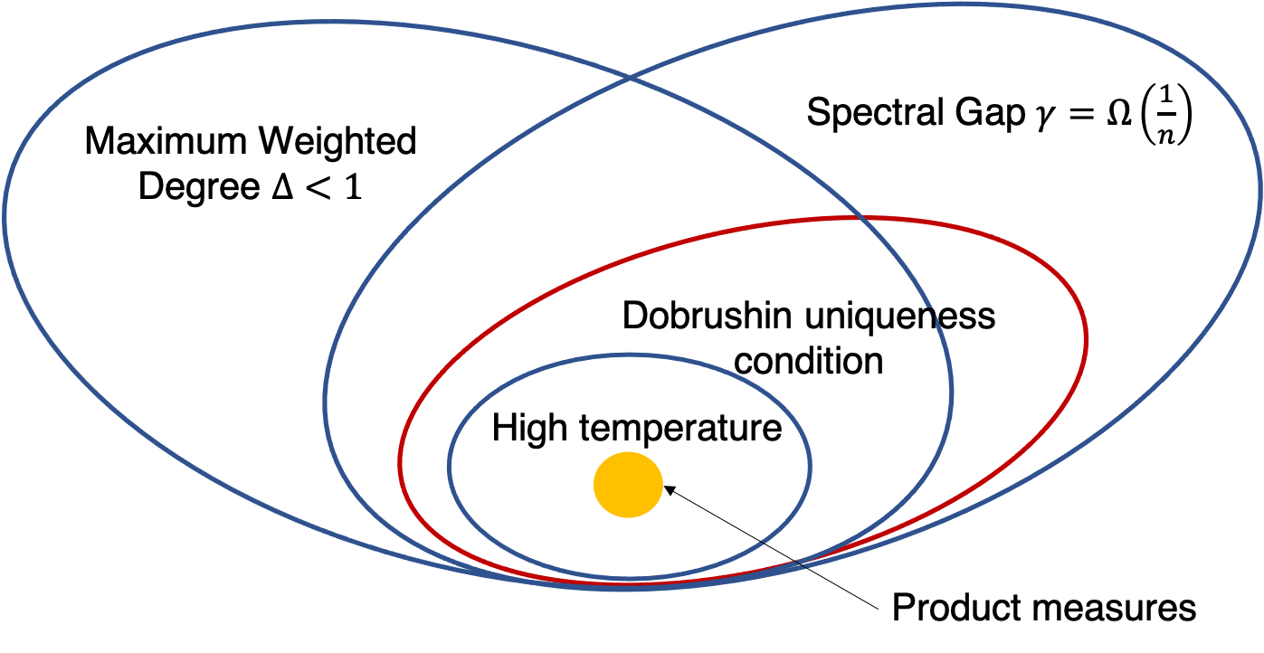
Figure 2: The relationship between the parameters: inverse temperature, Dobrushin coefficient, maximum weighted degree, and spectral gap of the Glauber dynamics.

1.2 Related Work

Simple vs. Optimal Auctions

There has been a large body of work on multi-item auction design focusing on either approximation results under item-independence  [18, 19, 1, 15, 37, 4, 45, 41, 14, 21, 17] or impossibility to approximate under arbitrary dependence [8, 30]. Two types of models have been studied for items with limited dependence. The first model considers a specific type of dependence where each item’s value is a linear combination of “independent features” [20, 5]. Unlike MRFs, this model cannot express arbitrary structure of dependence. Indeed, the values of any two items can only be positively correlated under this model. The second model considers the smoothed complexity of the problem [38]. Their result applies to arbitrary dependence structure between the item values, but only achieves an approximation ratio that is exponential in the number of items. Our paper is the first to consider a model general enough to capture arbitrary structure of dependence and obtain parametric approximation ratios that are independent of the number of items.

MRFs and Weakly Dependent Random Variables

There has been growing interest in understanding the behavior of weakly dependent random variables that can be captured by a MRF in the high temperature regime or under the Dobrushin uniqueness condition [29, 26, 22]. In mechanism design, Brustle et al. [9] is the first to propose modeling dependent item values using MRFs in multi-item auctions, but they focus on the sample complexity of learning nearly optimal auctions.

2 Preliminaries

Basic Notation

We consider an auction where a seller is selling $n$ heterogeneous items to a single buyer. We denote the buyer’s type $\bm{t}$ as $\langle t_{i}\rangle_{i=1}^{n}$, where $t_{i}$ is the buyer’s private information about item $i$. We use $D$ to denote the distribution of $\bm{t}$, $D_{i}$ to denote the marginal distribution of $t_{i}$, and $D_{i\mid c_{-i}}$ to denote the distribution of $t_{i}$ conditioned on $t_{-i}=c_{-i}$. We use $\textsc{Supp}(\mathcal{F})$ to denote the support of distribution $\mathcal{F}$, and $T_{i}=\textsc{Supp}(D_{i})$ and $T=\textsc{Supp}(D)$. Moreover, we use $f(c)$ to denote $\Pr_{\bm{t}\sim D}[\bm{t}=c]$. For any item $i$ and any $c_{i}\in T_{i}$ and $c_{-i}\in T_{-i}$, we use $f_{i}(c_{i})$ to denote $\Pr_{t_{i}\sim D_{i}}[t_{i}=c_{i}]$, $f_{i}(c_{i}\mid c_{-i})$ to denote $\Pr_{\bm{t}\sim D}[t=(c_{i},c_{-i})]\over\Pr_{\bm{t}\sim D}[t_{-i}=c_{-i}]$, $f_{-i}(c_{-i})$ to denote $\Pr_{\bm{t}\sim D}[t_{-i}=c_{-i}]$, and $f_{-i}(c_{-i}\mid c_{i})$ to denote $\Pr_{\bm{t}\sim D}[t=(c_{i},c_{-i})]\over\Pr_{\bm{t}\sim D}[t_{i}=c_{i}]$. We also define $F_{i}(c_{i})=\Pr_{{t}_{i}\sim D_{i}}\left[{t}_{i}\leq c_{i}\right]$ and $F_{i}(c_{i}\mid c_{-i})=\Pr_{{t}_{i}\sim D_{i\mid c_{-i}}}\left[{t}_{i}\leq c_{i}\right]$. Finally, when the buyer’s type is $\bm{t}$, her valuation for a set of items $S$ is denoted by $v(\bm{t},S)$.

We investigate the performance of simple mechanisms for several well-studied valuation classes.

Definition 1 (Valuation Classes).

We define several classes of valuations formally.

• Constrained Additive: interpret $t_{i}$ as the value of item $i$, and $v(\bm{t},S)=\max_{R\subseteq S,R\in\mathcal{I}}\sum_{i\in R}t_{i}$, where $\mathcal{I}\subseteq 2^{[m]}$ is a downward closed set system over the items specifying the feasible bundles. When $\mathcal{I}=2^{[m]}$, the valuation is called Additive. When $\mathcal{I}$ contains all the singletons and the empty set, the valuation is called unit-demand.

• XOS/Fractionally Subadditive: interpret $t_{i}$ as $\{t_{i}^{(k)}\}_{k\in[K]}$ that encodes all the possible values associated with item $i$, and $v(t,S)=\max_{k\in[K]}\sum_{i\in S}t_{i}^{(k)}$.

It is well known that the class of XOS valuations contains all constrained additive valuations.

Mechanism

A mechanism $M$ is specified by an allocation rule and a payment rule. We use $\pi$ to denote the allocation rule, and $\pi_{i}(\bm{t})$ is the probability that the buyer receives item $i$ when she reports type $\bm{t}$. We also use $p(\bm{t})$ to denote the buyer’s payment when she reports type $\bm{t}$. We assume the buyer has quasi-linear utility. We say a mechanism $M$ is Incentive Compatible (IC) if the buyer cannot increase their expected utility by misreporting their type, and Individual Rational (IR) if the buyer has non-negative expected utility when they report their type truthfully to the mechanism.

Given $D$, valuation function $v(\cdot,\cdot)$, we use $\textsc{Rev}(M,v,D)$ to denote the expected revenue of an IC and IR mechanism $M$. We slightly abuse notation to use $\textsc{Rev}(D)$ to denote the optimal revenue achievable by any IC and IR mechanism under distribution $D$.

Throughout the paper, we use the following notations for the simple mechanisms we consider.

- $\textsc{SRev}(v,D)$ denotes the optimal expected revenue achievable by any posted price mechanism, and we use SRev for short if there is no ambiguity. - $\textsc{BRev}(v,D)$ denotes the optimal expected revenue achievable by selling a grand bundle and we use BRev for short if there is no ambiguity.

2.1 Markov Random Fields

Definition 2 (Markov Random Fields).

A Markov Random Field (MRF) is defined by a hypergraph $G=(V,E)$. Associated with every vertex $v\in V$ is a random variable $X_{v}$ taking values in some alphabet $\Sigma_{v}$, as well as a potential function $\psi_{v}:\Sigma_{v}\rightarrow\mathbb{R}$. Associated with every hyperedge $e\subseteq V$ is a potential function $\psi_{e}:\Sigma_{e}\rightarrow\mathbb{R}$. In terms of these potentials, we define a probability distribution $\pi$ associating to each vector $\bm{c}\in\bigtimes_{v\in V}\Sigma_{v}$ probability $\pi(\bm{c})$ satisfying: $\pi(\bm{c})\propto\prod_{v\in V}e^{\psi_{v}(c_{v})}\prod_{e\in E}e^{\psi_{e}(\bm{c}_{e})}$,where $\Sigma_{e}$ denotes $\times_{v\in e}\Sigma_{v}$ and $\bm{c}_{e}$ denotes $\{c_{v}\}_{v\in e}$.

We refer the interested readers to [35, 32] and the references therein for more details about MRFs. Throughout the paper, when we say the type distribution $D$ is a MRF over a hypergraph $G=(V,E)$, if $V=[n]$, $t_{i}=x_{i}$, $T_{i}=\Sigma_{i}$, and there exists a collection of potential functions $\{\psi_{i}(\cdot)\}_{i\in[n]}$ and $\{\psi_{e}(\cdot)\}_{e\in E}$ so that the corresponding distribution $p(\cdot)$ equals to $D$. If there are only pairwise potentials, then $G$ is a graph. We say that a random variable $\bm{t}$ is generated by a MRF, if $\bm{t}$ is sampled from a distribution that is represented by the MRF.

Next, we define two ways to measure the degree of dependence in a MRF.

Definition 3.

Let random variable $\bm{t}$ be generated by a Markov Random Field over a hypergraph $G=([n],E)$, we define the Markov influence between item $i$ and $j$ to be: $\beta_{i,j}(\bm{t}):=\max_{\bm{x}\in\times_{\ell\in[n]}T_{\ell}}{\left|\sum_{\begin{subarray}{c}e\in E:\\ i,j\in e\end{subarray}}\psi_{e}(\bm{x}_{e})\right|}$. We further define the inverse temperature of the MRF as $\beta(\bm{t}):=\max_{i\in[n]}\sum_{j\neq i}\beta_{i,j}(\bm{t})$. We say random variable/type $\bm{t}$ is in the high temperature regime if $\beta(\bm{t})<1$.

Definition 4.

Given a random variable/type $\bm{t}$ generated by a Markov Random Field over a hypergraph $G=([n],E)$, we define the weighted degree of item $i$ as: $d_{i}(\bm{t}):=\max_{\bm{x}\in\times_{i\in[n]}T_{i}}\left|\sum_{e\in E:i\in e}{\psi_{e}(\bm{x}_{e})}\right|$, and the maximum weighted degree as $\Delta(\bm{t}):=\max_{i\in[n]}d_{i}(\bm{t})$.

Remark 1.

Both $\beta(\bm{t})$ and $\Delta(\bm{t})$ capture the degree of dependence between the items. Note that $\Delta(\bm{t})\leq\beta(\bm{t})$ for any MRF $\bm{t}$, and it is possible that $\beta(\bm{t})=\Omega(d\cdot\Delta(\bm{t}))$, where $d$ is the size of the largest hyperedge in $G$. When $\bm{t}$ is drawn from a product measure, both $\beta(\bm{t})$ and $\Delta(\bm{t})$ are $0$. In general, restricting $\beta(\bm{t})$ and $\Delta(\bm{t})$ to be small ensures that the item values are only weakly dependent.

To achieve our results, we need another important concept – the Glauber dynamics. In Section 5, we relate the approximation ratio achievable by simple mechanisms to the spectral gap of the Glauber dynamics of the MRF.

Definition 5 (Glauber Dynamics).

Let $X_{1},\ldots,X_{n}$ be an $n$-dimensional random vector drawn from distribution $\pi$. Let $\Omega$ be the support of $\pi$. The Glauber dynamics for $\pi$ is a reversible Markov chain with state space $\Omega$. The Glauber chain moves from state $x\in\Omega$ as follows: an index $i$ is chosen uniformly at random from $[n]$, and a new state $y$ is chosen so that (i) $y_{j}=x_{j}$ for all $j\neq i$; (ii) draw $y_{i}$ from the conditional distribution $\pi\mid X_{-i}=x_{-i}$. It is not hard to verify that the Glauber dynamics is a reversible Markov chain with stationary distribution $\pi$.

Remark 2.

When $\pi$ is the distribution that can be represented by a MRF $G=(V,E)$, the Glauber dynamics has state space $\bigtimes_{v\in V}\Sigma_{v}$. The Glauber chain moves from state $x\in\bigtimes_{v\in V}\Sigma_{v}$ as follows: a vertex $v$ is chosen uniformly at random from $V$, and a new state $y$ is chosen so that (i) $y_{u}=x_{u}$ for all $u\neq v$; (ii) for any $c\in\Sigma_{v}$, $y_{v}=c$ w.p. $\frac{\exp(\psi_{v}(c))\Pi_{e:v\in e}\exp(\psi_{e}\left(c,x_{e/\{v\}}\right))}{\sum_{c^{\prime}\in\Sigma_{v}}\exp(\psi_{v}(c^{\prime}))\Pi_{e:v\in e}\exp(\psi_{e}\left(c^{\prime},x_{e/\{v\}}\right))}$, in other words, sample $y_{v}$ according to the distribution conditioned on $y_{-v}=x_{-v}$. Note that for a MRF, the Glauber dynamics is an irreiducible Markov chain, so $\pi$ is its only stationary distribution. The Glauber dyanamics is a standard method for generating samples from a MRF, as it does not require computing the partition function, which is often a computationally intractable task.

3 Markov Random Fields: Basic Properties and Tools

We first present some basic properties of a MRF. Roughly speaking, we show that the conditional distribution can be approximated by the corresponding marginal distribution of $D$, and the approximation quality only depends $\Delta(\bm{t})$.

Lemma 1.

Let random variable $\bm{t}$ be generated by a MRF. Then for any $t_{i}\in T_{i},t_{-i}\in T_{-i}$:

$$\frac{\exp(\psi_{i}(t_{i}))}{\sum_{t^{\prime}_{i}\in T_{i}}\exp(\psi_{i}(t_{i}^{\prime}))}\exp(-2\Delta(\bm{t}))\leq f_{i}(t_{i}\mid t_{-i})\leq\frac{\exp(\psi_{i}(t_{i}))}{\sum_{t^{\prime}_{i}\in T_{i}}\exp(\psi_{i}(t_{i}^{\prime}))}\exp(2\Delta(\bm{t}))$$

and

$$f_{i}(t_{i})\cdot\exp(-4\Delta(\bm{t}))\leq f_{i}(t_{i}\mid t_{-i})\leq f_{i}(t_{i})\cdot\exp(4\Delta(\bm{t})).$$

Proof.

Note that for any $t_{i}^{\prime}\in T_{i}$, ${f\left((t_{i},t_{-i})\right)\over f\left((t_{i}^{\prime},t_{-i})\right)}={\exp(\psi_{i}(t_{i}))\over\exp(\psi_{i}(t^{\prime}_{i}))}\cdot{\exp\left(\sum_{e\in E,i\in e}\psi_{e}\left(t_{i},t_{-i}\right)_{e}\right)\over\exp\left(\sum_{e\in E,i\in e}\psi_{e}\left(t^{\prime}_{i},t_{-i}\right)_{e}\right)}$.

Clearly,

$${\exp(\psi_{i}(t_{i}))\over\exp(\psi_{i}(t^{\prime}_{i}))}\cdot\exp(-2\Delta(\bm{t}))\leq{f\left((t_{i},t_{-i})\right)\over f\left((t_{i}^{\prime},t_{-i})\right)}\leq{\exp(\psi_{i}(t_{i}))\over\exp(\psi_{i}(t^{\prime}_{i}))}\cdot\exp(2\Delta(\bm{t})).$$

Since $f_{i}(t_{i}\mid t_{-i})={f\left((t_{i},t_{-i})\right)\over\sum_{t_{i}^{\prime}\in T_{i}}f\left((t_{i}^{\prime},t_{-i})\right)}$,

$$\frac{\exp(\psi_{i}(t_{i}))\cdot\exp(-2\Delta(\bm{t}))}{\sum_{t^{\prime}_{i}\in T_{i}}\exp(\psi_{i}(t_{i}^{\prime}))}\leq f_{i}(t_{i}\mid t_{-i})\leq\frac{\exp(\psi_{i}(t_{i}))\exp(2\Delta(\bm{t}))}{\sum_{t^{\prime}_{i}\in T_{i}}\exp(\psi_{i}(t_{i}^{\prime}))}.$$

By Law of Total Probability,

$$f_{i}(t_{i})= \sum_{t_{-i}\in T_{-i}}f_{i}(t_{i}\mid t_{-i})f_{-i}(t_{-i})\in\left[\frac{\exp(\psi_{i}(t_{i}))\cdot\exp(-2\Delta(\bm{t}))}{\sum_{t_{i}^{\prime}\in T_{i}}\exp(\psi_{i}(t_{i}^{\prime}))},\frac{\exp(\psi_{i}(t_{i}))\cdot\exp(2\Delta(\bm{t}))}{\sum_{t_{i}^{\prime}\in T_{i}}\exp(\psi_{i}(t_{i}^{\prime}))}\right].$$

∎

Lemma 2.

Let random variable $\bm{t}$ be generated by a MRF. For any $i$ and any set ${\mathcal{E}}\subseteq T_{i}$ and set ${\mathcal{E}}^{\prime}\subseteq T_{-i}$:

$$\exp(-4\Delta(\bm{t}))\leq{\Pr_{\bm{t}\sim D}\left[t_{i}\in{\mathcal{E}}\land t_{-i}\in{\mathcal{E}}^{\prime}\right]\over\Pr_{t_{i}\sim D_{i}}[t_{i}\in{\mathcal{E}}]\Pr_{t_{-i}\sim D_{-i}}\left[t_{-i}\in{\mathcal{E}}^{\prime}\right]}\leq\exp(4\Delta(\bm{t})).$$

Proof.

Note that $\Pr_{\bm{t}\sim D}\left[t_{i}\in{\mathcal{E}}\land t_{-i}\in{\mathcal{E}}^{\prime}\right]=\sum_{\bm{t}\in{\mathcal{E}}\times{\mathcal{E}}^{\prime}}f_{i}(t_{i}\mid t_{-i})\cdot f_{-i}(t_{-i})$ and $\Pr[t_{i}\in{\mathcal{E}}]\Pr\left[t_{-i}\in{\mathcal{E}}^{\prime}\right]=\sum_{\bm{t}\in{\mathcal{E}}\times{\mathcal{E}}^{\prime}}f_{i}(t_{i})\cdot f_{-i}(t_{-i})$. Hence

$${\Pr_{\bm{t}\sim D}\left[t_{i}\in{\mathcal{E}}\land t_{-i}\in{\mathcal{E}}^{\prime}\right]\over\Pr_{t_{i}\sim D_{i}}[t_{i}\in{\mathcal{E}}]\Pr_{t_{-i}\sim D_{-i}}\left[t_{-i}\in{\mathcal{E}}^{\prime}\right]}=\frac{\sum_{\bm{t}\in{\mathcal{E}}\times{\mathcal{E}}^{\prime}}f_{i}(t_{i}\mid t_{-i})\cdot f_{-i}(t_{-i})}{\sum_{\bm{t}\in{\mathcal{E}}\times{\mathcal{E}}^{\prime}}f_{i}(t_{i})\cdot f_{-i}(t_{-i})}$$

Using Lemma 1 we get that:

$$\frac{\sum_{\bm{t}\in{\mathcal{E}}\times{\mathcal{E}}^{\prime}}f_{i}(t_{i}\mid t_{-i})\cdot f_{-i}(t_{-i})}{\sum_{\bm{t}\in{\mathcal{E}}\times{\mathcal{E}}^{\prime}}f_{i}(t_{i})\cdot f_{-i}(t_{-i})}\leq\exp(4\Delta)\frac{\sum_{\bm{t}\in{\mathcal{E}}\times{\mathcal{E}}^{\prime}}f_{i}(t_{i})\cdot f_{-i}(t_{-i})}{\sum_{\bm{t}\in{\mathcal{E}}\times{\mathcal{E}}^{\prime}}f_{i}(t_{i})\cdot f_{-i}(t_{-i})}=\exp(4\Delta)$$

and

$$\frac{\sum_{\bm{t}\in{\mathcal{E}}\times{\mathcal{E}}^{\prime}}f_{i}(t_{i}\mid t_{-i})\cdot f_{-i}(t_{-i})}{\sum_{\bm{t}\in{\mathcal{E}}\times{\mathcal{E}}^{\prime}}f_{i}(t_{i})\cdot f_{-i}(t_{-i})}\geq\exp(-4\Delta)\frac{\sum_{\bm{t}\in{\mathcal{E}}\times{\mathcal{E}}^{\prime}}f_{i}(t_{i})\cdot f_{-i}(t_{-i})}{\sum_{\bm{t}\in{\mathcal{E}}\times{\mathcal{E}}^{\prime}}f_{i}(t_{i})\cdot f_{-i}(t_{-i})}=\exp(-4\Delta).$$

∎

Prophet Inequality for MRF

Equipped with Lemma 2, we provide a generalization of the Prophet inequality when the rewards in different stages are dependent and generated by a MRF. We can think of the prophet inequality problem, as finding a good policy for a gambler in a multi-round game. At the $i$-th round, the gambler is given the choice to accept a reward or to continue to the next round. The goal of the gambler is to find a policy that obtains high expected reward, given the distributions of the rewards at each round. Prophet inequalities have been obtained when the rewards between stages are independent [34, 42, 33] or can be expressed a a linear combination of some independent random variables [31].

Lemma 3.

Let $\bm{t}=(t_{1},\ldots,t_{n})$ be an $n$-dimensional random vector generated by a MRF. There are totally $n$ rounds, and the reward of round $i$ is $g_{i}(t_{i})$, where $g_{i}$ is an arbitrary function. The total reward of the prophet is $\operatorname{\mathbb{E}}_{\bm{t}}\left[\max_{i\in[n]}g_{i}(t_{i})\right]$. We denote by $\textsc{Reward}_{\bm{t}}\left[\{g_{i}\}_{i\in[n]},\tau\right]$ the expected of reward of the following policy – accept any reward that is at least $\tau$. The following inequality holds if we choose $\tau^{*}=\textsc{Median}_{\bm{t}}\left(\max_{i\in[n]}g_{i}(t_{i})\right)$ (i.e., $\Pr[\max_{i\in[n]}g_{i}(t_{i})\geq\tau^{*}]=1/2$),

$$\frac{\exp(-4\Delta(\bm{t}))}{2}\operatorname{\mathbb{E}}_{\bm{t}}\left[\max_{i\in[n]}g_{i}(t_{i})\right]\leq\textsc{Reward}_{\bm{t}}\left[\{g_{i}\}_{i\in[n]},\tau^{*}\right].$$

Proof.

The proof is similar to the case when all $t_{i}$ are independent.

It is not hard to see that

$$\operatorname{\mathbb{E}}_{\bm{t}}\left[\max_{i\in[n]}g_{i}(t_{i})\right]\leq\tau^{*}+\sum_{i\in[n]}\operatorname{\mathbb{E}}_{t_{i}\sim D_{i}}\left[\left(g_{i}(t_{i})-\tau^{*}\right)^{+}\right].$$

We provide a lower bound on $\textsc{Reward}_{\bm{t}}\left[\{g_{i}\}_{i\in[n]},\tau^{*}\right]$.

$$\textsc{Reward}_{\bm{t}}\left[\{g_{i}\}_{i\in[n]},\tau^{*}\right]\geq\Pr_{\bm{t}}\left[\max_{i\in[n]}g_{i}(t_{i})\geq\tau^{*}\right]\cdot\tau^{*}+\sum_{i\in[n]}\operatorname{\mathbb{E}}_{\bm{t}}\left[(g_{i}(t_{i})-\tau^{*})^{+}\cdot\mathds{1}[\max_{j\neq i}g_{j}(t_{j})\leq\tau^{*}]\right]$$

For every $i\in[n]$, we define the set ${\mathcal{E}}_{i}$ as $\{t_{i}\in T_{i}:g_{i}(t_{i})>\tau^{*}\}$ and ${\mathcal{E}}^{\prime}_{i}$ as $\{t_{-i}\in T_{-i}:\max_{j\neq i}g_{j}(t_{j})\leq\tau^{*}\}$. Note that

$$\operatorname{\mathbb{E}}_{\bm{t}}\left[(g_{i}(t_{i})-\tau^{*})^{+}\cdot\mathds{1}[\max_{j\neq i}g_{j}(t_{j})<\tau^{*}]\right] =\sum_{\bm{t}\in{\mathcal{E}}_{i}\times{\mathcal{E}}_{i}^{\prime}}\left(g_{i}(t_{i})-\tau^{*}\right)\cdot f(\bm{t})$$

$$\geq\exp(-4\Delta(\bm{t}))\sum_{\bm{t}\in{\mathcal{E}}_{i}\times{\mathcal{E}}_{i}^{\prime}}\left(g_{i}(t_{i})-\tau^{*}\right)\cdot f_{i}(t_{i})f_{-i}(t_{-i})$$

$$=\exp(-4\Delta(\bm{t}))\operatorname{\mathbb{E}}_{t_{i}\sim D_{i}}\left[\left(g_{i}(t_{i})-\tau^{*}\right)^{+}\right]\Pr_{t_{-i}\sim D_{-i}}[t_{-i}\in{\mathcal{E}}^{\prime}_{i}]$$

The inequality is due to Lemma 2. Putting everything together, we know that

$$\textsc{Reward}_{\bm{t}}\left[\{g_{i}\}_{i\in[n]},\tau^{*}\right]\geq{1\over 2}\cdot\tau^{*}+\sum_{i\in[n]}\operatorname{\mathbb{E}}_{t_{i}\sim D_{i}}\left[(g_{i}(t_{i})-\tau^{*})^{+}\right]\cdot{\exp(-4\Delta(\bm{t}))\over 2},$$

which is at least ${\exp(-4\Delta(\bm{t}))\over 2}$ of the upper bound we provide for $\operatorname{\mathbb{E}}_{\bm{t}}\left[\max_{i\in[n]}g_{i}(t_{i})\right]$. ∎

4 Simple Mechanisms for a Unit-Demand or Additive Buyer under MRF

In this section, we first use the duality framework from [14, 17] to construct an upper bound of $\textsc{Rev}(D)$. Next, we prove that if the buyer has either unit-demand or additive valuation across the items, $\max\{\textsc{SRev},\textsc{BRev}\}$ is a $O(\exp(12\Delta(\bm{t})))$-approximation or a $O(\exp(4\Delta(\bm{t})))$-approximation of $\textsc{Rev}(D)$, respectively.

4.1 Benchmark of the Optimal Revenue for Constrained Additive Valuations

In this section, we use the duality framework from [14, 17] to construct an upper bound of $\textsc{Rev}(D)$. We describe a benchmark of the optimal revenue for all constrained additive valuations. Deriving a benchmark for XOS valuations requires some extra care, and we provide details of the derivation in Section 5.1 when we study XOS valuations. We first remind the readers the partition of type space used in [14, 17].

Definition 6 (Partition of the Type Space for Constrained Additive Valuations [14, 17]).

We partition the type space $T$ into $n$ regions, where $R_{i}=\{\bm{t}\in T:i~{}\text{is the smallest index in}~{}\operatorname{argmax}_{i^{\prime}\in[n]}t_{i^{\prime}}\}$. If $\bm{t}\in R_{i}$, we call item $i$ the favorite item of type $\bm{t}$.

To handle the dependence across the items, we introduce some new notations to specify the benchmark.

Definition 7 (Ironed Virtual Value).

Let $D$ be the type distribution. For any $\bm{t}\in R_{i}$, we use $\phi_{i}(t_{i})$ to denote the ironed Myerson’s virtual value for distribution $D_{i}$, $\phi_{i}(t_{i}\mid t_{-i})$ to denote the ironed Myerson’s virtual value when we ironed $D_{i\mid t_{-i}}$ over interval $[\max_{j\neq i}t_{j},\max\textsc{Supp}(D_{i\mid t_{-i}})]$.

If $D_{i\mid t_{-i}}$ is a regular distribution and $t^{\prime}_{i}=\operatorname{argmin}\{\hat{t}\in\textsc{Supp}(D_{{i}\mid t_{-i}}):\hat{t}>t_{i}\}$,

$$\phi_{i}(t_{i}\mid t_{-i})=t_{i}-\frac{\left(t_{i}^{\prime}-t_{i}\right)\cdot\Pr_{\hat{\bm{t}}\sim D}\left[\hat{t}_{i}>t_{i}\land\hat{t}_{-i}=t_{-i}\right]}{f(\bm{t})}=t_{i}-\frac{\left(t_{i}^{\prime}-t_{i}\right)\cdot\left(1-F_{i}(t_{i}\mid t_{-i})\right)}{f_{i}(t_{i}\mid t_{-i})}.$$

Moreover, $\phi_{i}(t_{i}\mid t_{-i})$ always satisfies the following property:

$$\max_{p\geq\max_{j\neq i}t_{j}}p\cdot(1-F_{i}(p\mid t_{-i}))=\sum_{\begin{subarray}{c}t_{i}:~{}(t_{i},t_{-i})\in R_{i}\end{subarray}}f_{i}(t_{i}\mid t_{-i})\cdot\phi_{i}(t_{i}\mid t_{-i})^{+},$$

where $x^{+}=\max\{x,0\}$.

Lemma 4 contains the benchmark we use. See Appendix A for more details about Lemma 4.

Lemma 4 (Benchmark of Optimal Revenue for Constrained Additive Valuations).

Given a distribution $D$ over the type space $T$, and a mechanism $M=(\pi,p)$, if the buyer’s valuation $v$ is constrained additive, then we have the following benchmark:

$$\textsc{Rev}(M,v,D)\leq \sum_{\bm{t}\in T}\sum_{i\in[n]}f(\bm{t})\cdot\pi_{i}(\bm{t})\cdot\phi_{i}(t_{i}\mid t_{-i})\cdot\mathds{1}\left[\bm{t}\in R_{i}\right]\quad(\textsc{Single})$$

$$\qquad\qquad+\sum_{\bm{t}\in T}\sum_{i\in[n]}f(\bm{t})\cdot\pi_{i}(\bm{t})\cdot t_{i}\cdot\mathds{1}\left[\bm{t}\notin R_{i}\right](\textsc{Non-Favorite})$$

$$\leq \sum_{\bm{t}\in T}\sum_{i\in[n]}f(\bm{t})\cdot\pi_{i}(\bm{t})\cdot\phi_{i}(t_{i}\mid t_{-i})\cdot\mathds{1}\left[\bm{t}\in R_{i}\right]\quad(\textsc{Single})$$

$$\qquad\qquad+\sum_{i\in[n]}\sum_{t_{i}>r}f_{i}(t_{i})\cdot t_{i}\cdot\Pr_{\bm{t}^{\prime}\sim D}\left[\bm{t}^{\prime}\notin R_{i}\mid t^{\prime}_{i}=t_{i}\right]\quad(\textsc{Tail})$$

$$\qquad\qquad\qquad\qquad+\sum_{i\in[n]}\sum_{t_{i}\leq r}f_{i}(t_{i})\cdot t_{i}\quad(\textsc{Core}),$$

where $r=\textsc{SRev}(v,D)$.

Single-Dimensional Copies Setting:

In the analysis of unit-demand bidders with independent items [19, 14], the optimal revenue is upper bounded by the optimal revenue in the single-dimensional copies setting defined in [19]. We make use of the same technique in our analysis. There is a single item for sale, and we construct $n$ agents, where agent $i$ has value $t_{i}$ for winning the item. Notice that this is a single-dimensional setting, as each agent’s type is specified by a single number.

4.2 A Unit-Demand Buyer

In this section, we show that a simple posted price mechanism can extract $O(\exp(12\Delta(\bm{t})))$ fraction of the optimal revenue when the type distribution $D$ is a MRF. We first use the revenue of the Ronen’s lookahead auction [40] to upper bound the benchmark from Lemma 4.  Ronen’s auction first identifies the highest bidder, and offers a take it or leave it price to the highest bidder to maximize the revenue conditioned on the other bidders’ types. The proof follows from the definition of Ronen’s lookahead auction and basic properties of MRF presented in Lemma 1 and 2. We postpone the proof to Appendix B.

Lemma 5.

Let the type distribution $D$ be represented by a MRF, $M$ be any IC and IR mechanism for a unit-demand buyer, and $\textsc{Ronen}^{\textsc{Copies}}$ be revenue of the Ronen’s lookahead auction [40] in the Copies settings with respect to $D$. The following inequalities hold:

$$\max\{\textsc{Single},\textsc{Non-Favorite}\} \leq\textsc{Ronen}^{\textsc{Copies}}$$

$$\textsc{Ronen}^{\textsc{Copies}} \leq\exp(8\Delta(\bm{t}))\operatorname{\mathbb{E}}_{\bm{t}}\left[\max_{i\in[n]}\phi_{i}(t_{i})^{+}\right].$$

Equipped with Lemma 5, we can apply the prophet inequality for MRF to show that a posted-price mechanism can obtain expected revenue that is at least $\Omega\left(\frac{\textsc{Ronen}^{\textsc{Copies}}}{\exp(12\Delta(\bm{t}))}\right)$. We delay the proof to Appendix B.

Theorem 1.

Let the type distribution $D$ be represented by a MRF. If the buyer’s valuation is unit-demand, then there exists a posted-price mechanism $M$ with prices $\{p_{i}\}_{i\in[n]}$ that obtains expected revenue at least $\textsc{Rev}(D)\over 8\exp(12\Delta(\bm{t}))$.

Is it possible to improve the dependence on $\Delta$? In Theorem 8, we show that if we use the optimal revenue in the COPIES setting as a benchmark of the optimal revenue in the original setting, then the exponential dependence on $\Delta(\bm{t})$ is unavoidable.

4.3 An Additive Buyer

In this section, we show that $\max\{\textsc{SRev},\textsc{BRev}\}$ is a $O(\exp(4\Delta(\bm{t})))$ approximation of the optimal revenue when the type distribution $D$ is a MRF. We denote by $r_{i}$ the revenue of Myerson’s auction for selling item $i$ only. We use $r=\sum_{i\in[n]}r_{i}$ to denote SRev, as the revenue collected from item $i$ only depends on the marginal distribution $D_{i}$. We first upper bound the terms Single and Tail by $\exp(4\Delta(t))\cdot\textsc{SRev}$. The proof follows from a combination of the standard analysis of the terms Single and Tail from [14, 17] with properties of MRFs (Lemma 2). We postpone the proof to Appendix C.

Lemma 6.

Let the type distribution $D$ be a MRF and $M$ be any IC and IR mechanism for an additive buyer. The following inequalities holds: $\textsc{Single}\leq\exp(4\Delta(\bm{t}))\cdot\textsc{SRev}$ and $\textsc{Tail}\leq\exp(4\Delta(\bm{t}))\cdot\textsc{SRev}$.

Finally, we analyze the Core. We define new random variables $C_{i}=t_{i}\cdot\mathds{1}[t_{i}\leq r]$. Let $C=\sum_{i=1}^{n}C_{i}$. Note that $\operatorname{\mathbb{E}}[C]=\textsc{Core}$. We first provide an upper bound on $\textsc{Var}[C]$, and show that if we sell the grand bundle at an appropriate price, its revenue is close to the Core. Note that under the item-independence assumption, it is not hard to show that $\textsc{Var}[C]$ is upper bounded by $2r^{2}$ [4, 14]. However, this analysis does not extend to the case where the buyer type is generated by a MRF. We first obtain a new upper bound of $\textsc{Var}[C]$. As $C=\sum_{i=1}^{n}C_{i}$, we have $\textsc{Var}[C]=\sum_{i\in[n]}\textsc{Var}[C_{i}]+\sum_{i\neq j}\textsc{Cov}[C_{i},C_{j}]$. We further bound $\sum_{i\in[n]}\textsc{Var}[C_{i}]$ by $2r^{2}$ using the standard analysis in [4, 14] and each covariance $\textsc{Cov}[C_{i},C_{j}]$ using properties of MRF (Lemma 2). The proof is postponed to Appendix C.

Lemma 7.

Let the type distribution $D$ be represented by a MRF. For any $i,j\in[n]$, $\textsc{Cov}[C_{i},C_{j}]\leq(\exp(4\Delta(\bm{t}))-1)\operatorname{\mathbb{E}}[C_{i}]\operatorname{\mathbb{E}}[C_{j}]$. Moreover, $\textsc{Var}[C]\leq 2r^{2}+(\exp(4\Delta(\bm{t}))-1)\operatorname{\mathbb{E}}[C]^{2}$.

In the item-independence case, the standard analysis [4, 14] applies Chebyshev’s inequality to show that the seller can sell the grand bundle at price $\operatorname{\mathbb{E}}[C]-2r$ with probability at least $1/2$, which implies that Core is $O(\textsc{BRev}+\textsc{SRev})$. As our upper bound on $\textsc{Var}[C]$ is a lot larger, Chebyshev’s inequality only gives a vacuous bound on the sell probability.  To show that selling the grand bundling is a good approximation of the Core, we set the price of the grand bundle differently and use the Paley-Zygmund inequality to prove that either the sell probability is high or the Core is within a constant factor of $r$. The proof of Theorem 2 can be found in Appendix C.

Theorem 2.

Let the type distribution $D$ be represented by a MRF. If the buyer’s valuation is additive, then

$$\left(2\exp(4\Delta(\bm{t}))+\sqrt{2}\right)\cdot\textsc{SRev}+8\left(\exp(4\Delta(t))+1\right)\cdot\textsc{BRev}\geq\textsc{Rev}(D).$$

In the following theorem, we show that the approximation ratio must have polynomial dependence on $\Delta(\bm{t})$. Our proof is based on a modification of the hard instance by Hart and Nisan [30]. They construct a joint distribution over two items with support size $m$ and show that the optimal revenue is at least $m^{1/7}\cdot\max\{\textsc{BRev},\textsc{SRev}\}$. Unfortunately, their construction requires $\Delta$ to be infinite. We show how to modify their construction so that the new distribution has maximum weighted degree $\Delta=O(m)$, and the gap between the optimal revenue and $\max\{\textsc{BRev},\textsc{SRev}\}$ remains to be $m^{1/7}$. The key is to show that under the new distribution, no type shows up too rarely, and the optimal revenue, SRev, and BRev remain roughly the same. The proof is postponed to Appendix F.

Theorem 3.

For any sufficiently large $m\in\mathbb{N}$, there exists a type distribution over two items represented by a MRF $D$ such that (i) the maximum weighted degree $\Delta$ is at most $C\cdot m$, where $C$ is an absolute constant; (ii) for an additive buyer whose type is sampled from $D$, there exists an absolute constant $C^{\prime}>0$ such that $\textsc{Rev}(D)\geq C^{\prime}m^{1/7}\cdot{\max\{\textsc{BRev}(D),\textsc{SRev}(D)\}}$.

5 Simple Mechanisms for a XOS Buyer

5.1 Duality Framework for XOS Valuations

The benchmark is obtained using essentially the same approach as in [17]. Suppose the buyer has a XOS valuation function $v(\bm{t},S)$. We denote by $V_{i}(\bm{t})=v(\bm{t},\{i\})$. We abuse this notation and we also define for $t_{i}\in T_{i}$, $V_{i}(t_{i})=v((\mathbf{0},\ldots,t_{i},\ldots,\mathbf{0}),\{i\})$, where $\mathbf{0}$ is the all $0$ vector. We summarize the benchmark for a XOS buyer in the following Lemma. More details can be found in Appendix E.

Lemma 8.

Partition the type space $T$ into $n$ regions, where

$$R_{i}:=\{\bm{t}\in T:\text{$f(\bm{t})>0$ and $i$ is the smallest index that belongs in $\operatorname{argmax}_{i\in[n]}V_{i}(\bm{t})$ }\}$$

Let $r=\textsc{SRev}$ be the revenue of the optimal posted price mechanism that allows the buyer to purchase at most one item. Let $C(\bm{t}):=\{i:V_{i}(\bm{t})<2r\}$. For any IC and IR Mechanism $M$, we can bound its revenue by:

$$\textsc{Rev}(M,v,D)\leq 2\sum_{\bm{t}\in T}f(\bm{t})\sum_{i\in[n]}\pi_{i}(\bm{t})\phi(V_{i}(t_{i})\mid\bm{t}_{-i})\mathds{1}[t\in R_{i}]\quad(\textsc{Single})$$

$$\qquad\qquad+4\sum_{i\in[n]}\sum_{\begin{subarray}{c}t_{i}\in T_{i}\\ {V_{i}(t_{i})}\geq 2r\end{subarray}}f(t_{i})\cdot V_{i}(t_{i})\Pr_{\bm{t}^{\prime}\sim D}\left[\bm{t}^{\prime}\notin R_{i}\mid t_{i}^{\prime}=t_{i}\right](\textsc{Tail})$$

$$\qquad\qquad\qquad\qquad+4\sum_{\bm{t}\in T}f(\bm{t})v(\bm{t},C(\bm{t}))\quad(\textsc{Core})$$

5.2 Approximating the Benchmark of a XOS Buyer

In this section, we show how to approximate the optimal revenue of a buyer with a XOS valuation. We first upper bound the term Single  and Tail . The analysis of both terms follows from the combination of the analysis in [17] and Lemma 2.

Lemma 9.

Let the type distribution $D$ be represented by a MRF. If $M$ is an IC and IR mechanism for a buyer with a XOS valuation, then the following inequalities hold

$$\textsc{Single}\leq 4\exp(12\Delta(\bm{t}))\cdot\textsc{SRev}$$

and

$$\textsc{Tail}\leq\exp(8\Delta(\bm{t}))\cdot\textsc{SRev},$$

where SRev is the revenue of the optimal posted price auction, in which the buyer is allowed to purchase at most one item.

5.2.1 Bounding the Core using the Poincaré Inequality

In this section, we show how to bound the Core for a XOS buyer. The Core is the expectation of the random variable $v(\bm{t},C(\bm{t}))$. To show that bundling can achieve a good approximation of the Core, we need to upper bound the variance of $v(\bm{t},C(\bm{t}))$. This is the main task of this section. As $v(\bm{t},\cdot)$ is not additive across the items, our method for the additive valuation (see Lemma 7) no longer applies. We provide a new approach that is based on the Poincaré Inequality and the self-boundingness of XOS functions. We first state the Poincaré Inequality.

Lemma 10 (The Poincaré Inequality (adapted from Lemma 13.12 of [36])).

Let $P$ be a reversible transition matrix on state space $\Omega$ with stationary distribution $\pi$. For any function $g:\Omega\rightarrow\mathbb{R}$, let

$$\mathcal{E}(g):=\frac{1}{2}\sum_{x,y\in\Omega}[g(x)-g(y)]^{2}\pi(x)P(x,y).$$

If $\textsc{Var}_{x\sim\pi}[g(x)]>0$, then

$$\frac{\mathcal{E}(g)}{\textsc{Var}_{x\sim\pi}[g(x)]}\geq\gamma,$$

where $\gamma$ is the spectral gap of $P$.  Moreover, there exists a function $g^{*}:\Omega\rightarrow\mathbb{R}$, such that

$$\frac{\mathcal{E}(g^{*})}{\textsc{Var}_{x\sim\pi}[g^{*}(x)]}=\gamma.$$

Next, we apply Lemma 10 to the Glauber dynamics of the MRF that generates the buyer’s type.

Lemma 11.

Let $D$ be the joint distribution of random variables $\bm{t}=(t_{1},\ldots,t_{n})$ and $P$ be the transition matrix of the Glauber dynamics for $D$. For any function $g:T\rightarrow\mathbb{R}$, we have

$$n\gamma\cdot\textsc{Var}_{\bm{t}\sim D}[g(\bm{t})]\leq\sum_{i\in[n]}\operatorname{\mathbb{E}}_{\bm{t}\sim D}\left[\left(g(t_{i},\bm{t}_{-i})-\operatorname{\mathbb{E}}_{t^{\prime}_{i}\sim D_{i\mid\bm{t}_{-i}}}[g(t^{\prime}_{i},\bm{t}_{-i})]\right)^{2}\right],$$

where $\gamma$ is the spectral gap of $P$. Moreover, there exists a function $g^{*}:T\rightarrow\mathbb{R}$, such that the inequality is tight.

Remark 3.

Lemma 11 is a generalization of the well-known Efron-Stein inequality to dependent random variables. Indeed, when $D$ is a product measure, $\gamma$ is at least $1/n$ and we recover the Efron-Stein inequality. As we demonstrate in Section 6, $\gamma$ is at least $\Omega(1/n)$ under many well-studied conditions of weak dependence, such as the Dobrushin uniqueness condition.

Proof of Lemma 11: According to the definition of the Glauber dynamics, $P$ is a reversible transition matrix on state space $T$ with stationary distribution $D$. Lemma 10 states that

$$\gamma\cdot\textsc{Var}_{\bm{t}\sim D}[g(x)]\leq\frac{1}{2}\sum_{\bm{t},\bm{t}^{\prime}\in T}[g(\bm{t})-g(\bm{t}^{\prime})]^{2}\cdot f(\bm{t})\cdot P(\bm{t},\bm{t}^{\prime}).$$ (1)

By the definition of the Glauber dynamics, the RHS of Inequality (1) is equivalent to

$$\frac{1}{2}\operatorname{\mathbb{E}}_{\bm{t}\sim D}\left[\frac{1}{n}\sum_{i\in[n]}\operatorname{\mathbb{E}}_{t^{\prime}_{i}\sim D_{i\mid\bm{t}_{-i}}}\left[g(\bm{t})-g(t^{\prime}_{i},\bm{t}_{-i})\right]^{2}\right]$$

$$= \frac{1}{n}\sum_{i\in[n]}\operatorname{\mathbb{E}}_{\bm{t}_{-i}\sim D_{-i}}\left[\operatorname{\mathbb{E}}_{t_{i},t^{\prime}_{i}\sim D_{i\mid\bm{t}_{-i}}}\left[\frac{1}{2}\left(g(t_{i},\bm{t}_{-i})-g(t^{\prime}_{i},\bm{t}_{-i})\right)^{2}\right]\right]$$

$$= \frac{1}{n}\sum_{i\in[n]}\operatorname{\mathbb{E}}_{\bm{t}_{-i}\sim D_{-i}}\left[\operatorname{\mathbb{E}}_{t_{i}\sim D_{i\mid\bm{t}_{-i}}}\left[\left(g(t_{i},\bm{t}_{-i})-\operatorname{\mathbb{E}}_{t^{\prime}_{i}\sim D_{i\mid\bm{t}_{-i}}}[g(t^{\prime}_{i},\bm{t}_{-i})]\right)^{2}\right]\right]$$

$$= \frac{1}{n}\sum_{i\in[n]}\operatorname{\mathbb{E}}_{\bm{t}\sim D}\left[\left(g(t_{i},\bm{t}_{-i})-\operatorname{\mathbb{E}}_{t^{\prime}_{i}\sim D_{i\mid\bm{t}_{-i}}}[g(t^{\prime}_{i},\bm{t}_{-i})]\right)^{2}\right].$$

The second equality is because $t_{i}$ and $t^{\prime}_{i}$ are two i.i.d. samples from $D_{i\mid\bm{t}_{-i}}$.

Hence,

$$n\gamma\cdot\textsc{Var}_{\bm{t}\sim D}[g(\bm{t})]\leq\sum_{i\in[n]}\operatorname{\mathbb{E}}_{\bm{t}\sim D}\left[\left(g(t_{i},\bm{t}_{-i})-\operatorname{\mathbb{E}}_{t^{\prime}_{i}\sim D_{i\mid\bm{t}_{-i}}}[g(t^{\prime}_{i},\bm{t}_{-i})]\right)^{2}\right].$$

Note that if we choose $g(\cdot)$ to be the function $g^{*}(\cdot)$ in Lemma 10, Inequality (1) becomes an equality.

$\Box$

Recall that to bound the Core, we need to upper bound the variance of the random variable $v(\bm{t},C(\bm{t}))$. By choosing $g(\bm{t})$ to be $v(\bm{t},C(\bm{t}))$ and applying Lemma 11, we can instead upper bound the RHS of the inequality in Lemma 11. A priori, it is not clear that the RHS would be easier to bound. In the following sequence of Lemmas, we show that the RHS is indeed more amenable to analysis. We first argue that the function $v(\bm{t},C(\bm{t}))$ has a key property known as self-boundingness, using which we then upper bound the RHS by $O(\textsc{SRev}\cdot\textsc{Core})$ and show that SRev and BRev can approximate the Core.

Definition 8 (Self-Bounding Functions [7]).

Let $\mathbb{S}$ be an arbitrary set and ${A}$ be a subset of $\mathbb{S}^{n}$. We say that a function $g(\bm{t}):A\rightarrow\mathbb{R}$ is $C$-self-bounding with some constant $C\in\mathbb{R}_{+}$ if there exists a collection of functions $g_{i}:A_{-i}\rightarrow\mathbb{R}$ for each $i\in[n]$ with $A_{-i}:=\{\bm{t}_{-i}:\exists t_{i},~{}(t_{i},\bm{t}_{-i})\in A\}$, such that for each $\bm{t}\in A$ the followings hold:

• $0\leq g(\bm{t})-g_{i}(\bm{t}_{-i})\leq C$ for all $i\in[n]$.

• $\sum_{i\in[n]}\left(g(\bm{t})-g_{i}(\bm{t}_{-i})\right)\leq g(\bm{t})$.

We next argue that for a self-bounding function, the RHS of the inequality in Lemma 11 is upper bounded by its mean.

Lemma 12.

Let $D$ be the joint distribution of random variables $\bm{t}=(t_{1},\ldots,t_{n})$. If $g(\cdot)$ is a $C$-self-bounding function, then

$$\sum_{i\in[n]}\operatorname{\mathbb{E}}_{\bm{t}\sim D}\left[\left(g(\bm{t})-\operatorname{\mathbb{E}}_{t^{\prime}_{i}\sim D_{i\mid\bm{t}_{-i}}}[g(t^{\prime}_{i},\bm{t}_{-i})]\right)^{2}\right]\leq C\operatorname{\mathbb{E}}_{\bm{t}\sim D}\left[g(\bm{t})\right].$$

Proof.

Recall the following property of the variance: For any real-value random variable $X$, $\textsc{Var}[X]=\min_{a\in R}\operatorname{\mathbb{E}}[(X-a)^{2}]$. In other words, $\textsc{Var}[X]\leq\operatorname{\mathbb{E}}[(X-a)^{2}]$ for any $a$. Therefore, for any $\bm{t}_{-i}$,

$$\operatorname{\mathbb{E}}_{t_{i}\sim D_{i\mid\bm{t}_{-i}}}\left[\left(g(\bm{t})-\operatorname{\mathbb{E}}_{t^{\prime}_{i}\sim D_{i\mid\bm{t}_{-i}}}[g(t^{\prime}_{i},\bm{t}_{-i})]\right)^{2}\right]=\textsc{Var}[g(\bm{t})\mid\bm{t}_{-i}]\leq\operatorname{\mathbb{E}}_{t_{i}\sim D_{i\mid\bm{t}_{-i}}}\left[\left(g(\bm{t})-g_{i}(\bm{t}_{-i})\right)^{2}\right].$$

Using this relaxation, we proceed to prove the claim.

$$\sum_{i\in[n]}\operatorname{\mathbb{E}}_{\bm{t}\sim D}\left[\left(g(\bm{t})-\operatorname{\mathbb{E}}_{t^{\prime}_{i}\sim D_{i\mid\bm{t}_{-i}}}[g(t^{\prime}_{i},\bm{t}_{-i})]\right)^{2}\right]$$

$$\leq \sum_{i\in[n]}\operatorname{\mathbb{E}}_{\bm{t}\sim D}\left[\left(g(\bm{t})-g_{i}(\bm{t}_{-i})\right)^{2}\right]$$

$$\leq C\sum_{i\in[n]}\operatorname{\mathbb{E}}_{\bm{t}\sim D}\left[\left(g(\bm{t})-g_{i}(\bm{t}_{-i})\right)\right]$$

$$\leq C\operatorname{\mathbb{E}}_{\bm{t}\sim D}\left[g(\bm{t})\right]$$

The first inequality follows from the relaxation. The second and last inequality follow from the first and second property of a self-bounding function respectively. ∎

Combining Lemma 11 and 12, we have the following Lemma.

Lemma 13.

Let $D$ be the joint distribution of random variables $\bm{t}=(t_{1},\ldots,t_{n})$ and $P$ be the transition matrix of the Glauber dynamics for $D$. For any $C$-self-bounding function $g:T\rightarrow\mathbb{R}$, we have

$$\frac{n\gamma}{C}\cdot\textsc{Var}_{\bm{t}\sim D}[g(\bm{t})]\leq\operatorname{\mathbb{E}}_{\bm{t}\sim D}\left[g(\bm{t})\right],$$

where $\gamma$ is the spectral gap of $P$.

Definition 8 may seem obscure at first, but many natural functions are indeed self-bounding. For example, if $A$ is $[0,1]^{n}$ and $g(\cdot)$ is the additive function, then $g(\cdot)$ is $1$-self-bounding. We show that the function $g(\bm{t}):=v(\bm{t},C(\bm{t}))$ is $2\textsc{SRev}$-self-bounding and its variance is no more than $\frac{2\textsc{SRev}\cdot\textsc{Core}}{n\gamma}$. Here, we first specialize our analysis to MRFs. The main difference is that the Glauber dynamics for a MRF is irreducible, so the spectral gap is strictly positive (Lemma 12.1 of [36]). The proof is postponed to Appendix D.

Lemma 14.

Let $C(\bm{t}):=\{j:V_{j}(\bm{t})<2\textsc{SRev}\}$. The function $g(\bm{t}):=v(\bm{t},C(\bm{t}))$ is $2\textsc{SRev}$-self-bounding and $\textsc{Var}_{\bm{t}\sim D}[g(\bm{t})]\leq\frac{2\textsc{SRev}\cdot\textsc{Core}}{n\gamma}$, where $\gamma>0$ is the spectral gap of the transition matrix of the Glauber dynamics of the MRF that generates the buyer’s type.

Now, we show how to approximate Core using SRev and BRev.

Lemma 15.

Let the buyer’s type distribution $D$ be represented by a MRF, $P$ be the transition matrix of the Glauber dynamics of the MRF, and $\gamma>0$ be the spectral gap of $P$. We have

$$\textsc{Core}\leq\max\left(\frac{4\textsc{SRev}}{\sqrt{n\gamma}},\left(7+\frac{4}{\sqrt{n\gamma}}\right)\textsc{BRev}\right).$$

Proof.

According to Lemma 14, $v(\bm{t},C(\bm{t}))$ is a $2\textsc{SRev}$-self-bounding function and $\textsc{Var}[v(\bm{t},C(\bm{t})]\leq\frac{2\textsc{SRev}\cdot\textsc{Core}}{n\gamma}$. If $\textsc{Core}\leq\frac{4\textsc{SRev}}{\sqrt{n\gamma}}$, then the statement holds. If $\textsc{Core}>\frac{4\textsc{SRev}}{\sqrt{n\gamma}}$, then $\textsc{Var}[v(\bm{t},C(\bm{t}))]\leq\frac{2\textsc{SRev}\cdot\textsc{Core}}{n\gamma}<\frac{(\textsc{Core})^{2}}{2\sqrt{n\gamma}}=\frac{\operatorname{\mathbb{E}}[v(\bm{t},C(\bm{t}))]^{2}}{2\sqrt{n\gamma}}$. By Paley-Zygmund inequality we have that:

$$\Pr\left[v(\bm{t},C(\bm{t}))\geq\frac{\textsc{Core}}{3}\right]\geq\frac{4}{9}\frac{1}{1+\frac{\textsc{Var}[v(\bm{t},C(\bm{t}))]}{\operatorname{\mathbb{E}}[v(\bm{t},C(\bm{t}))]^{2}}}\geq\frac{4}{9}\frac{1}{1+\frac{1}{2\sqrt{n\gamma}}}.$$

Therefore we have that: $\Pr\left[v(\bm{t},C(\bm{t}))\geq\frac{\textsc{Core}}{3}\right]\cdot\frac{\textsc{Core}}{3}\leq\textsc{BRev}$, which implies that the statement.

∎

Finally, we combine our analysis of Single, Tail, and Core to obtain the approximation guarantee for a XOS buyer.

Theorem 4.

Let the buyer have a XOS valuation and her type distribution $D$ be represented by a MRF. We use $\gamma$ to denote the spectral gap of matrix $P$ – the transition matrix of the Glauber dynamics of the MRF. Then $\textsc{Rev}(D)\leq 12\exp(12\Delta(\bm{t}))\cdot\textsc{SRev}+\left(28+\frac{16}{\sqrt{n\gamma}}\right)\max\{\textsc{SRev},\textsc{BRev}\}$.

Proof of Theorem 4: The statement follows from the combination of Lemma 8 , 9, and 15. $\Box$

6 Connection to other Weak Dependence Conditions

A common way to measure the degree of dependence of a high-dimensional distribution is by considering its Dobrushin Interdependence Matrix. In this section, we show that for several natural sufficient conditions that guarantee weak dependence in the distribution, the spectral gap $\gamma$ of the Glauber dynamics transition matrix is $\Omega(1/n)$. We begin by defining the Dobrushin interdependence matrix.

Definition 9 ($d$-Dobrushin Interdependence Matrix [44]).

Let $(\operatorname{\mathbb{E}},d)$ be a metrical, complete and separable space. For two distributions $\mu$ and $\nu$ supported on $\operatorname{\mathbb{E}}$, their $L^{1}$-Wasserstein distance is defined as: $W_{1,d}(\mu,\nu)=\inf_{\pi\in\Pi}\int\int_{\operatorname{\mathbb{E}}\times\operatorname{\mathbb{E}}}d(x,y)\pi(dx,dy)$, where $\Pi$ is the set of valid coupling such that its marginal distributions are $\mu$ and $\nu$.

Let $X=(x_{1},\ldots,x_{n})$ be a $n$-dimensional random vector supported on $\operatorname{\mathbb{E}}^{n}$ and $\mu_{i}(\cdot\mid x_{-i})$ be the conditional distribution of $x_{i}$ knowing $x_{-i}$. Define the $d$-Dobrushin Interdependence Matrix $A=(\alpha_{i,j})_{i,j\in[n]}$ by

$$\alpha_{i,j}:=\sup_{\begin{subarray}{c}x_{-i-j}=y_{-i-j}\\ x_{j}\neq y_{j}\end{subarray}}\frac{W_{1,d}(\mu_{i}(\cdot\mid x_{-i}),\mu_{i}(\cdot\mid y_{-i}))}{d(x_{j},y_{j})}~{}\text{for all $i\neq j$},$$

and $\alpha_{i,i}=0$ for all $i\in[n]$.

Remark 4.

$\alpha_{i,j}$ captures how strong the value of $x_{j}$ affects the conditional distribution of $x_{i}$ when all other coordinates are fixed. Higher $\alpha_{i,j}$ value implies stronger dependence between $x_{i}$ and $x_{j}$. When all the coordinates of $X$ are independent, $A$ is the all zero matrix.

Dobrushin uniqueness condition:

If we choose $d(x,y)$ to be the trivial metric $\mathds{1}_{x\neq y}$, then $W_{1,d}(\cdot,\cdot)$ is exactly the total variation distance. The influence matrix mentioned in Section 1 is exactly the Dobrushin interdependence matrix with respect to the trivial metric. To remind the audience, the Dobrushin Coefficient is defined as $\alpha(\bm{t}):=||A||_{\infty}=\max_{i\in[n]}\sum_{j\neq i}\alpha_{i,j}$ when $A$ is the influence matrix. If $\alpha(\bm{t})<1$, we say $\bm{t}$ satisfies the Dobrushin uniqueness condition. As $||A||_{\infty}$ is at least as large as $A$’s spectral radius $\rho_{d}(\bm{t})$,  a weaker condition than the Dobrushin uniqueness condition is that the spectral radius $\rho_{d}(\bm{t})$ is strictly less than $1$.

We argue that even the weaker condition that $\rho_{d}(\bm{t})<1$ implies that the spectral gap of the transition matrix of the Glauber dynamics $\gamma=\Omega(1/n)$.

Lemma 16.

Let $d(\cdot,\cdot)$ be any metric, for any $n$-dimensional random vector $\bm{t}$, $n\gamma\geq 1-\rho_{d}(\bm{t})$, where $\gamma$ is the spectral gap of the transition matrix of the Glauber dynamics for $\bm{t}$.

Proof.

By Lemma 11, there exists a function $g^{*}:\Omega\rightarrow\mathbb{R}$, such that

$$\frac{\sum_{i\in[n]}\operatorname{\mathbb{E}}_{\bm{t}\sim D}\left[\left(g^{*}(t_{i},\bm{t}_{-i})-\operatorname{\mathbb{E}}_{t^{\prime}_{i}\sim D_{i\mid\bm{t}_{-i}}}[g^{*}(t^{\prime}_{i},\bm{t}_{-i})]\right)^{2}\right]}{\textsc{Var}_{\bm{t}\sim D}[g^{*}(\bm{t})]}=n\gamma.$$

The following result by Wu [44] provides a generalization of the Efron-Stein inequality for weakly dependent random variables.

Lemma 17 (Poincaré Inequality for Weakly Dependent Random Variables - Theorem 2.1 in [44]).

Let $\bm{t}=(t_{1},\ldots,t_{n})$ be an $n$-dimensional random vector drawn from distribution $D$ that is supported on $\operatorname{\mathbb{E}}^{n}$. For any metric $d(\cdot,\cdot)$ on $\operatorname{\mathbb{E}}$, let $A$ be the $d$-Dobrushin interdependence matrix for $\bm{t}$. Let $\rho_{d}(\bm{t})$ be the spectral radius of $A$. If $\operatorname{\mathbb{E}}_{\bm{t}\sim D}\left[\sum_{i\in[n]}d(t_{i},y_{i})^{2}\right]<+\infty$ for some fixed $y\in\operatorname{\mathbb{E}}^{n}$ and $\rho_{d}(\bm{t})<1$, then for any square integrable function $g(\cdot)$ w.r.t. distribution $D$, the following holds:

$$(1-\rho_{d}(\bm{t}))\textsc{Var}_{\bm{t}\sim D}[g(\bm{t})]\leq\sum_{i\in[n]}\operatorname{\mathbb{E}}_{\bm{t}\sim D}\left[\left(g(t_{i},\bm{t}_{-i})-\operatorname{\mathbb{E}}_{t_{i}^{\prime}\sim D_{i\mid\bm{t}_{-i}}}[g(t_{i},\bm{t}_{-i})]\right)^{2}\right].$$

If we choose $g(\cdot)$ to be $g^{*}(\cdot)$ in Lemma 17, we have that :

$$1-\rho_{d}(\bm{t})\leq\frac{\sum_{i\in[n]}\operatorname{\mathbb{E}}_{\bm{t}\sim D}\left[\left(g^{*}(t_{i},\bm{t}_{-i})-\operatorname{\mathbb{E}}_{t_{i}^{\prime}\sim D_{i\mid\bm{t}_{-i}}}[g^{*}(t_{i},\bm{t}_{-i})]\right)^{2}\right]}{\textsc{Var}_{\bm{t}\sim D}[g^{*}(\bm{t})]}$$

Combining the two inequalities conclude the proof ∎

Combining Lemma 16 with Theorem 4, we immediately have the following Theorem. 

Theorem 5.

Let the buyer have a XOS valuation, her type distribution $D$ be represented by a MRF, and $\rho_{d}(\bm{t})$ be the spectral radius of the $d$-Dobrushin interdependence matrix of $\bm{t}$ under some metric $d(\cdot,\cdot)$. If $\rho_{d}(\bm{t})<1$, then $\textsc{Rev}(D)\leq 12\exp(12\Delta(\bm{t}))\cdot\textsc{SRev}+\left(28+\frac{16}{\sqrt{1-\rho_{d}(\bm{t})}}\right)\max\{\textsc{SRev},\textsc{BRev}\}$.

Proof of Theorem 5: The statement follows from the combination of Lemma 16 and Theorem 4. $\Box$

High Temperature MRFs.

Using Theorem 5, we show that when the MRF is in the high temperature regime, i.e., $\beta(\bm{t})<1$ (see Definition 3), $\max\{\textsc{SRev},\textsc{BRev}\}$ is a constant factor approximation to the optimal revenue. By the definition of $\beta(\bm{t})$, it clear that $\Delta(\bm{t})\leq\beta(\bm{t})$. Next, we show that $\beta(\bm{t})$ is also an upper bound of $\rho_{d}(\bm{t})$ for the trivial metric $d(x,y)=\mathds{1}_{x\neq y}$.

Lemma 18.

Let $d(\cdot,\cdot)$ be the trivial metric $d(x,y)=\mathds{1}_{x\neq y}$. For any MRF $\bm{t}$, $\rho_{d}(\bm{t})\leq\alpha(\bm{t})\leq\beta(\bm{t})$. Moreover, $\alpha_{i,j}\leq\beta_{i,j}(\bm{t})$ for all $i,j\in[n]$.

Proof.

$\rho_{d}(\bm{t})\leq\alpha(\bm{t})$ follows the elementary fact that the spectral radius is upper bounded by the infinity norm. To prove $\alpha(\bm{t})\leq\beta(\bm{t})$, we first need the following definition and lemma.

Definition 10.

[22] Let $\bm{x}=(x_{1},\ldots,x_{n})$ be a random variable over $\times_{i\in[n]}\Sigma_{i}$, and $P_{\bm{x}}$ denote its probability distribution. Assume $P_{\bm{x}}>0$ on all $\times_{i\in[n]}\Sigma_{i}$. For any $i\neq j\in[n]$, define the log influence between $i$ and $j$ as

$$I_{i,j}^{\log}(\bm{x})={1\over 4}\max_{\begin{subarray}{c}x_{-i-j}\in\Sigma_{-i-j}\\ x_{i},x^{\prime}_{i}\in\Sigma_{i}\\ x_{j},x^{\prime}_{j}\in\Sigma_{j}\end{subarray}}\log{P_{\bm{x}}(x_{i}x_{j}x_{-i-j})P_{\bm{x}}(x^{\prime}_{i}x^{\prime}_{j}x_{-i-j})\over P_{\bm{x}}(x^{\prime}_{i}x_{j}x_{-i-j})P_{\bm{x}}(x_{i}x^{\prime}_{j}x_{-i-j})}.$$

Lemma 19 (Adapted from Lemma 5.2 of [23]).

Let $\bm{x}=(x_{1},\ldots,x_{n})$ be a random variable , for any $i,j\in[n]$, $\alpha_{i,j}\leq I_{i,j}^{\log}(\bm{x})$.

We only need to prove that $I_{i,j}^{\log}(\bm{t})$ is no more than $\beta_{i,j}(\bm{t})$. Since random variable $\bm{t}$ is generated by a MRF,

$$I_{i,j}^{\log}(\bm{t}) ={1\over 4}\max_{\begin{subarray}{c}t_{-i-j}\in\Sigma_{-i-j}\\ t_{i},t^{\prime}_{i}\in\Sigma_{i}\\ t_{j},t^{\prime}_{j}\in\Sigma_{j}\end{subarray}}\sum_{\begin{subarray}{c}e\in E:\\ i,j\in e\end{subarray}}\psi_{e}\left(\left(t_{i},t_{j},t_{-i-j}\right)_{e}\right)+\sum_{\begin{subarray}{c}e\in E:\\ i,j\in e\end{subarray}}\psi_{e}\left(\left(t^{\prime}_{i},t^{\prime}_{j},t_{-i-j}\right)_{e}\right)$$

$$\qquad\qquad\qquad\qquad-\sum_{\begin{subarray}{c}e\in E:\\ i,j\in e\end{subarray}}\psi_{e}\left(\left(t^{\prime}_{i},t_{j},t_{-i-j}\right)_{e}\right)-\sum_{\begin{subarray}{c}e\in E:\\ i,j\in e\end{subarray}}\psi_{e}\left(\left(t_{i},t^{\prime}_{j},t_{-i-j}\right)_{e}\right),$$

which is clearly no greater than $\beta_{i,j}(\bm{t})$.

Since for any $i,j\in[n]$ $\alpha_{i,j}\leq\beta_{i,j}(\bm{t})$, we have $\alpha(\bm{t})\leq\beta(\bm{t})$. ∎

Theorem 6.

Let the buyer’s type distribution $D$ be represented by a MRF. If the buyer’s a XOS valuation and her type $\bm{t}$ is in the high temperature regime, i.e., $\beta(\bm{t})<1$,

$$\textsc{Rev}(D)\leq 12\exp(12\beta(\bm{t}))\cdot\textsc{SRev}+\left(28+\frac{16}{\sqrt{1-\beta(\bm{t})}}\right)\max\{\textsc{SRev},\textsc{BRev}\}=O\left(\frac{\max\{\textsc{SRev},\textsc{BRev}\}}{\sqrt{1-\beta(\bm{t})}}\right).$$

Proof of Theorem 6: The statement follows from Theorem 5 and Lemma 18. $\Box$

7 Impossibility Results

In this section we present some of our impossibility results. In Section 7.1, we show that the Dobrushin Uniqueness condition alone is insufficient to guarantee any multiplicative approximation of the optimal revenue using SRev and BRev. In Section 7.2 we construct a MRF such that the optimal revenue in the COPIES setting is $\exp(\Delta)$ times larger than $\max\{\textsc{SRev},\textsc{BRev}\}$.

7.1 Inapproximability under Only the Dobrushin Uniqueness Condition

Readers may wonder whether it is possible to prove an approximation ratio that only relies on either the spectral radius $\rho_{d}(\bm{t})$, the Dobrushin coefficient $\alpha(\bm{t})$, or the spectral gap of the Glauber dynamics $\gamma$, but independent of the maximum weighted degree $\Delta(\bm{t})$. We show that this is impossible. Indeed, we prove that for any $\alpha<1$, and any ratio $N$, there exists a MRF with $\rho_{d}(\bm{t})\leq\alpha(\bm{t})\leq\alpha$ such that the ratio between the optimal revenue and $\max\{\textsc{BRev}(D),\textsc{SRev}(D)\}$ is at least $\frac{\alpha}{2}\cdot N$. Our result is based on a modification of the Hart-Nisan construction [30].

Theorem 7.

For any positive real number $N$ and any choice of $0<\alpha<1$, there exists a type distribution $D$ over $2$ items generated by a MRF with Dobrushin coefficient $\alpha(\bm{t})=\alpha$ and finite inverse temperature, such that for an additive buyer whose type is sampled from $D$, $\frac{\textsc{Rev}(D)}{\max\{\textsc{BRev}(D),\textsc{SRev}(D)\}}>\frac{\alpha}{2}\cdot N$.

First we present the main building block of our construction.

Lemma 20.

Let $D^{\prime}$ be a correlated valuation distribution over $2$ items with Dobrushin coefficient $\alpha$. Let $D$ be a product distribution that has the same marginal distributions as $D^{\prime}$. Then for any $0\leq\alpha^{\prime}\leq 1$, we consider the distribution $D^{\prime\prime}:=\alpha^{\prime}\cdot D^{\prime}+(1-\alpha^{\prime})\cdot D$, that is, if we want to sample from $D^{\prime\prime}$, we can take a sample from $D^{\prime}$ with probability $\alpha^{\prime}$ and take a sample from $D$ with probability $1-\alpha^{\prime}$. Distribution $D^{\prime\prime}$ can be modeled as a MRF with finite inverse temperature such that $\Delta=\beta(\bm{t})\leq|\log((1-\alpha)p^{2})|$, where $p=\inf_{\bm{t}\in\textsc{Supp}(D^{\prime})}\Pr_{\bm{t}^{\prime}\sim D^{\prime}}[\bm{t}^{\prime}=\bm{t}]$and $D^{\prime\prime}$ has Dobrushin coefficient $\alpha^{\prime}\cdot\alpha$. Furthermore, $D^{\prime\prime}$ has the same marginal distribution as $D$ and $\textsc{Rev}(D^{\prime\prime})\geq\alpha^{\prime}\textsc{Rev}(D^{\prime})$.

Proof.

Assume that $D=D_{1}\times D_{2}$, where $D_{1}$ and $D_{2}$ are the marginals of $D^{\prime}$. Let $T_{i}=\textsc{Supp}(D_{i})$and $T=T_{1}\times T_{2}$. Let $A^{D^{\prime}}=\{\alpha_{i,j}^{D^{\prime}}\}_{i,j\in[2]}$ be the influence matrix of $D^{\prime}$ and $A^{D^{\prime\prime}}=\{\alpha_{i,j}^{D^{\prime\prime}}\}_{i,j\in[2]}$ be the influence matrix of $D^{\prime\prime}$. Note that the diagonal entries of $A^{D^{\prime}}$ and of $A^{D^{\prime\prime}}$ are zero. We have that:

$$\alpha_{i,j}^{D^{\prime\prime}}=\max_{\begin{subarray}{c}t_{j},t^{\prime}_{j}\in T_{j}\end{subarray}}d_{TV}\left(D^{\prime\prime}_{i\mid t_{j}},D^{\prime\prime}_{i\mid t_{j}^{\prime}}\right)=\alpha^{\prime}\max_{t_{j},t^{\prime}_{j}\in T_{j}}d_{TV}\left(D^{\prime}_{i\mid t_{j}},D^{\prime}_{i\mid t_{j}^{\prime}}\right)=\alpha^{\prime}\alpha_{i,j}^{D^{\prime}}$$

In the statement of the lemma, we assumed that $\alpha=||A^{D^{\prime}}||_{\infty}=\max(\alpha^{D^{\prime}}_{1,2},\alpha^{D^{\prime}}_{2,1})$. We can easily infer the following: $||A^{D^{\prime\prime}}||_{\infty}=\max(\alpha_{1,2}^{D^{\prime\prime}},\alpha_{2,1}^{D^{\prime\prime}})=\alpha^{\prime}\max(\alpha_{1,2}^{D^{\prime}},\alpha_{2,1}^{D^{\prime}})=\alpha^{\prime}\cdot\alpha$. This concludes the fact that $D^{\prime\prime}$ has $\alpha(\bm{t})=\alpha^{\prime}\cdot\alpha$.

Now we prove that $D^{\prime\prime}$ can be modeled as a MRF with finite inverse temperature. We consider a MRF with potential functions $\psi_{1}(t_{1})=1,\forall t_{1}\in T_{1}$, $\psi_{2}(t_{2})=1,\forall t_{2}\in T_{2}$ and $\psi_{1,2}(\bm{t})=\ln\left(\Pr_{\bm{t}^{\prime}\sim D^{\prime\prime}}(\bm{t}^{\prime}=\bm{t})\right)$. Since Distribution $D^{\prime\prime}$ samples from the product distribution $D$ with probability $1-\alpha$, we have that for each $\bm{t}\in T$, $\Pr_{\bm{t}^{\prime}\sim D^{\prime\prime}}(\bm{t}^{\prime}=\bm{t})\geq(1-\alpha)p^{2}$. This is true because with probability $1-\alpha$ we sample from the product distribution $D$, and with probability at least $p^{2}$ we sample the type $\bm{t}$, therefore the MRF we just described has finite inverse temperature and $\Delta=\beta(\bm{t})=\max_{\bm{t}\in\textsc{Supp}(D^{\prime})}|\log\left(\Pr_{\bm{t}^{\prime}\sim D^{\prime}}[\bm{t}^{\prime}=\bm{t}]\right)|\leq|\log\left((1-\alpha)p^{2}\right)|$. In the case where the distribution is over two items, $\beta(\bm{t})=\max_{\bm{t}\in T}|\psi_{1,2}(\bm{t})|$. Moreover we can easily verify that the MRF we just described has the same joint distribution as $D^{\prime\prime}$. Therefore $D^{\prime\prime}$ can be modeled as a MRF with finite inverse temperature.

We now prove that $\textsc{Rev}(D^{\prime\prime})\geq\alpha^{\prime}\textsc{Rev}(D^{\prime})$. This is true because we can simply use the optimal mechanism that induces $\textsc{Rev}(D^{\prime})$ on $D^{\prime\prime}$. Since $D^{\prime\prime}$ take a sample from $D^{\prime}$ with probability $\alpha^{\prime}$, we are guaranteed that this mechanism has revenue at least $\alpha^{\prime}\textsc{Rev}(D^{\prime})$ on $D^{\prime\prime}$.

The fact that $D^{\prime\prime}$ has the same marginal distributions as $D^{\prime}$ follows from the sampling procedure. ∎

We also need the following important result from [30].

Lemma 21 (Theorem A from [30]).

For any positive number $N$, there exists a two item correlated distribution $D$, such that for an additive buyer whose type is sampled from $D$, $\frac{\textsc{Rev}(D)}{\max\{\textsc{BRev}(D),\textsc{SRev}(D)\}}>N$.

Equipped with Lemma 20 and 21, we are ready to prove Theorem 7.

Proof of Theorem 7: Let $D^{\prime}$ be the distribution over two items that is guaranteed to exist by Lemma 21. Since $D^{\prime}$ is a two dimensional distribution, its Dobrushin coefficient is at most $1$.

Apply Lemma 20 to $D^{\prime}$ with parameter $\alpha^{\prime}=\alpha$ to create another distribution $D$ which has the same marginals as $D^{\prime}$ but with a Dobrushin coefficient at most $\alpha$. Moreover, $D$ can be expressed as a MRF with finite inverse temperature. Clearly, $\textsc{Rev}(D)\geq\alpha\cdot\textsc{Rev}(D^{\prime})$, as one can simply achieve the RHS under distribution $D$ using the optimal mechanism designed for $D^{\prime}$. Also, $\textsc{SRev}(D^{\prime})=\textsc{SRev}(D)$ as the two distributions have the same marginals. Finally, $\textsc{BRev}(D^{\prime})\leq 2\textsc{SRev}(D^{\prime})$. Suppose $b$ is the optimal price for the bundle, then we can set the two items separately each at price $b/2$. Clearly, whenever the bundle is sold, at least one item is sold. To conclude, $\frac{\textsc{Rev}(D)}{\max\{\textsc{BRev}(D),\textsc{SRev}(D)\}}\geq\frac{\textsc{Rev}(D)}{2\textsc{SRev}(D)}\geq\frac{\alpha\cdot\textsc{Rev}(D^{\prime})}{2\textsc{SRev}(D^{\prime})}>\frac{\alpha}{2}\cdot N$.

$\Box$

7.2 Lower Bound for the Copies Setting

In this section, we show that if the analysis uses the optimal revenue in the COPIES setting as part of the benchmark for the optimal revenue in the original setting (as in our analysis), the exponential dependence on the maximum weighted degree $\Delta$ in the approximation ratio is unavoidable. Note that we also showed that the approximation ratio must have polynomial dependence on $\Delta$ no matter what approach is used (Theorem 3).

Theorem 8.

For any value of $n\in\mathbb{N}$ and $\beta\in\mathbb{R}_{+}$ there exists a type distribution $D$ over $n+1$ items, such that $D$ can be represented by a MRF with only pairwise potentials and maximum weighted degree $\Delta\leq\beta\cdot n$. Moreover, for an additive or unit-demand buyer, the expected optimal revenue in the COPIES settings w.r.t. $D$ can be arbitrarily close to $\frac{1}{2}\exp(2\beta n)$, while $\max\{\textsc{BRev},\textsc{SRev}\}<2$.

Proof of Theorem 8: We construct the MRF in the following way. The first item has support $T_{1}=\{2^{0},2^{1},2^{2},\ldots,2^{k^{n}-1}\}$, where $k\in\mathbb{N}$ is going to be defined later. Let $\varepsilon_{1},\ldots,\varepsilon_{k}$ be some tiny non-negative values, and the support of the other items’ distributions is $R=\{\varepsilon_{i}\}_{i\in[k]}$. We consider the following node potential for the first item:

$$\psi_{1}(2^{i})=\begin{cases}\ln(\frac{1}{2^{i+1}})\quad&\text{if $0\leq i\leq k^{n}-2$}\\ \ln(\frac{1}{2^{i}})&\text{if $i=k^{n}-1$}\end{cases}$$

The node potentials for the other items is: $\psi_{i}(a)=\ln\left(\frac{1}{\exp(\beta)+(k-1)\exp(-\beta)}\right)$ for all $i\in[2,n+1]$ and $a\in R$.

Note that $|T_{1}|=k^{n}$ and $|R^{n}|=k^{n}$, therefore for each $t_{1}\in T_{1}$, we can map it to a unique $t_{-1}\in R^{n}$. Formally, we consider a bijective function $c:T_{1}\rightarrow R^{n}$.

We define pair-wise potentials between the first item and the $j$-th item:

$$\psi_{1,j}(2^{i},\varepsilon_{\ell})=\begin{cases}\beta&\text{if $\varepsilon_{\ell}=c(2^{i})_{j}$}\\ -\beta&\text{if $\varepsilon_{\ell}\neq c(2^{i})_{j}$}\\ \end{cases}$$

It is easy to verify that $\Delta\leq\beta\cdot n$ for the constructed MRF.

Let $Z$ be the normalizing constant so that the MRF with potentials $\{\psi_{i}\}_{i\in[n+1]},\{\psi_{1,i}\}_{2\leq i\leq n+1}$ is a valid distribution. That is $Z=\sum_{t\in\textsc{Supp}(D)}\prod_{i\in[n+1]}\exp(\psi_{i}(t_{i}))\prod_{2\leq i\leq n+1}\exp(\psi_{1,i}(t_{1},t_{i}))$. For any $t_{1}\in T_{1}$ we have that: $\Pr_{t^{\prime}\sim D}\left[t_{1}^{\prime}=t_{1}\land t_{-1}^{\prime}=c(t_{1})\right]=\frac{1}{Z}\exp(\psi_{1}(t_{1}))\frac{\exp{(n\beta)}}{\left(\exp(\beta)+(k-1)\exp(-\beta)\right)^{n}}$.

$$\Pr_{t^{\prime}\sim D}\left[t_{1}^{\prime}=t_{1}\land t_{-1}^{\prime}\neq c(t_{1})\right]$$

$$= \frac{1}{Z}\exp(\psi_{1}(t_{1}))\frac{1}{(\exp(\beta)+(k-1)\exp(-\beta))^{n}}\sum_{\begin{subarray}{c}t_{-1}\in T_{-1}:\\ t_{-1}\neq c(t_{1})\end{subarray}}\prod_{i\in[2,n+1]}\exp\left(\psi_{1,i}(t_{1},\{t_{-1}\}_{i})\right)$$

$$= \frac{1}{Z}\exp(\psi_{1}(t_{1}))\frac{1}{(\exp(\beta)+(k-1)\exp(-\beta))^{n}}\sum_{i\in[1,n]}{n\choose i}\left(k-1\right)^{i}\left(\exp(-\beta)\right)^{i}\left(\exp(\beta)\right)^{n-i}$$

$$= \frac{1}{Z}\exp(\psi_{1}(t_{1}))\frac{(\exp(\beta)+(k-1)\exp(-\beta))^{n}-\exp(n\beta)}{(\exp(\beta)+(k-1)\exp(-\beta))^{n}}$$

Thus for any $t_{1}\in T_{1}$, the marginal probability: $f_{1}(t_{1})=\frac{1}{Z}\exp(\psi_{1}(t_{1}))$. Note that $Z=\sum_{t_{1}\in T_{1}}\exp(\psi_{1}(t_{1}))=\sum_{i=0}^{k^{n}-2}\frac{1}{2^{i+1}}+\frac{1}{2^{k^{n}-1}}=1$ and $f_{1}(t_{1})=\exp(\psi_{1}(t_{1}))$. Therefore the marginal distribution of the first item is an Equal Revenue Distribution, which means that the revenue of any posted price mechanism for the first item, cannot be more than $1$. Moreover, if we choose $\varepsilon_{1},\ldots,\varepsilon_{k}$ to be sufficiently small so that $\max_{x\in R}\leq\frac{1}{2n}$, then any posted price mechanisms for the rest $n$ items has revenue less or equal than $\frac{1}{2}$. Thus $\textsc{SRev}<2$.

Now we consider the following Mechanism in the copies settings. We first collect the values for all buyers except the first one $t_{-1}$, then let the first buyer decide whether she wants to purchase the item at price $c^{-1}(t_{-1})$. This is essentially Ronen’s lookahead auction [40]. A lower bound on the revenue of this mechanism in the COPIES settings is:

$$\sum_{t_{1}\in T_{1}}t_{1}\Pr_{t^{\prime}\sim D}\left[c^{-1}(t^{\prime}_{-1})=t_{1}\land t_{1}^{\prime}=t_{1}\right]= \sum_{t_{1}\in T_{1}}t_{1}\exp(\psi_{1}(t_{1}))\frac{\exp{(n\beta)}}{(\exp(\beta)+(k-1)\exp(-\beta))^{n}}$$

$$= \left(\frac{1}{1+(k-1)\exp(-2\beta)}\right)^{n}\sum_{t_{1}\in T_{1}}t_{1}\exp(\psi_{1}(t_{1}))$$

$$\geq \left(\frac{1}{1+(k-1)\exp(-2\beta)}\right)^{n}\sum_{t_{1}\in T_{1}}\frac{1}{2}$$

$$= \frac{1}{2}\left(\frac{1}{1+(k-1)\exp(-2\beta)}\right)^{n}|T_{1}|$$

$$= \frac{1}{2}\left(\frac{k}{1+(k-1)\exp(-2\beta)}\right)^{n}$$

Where the last inequality follows from the definition of $\psi_{1}(t_{1})$.

Note that if we fix $\beta$ and $n$, and let $k\rightarrow\infty$, then $\lim_{k\rightarrow\infty}\left(\frac{k}{1+(k-1)\exp(-2\beta)}\right)^{n}=\exp(2\beta n)$.

Therefore as $k\rightarrow\infty$, the lower bound of the revenue of the proposed mechanisms becomes $\frac{\exp(2\beta n)}{2}$. Since we assumed that the value of the agent for each item except the first is less or equal than $\frac{1}{2n}$, then the value of the agent for all but the first item is less or equal than $\frac{1}{2}$. This implies that if the agent buys the whole bundle at price $p$, then she also buys the first item at price $p-\frac{1}{2}$. Let $\textsc{Rev}_{1}$ be the revenue of the posted price mechanism on the first item. Since the marginal of the fist item is the Equal Revenue Distribution, then $\textsc{Rev}_{1}\leq 1$. Moreover by the argument described above, we have that $\textsc{BRev}\leq\textsc{Rev}_{1}+\frac{1}{2}<2$. Thus $\max\{\textsc{SRev},\textsc{BRev}\}<2$. $\Box$

Acknowledgement.

The authors would like to thank Jessie Huang for creating Figure 1 and to thank Costis Daskalakis for helpful discussions in the early stages of the paper.

Appendix A Missing Details of the Duality-base Benchmark

We provide the necessary information to derive the benchmark for XOS valuations in Appendix E. Deriving a benchmark for a constrained additive valuation is a simpler task. We summarize the benchmark for a constrained additive valuation in Definition 11.

Definition 11.

The duality framework provide the following bound:

$$\textsc{Rev}(M,v,D)\leq \sum_{\bm{t}\in T}\sum_{i\in[n]}f(\bm{t})\cdot\pi_{i}(\bm{t})\cdot\left(t_{i}\cdot\mathds{1}\left[\bm{t}\notin R_{i}\right]+\phi_{i}(t_{i}\mid t_{-i})\cdot\mathds{1}\left[\bm{t}\in R_{i}\right]\right)$$

$$=\sum_{\bm{t}\in T}\sum_{i\in[n]}f(\bm{t})\cdot\pi_{i}(\bm{t})\cdot\phi_{i}(t_{i}\mid t_{-i})\cdot\mathds{1}\left[\bm{t}\in R_{i}\right]\quad(\textsc{Single})$$

$$\qquad\qquad+\sum_{\bm{t}\in T}\sum_{i\in[n]}f(\bm{t})\cdot\pi_{i}(\bm{t})\cdot t_{i}\cdot\mathds{1}\left[\bm{t}\notin R_{i}\right](\textsc{Non-Favorite})$$

Lemma 22.

We can bound Non-Favorite by Core and Tail. More specifically,

$$\textsc{Non-Favorite}\leq \sum_{i\in[n]}\sum_{t_{i}>r}f_{i}(t_{i})\cdot t_{i}\cdot\Pr_{\bm{t}^{\prime}\sim D}\left[\bm{t}^{\prime}\notin R_{i}\mid t^{\prime}_{i}=t_{i}\right]\quad(\textsc{Tail})$$

$$\qquad\qquad+\sum_{i\in[n]}\sum_{t_{i}\leq r}f_{i}(t_{i})\cdot t_{i}\quad(\textsc{Core})$$

Proof.

$$\sum_{\bm{t}\in T}\sum_{i\in[n]}f(\bm{t})\cdot\pi_{i}(\bm{t})\cdot t_{i}\cdot\mathds{1}\left[\bm{t}\notin R_{i}\right]$$

$$\leq \sum_{\bm{t}\in T}\sum_{i\in[n]}f(\bm{t})\cdot t_{i}\cdot\mathds{1}\left[\bm{t}\notin R_{i}\right]$$

$$= \sum_{\bm{t}\in T}\sum_{i\in[n]}f_{i}(t_{i})\cdot f_{-i}(t_{-i}\mid t_{i})\cdot t_{i}\cdot\mathds{1}\left[\bm{t}\notin R_{i}\right]$$

$$= \sum_{i\in[n]}\sum_{t_{i}\in T_{i}}f_{i}(t_{i})\cdot t_{i}\sum_{t_{-i}\in T_{-i}}f_{-i}(t_{-i}\mid t_{i})\cdot\mathds{1}\left[\bm{t}\notin R_{i}\right]$$

$$= \sum_{i\in[n]}\sum_{t_{i}>r}f_{i}(t_{i})\cdot t_{i}\sum_{t_{-i}\in T_{-i}}f_{-i}(t_{-i}\mid t_{i})\cdot\mathds{1}\left[\bm{t}\notin R_{i}\right]$$

$$\qquad\qquad+\sum_{i\in[n]}\sum_{t_{i}\leq r}f_{i}(t_{i})\cdot t_{i}\sum_{t_{-i}\in T_{-i}}f_{-i}(t_{-i}\mid t_{i})\cdot\mathds{1}\left[\bm{t}\notin R_{i}\right]$$

$$\leq \sum_{i\in[n]}\sum_{t_{i}>r}f_{i}(t_{i})\cdot t_{i}\cdot\Pr_{\bm{t}^{\prime}\sim D}\left[\bm{t}^{\prime}\notin R_{i}\mid t^{\prime}_{i}=t_{i}\right]\quad(\textsc{Tail})$$

$$\qquad\qquad+\sum_{i\in[n]}\sum_{t_{i}\leq r}f_{i}(t_{i})\cdot t_{i}\quad(\textsc{Core})$$

∎

Appendix B Missing Proofs from Section 4.2

Proof of Lemma 5:

For the term Single  we have that:

$$\sum_{\bm{t}\in T}\sum_{i\in[n]}f(\bm{t})\cdot\pi_{i}(\bm{t})\cdot\phi_{i}(t_{i}\mid t_{-i})\cdot\mathds{1}\left[\bm{t}\in R_{i}\right]$$

$$= \sum_{i\in[n]}\sum_{t_{-i}\in T_{-i}}f_{-i}(t_{-i})\cdot\sum_{t_{i}\in T_{i}}f_{i}(t_{i}\mid t_{-i})\cdot\pi_{i}(\bm{t})\cdot\phi_{i}(t_{i}\mid t_{-i})\cdot\mathds{1}\left[\bm{t}\in R_{i}\right]$$

$$\leq \sum_{i\in[n]}\sum_{t_{-i}\in T_{-i}}f_{-i}(t_{-i})\cdot\sum_{t_{i}\in T_{i}}f_{i}(t_{i}\mid t_{-i})\cdot\phi_{i}(t_{i}\mid t_{-i})^{+}\cdot\mathds{1}\left[\bm{t}\in R_{i}\right]$$

$$= \sum_{i\in[n]}\sum_{t_{-i}\in T_{-i}}f_{-i}(t_{-i})\cdot\sum_{t_{i}:~{}(t_{i},t_{-i})\in R_{i}}f_{i}(t_{i}\mid t_{-i})\cdot\phi_{i}(t_{i}\mid t_{-i})^{+}$$ (2)

According to Definition 7, $\sum_{t_{i}:~{}(t_{i},t_{-i})\in R_{i}}f_{i}(t_{i}\mid t_{-i})\cdot\phi_{i}(t_{i}\mid t_{-i})^{+}=\max_{p\geq\max_{j\neq i}t_{j}}p\cdot(1-F_{i}(p\mid t_{-i}))$, which is exactly the revenue of Ronen’s auction when bidder $i$ has the highest value and the other bidders have value $t_{-i}$. This completes the proof that $\textsc{Single}\leq\textsc{Ronen}^{\textsc{Copies}}$.

As the buyer has unit-demand valuation, the Non-Favorite  term is at most the revenue of the second price auction in the Copies settings. The second price auction can be viewed as a special case Ronen’s mechanism, in which the price is always set to be the same as the second highest bid. Hence, $\textsc{Non-Favorite}\leq\textsc{Ronen}^{\textsc{Copies}}$.

Recall that:

$$\textsc{Ronen}^{\textsc{Copies}}=\sum_{i\in[n]}\sum_{t_{-i}\in T_{-i}}f_{-i}(t_{-i})\cdot\max_{p\geq\max_{j\neq i}t_{j}}p\cdot(1-F_{i}(p\mid t_{-i}))$$

Due to Lemma 2,

$$\textsc{Ronen}^{\textsc{Copies}} \leq\sum_{i\in[n]}\sum_{t_{-i}\in T_{-i}}f_{-i}(t_{-i})\cdot\exp(4\Delta(\bm{t}))\max_{p\geq\max_{j\neq i}t_{j}}p\cdot(1-F_{i}(p))$$

$$\leq\sum_{i\in[n]}\sum_{t_{-i}\in T_{-i}}f_{-i}(t_{-i})\cdot\exp(4\Delta(\bm{t}))\sum_{t_{i}:~{}(t_{i},t_{-i})\in R_{i}}f_{i}(t_{i})\cdot\phi_{i}(t_{i})^{+}$$

$$\leq\exp(8\Delta(\bm{t}))\sum_{i\in[n]}\sum_{\bm{t}\in R_{i}}f(\bm{t})\cdot\phi_{i}(t_{i})^{+}$$

$$\leq\exp(8\Delta(\bm{t}))\operatorname{\mathbb{E}}_{\bm{t}}\left[\max_{i\in[n]}\phi_{i}(t_{i})^{+}\right]$$

$\Box$

Proof of Theorem 1: Let $\tau^{*}=\textsc{Median}_{\bm{t}}(\max_{i\in[n]}\phi_{i}(t_{i})^{+})$ . We let price $p_{i}=\min\{p\in T_{i}:\phi_{i}(p)^{+}\geq\tau^{*}\}$. We first provide a lower bound of the revenue of the posted-price mechanism under the prices $\{p_{i}\}_{i\in[n]}$.

For each item $i\in[n]$, let ${\mathcal{E}}_{i}$ denote the event $\{\bm{t}\in T:t_{i}\geq p_{i}\}$ and ${\mathcal{E}}^{\prime}_{i}$ denote the event $\{\bm{t}\in T:t_{j}<p_{j},~{}\forall j\neq i\}$. Clearly, the buyer buys item $i$ in event ${\mathcal{E}}_{i}\cap{\mathcal{E}}^{\prime}_{i}$, so the revenue of the posted-price mechanism is at least

$$\sum_{i\in[n]}p_{i}\cdot\Pr_{\bm{t}\sim D}\left[{\mathcal{E}}_{i}\cap{\mathcal{E}}^{\prime}_{i}\right]\geq\exp(-4\Delta(\bm{t}))\cdot\sum_{i\in[n]}p_{i}\cdot\Pr_{\bm{t}\sim D}\left[{\mathcal{E}}_{i}\right]\Pr_{\bm{t}\sim D}\left[{\mathcal{E}}^{\prime}_{i}\right].$$

Note that $p_{i}\cdot\Pr_{\bm{t}\sim D}\left[{\mathcal{E}}_{i}\right]=\sum_{t_{i}\in T_{i}}f_{i}(t_{i})\cdot\phi_{i}(t_{i})^{+}\cdot\mathds{1}\left[\phi_{i}(t_{i})^{+}\geq\tau^{*}\right]=\tau^{*}\cdot\Pr_{t_{i}\sim D_{i}}[\phi_{i}(t_{i})^{+}\geq\tau^{*}]+\operatorname{\mathbb{E}}_{t_{i}\sim D_{i}}[(\phi_{i}(t_{i})^{+}-\tau^{*})^{+}]$ and $\Pr_{\bm{t}\sim D}\left[{\mathcal{E}}^{\prime}_{i}\right]\geq 1/2$. Hence, the RHS of the inequality above is lower bounded by

$${\exp(-4\Delta(\bm{t}))\over 2}\cdot\sum_{i\in[n]}\tau^{*}\cdot\Pr_{t_{i}\sim D_{i}}[\phi_{i}(t_{i})^{+}\geq\tau^{*}] +\operatorname{\mathbb{E}}_{t_{i}\sim D_{i}}[(\phi_{i}(t_{i})^{+}-\tau^{*})^{+}]$$

$$\geq{\exp(-4\Delta(\bm{t}))\over 2}\cdot\left({\tau^{*}\over 2}+\sum_{i\in[n]}\operatorname{\mathbb{E}}_{t_{i}\sim D_{i}}[(\phi_{i}(t_{i})^{+}-\tau^{*})^{+}]\right)$$

The inequality is due to the union bound. By Lemma 3, the lower bound is at least ${\exp(-4\Delta(\bm{t}))\over 4}\cdot\operatorname{\mathbb{E}}_{\bm{t}}\left[\max_{i\in[n]}\phi_{i}(t_{i})^{+}\right]$. Combining this conclusion with Lemma 5, the revenue of the posted-price mechanism is at least $\textsc{Rev}(D)\over 8\exp(12\Delta(\bm{t}))$.

$\Box$

Appendix C Missing Proofs from Section 4.3

Proof of Lemma 6:

$$\textsc{Single}= \sum_{\bm{t}\in T}\sum_{i\in[n]}f(\bm{t})\cdot\pi_{i}(\bm{t})\cdot\phi_{i}(t_{i}\mid t_{-i})\cdot\mathds{1}\left[\bm{t}\in R_{i}\right]$$

$$\leq \sum_{i\in[n]}\sum_{t_{-i}\in T_{-i}}f_{-i}(t_{-i})\cdot\sum_{\begin{subarray}{c}t_{i}:~{}(t_{i},t_{-i})\in R_{i}\end{subarray}}f_{i}(t_{i}\mid t_{-i})\cdot\phi_{i}(t_{i}\mid t_{-i})^{+}$$

$$= \sum_{i\in[n]}\sum_{t_{-i}\in T_{-i}}f_{-i}(t_{-i})\cdot\max_{p\geq\max_{j\neq i}t_{j}}p\cdot(1-F_{i}(p\mid t_{-i}))$$

$$\leq \exp(4\Delta(\bm{t}))\cdot\sum_{i\in[n]}\sum_{t_{-i}\in T_{-i}}f_{-i}(t_{-i})\cdot\max_{p\geq\max_{j\neq i}t_{j}}p\cdot(1-F_{i}(p))$$

$$\leq \exp(4\Delta(\bm{t}))\cdot\sum_{i\in[n]}\sum_{t_{-i}\in T_{-i}}f_{-i}(t_{-i})\cdot r_{i}$$

$$\leq \exp(4\Delta(\bm{t}))\cdot r$$

The first equality is due to the definition of $\phi_{i}(t_{i}\mid t_{-i})$ (Definition 7). The second inequality follows from Lemma 2. The third and last inequalities follow from the definition of $r_{i}$ and $r$.

Similarly, we can bound the term Tail$=\sum_{i\in[n]}\sum_{t_{i}>r}f_{i}(t_{i})\cdot t_{i}\cdot\Pr_{\bm{t}^{\prime}\sim D}\left[\bm{t}^{\prime}\notin R_{i}\mid t^{\prime}_{i}=t_{i}\right]$.

First, note that $\Pr_{\bm{t}^{\prime}\sim D}\left[\bm{t}^{\prime}\notin R_{i}\mid t^{\prime}_{i}=t_{i}\right]\leq\Pr_{\bm{t}^{\prime}\sim D}\left[\exists k\neq i:t^{\prime}_{k}\geq t_{i}\mid t^{\prime}_{i}=t_{i}\right]$. Therefore

$$\textsc{Tail}\leq \sum_{i\in[n]}\sum_{t_{i}>r}f_{i}(t_{i})\cdot t_{i}\cdot\Pr_{\bm{t}^{\prime}\sim D}\left[\exists k\neq i:t^{\prime}_{k}\geq t_{i}\mid t^{\prime}_{i}=t_{i}\right]$$

$$\leq \exp(4\Delta(\bm{t}))\cdot\sum_{i\in[n]}\sum_{t_{i}>r}f_{i}(t_{i})\cdot t_{i}\cdot\Pr_{t^{\prime}_{-i}\sim D_{-i}}\left[\exists k\neq i:t^{\prime}_{k}\geq t_{i}\right]$$

$$\leq \exp(4\Delta(\bm{t}))\cdot\sum_{i\in[n]}\sum_{t_{i}>r}f_{i}(t_{i})\cdot t_{i}\cdot\left(\sum_{k\neq i}\Pr_{t^{\prime}_{k}\sim D_{k}}\left[t^{\prime}_{k}\geq t_{i}\right]\right)$$

$$\leq \exp(4\Delta(\bm{t}))\cdot\sum_{i\in[n]}\sum_{t_{i}>r}f_{i}(t_{i})\cdot\sum_{k\neq i}r_{k}$$

$$\leq \exp(4\Delta(\bm{t}))\cdot\sum_{i\in[n]}r\cdot\sum_{t_{i}>r}f_{i}(t_{i})$$

$$\leq \exp(4\Delta(\bm{t}))\cdot\sum_{i\in[n]}r_{i}$$

$$= \exp(4\Delta(\bm{t}))\cdot r$$

The second inequality is due to Lemma 2. The third inequality follows from the union bound. The fourth and sixth inequalities hold because $r_{k}\geq t_{i}\cdot\Pr_{t^{\prime}_{k}\sim D_{k}}\left[t^{\prime}_{k}\geq t_{i}\right]$ and $r_{i}\geq r\cdot(1-F_{i}(r))$.

$\Box$

Proof of Lemma 7: We have that:

$$\sum_{\begin{subarray}{c}c_{i}\leq r\\ c_{j}\leq r\end{subarray}}c_{i}c_{j}\Pr_{\bm{t}\sim D}[t_{i}=c_{i}\land t_{j}=c_{j}]\leq\exp(4\Delta(t))\cdot\sum_{\begin{subarray}{c}c_{i}\leq r\\ c_{j}\leq r\end{subarray}}c_{i}f_{i}(c_{i})\cdot c_{j}f_{j}(c_{j})=\exp(4\Delta(t))\operatorname{\mathbb{E}}[C_{i}]\operatorname{\mathbb{E}}[C_{j}]$$

The inequality follows from Lemma 2. Therefore, $\textsc{Cov}[C_{i},C_{j}]\leq(\exp(4\Delta(t))-1)\operatorname{\mathbb{E}}[C_{i}]\operatorname{\mathbb{E}}[C_{j}]$.

Note that $\textsc{Var}[C]=\sum_{i\in[n]}\textsc{Var}[C_{i}^{2}]+\sum_{i\neq j}\textsc{Cov}(C_{i},C_{j})\leq\sum_{i\in[n]}\operatorname{\mathbb{E}}[C_{i}^{2}]+\sum_{i\neq j}\textsc{Cov}(C_{i},C_{j})$.

Using Lemma 9 from [14], we can bound $\sum_{i\in[n]}E[C_{i}^{2}]$ by $2r^{2}$. Hence,

$$\textsc{Var}[C]\leq 2r^{2}+(\exp(4\Delta(\bm{t}))-1)\sum_{i\neq j}\operatorname{\mathbb{E}}[C_{i}]\operatorname{\mathbb{E}}[C_{j}]$$

$$\leq 2r^{2}+(\exp(4\Delta(\bm{t}))-1)\left(\sum_{i\in[n]}\operatorname{\mathbb{E}}[C_{i}]\right)^{2}$$

$$= 2r^{2}+(\exp(4\Delta(\bm{t}))-1)\operatorname{\mathbb{E}}[C]^{2}$$

$\Box$

Proof of Theorem 2: First we present the Paley-Zygmund inequality. For a non-negative random variable $X$, Paley-Zygmund inequality implies that for $\theta\in[0,1]$ we have that:

$$\Pr\left[X>\theta\operatorname{\mathbb{E}}[X]\right]\geq(1-\theta)^{2}\frac{1}{1+\frac{\textsc{Var}[X]}{\operatorname{\mathbb{E}}[X]^{2}}}$$

By the Paley-Zygmund inequality and Lemma 7, we derive the following inequality:

$$\Pr\left[C\geq{\operatorname{\mathbb{E}}[C]\over 2}\right]\geq{1\over 4}\cdot{1\over 1+\textsc{Var}[C]/\operatorname{\mathbb{E}}[C]^{2}}\geq{1\over 4\left(\exp(4\Delta(\bm{t}))+2r^{2}/\operatorname{\mathbb{E}}[C]^{2}\right)}.$$ (3)

If $\operatorname{\mathbb{E}}[C]\leq\sqrt{2}r$, then according to Lemma 6,

$$\textsc{Rev}(D)\leq\textsc{Core}+\textsc{Tail}+\textsc{Single}\leq\left(2\exp(4\Delta(\bm{t}))+\sqrt{2}\right)\cdot\textsc{SRev}.$$

Otherwise, Equation (3) implies that

$$\Pr_{\bm{t}\sim D}\left[\sum_{i\in[n]}t_{i}\geq{\operatorname{\mathbb{E}}[C]\over 2}\right]\geq\Pr\left[C\geq{\operatorname{\mathbb{E}}[C]\over 2}\right]\geq{1\over 4\left(\exp(4\Delta(\bm{t}))+1\right)}.$$

Therefore, if we sell the grand bundle at price $\frac{\operatorname{\mathbb{E}}[C]}{2}=\frac{\textsc{Core}}{2}$, it will be sold with probability at least ${1\over 4\left(\exp(4\Delta(\bm{t}))+1\right)}$. Thus $8\left(\exp(4\Delta(t))+1\right)\cdot\textsc{BRev}\geq\textsc{Core}$.

Combining everything, we have $\left(2\exp(4\Delta(\bm{t}))+\sqrt{2}\right)\cdot\textsc{SRev}+8\left(\exp(4\Delta(t))+1\right)\cdot\textsc{BRev}\geq\textsc{Rev}(D).$ $\Box$

Appendix D Missing Proofs from Section 5

Proof of Lemma 9:

We use $r$ to denote SRev. We remind the readers that we use $r$ to denote SRev, which is the revenue of the optimal posted price auction, in which we only allow the buyer to purchase at most one item.

We note that Single  term in the XOS case, is the same as the the Single  term in the Unit-Demand case in Section 4.2, if we consider that the buyer has valuation $V_{i}(\bm{t})$ for the $i$-th item. In section 4.2, using Lemma 5 we proved that $\textsc{Single}\leq\textsc{Ronen}^{\textsc{Copies}}$. Therefore it is enough to prove that there exists a posted price mechanism that allows the buyer to only pick her favorite item such that its revenue is at least $\frac{\textsc{Ronen}^{\textsc{Copies}}}{4\exp(12\Delta(\bm{t}))}$. A corollary of Theorem 1 is that there exists a posted price Mechanism $M_{p}$ such that $\textsc{Ronen}^{\textsc{Copies}}\leq 4\exp(12\Delta(\bm{t})\textsc{Rev}(M_{p})$, which concludes the proof for the term Single.

Next, we consider the term Tail. We remind the readers that $2r$ is a cutoff we use to separate the $(\textsc{Core})$ and the $(\textsc{Tail})$ term. The reason we chose this specific value is that we can bound the sum of the marginal probability that any item has value greater or equal than $2r$.

Lemma 23.

We have that:

$$\sum_{i\in[n]}\Pr_{t_{i}\sim D_{i}}[V_{i}(t_{i})\geq 2r]\leq\exp(4\Delta(\bm{t}))$$

Proof.

We can lower bound $\Pr_{\bm{t}\sim D}[\exists i:{V_{i}(t_{i})}\geq 2r]$ as the sum of the following disjoint events:

$$\Pr_{\bm{t}\sim D}[\exists i:{V_{i}(t_{i})}\geq 2r]$$

$$\geq \sum_{i\in[n]}\Pr_{\bm{t}\sim D}[{V_{i}(t_{i})}\geq 2r\land\max_{j\neq i}\{{V_{j}(t_{j})}\}<2r]$$

Using Lemma 2 with sets ${\mathcal{E}}=\{t_{i}\in T_{i}:V_{i}(t_{i})\geq 2r\}$ and ${\mathcal{E}}^{\prime}=\{t_{-i}\in T_{-i}:\max_{j\neq i}\{{V_{j}(t_{j})}\}<2r\}$, we have that:

$$\sum_{i\in[n]}\Pr_{\bm{t}\sim D}[{V_{i}(t_{i})}\geq 2r\land\max_{j\neq i}\{{V_{j}(t_{j})}\}<2r]$$

$$\geq \sum_{i\in[n]}\Pr_{t_{i}\sim D_{i}}[{V_{i}(t_{i})}\geq 2r]\exp(-4\Delta(\bm{t}))\Pr_{t\sim D}[\max_{j\neq i}\{{V_{j}(t_{j})}\}<2r]$$

$$\geq \exp(-4\Delta(\bm{t}))\Pr_{t\sim D}[\max_{j}\{{V_{j}(t_{j})}\}<2r]\sum_{i\in[n]}\Pr_{t_{i}\sim D_{i}}[{V_{i}(t_{i})}\geq 2r]$$

Note that $\Pr_{\bm{t}\sim D}[\exists i:{V_{i}(t_{i})}\geq 2r]\leq\frac{1}{2}$. This is true because if we set the price of every item at $2r$, then if any item is bought with probability greater than $\frac{1}{2}$, we have revenue greater than $r$, a contradiction. Moreover $\Pr_{\bm{t}\sim D}[\max_{j}\{{V_{j}(t_{j})}\}<2r]=1-\Pr_{\bm{t}\sim D}[\exists i:{V_{i}(t_{i})}\geq 2r]\geq\frac{1}{2}$. By these observations, we can conclude that:

$$\frac{1}{2}\geq \Pr_{\bm{t}\sim D}[\exists i:{V_{i}(t_{i})}\geq 2r]$$

$$\geq \exp(-4\Delta(\bm{t}))\Pr_{t\sim D}[\max_{j}\{{V_{j}(t_{j})}\}<2r]\sum_{i\in[n]}\Pr_{t_{i}\sim D_{i}}[{V_{i}(t_{i})}\geq 2r]$$

$$\geq \exp(-4\Delta(\bm{t}))\frac{1}{2}\sum_{i\in[n]}\Pr_{t_{i}\sim D_{i}}[{V_{i}(t_{i})}\geq 2r],$$

which implies that $\sum_{i\in[n]}\Pr_{t_{i}\sim D_{i}}[V_{i}(t_{i})\geq 2r]\leq\exp(4\Delta(\bm{t}))$.

∎

Now we are going to bound the term Tail.

For any fixed $t_{i}\in T_{i}$, using Lemma 2 on sets ${\mathcal{E}}=\{t_{i}\}$ and ${\mathcal{E}}^{\prime}=\{\bm{t}_{-i}\in\bm{T}_{-i}:\exists j\neq i,V_{j}(t_{j}^{\prime})\geq V_{i}(t_{i}^{\prime})\}$ we have that:

$$\textsc{Tail}= \sum_{i\in[n]}\sum_{\begin{subarray}{c}t_{i}\in T_{i}\\ {V_{i}(t_{i})}\geq 2r\end{subarray}}f(t_{i})\cdot V_{i}(t_{i})\Pr_{\bm{t}^{\prime}\sim D}\left[\bm{t}^{\prime}\notin R_{i}\mid t_{i}^{\prime}=t_{i}\right]$$

$$\leq \sum_{i\in[n]}\sum_{\begin{subarray}{c}t_{i}\in T_{i}\\ {V_{i}(t_{i})}\geq 2r\end{subarray}}f(t_{i})\cdot V_{i}(t_{i})\Pr_{\bm{t}^{\prime}\sim D}[\exists j\neq i:V_{j}(t_{j}^{\prime})\geq V_{i}(t_{i})\mid t_{i}^{\prime}=t_{i}]$$

$$\leq \sum_{i\in[n]}\sum_{\begin{subarray}{c}t_{i}\in T_{i}\\ {V_{i}(t_{i})}\geq 2r\end{subarray}}f(t_{i})\cdot V_{i}(t_{i})\exp(4\Delta(\bm{t}))\Pr_{\bm{t}^{\prime}\sim D}[\exists j\neq i:V_{j}(t_{j}^{\prime})\geq V_{i}(t_{i})]$$

We consider the mechanism that posts price $V_{i}(t_{i})$ at each item except item $i$, and allows the buyer to get her favorite item. The expected revenue of this mechanisms is exactly $V_{i}(t_{i})\Pr[\exists j\neq i:V_{j}(t_{j})\geq V_{i}(t_{i})]$, which is at most $r$. This implies that:

$$\exp(4\Delta(\bm{t}))\sum_{i\in[n]}\sum_{\begin{subarray}{c}t_{i}\in T_{i}:\\ V_{i}(t_{i})\geq 2r\end{subarray}}f(t_{i})V_{i}(t_{i})\Pr_{\bm{t}_{-i}\sim D_{-i}}\left[\exists j\neq i:V_{j}(t_{j})\geq V_{i}(t_{i})\right]$$

$$\leq \exp(4\Delta(\bm{t}))\sum_{i\in[n]}\sum_{\begin{subarray}{c}t_{i}\in T_{i}:\\ V_{i}(t_{i})\geq 2r\end{subarray}}f_{i}(t_{i})r$$

$$= \exp(4\Delta(\bm{t}))r\sum_{i\in[n]}\Pr_{t_{i}\sim D_{i}}[V_{i}(t_{i})\geq 2r]$$

$$\leq \exp(4\Delta(\bm{t}))\exp(4\Delta(\bm{t}))r$$

$$= \exp(8\Delta(\bm{t}))\cdot r$$

Where the last inequality follows from Lemma 23.

$\Box$

Proof of Lemma 14: Define $g_{i}(\bm{t}_{-i})=v(\bm{t}_{-i},C(\bm{t}_{-i}))$, where $C(\bm{t}_{-i})=\{j:V_{j}(\bm{t_{-i}})<2\textsc{SRev}\}$. When $i\notin C(\bm{t})$, $g(\bm{t})-g_{i}(\bm{t}_{-i})=0$. When $i\in C(\bm{t})$, $C(\bm{t})=C(\bm{t}_{-i})\cup\{i\}$. Additionally, $g(\bm{t})-g_{i}(\bm{t}_{-i})\geq 0$ and $g(\bm{t})-g_{i}(\bm{t}_{-i})\leq V_{i}(\bm{t})\leq 2\textsc{SRev}$. Since $v(\cdot,\cdot)$ is a XOS function, there exists non-negative numbers $\{x_{\ell}\}_{\ell\in C(\bm{t})}$ such that $g(\bm{t})=\sum_{\ell\in C(\bm{t})}x_{\ell}$ and $g_{i}(\bm{t}_{-i})\geq\sum_{\ell\in C(\bm{t}_{-i})}x_{\ell}$. Therefore, $\sum_{i\in[n]}\left(g(\bm{t})-g_{i}(\bm{t}_{-i})\right)\leq\{x_{\ell}\}_{\ell\in C(\bm{t})}=g(\bm{t})$.

Combining Lemma 11, 12, and the fact that $g(\cdot)$ is $2\textsc{SRev}$-self-bounding, we derive the stated upper bound of the variance of $g(\bm{t})$.

$\Box$

Appendix E Missing Details of the Revenue Benchmark for a XOS Buyer

Similar to [17], we are going to apply the duality framework on a relaxed version of the valuation function.

Definition 12 (Relaxed Valuation (Definition 5 from [16])).

We define the relaxed subadditive valuation $v^{r}(\bm{t},S)$ the following way:

$$v^{r}(\bm{t},S)=\begin{cases}v(\bm{t},S\backslash\{i\})+V_{i}({t}_{i})~{}~{}~{}&\text{if $\bm{t}\in R_{i}$ and $i\in S$}\\ v(\bm{t},S)&\text{Otherwise}\end{cases}$$

The reason that we consider the relaxed valuation function is because that $v^{r}$ is “additive” across the favorite item and the rest of the items, and this “additivity” plays a crucial role in obtaining an analyzable dual. Due to the non-monotonicity of the optimal revenue in multi-item auctions, it is not clear that the optimal revenue w.r.t. the relaxed valuation is higher than the original optimal revenue. The following Lemma shows that the optimal revenue under $v^{r}$ is not too much smaller than the original optimal revenue, so it suffices to apply the Cai-Devanur-Weinberg duality [14, 17] on the relaxed valuation $v^{r}$.

Lemma 24 (Lemma 2 from [16]).

We define by $\sigma_{S}(\bm{t})$ the probability that the buyer with type $\bm{t}$ receives exactly the set $S$ in Mechanism $M$. Then:

$$\textsc{Rev}(M,v,D)\leq 2\textsc{Rev}(v^{r},D)+2\sum_{\bm{t}\in\bm{T}}\sum_{S\subseteq 2^{[n]}}f(\bm{t})\sigma_{S}(\bm{t})\left(v^{r}(\bm{t},S)-v(\bm{t},S)\right),$$

where $\textsc{Rev}(v^{r},D)$ is the optimal revenue under the relaxed valuation $v^{r}$

Now we are going to show how to upper bound the $\textsc{Rev}(v^{r},D)$ with terms similar to the ones we studied in the cases where the valuation function was additive.

Lemma 25 (Theorem 1 and Lemma 33 from [16]).

For a Mechanism $M=(\sigma_{S},p)$ and a flow $\bm{\lambda}:T\times T\rightarrow\mathbb{R}$ that satisfied the partial specification (See Figure 3 from [16]), we have that:

$$\textsc{Rev}(M,v^{r},D)\leq\sum_{\bm{t}\in T}f(\bm{t})\sum_{S\subseteq 2^{[n]}}\sigma_{S}(\bm{t})\Phi^{r}(\bm{t},S)$$

Where $\Phi^{r}(\cdot,\cdot):T\times 2^{[n]}\rightarrow\mathbb{R}$ is the virtual valuation function, defined as:

$$\Phi^{r}(\bm{t},S)=\begin{cases}v(\bm{t},S\backslash\{i\})+V_{i}(t_{i})-\frac{1}{f(\bm{t})}\sum_{\bm{t}^{\prime}\in\bm{T}}\lambda(\bm{t}^{\prime},\bm{t})\left(V_{i}(t_{i}^{\prime})-V_{i}(t_{i})\right)~{}~{}~{}~{}~{}&\text{if $\bm{t}\in R_{i}$ and $i\in S$}\\ v(\bm{t},S)&\text{Otherwise}\end{cases}$$

For $\bm{t}\in R_{i}$, we set $\Psi^{r}_{i}(\bm{t})=V_{i}(t_{i})-\frac{1}{f(\bm{t})}\sum_{\bm{t}^{\prime}\in\bm{T}}\lambda(\bm{t}^{\prime},\bm{t})\left(V_{i}(t_{i}^{\prime})-V_{i}(t_{i})\right)$. So we have that:

$$\Phi^{r}(\bm{t},S)\leq\begin{cases}v_{i}(t_{i},S\backslash\{i\})+\Psi^{r}_{i}(\bm{t})~{}~{}~{}~{}~{}&\text{if $\bm{t}\in R_{i}$ and $i\in S$}\\ v(\bm{t},S)&\text{Otherwise}\end{cases}$$

The following lemma provides a way to set a flow that satisfies the partial specifications (See Figure 3 from [16]).

Lemma 26 (Adapted Claim 1 from [16]).

There exists a flow that satisfies the partial specifications (See Figure 3 by [16]) such that:

$$\Psi^{r}_{i}(\bm{t})\leq\phi_{i}(V_{i}(t_{i})\mid\bm{t}_{-i})$$

Where by $\phi_{i}(V_{i}(\bm{t})\mid\bm{t}_{-i})$ we denote the ironed virtual value of $V_{i}(t_{i})$, when $t_{i}$ is sampled from $D_{i\mid\bm{t}_{-i}}$.

Proof.

First we are going to describe how to set a flow that satisfies the partial specification requirements such that for $\bm{t}\in R_{i}$ it holds that $\Psi_{i}^{r}(\bm{t})\leq\phi_{i}^{N}(V_{i}(t_{i})\mid\bm{t}_{-i})$, where by $\phi_{i}^{N}(V_{i}(t_{i})\mid\bm{t}_{-i})$ we denote the non-ironed virtual value of $V_{i}(t_{i})$, when $t_{i}$ is sampled from $D_{i\mid\bm{t}_{-i}}$. Then the way to set a flow that satisfies the partial specifications such that for $\bm{t}\in R_{i}$ it holds that $\Psi_{i}^{r}(\bm{t})\leq\phi_{i}(V_{i}(t_{i})\mid\bm{t}_{-i})$ is similar to the ironing procedure of Section 4 by [14].

For any two types $\bm{t},\bm{t}^{\prime}$, $\lambda(\bm{t}^{\prime},\bm{t})>0$ only if there exists $i\in[n]$ such that $\bm{t},\bm{t}^{\prime}\in R_{i}$, $\bm{t}_{-i}=\bm{t}_{-i}$ and $t_{i}=\operatorname{argmax}\{\hat{t}_{i}\in T_{i}:V_{i}(t_{i}^{\prime})>V_{i}(\hat{t}_{i})\}$. Let $\bm{t}^{\prime}\in R_{i}$, and $V=\max\{V_{i}(t_{i}):V_{i}(t_{i}^{\prime})>V_{i}(t_{i})\}$, we define $D(\bm{t}^{\prime})=\{\bm{t}\in T:V_{i}(t_{i})=V\land t_{-i}=t_{-i}^{\prime}\}$. Note that $\lambda(\bm{t}^{\prime},\bm{t})>0$ only if $\bm{t}\in D(\bm{t}^{\prime})$. For any $\bm{t}^{\prime}\in R_{i}$ and $\bm{t}\in D(\bm{t}^{\prime})\cap R_{i}$, we set $\lambda(\bm{t}^{\prime},\bm{t})$ to be equal to $\frac{f(\bm{t})}{\Pr_{t_{i}^{\prime}\sim D_{i}}[V_{i}(t_{i}^{\prime})=V_{i}(t_{i})\land\bm{t}_{-i}^{\prime}=\bm{t}_{-i}]}$ fraction of the total in flow at $\bm{t}^{\prime}$. We note that for any type $\bm{t}^{\prime}\in T$, the sum of fractions of flows that it pushes to other types is at most one:

$$\sum_{\bm{t}\in D(\bm{t}^{\prime})}\frac{f(\bm{t})}{\Pr_{t_{i}^{\prime}\sim D_{i}}[V_{i}(t_{i}^{\prime})=V_{i}(t_{i})\land\bm{t}_{-i}^{\prime}=\bm{t}_{-i}]}=1$$

Therefore if $\sum_{\bm{t}\in T}\lambda(\bm{t}^{\prime},\bm{t})<1$, we can dump any remaining flow in the sink. It is clear that this flow satisfies the partial specifications.

Moreover for any $\bm{t}\in R_{i}$, the total in flow of $\bm{t}$ is:

$$\sum_{\bm{t}^{\prime}\in T}\lambda(\bm{t}^{\prime},\bm{t})=\frac{f(\bm{t})}{\Pr_{t^{\prime}\sim D}[V_{i}(t_{i}^{\prime})=V_{i}(t_{i})\land\bm{t}_{-i}^{\prime}=\bm{t}_{-i}]}\Pr_{t^{\prime}\sim D}[V_{i}(t_{i}^{\prime})>V_{i}(t_{i})\land\bm{t}_{-i}^{\prime}=\bm{t}_{-i}]$$

Therefore we have that:

$$\Psi^{r}_{i}(\bm{t})= V_{i}(\bm{t})-\frac{1}{f(\bm{t})}\frac{f(\bm{t})}{\Pr_{t^{\prime}\sim D}[\{V_{i}(t_{i}^{\prime})=V_{i}(t_{i})\land\bm{t}_{-i}^{\prime}=\bm{t}_{-i}]}\Pr_{t^{\prime}\sim D}[{V_{i}(t_{i}^{\prime})>V_{i}(t_{i})}\land\bm{t}_{-i}^{\prime}=\bm{t}_{-i}]\left({V_{i}(t_{i}^{\prime})-V_{i}(t_{i})}\right)$$

$$= V_{i}(\bm{t})-\frac{\Pr_{t^{\prime}\sim D}[{V_{i}(t_{i}^{\prime})>V_{i}(t_{i})}\land\bm{t}_{-i}^{\prime}=\bm{t}_{-i}]}{\Pr_{t^{\prime}\sim D}[{V_{i}(t_{i}^{\prime})=V_{i}(t_{i})}\land\bm{t}_{-i}^{\prime}=\bm{t}_{-i}]}\left({V_{i}(t_{i}^{\prime})-V_{i}(t_{i})}\right)$$

$$= V_{i}(\bm{t})-\frac{\Pr_{t^{\prime}\sim D}[{V_{i}(t_{i}^{\prime})>V_{i}(t_{i})}\mid\bm{t}_{-i}^{\prime}=\bm{t}_{-i}]}{\Pr_{t^{\prime}\sim D}[{V_{i}(t_{i}^{\prime})=V_{i}(t_{i})}\mid\bm{t}_{-i}^{\prime}=\bm{t}_{-i}]}\left({V_{i}(t_{i}^{\prime})-V_{i}(t_{i})}\right)$$

Therefore, $\Psi_{i}^{r}(\bm{t})$ is equal to the non-ironed virtual valuation of $V_{i}(t_{i})$, when $t_{i}$ is sampled from $D_{i\mid t_{-i}}$.

∎

Combining Lemma 24, Lemma 25 and Lemma 26 we get the following lemma.

Lemma 27 (Adapted version of Theorem 2 from [17]).

$$\textsc{Rev}(M,v,D)\leq 2\sum_{\bm{t}\in T}f(\bm{t})\sum_{i\in[n]}\pi_{i}(\bm{t})\phi(V_{i}(t_{i})\mid\bm{t}_{-i})\mathds{1}[t\in R_{i}]\quad(\textsc{Single})$$

$$\qquad\qquad+4\sum_{\bm{t}\in T}f(\bm{t})\sum_{i\in[n]}v(\bm{t},[n]\backslash\{i\})\mathds{1}[\bm{t}\in R_{i}](\textsc{Non-Favorite})$$

We further decompose the $(\textsc{Non-Favorite})$ term the following way:

We note that in the case where the buyer is XOS, we chose $2\bm{SRev}$ as the value that separates the $(\textsc{Core})$ and the $(\textsc{Tail})$ term. We sum up in the following lemma.

Proof of Lemma 8:

$$(\textsc{Non-Favorite})\leq \sum_{\bm{t}\in T}f(\bm{t})\sum_{i\in[n]}v(t,[n]/i)\mathds{1}[t\in R_{i}]$$

$$\leq \sum_{\bm{t}\in T}f(\bm{t})\left(v(t,C(\bm{t}))+\sum_{i\in[n]}V_{i}(t_{i})\mathds{1}[V_{i}(t_{i})\geq 2r\land t\not\in R_{i}]\right)$$

$$\leq \sum_{\bm{t}\in T}f(\bm{t})\cdot v(t,C(\bm{t}))$$

$$+\sum_{i\in[n]}\sum_{\begin{subarray}{c}t_{i}\in T_{i}\\ {V_{i}(t_{i})}\geq 2r\end{subarray}}\sum_{\bm{t_{-i}}\in T_{-i}}f((t_{i},\bm{t}_{-i}))\cdot V_{i}(t_{i})\mathds{1}[(t_{i},\bm{t}_{-i})\not\in R_{i}]$$

$$\leq \sum_{\bm{t}\in T}f(\bm{t})\cdot v(t,C(\bm{t}))$$

$$+\sum_{i\in[n]}\sum_{\begin{subarray}{c}t_{i}\in T_{i}\\ {V_{i}(t_{i})}\geq 2r\end{subarray}}\sum_{\bm{t_{-i}}\in T_{-i}}f(\bm{t}_{i})f(\bm{t}_{-i}\mid t_{i})\cdot V_{i}(t_{i})\mathds{1}[(t_{i},\bm{t}_{-i})\not\in R_{i}]$$

$$\leq \sum_{\bm{t}\in T}f(\bm{t})\cdot v(t,C(\bm{t}))$$

$$+\sum_{i\in[n]}\sum_{\begin{subarray}{c}t_{i}\in T_{i}\\ {V_{i}(t_{i})}\geq 2r\end{subarray}}f(t_{i})\cdot V_{i}(t_{i})\sum_{\bm{t_{-i}}\in T_{-i}}f(\bm{t}_{-i}\mid t_{i})\mathds{1}[(t_{i},\bm{t}_{-i})\not\in R_{i}]$$

$$\leq \sum_{\bm{t}\in T}f(\bm{t})\cdot v(t,C(\bm{t}))(\textsc{Core})$$

$$+\sum_{i\in[n]}\sum_{\begin{subarray}{c}t_{i}\in T_{i}\\ {V_{i}(t_{i})}\geq 2r\end{subarray}}f(t_{i})\cdot V_{i}(t_{i})\Pr_{\bm{t}^{\prime}\sim D}\left[\bm{t}^{\prime}\notin R_{i}\mid t_{i}^{\prime}=t_{i}\right](\textsc{Tail})$$

The claim follows from the inequality above and Lemma 27. $\Box$

Appendix F Lower Bound: Polynomial Dependence on $\Delta$

In this section, we prove that for sufficiently large values $m\in\mathbb{N}$, there exists an type distribution represented by a MRF with maximum weighted degree $O(m)$, such that the optimal revenue is at least $\Omega(m^{1/7})$ times the maximum revenue achieved by simple mechanisms.

To prove this statement, we first modify the construction of Hart and Nisan [30], where they prove the following Theorem. We present a high-level idea of the proofs in this section.

Lemma 28 (Theorem C from [30]).

There exists a two item correlated distribution $D$ and a constant $c>0$, such that for any $m\in\mathbb{N}$, when a buyer with additive valuation is sampled from $D$, $\frac{\textsc{Rev}(D)}{\textsc{BRev}(D)}\geq c\cdot m^{1/7}$.

Their construction, relies on the following lemma.

Lemma 29 (Proposition 7.5. from [30]).

Let $\{g_{i}\}_{0\leq i\leq m}\in[0,1]^{n}$ and $\{y_{i}\}_{0\leq i\leq m}\in\mathbb{R}_{+}^{n}$ be two sequences of $m+1$ points, such that $g_{0}=(0,\ldots,0)$. For $i\geq 1$ we define:

$$gap_{i}:=\min_{0\leq j<i}(g_{i}-g_{j})\cdot y_{i}$$

For any $m\in\mathbb{N}$, there exists a sequence $\{g_{i}\}_{0\leq i\leq m}$ in $[0,1]^{2}$ such that $g_{0}=(0,0)$ and for each $1\leq i\leq m$, $||g_{i}||_{2}\leq 1$. Moreover, if we set $y_{i}=g_{i}$ for all $0\leq i\leq m$, then $gap_{i}=\Omega\left(i^{-6/7}\right)$.

Their construction is developed inductively, by placing points on “shells” of fixed radius. More specifically, in the $N$-th shell, whose radius is $\frac{\sum_{i=1}^{N}i^{-3/2}}{\sum_{i=1}^{\infty}i^{-3/2}}$, they place $N^{3/4}$ points so that the angle between any pair of points in the same shell is $\Omega(N^{-3/4})$. They observed that for all points (except $g_{0}$), $||g_{i}||_{2}=\Theta(1)$, since $\sum_{i=1}^{\infty}{i^{-3/2}}=\Theta(1)$ and $\min_{1\leq i\leq m}||g_{i}||_{2}=||g_{1}||_{2}=\Theta(1)$. In their proof, they only needed a lower bound for each $gap_{i}$, but we also need an upper bound. Lemma 30 provides us with that bound.

Lemma 30.

In the construction of the set of points $\{g_{i}\}_{0\leq i\leq m}$ in Proposition 7.5 in [30], if:

• we place the first point of each shell in the same line that passes through the origin $(0,0)$

• for the $N$-th shell, whose radius is $\frac{\sum_{i=1}^{N}i^{-3/2}}{\sum_{i=1}^{\infty}i^{-3/2}}$, and any point $i$ in that shell (except the first point of that shell), there exists another point $j<i$ in that shell such that the angle between them is $\Theta(N^{-3/4})$,

then if we consider $\{y_{i}\}_{0\leq i\leq m}=\{g_{i}\}_{0\leq i\leq m}$, for each point $i$ that is in the $N$-th shell, we have that $gap_{i}=\Theta(N^{-3/2})=\Theta(i^{-6/7})$.

Proof.

First we note that there is no restriction that prevents us from placing the first point of each shell in the same line. This is because different shells, have different radius so there is no way two points coincide. It is also trivial to ensure that the for point $i$ in the $N$-th shell, which is not the first point in the shell, there exists a point $j<i$ in the $N$-th shell such that the angle between them is $\Theta(N^{-3/4})$. We note that the only assumption about the set of points that was made in the proof of Proposition 7.5 in [30] (Lemma 29), was that for the $N$-th shell, the points are placed in a semicircle of the radius we described above and that the angle between any pair of points is $\Omega(N^{-3/4})$. Therefore the result of Lemma 29 applies to this point set too.

Now we are going to prove that for the first point $i^{*}$ in the $N$-th shell, it holds that $gap_{i^{*}}=\Theta(N^{-3/2})$. Let $j^{*}$ be the first point of the $N-1$ shell and $i^{*}$ be the first point of the $N$-th shell, then $gap_{i^{*}}\leq(g_{i^{*}}-g_{j^{*}})\cdot g_{i^{*}}=(||g_{i^{*}}||_{2}-||g_{j^{*}}||_{2})||g_{i^{*}}||_{2}=\frac{N^{-3/2}}{\sum_{i=1}^{\infty}i^{-3/2}}||g_{i^{*}}||_{2}=O(N^{-3/2})$, where the first equality holds because point $i^{*}$ and point $j^{*}$ lie in the same line that passes through the origin. Since the results of Lemma 29 holds here, we have that $gap_{i^{*}}=\Theta(N^{-3/2})$.

Next, we deal with the case where point $i$ is not the first point of the $N$-th shell. In the proof of Proposition 7.5 in [30], they noted that for two points that have angle $\theta$ between them, it holds that $\cos(\theta)=1-\Omega(\theta^{2})$. We note that for $\theta<\frac{\pi}{2}$, we can similarly prove that $\cos(\theta)=1-\Theta(\theta^{2})$ using the Taylor expansion of $\cos(\theta)$. For any point $j$ that is not the first point in the shell, there is another point $i<j$ such that the two point have an angle $\theta=\Theta(N^{-3/4})$. Since $||g_{j}||_{2}=\Theta(1)$, we can conclude that $gap_{i}\leq(g_{i}-g_{j})\cdot g_{i}=||g_{i}||_{2}^{2}-||g_{j}||_{2}||g_{i}||_{2}\cos(\theta)=||g_{i}||_{2}^{2}\Theta(N^{-3/2})=\Theta(N^{-3/2})$. Finally, since the $N$-th shell contains $N^{3/4}$ points, if point $i$ belongs to the $N$-th shell, then $i=\Theta(N^{7/4})$. Hence, $gap_{i}=\Theta(i^{-6/7})$. ∎

Lemma 31 (Modified version of Theorem C from [30]).

For any sufficiently large $m\in\mathbb{N}$, there exists a two item correlated distribution $D$ with support $T=\textsc{Supp}(D)$ and an absolute constant $C>2$ such that $\inf_{\bm{t}\in\textsc{Supp}(D)}f(\bm{t})\geq C^{-m}$. Moreover, when a buyer with additive valuation is sampled from $D$, then there exists another absolute constant $c>0$ such that $\frac{\textsc{Rev}(D)}{\textsc{BRev}(D)}\geq c\cdot m^{1/7}$.

Proof.

Given any sequences $\{g_{i}\}_{0\leq i\leq m}$ and $\{y_{i}\}_{0\leq m}$ and a target value $\varepsilon$, Proposition 7.1 in [30] constructs the following distribution $D$: (i) Construct a sequence of positive numbers $\{t_{i}\}_{1\leq i\leq m}$ that increases fast enough, so that (a) $\xi_{i}:=||x_{i}||_{1}$ is increasing, where $x_{i}:=\frac{t_{i}y_{i}}{gap_{i}}$ and (b) $\frac{t_{i+1}}{t_{i}}\geq\frac{1}{\varepsilon}$; (ii) The buyer has type $x_{i}$ with probability $\frac{\xi_{1}}{\xi_{i}}-\frac{\xi_{1}}{\xi_{i+1}}$. Proposition 7.1 shows that for any choice of $\{t_{i}\}_{1\leq i\leq m}$ that satisfies property (a) and (b) in step (1) of the construction, the corresponding distribution $D$ has $\frac{\textsc{Rev}(D)}{\textsc{BRev}(D)}\geq(1-\varepsilon)\sum_{i=1}^{m}\frac{gap_{i}}{||y_{i}||_{1}}$.

If we choose $\{g_{i}\}_{1\leq i\leq m}$ and $y_{i}=g_{i}$ for all $i\in[m]$ as in Lemma 30 and $\{t_{i}\}_{1\leq i\leq m}$ that satisfies property $(a)$ and $(b)$, it is not hard to verify that $\sum_{i=1}^{m}\frac{gap_{i}}{||y_{i}||_{1}}=\Omega(m^{1/7})$. Hence, the gap between $\textsc{Rev}(D)$ and $\textsc{BRev}(D)$ is as stated in the claim. The problem with this construction is that we cannot lower bound the probability that the rarest type shows up, as $\xi_{i}$ and $\xi_{i+1}$ can be very close to each other. To fix this issue, we modify the construction by replacing property (a) with a strengthened property (a*) $\frac{\xi_{i}}{\xi_{i-1}}\in[2,C]$ for all $i>1$, where $C$ is an absolute constant that will be determined later.

We first argue that if (a*) is satisfied, then the rarest type shows with sufficiently large probability. More specifically, type $x_{i}$ shows up with probability

$$\frac{\xi_{1}}{\xi_{i}}-\frac{\xi_{1}}{\xi_{i+1}}\geq\frac{\xi_{1}}{\xi_{i+1}}\geq C^{-i}.$$

Next, we argue that for the sequences $\{g_{i}\}_{1\leq i\leq m}$ and $\{y_{i}\}_{1\leq i\leq m}$ as described in Lemma 30, there exists a sequence $\{t_{i}\}_{1\leq i\leq m}$ that satisfies (a*) and (b). Note that

$$\frac{\xi_{i}}{\xi_{i-1}}=\frac{t_{i}}{t_{i-1}}\frac{||g_{i}||_{1}}{||g_{i-1}||_{1}}\frac{gap_{i-1}}{gap_{i}}$$

By the definition of $\{g_{i}\}_{1\leq i\leq m}$, each point $g_{i}$ is placed in a shell of radius at least $\frac{1}{\sum_{i=1}^{\infty}i^{-3/2}}$, so $||g_{i}||_{2}=\Theta(1)$ and $\frac{||g_{i}||_{2}}{||g_{i-1}||_{2}}=\Theta(1)$. Since $g_{i}\in[0,1]^{2}$, $||g_{i}||_{1}=\Theta(||g_{i}||_{2})$, which implies that $\frac{||g_{i}||_{1}}{||g_{i-1}||_{1}}=\Theta(1)$. According to Lemma 30, $gap_{i}=\Theta(N^{-3/2})$ if $i$ belongs to the $N$-th shell, so $\frac{gap_{i-1}}{gap_{i}}=\Theta(1)$. Hence, there exists two positive absolute constants $C_{1}$ and $C_{2}$ such that $C_{1}\cdot\frac{t_{i}}{t_{i-1}}\leq\frac{\xi_{i}}{\xi_{i-1}}\leq C_{2}\cdot\frac{t_{i}}{t_{i-1}}$. For the rest of the proof, we take $\varepsilon$ to be $1/2$. If we choose $\{t_{i}\}_{1\leq i\leq m}$ such that $\frac{t_{i}}{t_{i-1}}$ to be $\max\{2/C_{1},2\}$ for all $i>1$, $\frac{\xi_{i}}{\xi_{i-1}}\in[2,C]$ for some absolute constant $C$. As the construction above satisfies both property (a*) and (b), we have

$$\frac{\textsc{Rev}(D)}{\textsc{BRev}(D)}\geq\frac{1}{2}\sum_{i=1}^{m}\frac{gap_{i}}{||y_{i}||_{1}}=\Omega(m^{1/7})$$

for the induced distribution $D$.

∎

Proof of Theorem 3: By Lemma 31, there exists a type distribution $D$ and constants $c>0,c^{\prime}>0$ such that $\inf_{\bm{t}\in\textsc{Supp}(D)}\Pr_{\bm{t}^{\prime}\sim D}[\bm{t}^{\prime}=\bm{t}]\geq c^{m}$ and when a buyer has an additive valuation sampled from $D$, then $\frac{\textsc{Rev}(D)}{\textsc{BRev}(D)}\geq c^{\prime}\cdot m^{1/7}$.

Using Lemma 20 on $D$ with parameters $\alpha^{\prime}=\frac{1}{2}$, we get a MRF $D^{\prime}$, such that its maximum weighted degree is bounded by $\Delta\leq\left|\log\left(\frac{c^{2m}}{2}\right)\right|=|2m\cdot\log(c)-\log(2)|=O(m)$ for sufficiently large $m>0$. Moreover $\textsc{Rev}(D^{\prime})\geq\frac{1}{2}\textsc{Rev}(D)$.

Since the marginal distributions of $D$ and $D^{\prime}$ are the same, we have that $\textsc{SRev}(D^{\prime})=\textsc{SRev}(D)$. We now prove that $\textsc{SRev}(D)\leq 2\textsc{BRev}(D)$. Let $rev_{1}$ be the optimal revenue when we only sell the first item, and $rev_{2}$ to be the optimal revenue when we only sell the second item. We can easily see that $\textsc{BRev}\geq\max(rev_{1},rev_{2})$. Since $\textsc{SRev}=rev_{1}+rev_{2}$, we can conclude that $\textsc{SRev}\leq 2\textsc{BRev}$.

At this moment, we prove that $\textsc{BRev}(D)\leq 2\textsc{SRev}(D)$. Let $p^{*}$ be the price induced by the optimal grand bundle mechanism. The revenue achieved by posting each item at price $p^{*}/2$ is a lower bound on $\textsc{SRev}(D)$. Moreover, if we sell each item at price $p^{*}/2$, then we are guaranteed to achieve at least half the revenue induced by $\textsc{BRev}(D)$ and our claim holds.

Thus $\frac{\textsc{Rev}(D^{\prime})}{\max\{\textsc{BRev}(D^{\prime}),\textsc{SRev}(D^{\prime})\}}\geq\frac{1}{2}\frac{\textsc{Rev}(D^{\prime})}{\textsc{SRev}(D^{\prime})}\geq\frac{1}{4}\frac{\textsc{Rev}(D)}{\textsc{SRev}(D)}\geq\frac{1}{8}\frac{\textsc{Rev}(D)}{\textsc{BRev}(D)}\geq\frac{c\cdot m^{1/7}}{8}$, which concludes the proof. $\Box$

References

• [1] Saeed Alaei. Bayesian Combinatorial Auctions: Expanding Single Buyer Mechanisms to Many Buyers. In the 52nd Annual IEEE Symposium on Foundations of Computer Science (FOCS), 2011.
• [2] Saeed Alaei, Hu Fu, Nima Haghpanah, Jason Hartline, and Azarakhsh Malekian. Bayesian Optimal Auctions via Multi- to Single-agent Reduction. In the 13th ACM Conference on Electronic Commerce (EC), 2012.
• [3] Saeed Alaei, Hu Fu, Nima Haghpanah, and Jason D. Hartline. The simple economics of approximately optimal auctions. In 54th Annual IEEE Symposium on Foundations of Computer Science, FOCS 2013, 26-29 October, 2013, Berkeley, CA, USA, pages 628–637. IEEE Computer Society, 2013.
• [4] Moshe Babaioff, Nicole Immorlica, Brendan Lucier, and S. Matthew Weinberg. A simple and approximately optimal mechanism for an additive buyer. In 55th IEEE Annual Symposium on Foundations of Computer Science, FOCS 2014, Philadelphia, PA, USA, October 18-21, 2014, pages 21–30, 2014.
• [5] MohammadHossein Bateni, Sina Dehghani, MohammadTaghi Hajiaghayi, and Saeed Seddighin. Revenue maximization for selling multiple correlated items. In Algorithms-ESA 2015, pages 95–105. Springer, 2015.
• [6] Anand Bhalgat, Sreenivas Gollapudi, and Kamesh Munagala. Optimal auctions via the multiplicative weight method. In Michael J. Kearns, R. Preston McAfee, and Éva Tardos, editors, ACM Conference on Electronic Commerce, EC ’13, Philadelphia, PA, USA, June 16-20, 2013, pages 73–90. ACM, 2013.
• [7] Stéphane Boucheron, Gábor Lugosi, and Pascal Massart. A sharp concentration inequality with applications. Random Struct. Algorithms, 16(3):277–292, 2000.
• [8] Patrick Briest, Shuchi Chawla, Robert Kleinberg, and S Matthew Weinberg. Pricing lotteries. Journal of Economic Theory, 156:144–174, 2015.
• [9] Johannes Brustle, Yang Cai, and Constantinos Daskalakis. Multi-item mechanisms without item-independence: Learnability via robustness. EC ’20, page 715–761, New York, NY, USA, 2020. Association for Computing Machinery.
• [10] Yang Cai and Constantinos Daskalakis. Extreme-Value Theorems for Optimal Multidimensional Pricing. In the 52nd Annual IEEE Symposium on Foundations of Computer Science (FOCS), 2011.
• [11] Yang Cai, Constantinos Daskalakis, and S. Matthew Weinberg. An Algorithmic Characterization of Multi-Dimensional Mechanisms. In the 44th Annual ACM Symposium on Theory of Computing (STOC), 2012.
• [12] Yang Cai, Constantinos Daskalakis, and S. Matthew Weinberg. Optimal Multi-Dimensional Mechanism Design: Reducing Revenue to Welfare Maximization. In the 53rd Annual IEEE Symposium on Foundations of Computer Science (FOCS), 2012.
• [13] Yang Cai, Constantinos Daskalakis, and S. Matthew Weinberg. Understanding Incentives: Mechanism Design becomes Algorithm Design. In the 54th Annual IEEE Symposium on Foundations of Computer Science (FOCS), 2013.
• [14] Yang Cai, Nikhil R. Devanur, and S. Matthew Weinberg. A duality based unified approach to bayesian mechanism design. In the 48th Annual ACM Symposium on Theory of Computing (STOC), 2016.
• [15] Yang Cai and Zhiyi Huang. Simple and Nearly Optimal Multi-Item Auctions. In the 24th Annual ACM-SIAM Symposium on Discrete Algorithms (SODA), 2013.
• [16] Yang Cai and Mingfei Zhao. Simple mechanisms for subadditive buyers via duality. CoRR, abs/1611.06910, 2016.
• [17] Yang Cai and Mingfei Zhao. Simple mechanisms for subadditive buyers via duality. In the 49th Annual ACM Symposium on Theory of Computing (STOC), 2017.
• [18] Shuchi Chawla, Jason D. Hartline, and Robert D. Kleinberg. Algorithmic Pricing via Virtual Valuations. In the 8th ACM Conference on Electronic Commerce (EC), 2007.
• [19] Shuchi Chawla, Jason D. Hartline, David L. Malec, and Balasubramanian Sivan. Multi-Parameter Mechanism Design and Sequential Posted Pricing. In the 42nd ACM Symposium on Theory of Computing (STOC), 2010.
• [20] Shuchi Chawla, David L. Malec, and Balasubramanian Sivan. The power of randomness in bayesian optimal mechanism design. In David C. Parkes, Chrysanthos Dellarocas, and Moshe Tennenholtz, editors, Proceedings 11th ACM Conference on Electronic Commerce (EC-2010), Cambridge, Massachusetts, USA, June 7-11, 2010, pages 149–158. ACM, 2010.
• [21] Shuchi Chawla and J. Benjamin Miller. Mechanism design for subadditive agents via an ex-ante relaxation. In Vincent Conitzer, Dirk Bergemann, and Yiling Chen, editors, Proceedings of the 2016 ACM Conference on Economics and Computation, EC ’16, Maastricht, The Netherlands, July 24-28, 2016, pages 579–596. ACM, 2016.
• [22] Yuval Dagan, Constantinos Daskalakis, Nishanth Dikkala, and Siddhartha Jayanti. Learning from weakly dependent data under dobrushin’s condition. In Alina Beygelzimer and Daniel Hsu, editors, Conference on Learning Theory, COLT 2019, 25-28 June 2019, Phoenix, AZ, USA, volume 99 of Proceedings of Machine Learning Research, pages 914–928. PMLR, 2019.
• [23] Yuval Dagan, Constantinos Daskalakis, Nishanth Dikkala, and Siddhartha Jayanti. Learning from weakly dependent data under dobrushin’s condition. CoRR, abs/1906.09247, 2019.
• [24] Constantinos Daskalakis, Nikhil R. Devanur, and S. Matthew Weinberg. Revenue maximization and ex-post budget constraints. In Tim Roughgarden, Michal Feldman, and Michael Schwarz, editors, Proceedings of the Sixteenth ACM Conference on Economics and Computation, EC ’15, Portland, OR, USA, June 15-19, 2015, pages 433–447. ACM, 2015.
• [25] Constantinos Daskalakis, Nishanth Dikkala, and Gautam Kamath. Testing ising models. In Proceedings of the Twenty-Ninth Annual ACM-SIAM Symposium on Discrete Algorithms, pages 1989–2007. Society for Industrial and Applied Mathematics, 2018.
• [26] Constantinos Daskalakis, Nishanth Dikkala, and Gautam Kamath. Testing ising models. IEEE Transactions on Information Theory, 65(11):6829–6852, 2019.
• [27] PL Dobruschin. The description of a random field by means of conditional probabilities and conditions of its regularity. Theory of Probability & Its Applications, 13(2):197–224, 1968.
• [28] RL Dobrushin and SB Shlosman. Completely analytical interactions: constructive description. Journal of Statistical Physics, 46(5-6):983–1014, 1987.
• [29] Reza Gheissari, Eyal Lubetzky, Yuval Peres, et al. Concentration inequalities for polynomials of contracting ising models. Electronic Communications in Probability, 23, 2018.
• [30] Sergiu Hart and Noam Nisan. Selling multiple correlated goods: Revenue maximization and menu-size complexity. Journal of Economic Theory, 183:991 – 1029, 2019.
• [31] Nicole Immorlica, Sahil Singla, and Bo Waggoner. Prophet inequalities with linear correlations and augmentations. In Péter Biró, Jason Hartline, Michael Ostrovsky, and Ariel D. Procaccia, editors, EC ’20: The 21st ACM Conference on Economics and Computation, Virtual Event, Hungary, July 13-17, 2020, pages 159–185. ACM, 2020.
• [32] Ross Kindermann and Laurie Snell. Markov random fields and their applications, volume 1. American Mathematical Society, 1980.
• [33] Robert Kleinberg and S. Matthew Weinberg. Matroid Prophet Inequalities. In the 44th Annual ACM Symposium on Theory of Computing (STOC), 2012.
• [34] Ulrich Krengel and Louis Sucheston. On semiamarts, amarts, and processes with finite value. Probability on Banach spaces, 4:197–266, 1978.
• [35] Steffen L. Lauritzen. Graphical Models. Oxford University Press, 1996.
• [36] David A. Levin, Yuval Peres, and Elizabeth L. Wilmer. Markov chains and mixing times. American Mathematical Soc., Providence, 2009.
• [37] Xinye Li and Andrew Chi-Chih Yao. On revenue maximization for selling multiple independently distributed items. Proceedings of the National Academy of Sciences, 110(28):11232–11237, 2013.
• [38] Alexandros Psomas, Ariel Schvartzman, and S Matthew Weinberg. Smoothed analysis of multi-item auctions with correlated values. In Proceedings of the 2019 ACM Conference on Economics and Computation, pages 417–418, 2019.
• [39] Dana Randall. Slow mixing of glauber dynamics via topological obstructions. In Symposium on Discrete Algorithms: Proceedings of the seventeenth annual ACM-SIAM symposium on Discrete algorithm, volume 22, pages 870–879, 2006.
• [40] Amir Ronen. On approximating optimal auctions. In Michael P. Wellman and Yoav Shoham, editors, Proceedings 3rd ACM Conference on Electronic Commerce (EC-2001), Tampa, Florida, USA, October 14-17, 2001, pages 11–17. ACM, 2001.
• [41] Aviad Rubinstein and S. Matthew Weinberg. Simple mechanisms for a subadditive buyer and applications to revenue monotonicity. In Proceedings of the Sixteenth ACM Conference on Economics and Computation, EC ’15, Portland, OR, USA, June 15-19, 2015, pages 377–394, 2015.
• [42] Ester Samuel-Cahn et al. Comparison of threshold stop rules and maximum for independent nonnegative random variables. the Annals of Probability, 12(4):1213–1216, 1984.
• [43] Daniel W Stroock and Boguslaw Zegarlinski. The logarithmic sobolev inequality for discrete spin systems on a lattice. Communications in Mathematical Physics, 149(1):175–193, 1992.
• [44] Liming Wu. Poincaré and transportation inequalities for gibbs measures under the dobrushin uniqueness condition. Ann. Probab., 34(5):1960–1989, 09 2006.
• [45] Andrew Chi-Chih Yao. An n-to-1 bidder reduction for multi-item auctions and its applications. In SODA, 2015.