Supplementary Material: Quantum-enhanced heat engine based on superabsorption

This supplementary material consists of four sections. The first section is devoted to briefly summarize a trade-off relation originally derived by Tajima and Funo Tajima and Funo (2021). In the second section, we introduce an $N$-qubit system exhibiting superabsorption, and apply the trade-off relation to our heat engine by the superabsorption. In the third section, we compare our system with a specific model considered by Tajima and Funo, and explain differences between them. In the forth section, we discuss possible experimental realizations of our heat engine.

We use the unit where $\hbar=c=k_{B}=1$.

I Trade-off relation

In this section, we discuss a trade-off relation of a quantum heat engine originally derived by Tajima and Funo Tajima and Funo (2021). We summarize the trade-off relation, and explicitly describe all of quantities and their definitions relevant to the relation.

I.1 GKSL master equation

In this subsection, we review a GKSL master equation of a quantum system coupled with an environment, which we will use for the quantum heat engine. Suppose that a quantum system is coupled with an environment, and the system Hamiltonian is given by $\hat{H}$. It is known that, under some assumptions such as a Born-Markov approximation and a rotating wave approximation, the dynamics of a density operator $\hat{\rho}_{S}(t)$ of the system at time $t$ is described by the following GKSL master equation:

$$\frac{d}{dt}\hat{\rho}_{S}(t) =-i[\hat{H},\hat{\rho}_{S}(t)]+\mathcal{D}[\hat{\rho}_{S}(t)], \text{where }\mathcal{D}[\hat{\rho}]\coloneqq\sum_{\omega}\gamma_{\omega}\left[\hat{L}_{\omega}\hat{\rho}\hat{L}_{\omega}^{\dagger}-\frac{1}{2}\{\hat{L}_{\omega}^{\dagger}\hat{L}_{\omega},\hat{\rho}\}\right].$$ (1)

Here, the first term of the right-hand side of the first equation corresponds to the unitary dynamics induced by the system Hamiltonian $\hat{H}$. We assume that a Lamb shift is negligibly small. The second term $\mathcal{D}[\hat{\rho}_{S}(t)]$ corresponds to the dissipative dynamics induced by the environment. This is characterized by the dissipative coefficients $\gamma_{\omega}\geq 0$ and the corresponding Lindblad operators $\hat{L}_{\omega}$. For a positive (negative) $\omega$, $\hat{L}_{\omega}$ is associated with an energy relaxation (thermal excitation) to decrease (increase) energy of $\omega$ with respect to $\hat{H}$, while $\hat{L}_{\omega}$ is associated with dephasing for $\omega=0$. It is worth mentioning that the Hamiltonian $\hat{H}$ can be degenerate, and actually this degeneracy plays a central role in an enhancement of a heat engine performance in quantum regime Tajima and Funo (2021).

To deduce thermodynamic properties, following the work by Tajima and Funo Tajima and Funo (2021), we assume the three conditions below:

$$(1)\ \frac{\gamma_{\omega}}{\gamma_{-\omega}} =e^{\beta\omega}, (2)\ [\hat{L}_{\omega},\hat{H}] =\omega\hat{L}_{\omega}, (3)\ \hat{L}_{-\omega}=\hat{L}_{\omega}^{\dagger}.$$ (2)

The condition (1) means that the environment is a thermal bath whose inverse temperature is given by $\beta$. This is conventionally called detailed balance condition. The last two conditions are satisfied in most cases where a GKSL master equation is derived from a microscopic model.

I.2 Current-dissipation trade-off relation

For a GKSL master equation system introduced previously, a trade-off relation for a heat current $J(t)$ and an entropy production rate (dissipation) $\dot{\sigma}(t)$ at time $t$ can be derived. This relation takes the following form:

$$\frac{J^{2}(t)}{\dot{\sigma}(t)}\leq\mathcal{A}(t).$$ (3)

Here, the upper bound $\mathcal{A}(t)$ has information about the system and its environment, and an explicit definition of $\mathcal{A}(t)$ is provided for classical Shiraishi et al. (2016) and quantum master equation systems Tajima and Funo (2021), respectively. Here, the heat current $J(t)$ and the entropy production rate $\dot{\sigma}(t)$ for a quantum state $\hat{\rho}(t)$ are respectively defined as

$$J(t) \coloneqq\text{Tr}\left[\hat{H}\frac{d\hat{\rho}(t)}{dt}\right], \dot{\sigma}(t) \coloneqq\dot{S}(t)-\beta J(t),$$ (4)

where $S(t)=-\text{Tr}[\hat{\rho}(t)\log\hat{\rho}(t)]$ is the von-Neumann entropy of the system, and $\dot{S}(t)$ represents its time derivative.

In particular, for the GKSL master equation system under our consideration, the explicit form of $\mathcal{A}$ can be written as follows:

$$\mathcal{A}(t) \coloneqq\frac{A_{\text{cl}}(t)+A_{\text{qm}}(t)}{2}, \text{where }A_{\text{cl}}(t) =\text{Tr}[\hat{X}\hat{\rho}_{\text{sd}}(t)]\ \ \ \text{and}\ \ \ A_{\text{qm}}(t)=\mathcal{C}_{\hat{X}}\mathcal{C}_{l_{1}}(\hat{\rho}_{\text{bd}}(t)).$$ (5)

Explicit definitions of these quantities are shown below.

First, we define the operator $\hat{X}$ as

$$\hat{X}\coloneqq\sum_{\omega}\omega^{2}\gamma_{\omega}\hat{L}_{\omega}^{\dagger}\hat{L}_{\omega}\ \text{: positive operator}.$$ (6)

Next, we define $\hat{\rho}_{\text{bd}}(t)$ and $\hat{\rho}_{\text{sd}}(t)$. We describe the Hamiltonian $\hat{H}$ as

$$\hat{H}=\sum_{e}\sum_{a=1}^{d_{e}}E_{e}\ket{e,a}\!\bra{e,a},$$ (7)

where $E_{e}$ denotes the energy and $\ket{e,a}$ denotes the energy eigenstate. The label $e$ represents the energy $E_{e}$, and different labels specify different energies (i.e. $e\neq e^{\prime}\Rightarrow E_{e}\neq E_{e^{\prime}}$). The other label $a$ is for the degeneracy of the energy $E_{e}$, and $d_{e}$ is the number of the degenerate energy eigenstates $\{\ket{e,a}\}_{a}$. Then, we define a “block diagonal (bd)” state $\hat{\rho}_{\text{bd}}(t)$ for the quantum state $\hat{\rho}(t)$ as

$$\hat{\rho}_{\text{bd}}(t) \coloneqq\sum_{e}\hat{\Pi}_{e}\hat{\rho}(t)\hat{\Pi}_{e},$$ (8)

where $\hat{\Pi}_{e}\coloneqq\sum_{a=1}^{d_{e}}\ket{e,a}\!\bra{e,a}$ denotes a projection operator to the energy eigenspace. Due to the projection operators, this state $\hat{\rho}_{\text{bd}}(t)$ does not have off-diagonal elements for any two eigenstates with different energies. Similarly, we define the “strictly diagonal (sd)” state $\hat{\rho}_{\text{sd}}(t)$ as

$$\hat{\rho}_{\text{sd}}(t) \coloneqq\sum_{e}\sum_{a=1}^{d_{e}}\hat{\Pi}_{e,a}\hat{\rho}(t)\hat{\Pi}_{e,a},$$ (9)

where $\hat{\Pi}_{e,a}\coloneqq\ket{e,a}\!\bra{e,a}$. This “sd” state $\hat{\rho}_{\text{sd}}(t)$ has no off-diagonal elements for all two orthogonal states regardless of their degeneracy. By the definitions so far, we can calculate $A_{\text{cl}}(t)=\text{Tr}[\hat{X}\hat{\rho}_{\text{sd}}(t)]$, which is time-dependent through the “sd” state. Finally, we address the definition of $\mathcal{C}_{\hat{X}}$ and $\mathcal{C}_{l_{1}}(\hat{\rho}_{\text{bd}})$. The factor $\mathcal{C}_{\hat{X}}$ is defined as

$$\mathcal{C}_{\hat{X}}\coloneqq\max_{e,a,a^{\prime}:a\neq a^{\prime}}|\!\bra{e,a}\hat{X}\ket{e,a^{\prime}}\!|.$$ (10)

This factor is time independent, and is determined by the set of eigenstates $\ket{e,a}$ and the operator $\hat{X}$. This factor evaluates the largest off-diagonal element of $\hat{X}$ among all degenerate energy eigenstates. Meanwhile, the factor $\mathcal{C}_{l_{1}}(\hat{\rho}_{\text{bd}}(t))$ is given as follows:

$$\mathcal{C}_{l_{1}}(\hat{\rho}_{\text{bd}}(t))\coloneqq\sum_{(e,a)\neq(e^{\prime},a^{\prime})}|\!\bra{e,a}\hat{\rho}_{\text{bd}}(t)\ket{e^{\prime},a^{\prime}}\!|.$$ (11)

This norm $\mathcal{C}_{l_{1}}$ is a well-known measure in the resource theory of coherence Streltsov et al. (2017), and this evaluates the amount of a coherence (stored in the state $\hat{\rho}_{\text{bd}}(t)$) among all the energy eigenstates.

I.3 Power-efficiency trade-off relation

We consider a heat engine protocol to use two heat baths with inverse temperatures $\beta_{H}$ and $\beta_{C}\ (>\beta_{H})$. When the system dynamics forms a closed trajectory in a single heat engine cycle, a trade-off relation for the power $P$ and the efficiency deficit $\Delta\eta=\eta_{\text{C}}-\eta$ can be derived from the relation for $J(t)$ and $\dot{\sigma}(t)$ Tajima and Funo (2021):

$$\frac{J^{2}(t)}{\dot{\sigma}(t)} \leq\mathcal{A}(t)\ \ \ \Rightarrow\ \ \ \frac{P}{\Delta\eta}\leq\alpha\overline{\mathcal{A}}\ \ \ \text{where }\alpha\coloneqq\frac{\beta_{C}\eta_{C}}{(2-\eta_{C})^{2}}.$$ (12)

Here, $\overline{\mathcal{A}}$ represents a time average of the upper bound $\mathcal{A}(t)$ in the entire dynamics of the single heat engine cycle with a period $\tau$ i.e. $\overline{\mathcal{A}}\coloneqq\frac{1}{\tau}\int_{0}^{\tau}dt\mathcal{A}(t)$.

II Superabsorption and trade-off relation

In this section, we first introduce an $N$-qubit system exhibiting superabsorption, and we apply the trade-off relation to the system. As a result, we find that a performance of our heat engine saturates the upper bound of the trade-off relation in terms of scaling with $N$.

II.1 Superabsorption

In this subsection, we introduce an $N$-qubit system exhibiting superabsorption. As discussed in the main text, the Hamiltonian $\hat{H}_{\text{SA}}$ of the superabsorption $N$-qubit system is given by

$$\hat{H}_{\text{SA}} \coloneqq\omega_{A}\hat{J}_{z}+\Omega\hat{J}_{z}^{2},$$ (13)

where $\hat{J}_{z}\coloneqq\frac{1}{2}\sum_{i=1}^{N}\hat{\sigma}_{z}^{(i)}$ is a collective Pauli operator, $\omega_{A}$ is a qubit frequency, and $\Omega$ is a strength of the all-to-all interaction between the qubits. In the superabsorption system introduced in the main text, the system dynamics is totally confined in a subspace spanned by Dicke states with maximum total angular momentum. Thus, we can omit the dynamics outside of this subspace, and we can easily diagonalize $\hat{H}_{\text{SA}}$ within this subspace:

$$\hat{H}_{\text{SA}}\coloneqq\sum_{M=-N/2}^{N/2}E_{M}\ket{M}\!\bra{M},$$ (14)

where $E_{M}=\omega_{A}M+\Omega M^{2}$ is the eigenenergy of the eigenstate $\ket{M}$. The eigenstate $\ket{M}$ is called Dicke state, and this is an eigenstate of the collective Pauli operator $\hat{J}_{z}$ with an eigenvalue $M$ $\left(M=-\frac{N}{2},-\frac{N}{2}+1,\ldots,\frac{N}{2}\right)$. For convenience, we here define an energy difference $\Delta_{M}$ and a transition frequency $\omega_{M}$ of a 2-level system $\{\ket{M},\ket{M-1}\}$ as

$$\Delta_{M} \coloneqq E_{M}-E_{M-1}=\omega_{A}+(2M-1)\Omega, \omega_{M}\coloneqq|\Delta_{M}|.$$ (15)

Throughout this supplementary material, we consider the case where $N$ is an odd number as we assume in the main text.

Applying a Born-Markov approximation and a rotating-wave approximation, we can obtain a GKSL master equation for a quantum state $\hat{\rho}(t)$ of the $N$-qubit system as follows:

$$\frac{d\hat{\rho}(t)}{dt}=-i[\hat{H}_{\text{SA}},\hat{\rho}(t)]+\mathcal{D}_{\text{SA}}[\hat{\rho}(t)].$$ (16)

The dissipation term $\mathcal{D}_{\text{SA}}$ for the superabsorption is explicitly given as

$$\mathcal{D}_{\text{SA}}[\hat{\rho}]\coloneqq\sum_{M=-N/2}^{N/2}a_{M}\kappa(\omega_{M})\left[\left(1+n(\omega_{M})\right)\mathcal{D}[\hat{L}_{M}][\hat{\rho}]+n(\omega_{M})\mathcal{D}[\hat{L}^{\dagger}_{M}][\hat{\rho}]\right],$$ (17)

where $a_{M}=\left(\frac{N}{2}+M\right)\left(\frac{N}{2}-M+1\right)$ is a coefficient, $\kappa(\omega)$ is a spectral density of the environment, and $n(\omega)=1/(e^{\beta\omega}-1)$ is a Bose-Einstein function. Here, the superoperator $\mathcal{D}$ is defined as $\mathcal{D}[\hat{L}][\hat{\rho}]\coloneqq\hat{L}\hat{\rho}\hat{L}^{\dagger}-\frac{1}{2}\{\hat{L}^{\dagger}\hat{L},\hat{\rho}\}$, and the Lindblad operator $\hat{L}_{M}$ is defined as

$$\hat{L}_{M}\coloneqq\ket{M-1}\!\bra{M},$$ (18)

for $\Delta_{M}\geq 0$. (Instead, when $\Delta_{M}<0$, $L_{M}$ is defined as $\hat{L}_{M}\coloneqq\ket{M}\!\bra{M-1}$.)

II.2 Upper bound $\mathcal{A}(t)$ for superabsorption

In this subsection, by applying the trade-off relation in Eq. (12) to the $N$-qubit system exhibiting superabsorption Higgins et al. (2014), we calculate an upper-bound of $P/\Delta\eta$ of our heat engine. We assume that the quantum state $\hat{\rho}(t)$ of the system is diagonal with respect to the Dicke states $\ket{M}$:

$$\hat{\rho}(t) =\sum_{M}p_{M}(t)\ket{M}\!\bra{M}, 0\leq p_{M}(t) \leq 1, \sum_{M}p_{M}(t) =1.$$ (19)

Also, we assume that all energy difference $\Delta_{M}$ is positive:

$$\Delta_{M} =\omega_{A}+(2M-1)\Omega\geq 0, M =-\frac{N}{2},-\frac{N}{2}+1,\ldots,\frac{N}{2}-1,\frac{N}{2}.$$ (20)

Then, the Lindblad operator can be explicitly written as $\hat{L}_{M}=\ket{M-1}\!\bra{M}$ for all $M$.

In this setup, we can calculate the upper bound $\mathcal{A}=(A_{\text{cl}}+A_{\text{qm}})/2$. For $A_{\text{cl}}=\text{Tr}[\hat{X}\hat{\rho}_{\text{sd}}]$, the positive operator $\hat{X}$ is given by

$$\hat{X}=\sum_{M}\Delta_{M}^{2}\gamma_{M}^{\uparrow}\ket{M}\!\bra{M}+\sum_{M}\Delta_{M}^{2}\gamma_{M}^{\downarrow}\ket{M-1}\!\bra{M-1},$$ (21)

where the coefficients are respectively defined as

$$\gamma_{M}^{\uparrow} =a_{M}\kappa(\omega_{M})n(\omega_{M}), \gamma_{M}^{\downarrow} =a_{M}\kappa(\omega_{M})(1+n(\omega_{M})).$$ (22)

The “sd” state $\hat{\rho}_{\text{sd}}(t)=\sum_{e,a}\hat{\Pi}_{e,a}\hat{\rho}(t)\hat{\Pi}_{e,a}$ is also simplified as

$$\hat{\rho}_{\text{sd}}(t) =\sum_{M=-N/2}^{N/2}\frac{p_{M}(t)}{{}_{N}C_{N/2+M}}\sum_{\text{all configuration}}^{{}_{N}C_{N/2+M}}\ket{\underbrace{\text{e}\cdots\text{e}}_{N/2+M}\underbrace{\text{g}\cdots\text{g}}_{N/2-M}}\!\bra{\underbrace{\text{e}\cdots\text{e}}_{N/2+M}\underbrace{\text{g}\cdots\text{g}}_{N/2-M}},$$ (23)

where $\sum_{\text{all configuration}}^{{}_{N}C_{N/2+M}}$ denotes a summation about all ${}_{N}C_{N/2+M}$ distinct configurations of the labels $\{\underbrace{\text{e},\ldots,\text{e}}_{N/2+M},\underbrace{\text{g},\ldots,\text{g}}_{N/2-M}\}$. For simplicity, we use the symbol $\sum_{\text{a.c.}}$ for this summation. About the Dicke state $\ket{M}$, we can also derive the following:

$$\braket{\underbrace{\text{e},\ldots,\text{e}}_{N/2+M}\underbrace{\text{g},\ldots,\text{g}}_{N/2-M}}{M} =\frac{1}{\sqrt{{}_{N}C_{N/2+M}}}$$ for all configuration. (24)

By using Eqs. (23) and (24), $A_{\text{cl}}$ can be evaluated as

$$A_{\text{cl}}(t) =\sum_{M}\frac{p_{M}(t)}{{}_{N}C_{N/2+M}}\text{Tr}\left[\hat{X}\sum_{\text{a.c.}}^{{}_{N}C_{N/2+M}}\ket{\underbrace{\text{e}\cdots\text{e}}_{N/2+M}\underbrace{\text{g}\cdots\text{g}}_{N/2-M}}\!\bra{\underbrace{\text{e}\cdots\text{e}}_{N/2+M}\underbrace{\text{g}\cdots\text{g}}_{N/2-M}}\right]$$ (25)

$$=\sum_{M}\frac{p_{M}(t)}{{}_{N}C_{N/2+M}}\sum_{\text{a.c.}}^{{}_{N}C_{N/2+M}}\bra{\underbrace{\text{e}\cdots\text{e}}_{N/2+M}\underbrace{\text{g}\cdots\text{g}}_{N/2-M}}\hat{X}\ket{\underbrace{\text{e}\cdots\text{e}}_{N/2+M}\underbrace{\text{g}\cdots\text{g}}_{N/2-M}}$$ (26)

$$=\sum_{M}\frac{p_{M}(t)}{{}_{N}C_{N/2+M}}\left[\frac{\Delta_{M}^{2}\gamma_{M}^{\uparrow}}{{}_{N}C_{N/2+M}}+\frac{\Delta_{M+1}^{2}\gamma_{M+1}^{\downarrow}}{{}_{N}C_{N/2+M}}\right]\sum_{\text{a.c.}}^{{}_{N}C_{N/2+M}}1$$ (27)

$$=\sum_{M}\frac{p_{M}(t)}{{}_{N}C_{N/2+M}}\left[\Delta_{M}^{2}\gamma_{M}^{\uparrow}+\Delta_{M+1}^{2}\gamma_{M+1}^{\downarrow}\right].$$ (28)

For a heat engine based on superabsorption, most of the population is confined in the 2-level system $\{\ket{1/2},\ket{-1/2}\}$ i.e. $p_{1/2}(t)+p_{-1/2}(t)\simeq 1$. In this case, $A_{\text{cl}}(t)$ can be approximately evaluated as

$$A_{\text{cl}}(t)\simeq\sum_{M=1/2,-1/2}\frac{p_{M}(t)}{{}_{N}C_{N/2+M}}\left[\Delta_{M}^{2}\gamma_{M}^{\uparrow}+\Delta_{M+1}^{2}\gamma_{M+1}^{\downarrow}\right]\leq\sum_{M=1/2,-1/2}\frac{1}{{}_{N}C_{N/2+M}}\left[\Delta_{M}^{2}\gamma_{M}^{\uparrow}+\Delta_{M+1}^{2}\gamma_{M+1}^{\downarrow}\right].$$ (29)

From the Stirling formula $n!\simeq\sqrt{2\pi n}\left(n/e\right)^{n}$, we roughly evaluate how $A_{\text{cl}}(t)$ scales with $N$ as

$$A_{\text{cl}}(t)=\Theta\left(\frac{N^{2}}{2^{N}}\right).$$ (30)

To obtain this equation, we used $\gamma_{\pm 1/2}^{\downarrow(\uparrow)}=\Theta(N^{2})$. Therefore, for the heat engine based on superabsorption, this term appearing in the upper bound of the trade-off relation exponentially decreases with $N$, and it’s going to be tiny.

For the other term $A_{\text{qm}}$ appearing in the trade-off relation, the first remark is that the “bd” state of the Dicke state $\ket{M}\!\bra{M}$ is the same state. Thus,

$$\hat{\rho}_{\text{bd}}(t)=\sum_{e}\hat{\Pi}_{e}\hat{\rho}(t)\hat{\Pi}_{e}=\sum_{e,M}p_{M}(t)\hat{\Pi}_{e}\ket{M}\!\bra{M}\hat{\Pi}_{e}=\sum_{M}p_{M}(t)\ket{M}\!\bra{M}=\hat{\rho}(t).$$ (31)

We calculate the two factors $\mathcal{C}_{\hat{X}}$ and $\mathcal{C}_{l_{1}}(\hat{\rho}_{\text{bd}}(t))$ included in $A_{\text{qm}}=\mathcal{C}_{\hat{X}}\mathcal{C}_{l_{1}}(\hat{\rho}_{\text{bd}}(t))$ as follows. First,

$$\mathcal{C}_{\hat{X}} =\max_{e,a,a^{\prime}:a\neq a^{\prime}}|\!\bra{e,a}\hat{X}\ket{e,a^{\prime}}\!|=\max_{M}\left\{\frac{\Delta_{M}^{2}\gamma_{M}^{\uparrow}+\Delta_{M+1}^{2}\gamma_{M+1}^{\downarrow}}{{}_{N}C_{N/2+M}}\right\}.$$ (32)

Because the most dominant coefficient is $\gamma_{1/2}^{\downarrow}$ in the superabsorption system due to the reservoir engineering, the term $\mathcal{C}_{\hat{X}}$ is approximately estimated as

$$\mathcal{C}_{\hat{X}}\simeq\frac{\Delta_{1/2}^{2}\gamma_{1/2}^{\downarrow}}{{}_{N}C_{(N-1)/2}}.$$ (33)

Finally, the factor $\mathcal{C}_{l_{1}}(\hat{\rho}_{\text{bd}}(t))$ is evaluated as

$$\mathcal{C}_{l_{1}}(\hat{\rho}_{\text{bd}}(t)) =\sum_{M}p_{M}(t)\mathcal{C}_{l_{1}}(\ket{M}\!\bra{M})$$ (34)

$$=\sum_{M}p_{M}(t)\sum_{(e,a)\neq(e^{\prime},a^{\prime})}|\!\braket{e,a}{M}\!\braket{M}{e^{\prime},a^{\prime}}\!|$$ (35)

$$=\sum_{M}\frac{p_{M}(t)}{{}_{N}C_{N/2+M}}\sum_{a\neq a^{\prime}}^{{}_{N}C_{N/2+M}}1 \left(\because\braket{e,a}{M}=\frac{\delta_{e,M}}{\sqrt{{}_{N}C_{N/2+M}}}\right)$$ (36)

$$=\sum_{M}\frac{p_{M}(t)}{{}_{N}C_{N/2+M}}\times{}_{N}C_{N/2+M}\left({}_{N}C_{N/2+M}-1\right).$$ (37)

Again, we assume the condition that most of the population confined in the 2-level system i.e. $p_{1/2}(t)+p_{-1/2}(t)\simeq 1$. Then, $\mathcal{C}_{l_{1}}(\hat{\rho}_{\text{bd}}(t))$ can be further simplified as

$$\mathcal{C}_{l_{1}}(\hat{\rho}_{\text{bd}}(t)) \simeq\sum_{M=-1/2,1/2}p_{M}(t)\left({}_{N}C_{N/2+M}-1\right)$$ (38)

$$\simeq\sum_{M=-1/2,1/2}p_{M}(t){}_{N}C_{N/2+M} \left(\because{}_{N}C_{N/2+M}\gg 1\text{ for $M=-\frac{1}{2}\ \text{or}\ \frac{1}{2}$, and $N\gg 1$}\right)$$ (39)

$$={}_{N}C_{(N-1)/2}.$$ (40)

Therefore, the term $A_{\text{qm}}(t)$ and its scaling is evaluated as

$$A_{\text{qm}}(t)=\mathcal{C}_{\hat{X}}\mathcal{C}_{l_{1}}(\hat{\rho}_{\text{bd}}(t))\simeq\frac{\omega_{A}^{2}\gamma_{1/2}^{\downarrow}}{{}_{N}C_{(N-1)/2}}\times{}_{N}C_{(N-1)/2}=\omega_{A}^{2}\gamma_{1/2}^{\downarrow}=\Theta(N^{2}),$$ (41)

and this is much more dominant compared with $A_{\text{cl}}(t)=\Theta\left(N^{2}/2^{N}\right)$.

III Comparison with the work by Tajima and Funo

In this section, we clarify differences between our results and those obtained by Tajima and Funo in Ref Tajima and Funo (2021). To this end, we first describe details of their model explicitly, and then compare their heat engine model with ours.

III.1 2$N_{d}$-state model by Tajima and Funo

In Ref. Tajima and Funo (2021), Tajima and Funo consider that a heat engine consists of a degenerate system whose Hamiltonian $\hat{H}_{2N_{d}}$ is given by

$$\hat{H}_{2N_{d}}=\sum_{j=1}^{N_{d}}\Bigl{[}\omega_{0}\ket{\text{e},j}\!\bra{\text{e},j}+0\ket{\text{g},j}\!\bra{\text{g},j}\Bigr{]}=\sum_{j=1}^{N_{d}}\omega_{0}\ket{\text{e},j}\!\bra{\text{e},j}.$$ (42)

They call this system “2$N_{d}$-state model”. (cf. FIG. 1.)

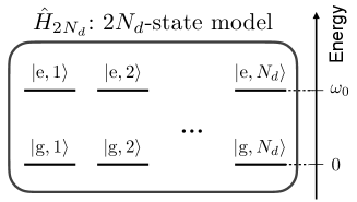
Figure 1: $2N_{d}$-state model introduced by Tajima and Funo

This system has $2N_{d}$ energy eigenstates in total. In this supplementary material, $N_{d}$ denotes the number of the excited states $\ket{\text{e},j}$, which is the same as the number of the ground states $\ket{\text{g},j}$. As we can see from the explicit form of the Hamiltonian $\hat{H}_{2N_{d}}$, the energy of the excited (ground) states is $\omega_{0}$ (0), where we set $\hbar=1$.

For the 2$N_{d}$-state model, Tajima and Funo assume the following interaction Hamiltonian $\hat{H}_{\text{int}}^{2N_{d}}$ between the $2N_{d}$-state system and environment:

$$\hat{H}_{\text{int}}^{2N_{d}}=\sum_{j,j^{\prime}=1}^{N_{d}}\left(\ket{\text{e},j}\!\bra{\text{g},j^{\prime}}\otimes\hat{B}+\ket{\text{g},j^{\prime}}\!\bra{\text{e},j}\otimes\hat{B}^{\dagger}\right),$$ (43)

where $\hat{B}$ denotes an operator acting on the environment. After taking the standard weak-coupling, Born-Markov, and rotating-wave approximations, the GKSL master equation for a quantum state $\hat{\rho}_{2N_{d}}(t)$ at time $t$ is given as follows:

$$\frac{d\hat{\rho}_{2N_{d}}(t)}{dt} =-i[\hat{H}_{2N_{d}},\hat{\rho}_{2N_{d}}(t)]+\mathcal{D}[\hat{\rho}_{2N_{d}}(t)],$$ (44)

$$\text{where}\ \mathcal{D}[\hat{\rho}]=\Gamma_{\downarrow}\left[\hat{L}\hat{\rho}\hat{L}^{\dagger}-\frac{1}{2}\{\hat{L}^{\dagger}\hat{L},\hat{\rho}\}\right]+\Gamma_{\uparrow}\left[\hat{L}^{\dagger}\hat{\rho}\hat{L}-\frac{1}{2}\{\hat{L}\hat{L}^{\dagger},\hat{\rho}\}\right].$$ (45)

Specifically, they define a collective Lindblad operator $\hat{L}$ as

$$\hat{L}=\sum_{j=1}^{N_{d}}\sum_{j^{\prime}=1}^{N_{d}}\ket{\text{g},j}\!\bra{\text{e},j^{\prime}},$$ (46)

which generates a collective energy decay of the system. Also, they assume that a detailed balance condition between the transition rates as $\Gamma_{\downarrow}/\Gamma_{\uparrow}=e^{\beta\omega_{0}}$.

III.2 Performance of $2N_{d}$-state model

Under these definitions introduced above, Tajima and Funo studied how the performance scales with the degeneracy $N_{d}$. For an sd state (defined as Eq. (9)) of the $2N_{d}$-state model, they obtain the following scaling of performance:

$$\text{For an sd state:}\ \frac{P}{\Delta\eta}=\Theta(N_{d}).$$ (47)

On the other hand, they also investigate a bd state (defined as Eq. (8)), and obtain

$$\text{For a bd state:}\ \frac{P}{\Delta\eta}=\Theta(N_{d}^{2}).$$ (48)

From the above results Eq. (47) and Eq. (48), they demonstrate a scaling enhancement of the heat engine performance. Importantly, they firstly reveal that a quantum coherence among degenerate states can be utilized to enhance the scaling with the degeneracy $N_{d}$ (See FIG. 2. for an abstract schematic of the scaling enhancement).

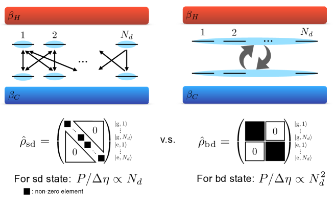
Figure 2: Scaling of the performance with the degeneracy $N_{d}$ of the 2$N_{d}$-state model discussed by Tajima and Funo

III.3 Comparison with results by Tajima and Funo

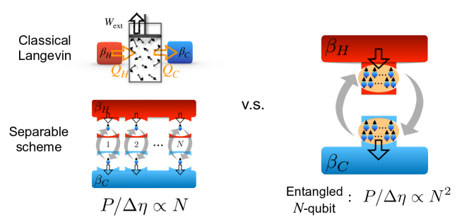
Figure 3: Scaling enhancement of the performance based on superabsorption. Unlike the 2$N_{d}$-state model by Tajima and Funo, we investigate how the performance scales not with the number of degeneracy $N_{d}$ but with the number of qubits $N$. As a result, we can compare our entangled scheme not only with the separable scheme, but also with the classical Langevin system.

Here, we compare the work done by Tajima and Funo with ours (See Table 1 and Table 2, respectively). The parameter with which Tajima and Funo study the scaling is the the number of degeneracy $N_{d}$, and they evaluate the scaling of performance for the two quantum states, the strictly diagonal (sd) state and the block-diagonal (bd) state (cf. FIG. 2). Meanwhile, as discussed in detail in the main text, we study the scaling with the number of qubits $N$, and we compare the performance for the entangled $N$-qubit system (i.e. entangled scheme) with that for a heat engine where we use $N$-qubit separable states as the working media (i.e. separable scheme). As a result, we obtain the performance $P/\Delta\eta=\Theta(N^{2})$ for the entangled scheme, and this exceeds the scaling for the separable scheme with $P/\Delta\eta=\Theta(N)$. Also, we can compare our result for the entangled scheme with a classical heat engine performance $P/\Delta\eta=\Theta(N)$ for $N$ particles obeying a Langevin equation, and we clearly see the scaling advantage beyond such classical heat engines as well (cf. FIG. 3)

One might think that our model and results can be reproduced by an appropriate interpretation of the $2N_{d}$-state model by Tajima and Funo. However, it is not the case. We have to notice that the Dicke states $\ket{1/2}$ and $\ket{-1/2}$ (composing the E2LS in the main text) are equal-weight superposition states of roughly $2^{N}/\sqrt{N}$-degenerated states, which is understood by a Stirling formula $n!\simeq\sqrt{2\pi n}\left(\frac{n}{e}\right)^{n}$. Thus, if we could naively adopt the result by Tajima and Funo, the performance by the E2LS would scale as $P/\Delta\eta=\Theta\left(\left(2^{N}/\sqrt{N}\right)^{2}\right)=\Theta(2^{2N}/N)$. However, this does not coincide with our result $P/\Delta\eta=\Theta(N^{2})$. We can understand the apparently different two models and their results in a unified point of view as follows.

First, regarding the model of Tajima and Funo, the system-environment interaction is described as the interaction Hamiltonian in Eq. (43). The jump operator $\hat{L}$ in Eq. (46) is exactly the same as the system operator of the interaction Hamiltonian, where information of the environment is embedded only in the correlation function $\Gamma_{\downarrow(\uparrow)}$. In their enhanced heat engine, they consider a subspace that is spanned by the following two equal-weight superposition states ($\ket{\text{e},+}$ and $\ket{\text{g},+}$) of degenerate quantum states:

$$\ket{\text{e},+} =\frac{1}{\sqrt{N_{d}}}\sum_{j=1}^{N_{d}}\ket{\text{e},j}, \ket{\text{g},+} =\frac{1}{\sqrt{N_{d}}}\sum_{j=1}^{N_{d}}\ket{\text{g},j}.$$ (49)

Then, the transition rate between these two states under the GKSL master equation is given by the square of the absolute value of the matrix element $\bra{\text{g},+}\hat{L}\ket{\text{e},+}$. This element explicitly reads

$$\bra{\text{g},+}\hat{L}\ket{\text{e},+} =\left[\frac{1}{\sqrt{N_{d}}}\Bigl{(}\bra{\text{g},1}+\cdots+\bra{\text{g},N_{d}}\Bigr{)}\right]\sum_{k,k^{\prime}=1}^{N_{d}}\ket{\text{g},k}\!\bra{\text{e},k^{\prime}}\left[\frac{1}{\sqrt{N_{d}}}\Bigl{(}\ket{\text{e},1}+\cdots+\ket{\text{e},N_{d}}\Bigr{)}\right]$$ (50)

$$=\frac{1}{N_{d}}\Bigl{(}\bra{\text{g},1}+\cdots+\bra{\text{g},N_{d}}\Bigr{)}\sum_{k,k^{\prime}=1}^{N_{d}}\ket{\text{g},k}\!\bra{\text{e},k^{\prime}}\Bigl{(}\ket{\text{e},1}+\cdots+\ket{\text{e},N_{d}}\Bigr{)}$$ (51)

Here, by the definition of the interaction Hamiltonian, the jump operator $\hat{L}$ connects one single excited state $\ket{\text{e},j^{\prime}}$ to every single ground state $\ket{\text{g},j}$, which one can see from $\bra{\text{g},j}\hat{L}\ket{\text{e},j^{\prime}}=1$ for all $(j,j^{\prime})$. This relation reflects the specific feature of the model of Tajima and Funo; in their model, the number of possible relaxation (excitation) processes from one single excited (ground) state to ground (excited) states, which we call the connectivity, is given by $N_{d}$. Because we obtain $N_{d}$ for one single excited state $\ket{\text{e},j^{\prime}}$ from the right parentheses, then, we obtain

$$\bra{\text{g},+}\hat{L}\ket{\text{e},+} =\frac{1}{N_{d}}\Bigl{(}\underbrace{N_{d}}_{\ket{\text{e},1}}+\underbrace{N_{d}}_{\ket{\text{e},2}}+\cdots+\underbrace{N_{d}}_{\ket{\text{e},N_{d}}}\Bigr{)}=\frac{1}{N_{d}}\times N_{d}\times N_{d}=N_{d}.$$ (52)

Thus, the square of the absolute value of this matrix element provides us the transition rate between $\ket{\text{e},+}$ and $\ket{\text{g},+}$, which is proportional to $N_{d}^{2}$. This leads to the scaling $\Theta(N_{d}^{2})$ of the speed of dynamics, and the enhanced heat engine performance $P/\Delta\eta=\Theta(N_{d}^{2})$.

On the other hand, in our system, the subspace under consideration is spanned by the two Dicke states $\ket{1/2}$ and $\ket{-1/2}$. The Dicke state $\ket{1/2}$ ($\ket{-1/2}$) is an equal-weight superposition state of all the $N$-qubit computational bases having $\frac{N+1}{2}$ $\left(\frac{N-1}{2}\right)$ qubits in the excited state $\ket{\text{e}}$ and the other $\frac{N-1}{2}$ $\left(\frac{N+1}{2}\right)$ qubits in the ground state $\ket{\text{g}}$ (cf. $N$: odd):

$$\left|\frac{1}{2}\right\rangle =\frac{1}{\sqrt{{}_{N}C_{(N+1)/2}}}\sum_{\text{all configuration}}|\{\underbrace{\text{e}\cdots\text{e}}_{\frac{N+1}{2}}\underbrace{\text{g}\cdots\text{g}}_{\frac{N-1}{2}}\}\rangle, \left|-\frac{1}{2}\right\rangle =\frac{1}{\sqrt{{}_{N}C_{(N+1)/2}}}\sum_{\text{all configuration}}|\{\underbrace{\text{e}\cdots\text{e}}_{\frac{N-1}{2}}\underbrace{\text{g}\cdots\text{g}}_{\frac{N+1}{2}}\}\rangle.$$ (53)

In our system, the system-environment interaction Hamiltonian contains the operator $\hat{J}_{\pm}=\sum_{i=1}^{N}\hat{\sigma}_{\pm}^{(i)}$ of the system. Thus, the relevant matrix element is $\bra{-1/2}\hat{J}_{-}\ket{1/2}$, which is explicitly given by

$$\bra{-1/2}\hat{J}_{-}\ket{1/2} =\left(\frac{1}{\sqrt{{}_{N}C_{(N+1)/2}}}\sum_{\text{a.c.}}\bra{\{\underbrace{\text{e}\cdots\text{e}}_{\frac{N-1}{2}}\underbrace{\text{g}\cdots\text{g}}_{\frac{N+1}{2}}\}}\right)\sum_{i=1}^{N}\hat{\sigma}_{-}^{(i)}\left(\frac{1}{\sqrt{{}_{N}C_{(N+1)/2}}}\sum_{\text{a.c.}}\ket{\{\underbrace{\text{e}\cdots\text{e}}_{\frac{N+1}{2}}\underbrace{\text{g}\cdots\text{g}}_{\frac{N-1}{2}}\}}\right)$$ (54)

$$=\frac{1}{{}_{N}C_{(N+1)/2}}\left(\sum_{\text{a.c.}}\bra{\{\underbrace{\text{e}\cdots\text{e}}_{\frac{N-1}{2}}\underbrace{\text{g}\cdots\text{g}}_{\frac{N+1}{2}}\}}\right)\sum_{i=1}^{N}\hat{\sigma}_{-}^{(i)}\left(\sum_{\text{a.c.}}\ket{\{\underbrace{\text{e}\cdots\text{e}}_{\frac{N+1}{2}}\underbrace{\text{g}\cdots\text{g}}_{\frac{N-1}{2}}\}}\right).$$ (55)

To get an intuitive idea of this calculation, we write down the transition from the specific computational basis $\ket{\text{eeegg}}$ for $N=5$:

$$\ket{\text{eeegg}}\xrightarrow{\hat{J}_{-}}\ket{\text{eeggg}}+\ket{\text{egegg}}+\ket{\text{geegg}}.$$ (56)

We have a superposition of three computational basis states. The number “3” of the flipped states comes from the number of the excited states (in the initial state $\ket{\text{eeegg}}$), which we can flip by the operator $\hat{J}_{-}$. Going back to Eq. (55) and taking one single computational basis $\ket{\{\underbrace{\text{e}\cdots\text{e}}_{\frac{N+1}{2}}\underbrace{\text{g}\cdots\text{g}}_{\frac{N-1}{2}}\}}$ in the right parentheses, we have $\frac{N+1}{2}$ excited states $\ket{\text{e}}$ to flip to the ground states $\ket{\text{g}}$ and obtain nonzero matrix elements $\left(\text{cf.}\ \frac{N+1}{2}=3\ \text{for}\ N=5\right)$. Then, we can calculate the matrix element $\bra{-1/2}\hat{J}_{-}\ket{1/2}$ as

$$\bra{-1/2}\hat{J}_{-}\ket{1/2} =\frac{1}{{}_{N}C_{(N+1)/2}}\Biggl{(}\underbrace{\frac{N+1}{2}+\frac{N+1}{2}+\cdots+\frac{N+1}{2}}_{{}_{N}C_{(N+1)/2}\ \text{terms}}\Biggr{)}=\frac{1}{{}_{N}C_{(N+1)/2}}\times{}_{N}C_{(N+1)/2}\times\frac{N+1}{2}$$ (57)

$$=\frac{N+1}{2}.$$ (58)

Thus, the square of the absolute value of this matrix element leads to the transition rate between $\ket{1/2}$ and $\ket{-1/2}$, which is proportional to $a_{1/2}=\frac{1}{4}(N+1)^{2}$.

Combining the results for the model of Tajima and Funo and ours, we can see the similarity between these two, which is illustrated in a simple form as follows:

$$(\text{matrix element})=\frac{1}{(\text{ normalization factor })^{2}}\times\text{(number of degeneracy)}\times(\text{connectivity})=(\text{connectivity}),$$ (59)

where we use the fact that the square of the normalization factor of an equally-weight superposition state is equivalent to the number of degeneracy. Therefore, we can conclude that the crucial factor leading to the enhanced scaling of performance is not the degeneracy in general; rather the connectivity remains after the calculation of the matrix element, and its square results in the scaling of the transition rates, or equivalently, the scaling of power. Incidentally, this importance of the connectivity was not so clear in the paper by Tajima and Funo, because, in their model, the number of degeneracy coincides with the connectivity, and we cannot easily distinguish these two independent contributions to the scaling of the matrix element. Taking this unified point of view, we can understand both the results of Tajima and Funo and ours, and we can get an insight into how to enhance the scaling of heat engine performance in general settings. Specifically, in order to obtain the enhanced scaling for a quantum heat engine, we have to implement a system-environment interaction that induces a large number of possible transitions between one degenerate subspace and another.

Table 1: Tajima Funo model

Parameter of scaling	$N_{d}$: number of degeneracy
Scheme with sd state	$P/\Delta\eta=\Theta(N_{d})$
Scheme with bd state	$P/\Delta\eta=\Theta(N^{2}_{d})$
Comparison	sd state v.s. bd state

Table 2: Our model

Parameter of scaling	$N$: number of qubits
Separable scheme	$P/\Delta\eta=\Theta(N)$
Classical counterpart	Langevin system: $P/\Delta\eta=\Theta(N)$
Scheme with entangled states	$P/\Delta\eta=\Theta(N^{2})$
Comparison	separable scheme (or Langevin sys.) v.s. entangled scheme

IV Experimental realization

Here, we explain a possible physical realization of our scheme using superconducting flux qubits. Superconducting qubits are artificial atoms with significant design freedoms Clarke and Wilhelm (2008). Especially, a superconducting flux qubit is composed of a superconducting loop interrupted by Josephson junctions. When we change the parameters of the circuit, we can design suitable properties of the flux qubits. For example, we can tune the qubit frequency and coupling strength by using magnetic flux through the SQUID embedded in the flux qubit Paauw et al. (2009); Zhu et al. (2010); Harris et al. (2010a, b). Moreover, the flux qubit can be strongly coupled with a microwave cavity Abdumalikov Jr et al. (2008); Yamamoto et al. (2014); Lindström et al. (2007); Johansson et al. (2006); Chiorescu et al. (2004). There are experimental demonstrations that an ensemble of the flux qubits is coupled with the microwave cavity Macha et al. (2014); Kakuyanagi et al. (2016). A long coherence time of around 90 ms is achieved Yan et al. (2016); Bylander et al. (2011); Abdurakhimov et al. (2019). Also, a technique to realize a coupling between the superconducting qubits via airbridged microwave cavity is reported Mukai et al. (2020), and this is useful to couple distant qubits. The cavity lifetime can be as long as a milli second Reagor et al. (2016), and we can decrease the cavity lifetime depending on the purpose Sevriuk et al. (2019). The coupling strength between the flux qubit and cavity can be as large as a few GHz Yoshihara et al. (2017) while the typical frequency of the flux qubit is also a few GHz. Also, the coupling between the flux qubit can be as large as a few GHz Harris et al. (2010a, b). These properties are prerequisite to realize our scheme.

In our proposed scheme, we consider 2$N$ flux qubits. We assume that $N$ flux qubits are coupled with an LC resonator (which we call a cavity A) that is coupled with a low-temperature thermal bath, while the other flux qubits are coupled with a different LC resonator (which we call a cavity B) that is coupled with a high-temperature thermal bath Johansson et al. (2006). We can couple the $N$ flux qubits with the other $N$ flux qubits via a transmission line resonator Lindström et al. (2007); Macha et al. (2014). Since the transmission line can be as large as a few cm, the temperature of the bath coupled with the cavity A could be different from that coupled with the cavity B. We can perform SWAP gates between the flux qubits by using the transmission line resonator, and this allows us to couple quantum states either a high temperature bath or low temperature bath Blais et al. (2004).

Our scheme can be implemented with the flux qubits as follows. First, we thermalize the $N$ flux qubits coupled with the cavity A. Second, we change the frequency of the flux qubits at the cavity A, and swap the quantum state of the qubits coupled with the cavity A to the one coupled with the cavity B. Third, we thermalize the $N$ qubits at the cavity B. Fourth, we change the frequency of the flux qubits at the cavity B, and swap the quantum state of the qubits coupled with the cavity B to that coupled with the cavity A. Finally, we repeat these four steps.

In the numerical calculations shown in FIG.2 in the main text, we assume that the frequency of the flux qubits is $\omega_{A}^{H}/2\pi=1$ GHz. Then, the coupling strength $\Omega/2\pi$ between the qubits is equal to 31 MHz. By setting the coupling strength between the transmission line resonator and the flux qubits to be around 100 MHz, we can perform the swap gates within a few nano seconds. During the thermalization processes, the cavity-qubit coupling $g/2\pi$ is around $10^{-5}\times\omega_{A}^{H}/2\pi=$10 kHz, and the thermalization period $\tau_{H}$ and $\tau_{C}$ is around 10 nano seconds when $N=9$, while the coherence time of the flux qubits can be as long as 90 ms. Thus, we can ignore the decoherence of the flux qubits except that induced by the cavity A and B. The temperature inside the dilution refrigerator can be as small as 10 mK, and the temperature $T_{H}=(k_{B}\beta_{H})^{-1}$ and $T_{C}=(k_{B}\beta_{C})^{-1}$ we assume are respectively given by 20 mK and 10 mK.

References

- Tajima and Funo (2021) H. Tajima and K. Funo, Phys. Rev. Lett. 127, 190604 (2021).
- Shiraishi et al. (2016) N. Shiraishi, K. Saito, and H. Tasaki, Phys. Rev. Lett. 117, 190601 (2016).
- Streltsov et al. (2017) A. Streltsov, G. Adesso, and M. B. Plenio, Rev. Mod. Phys. 89, 041003 (2017).
- Higgins et al. (2014) K. Higgins, S. Benjamin, T. Stace, G. Milburn, B. W. Lovett, and E. Gauger, Nat. Commun. 5, 1 (2014).
- Clarke and Wilhelm (2008) J. Clarke and F. K. Wilhelm, Nature 453, 1031 (2008).
- Paauw et al. (2009) F. Paauw, A. Fedorov, C. M. Harmans, and J. Mooij, Phys. Rev. Lett. 102, 090501 (2009).
- Zhu et al. (2010) X. Zhu, A. Kemp, S. Saito, and K. Semba, Appl. Phys. Lett. 97, 102503 (2010).
- Harris et al. (2010a) R. Harris, M. W. Johnson, T. Lanting, A. Berkley, J. Johansson, P. Bunyk, E. Tolkacheva, E. Ladizinsky, N. Ladizinsky, T. Oh, et al., Phys. Rev. B 82, 024511 (2010a).
- Harris et al. (2010b) R. Harris, J. Johansson, A. Berkley, M. Johnson, T. Lanting, S. Han, P. Bunyk, E. Ladizinsky, T. Oh, I. Perminov, et al., Phys. Rev. B 81, 134510 (2010b).
- Abdumalikov Jr et al. (2008) A. A. Abdumalikov Jr, O. Astafiev, Y. Nakamura, Y. A. Pashkin, and J. Tsai, Phys. Rev. B 78, 180502 (2008).
- Yamamoto et al. (2014) T. Yamamoto, K. Inomata, K. Koshino, P. Billangeon, Y. Nakamura, and J. Tsai, New J. Phys. 16, 015017 (2014).
- Lindström et al. (2007) T. Lindström, C. Webster, J. Healey, M. Colclough, C. Muirhead, and A. Y. Tzalenchuk, Supercond. Sci. Technol. 20, 814 (2007).
- Johansson et al. (2006) J. Johansson, S. Saito, T. Meno, H. Nakano, M. Ueda, K. Semba, and H. Takayanagi, Phys. Rev. Lett. 96, 127006 (2006).
- Chiorescu et al. (2004) I. Chiorescu, P. Bertet, K. Semba, Y. Nakamura, C. Harmans, and J. Mooij, Nature 431, 159 (2004).
- Macha et al. (2014) P. Macha, G. Oelsner, J.-M. Reiner, M. Marthaler, S. André, G. Schön, U. Hübner, H.-G. Meyer, E. Il’ichev, and A. V. Ustinov, Nat. Commun. 5, 1 (2014).
- Kakuyanagi et al. (2016) K. Kakuyanagi, Y. Matsuzaki, C. Déprez, H. Toida, K. Semba, H. Yamaguchi, W. J. Munro, and S. Saito, Phys. Rev. Lett. 117, 210503 (2016).
- Yan et al. (2016) F. Yan, S. Gustavsson, A. Kamal, J. Birenbaum, A. P. Sears, D. Hover, T. J. Gudmundsen, D. Rosenberg, G. Samach, S. Weber, et al., Nat. Commun. 7, 1 (2016).
- Bylander et al. (2011) J. Bylander, S. Gustavsson, F. Yan, F. Yoshihara, K. Harrabi, G. Fitch, D. G. Cory, Y. Nakamura, J.-S. Tsai, and W. D. Oliver, Nat. Phys. 7, 565 (2011).
- Abdurakhimov et al. (2019) L. V. Abdurakhimov, I. Mahboob, H. Toida, K. Kakuyanagi, and S. Saito, Appl. Phys. Lett. 115, 262601 (2019).
- Mukai et al. (2020) H. Mukai, K. Sakata, S. J. Devitt, R. Wang, Y. Zhou, Y. Nakajima, and J.-S. Tsai, New J. Phys. 22, 043013 (2020).
- Reagor et al. (2016) M. Reagor, W. Pfaff, C. Axline, R. W. Heeres, N. Ofek, K. Sliwa, E. Holland, C. Wang, J. Blumoff, K. Chou, et al., Phys. Rev. B 94, 014506 (2016).
- Sevriuk et al. (2019) V. Sevriuk, K. Y. Tan, E. Hyyppä, M. Silveri, M. Partanen, M. Jenei, S. Masuda, J. Goetz, V. Vesterinen, L. Grönberg, et al., Appl. Phys. Lett. 115, 082601 (2019).
- Yoshihara et al. (2017) F. Yoshihara, T. Fuse, S. Ashhab, K. Kakuyanagi, S. Saito, and K. Semba, Nat. Phys. 13, 44 (2017).
- Blais et al. (2004) A. Blais, R.-S. Huang, A. Wallraff, S. M. Girvin, and R. J. Schoelkopf, Phys. Rev. A 69, 062320 (2004).