Generalizing the Constant-roll Condition in Scalar Inflation

Abstract

In this work we generalize the constant-roll condition for minimally coupled canonical scalar field inflation. Particularly, we shall assume that the scalar field satisfies the condition $\ddot{\phi}=\alpha(\phi)V^{\prime}(\phi)$, and we derive the field equations under this assumption. We call the framework extended constant-roll framework. Accordingly we calculate the inflationary indices and the corresponding observational indices of inflation. In order to demonstrate the inflationary viability, we choose three potentials that are problematic in the context of slow-roll dynamics, namely chaotic, linear power-law and exponential inflation, and by choosing a simple power-law form for the smooth function $\alpha(\phi)$, we show that in the extended constant-roll framework, the models are compatible with the latest 2018 Planck constraints on inflation. We also justify appropriately why we called this new framework extended constant-roll framework, and we show that the condition $\ddot{\phi}=\alpha(\phi)V^{\prime}(\phi)$ is equivalent to the condition $\ddot{\phi}=\beta(\phi)H\dot{\phi}$, with the latter condition being a simple generalization of the constant-roll condition. Finally, we examine an interesting physical situation, in which a general extended constant-roll scalar field model is required to satisfy the cosmological tracker condition used in quintessence models. In contrast to the slow-roll and ordinary constant-roll cases, in which case the tracker condition is not compatible with neither the slow-roll or the ordinary constant-roll conditions, the extended constant-roll condition can be compatible with the tracker condition. This feature leads to a new inflationary phenomenological framework, the essential features of which we develop in brief. The main feature of the new theoretical framework is that the function $\alpha(\phi)$ and the potential $V(\phi)$ are no longer free to choose, but these are directly functionally related.

I Introduction

The most common description of the inflationary era is materialized by a canonical minimally coupled scalar field Guth:1980zm ; Starobinsky:1982ee ; Linde:1983gd ; Albrecht:1982wi , called inflaton. To date, it has not be verified that inflation ever took place primordially, nevertheless inflation solves smoothly many theoretical inconsistencies of the standard cosmological model, thus it remains the most appealing candidate for the description of the primordial post-Planck era, with the most promising alternative class of theories being modified gravity theories Nojiri:2017ncd ; Nojiri:2010wj ; Nojiri:2006ri ; Capozziello:2011et ; Capozziello:2010zz ; delaCruzDombriz:2012xy ; Olmo:2011uz . Nowadays, the latest Planck data Akrami:2018odb impose stringent constraints on the inflationary parameters, and it seems that the power-spectrum of the primordial curvature perturbations is nearly scale invariant. The standard scalar field description of inflation assumes that the scalar field slowly rolls down its potential, however during the last decades, several alternative descriptions like the constant-roll case Inoue:2001zt ; Tsamis:2003px ; Kinney:2005vj ; Tzirakis:2007bf ; Namjoo:2012aa ; Martin:2012pe ; Motohashi:2014ppa ; Cai:2016ngx ; Motohashi:2017aob ; Hirano:2016gmv ; Anguelova:2015dgt ; Cook:2015hma ; Kumar:2015mfa ; Odintsov:2017yud ; Odintsov:2017qpp ; Lin:2015fqa ; Gao:2017uja ; Nojiri:2017qvx ; Oikonomou:2017bjx ; Odintsov:2017hbk ; Oikonomou:2017xik ; Cicciarella:2017nls ; Awad:2017ign ; Anguelova:2017djf ; Ito:2017bnn ; Karam:2017rpw ; Yi:2017mxs ; Mohammadi:2018oku ; Gao:2018tdb ; Mohammadi:2018wfk ; Morse:2018kda ; Cruces:2018cvq ; GalvezGhersi:2018haa ; Boisseau:2018rgy ; Gao:2019sbz ; Lin:2019fcz have been studied in the literature. In this paper we aim to generalize the constant-roll condition in such a way so that $\ddot{\phi}=\alpha(\phi)V^{\prime}(\phi)$, where $\alpha(\phi)$ is some smooth function of the scalar field, and we call this framework the extended constant-roll framework. We develop the extended constant-roll framework and derive expressions for the inflationary indices and for the observational indices of inflation, focusing on the spectral index of the scalar perturbations and on the tensor-to-scalar ratio. In order to examine the viability of the resulting framework, we choose three popular inflationary models, which in the slow-roll inflation are problematic, namely the chaotic inflation, the linear power-law and the exponential inflation models. As we show, for a simple power-law choice of the smooth function $\alpha(\phi)$, the three models are in good agreement with the Planck data. Also we explain why we named the condition $\ddot{\phi}=\alpha(\phi)V^{\prime}(\phi)$ as extended constant-roll condition, since this condition is equivalent to $\ddot{\phi}=\beta(\phi)H\dot{\phi}$, by employing a simple transformation. Finally, we demonstrate that the imposition of the tracker condition is compatible with the extended constant-roll scenario, a feature of the theoretical framework we developed, which can play an important role for the unified description of inflation with the dark energy era, by using a single scalar field.

For the rest of the study, we shall use a flat Friedman-Robertson-Walker (FRW) spacetime, with its line element being,

$$ds^{2}=-dt^{2}+a(t)^{2}\sum_{i=1,2,3}\left(dx^{i}\right)^{2}\,,$$ (1)

where $a(t)$ is as usual the scale factor.

II Extended Constant-roll: Formalism and Applications

We shall consider minimally coupled scalar field cosmology, with the action being,

$$\mathcal{S}=\int d^{4}x\left(\frac{R}{2\kappa^{2}}-\frac{1}{2}\partial_{\mu}\phi\partial^{\mu}\phi-V(\phi)\right)\,,$$ (2)

where $\kappa^{2}=\frac{1}{M_{p}^{2}}$ where $M_{p}$ is the reduced Planck mass. The field equations corresponding to the above action are,

$$\centering 3H^{2}=\kappa^{2}\left(\frac{1}{2}\dot{\phi}^{2}+V\right)\,,\@add@centering$$ (3)

$$\centering-2\dot{H}=\kappa^{2}\dot{\phi}^{2}\,,\@add@centering$$ (4)

$$\centering\ddot{\phi}+3H\dot{\phi}+V^{\prime}=0\,.\@add@centering$$ (5)

The slow-roll indices for a minimally coupled scalar theory are Hwang:2005hb ,

$$\epsilon_{1}=-\frac{\dot{H}}{H^{2}},$$ (6)

$$\epsilon_{2}=\frac{\ddot{\phi}}{H\dot{\phi}},$$

and the observational indices for the inflationary theory, namely the spectral index of scalar perturbations $n_{s}$ and the tensor-to-scalar ratio are Nojiri:2017ncd ; Hwang:2005hb ,

$$n_{s}=1-4\epsilon_{1}-2\epsilon_{2}\,,$$ (7)

$$r=\frac{8\kappa^{2}Q_{s}}{f_{R}}\,,$$ (8)

where $Q_{s}=\frac{\dot{\phi}^{2}}{H^{2}}$. In view of the Raychaudhuri equation (4) we get $Q_{s}=-\frac{2\dot{H}}{\kappa^{2}H^{2}}$, therefore, the tensor-to-scalar ratio reads,

$$r=16\epsilon_{1}\,.$$ (9)

The extended constant-roll condition we shall consider in this work is the following,

$$\ddot{\phi}=\alpha(\phi)V^{\prime}(\phi)\,,$$ (10)

where $\alpha(\phi)$ is a smooth dimensionless function of the scalar field $\phi$. In view of the extended constant-roll condition (10), the equation of motion for the scalar field (5) yields,

$$\dot{\phi}=-\frac{V^{\prime}(\phi)\left(1+\alpha(\phi)\right)}{3H}\,.$$ (11)

Now assuming the standard slow-roll condition for the scalar field, namely,

$$\frac{\dot{\phi}^{2}}{2}\ll V(\phi)\,,$$ (12)

the Friedmann equation yields as usual,

$$\frac{3H^{2}}{\kappa^{2}}\simeq V(\phi)\,,$$ (13)

and upon combining Eqs. (11) and (13), the slow-roll indices (14) take the following compact forms,

$$\epsilon_{1}=\frac{1}{2\kappa^{2}}\left(\frac{V^{\prime}}{V}\right)^{2}\left(1+\alpha(\phi)\right)^{2},\,\,\,\epsilon_{2}=-\frac{3\alpha(\phi)}{1+\alpha(\phi)}\,.$$ (14)

The effect of the extended constant-roll condition is apparent on the slow-roll indices, since $\epsilon_{2}$ becomes independent of the potential, and the first slow-roll index depends explicitly on $\alpha(\phi)$. Obviously, the standard constant-roll condition can be obtained by considering $\alpha(\phi)=\mathrm{const}$, but we shall extensively discuss this issue in a later section because there exists a symmetry which can directly connect the extended constant-roll condition (10) with the standard constant-roll condition. Let us proceed in finding the expression for the $e$-foldings number for the case of the extended constant-roll scenario, and we easily find by using Eq. (11) that,

$$N=\int_{\phi_{i}}^{\phi_{f}}\frac{H}{\dot{\phi}}d\phi=\kappa^{2}\int_{\phi_{f}}^{\phi_{i}}\frac{V}{V^{\prime}}\frac{1}{\left(1+\alpha(\phi)\right)}d\phi\,,$$ (15)

where $\phi_{i}$ is the value of the scalar field at the first horizon crossing primordially during the first stages of inflation, and $\phi_{f}$ is the value of the scalar field at the end of the inflationary era. Having Eqs. (7), Eqs. (9), Eqs. (14), and Eqs. (15), we can directly test several cosmological scalar field models and confront the inflationary phenomenology they produce with the 2018 Planck data Akrami:2018odb . In the next subsections we shall consider three scalar field models which without the extended constant-roll condition are not compatible with the 2018 Planck data, and thus phenomenologically excluded. As we shall demonstrate, in the context of the extended constant-roll scenario, these models become compatible with the Planck observational constraints.

Before we close, let us in brief quote the formulas that yield the predicted non-Gaussianities, just for the sake of completeness. For the models studied in the next section, the predicted non-Gaussianities are not reportable because these are quite small. The formula that yields the equilateral parameter $f_{NL}^{equil}$ can be found in Ref. DeFelice:2011zh , and it is using their notation,

$$f_{NL}^{equil}=\frac{11}{56}\epsilon_{1}+\frac{5}{12}\eta\,,$$ (16)

where $\eta=\frac{\dot{\epsilon}_{1}}{H\epsilon_{1}}$. In our notation, the relation that connects $\eta$ and the slow-roll indices $\epsilon_{1}$ and $\epsilon_{2}$ can easily be found by using the equations of motion, and this is,

$$\epsilon_{2}=\frac{\ddot{H}}{2H\dot{H}}=-\epsilon_{1}+\frac{\dot{\epsilon}_{1}}{2\epsilon_{1}H}\,,$$ (17)

or equivalently,

$$\eta=2\left(\epsilon_{1}+\epsilon_{2}\right)\,.$$ (18)

Hence, the equilateral parameter $f_{NL}^{eqil}$ can be written in terms of the slow-roll indices $\epsilon_{1}$ and $\epsilon_{2}$ as follows,

$$f_{NL}^{equil}=\frac{55}{36}\epsilon_{1}+\frac{10}{12}\left(\epsilon_{1}+\epsilon_{2}\right)\,.$$ (19)

II.1 Chaotic, Linear and Exponential Inflation Phenomenology with the Extended Constant-roll Condition

We shall apply the extended constant-roll formalism we developed previously in the case of chaotic inflation scenario Linde:1983gd which was quite popular in the 80’s and 90’s but it is not viable with respect to the Planck data. As we now show, by choosing a simple power law form for the dimensionless function $\alpha(\phi)$, the chaotic inflation model can become compatible with observations.

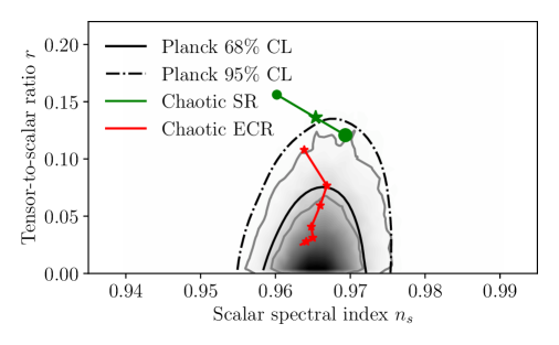
Figure 1: The extended constant-roll chaotic inflation scenario (red lines and points Extended Constant-roll (ECR)) versus the ordinary slow-roll chaotic inflation scenario (green lines and points, Slow-roll (SR)), in view of the Planck 2018 data.

The chaotic inflation scenario has the following scalar potential Linde:1983gd $V(\phi)=\frac{V_{0}}{\kappa^{4}}\left(\kappa\phi\right)^{2}$, where $V_{0}$ is the dimensionless potential multiplication factor. The upper value of $\frac{V_{0}}{\kappa^{4}}$ is determined by the latest Planck data, but it is irrelevant for our analysis, so we do not discuss this issue further. The dimensionless function $\alpha(\phi)$ entering in the extended constant-roll condition (10) shall be chosen as $\alpha(\phi)=\delta\left(\kappa\phi\right)^{m}-1$ The slow-roll indices can easily be calculated for the above choices and these are $\epsilon_{1}=2\delta^{2}\kappa^{2m-2}\phi^{2m-2}$, $\epsilon_{2}=\frac{3\kappa^{-m}\phi^{-m}}{\delta}-3$. We can find the value of the scalar field at the end of inflation $\phi_{f}$, by solving the equation $\epsilon_{1}(\phi_{f})=\mathcal{O}(1)$, and accordingly, by performing the integration (15), we obtain the value of the scalar field at first horizon crossing $\phi_{i}$, so these two are $\phi_{f}=\frac{2^{\frac{1}{2-2m}}\delta^{\frac{1}{1-m}}}{\kappa}$, $\phi_{i}=2^{\frac{1}{2-m}}\delta^{\frac{1}{2-m}}\kappa^{-1}\left(2^{\frac{m}{2-2m}}\delta^{\frac{1}{1-m}}+(m-2)N\right)$. The spectral index of the scalar curvature perturbations $n_{s}$ and the tensor-to-scalar ratio $r$ acquire the following simple forms in terms of the scalar field, $n_{s}=-8\delta^{2}\kappa^{2m-2}\phi^{2m-2}-\frac{6\kappa^{-m}\phi^{-m}}{\delta}+7$, and $r=32\delta^{2}\kappa^{2m-2}\phi^{2m-2}$. By evaluating the slow-roll indices at first horizon crossing, thus for the scalar field taking the value $\phi_{i}$ quoted above, we can easily confront this model with the Planck 2018 observational data. The results of our analysis are presented in Fig. 1. The free parameters values are in the ranges $\delta=10^{-5}-10^{-19}$ and $m=4-12$, for $N=60$ $e$-foldings, and the extended constant-roll chaotic inflation model corresponds to the red lines and points in Fig. 1. We have also included in Fig. 1 the ordinary chaotic inflation model with green lines and points. Obviously, the extended constant-roll chaotic inflation model is well fitted with the Planck 2018 data, in contrast to the ordinary chaotic inflation scenario.

Let us now consider the linear power-law inflation scenario, which has the following scalar potential, $V(\phi)=\frac{V_{0}}{\kappa^{4}}\kappa\phi$, where $V_{0}$ again as the dimensionless potential multiplication factor the value of is irrelevant for our analysis. The dimensionless function $\alpha(\phi)$ of the extended constant-roll condition (10) is again chosen as, $\alpha(\phi)=\delta\left(\kappa\phi\right)^{m}-1$. The slow-roll indices for the linear inflation model take the simple form $\epsilon_{1}=\frac{1}{2}\delta^{2}\kappa^{2m-2}\phi^{2m-2}$, and $\epsilon_{2}=\frac{3\kappa^{-m}\phi^{-m}}{\delta}-3$. As in the previous section, the values of the scalar field at the end of inflation $\phi_{f}$, and at horizon crossing $\phi_{i}$ are easily found to be, $\phi_{f}=\frac{2^{\frac{1}{2m-2}}\delta^{\frac{1}{1-m}}}{\kappa}$, $\phi_{i}=\left(2^{-\frac{m-2}{2(m-1)}}\delta^{\frac{m-2}{m-1}}\kappa^{m-2}+\delta(m-2)N\kappa^{m-2}\right)^{\frac{1}{2-m}}$. Accordingly, the observational indices take the following forms, $n_{s}=-2\delta^{2}\kappa^{2m-2}\phi^{2m-2}-\frac{6\kappa^{-m}\phi^{-m}}{\delta}+7$, and $r=8\delta^{2}\kappa^{2m-2}\phi^{2m-2}$. Upon evaluation of the observational indices at first horizon crossing, we can directly confront the model at hand with the Planck 2018 observational data. The results of our analysis for the linear power-law inflationary model are presented in Fig. 2. The free parameters values are taken in this case in the ranges $\delta=10^{-5}-10^{-17}$ and again $m=4-12$, for $N=60$ $e$-foldings. The extended constant-roll chaotic inflation model corresponds to the red lines and points in Fig. 2, while with yellow lines and points we presented the ordinary linear power-law slow-roll inflationary model which is known to be incompatible with the Planck data.

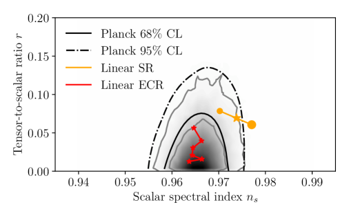
Figure 2: The extended constant-roll linear power-law inflation scenario (red lines and points Extended Constant-roll (ECR)) versus the ordinary slow-roll linear power-law inflation scenario (yellow lines and points, Slow-roll (SR)), in view of the Planck 2018 data.

Thus we demonstrated that for both the chaotic and linear power-law inflationary models, the extended constant-roll condition renders both viable inflationary models and compatible with the latest Planck data. In the same spirit as in the chaotic and linear inflation model, let us present in brief the resulting phenomenology of a model which fails to be compatible with the observational data in the standard slow-roll description. Let us consider the simple exponential model, with potential, $V(\phi)=\frac{V_{0}}{\kappa^{4}}\exp\left(\lambda\kappa\phi\right)$ where $\lambda$ is a dimensionless parameter. In this case we choose the dimensionless function $\alpha(\phi)$ to be, $\alpha(\phi)=\left(\kappa\phi\right)^{m}-1$, and note the absence of the parameter $\delta$ which was present in the previous two models. The results of our analysis for the exponential model are presented in Fig. 3. The free parameters values are in the ranges $\lambda=8.1\times 10^{-3}-10^{-3}$ and $m=4-12$, for $N=60$ $e$-foldings. The extended constant-roll exponential inflation model corresponds to the red lines and points in Fig. 3, where the bottom plot is a closeup of the upper plot. The slow-roll exponential model yields a constant slow-roll index $\epsilon_{1}$ and is quite problematic, however the extended constant-roll exponential model is compatible with the Planck data for all the values of the free parameters we used. As it can be seen, the model predicts inflation deeply in the Planck $95\%$ CL likelihood curve.

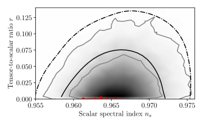
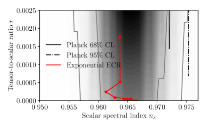
Figure 3: The extended constant-roll simple exponential inflation scenario (red lines and points) in view of the Planck 2018 data. The bottom plot is a closeup of the upper plot.

III Symmetries and Tracking Condition Framework

We have named the condition (10) as extended constant-roll condition, however we have not properly justified why we used the terminology extended constant-roll condition. The constant-roll condition is basically,

$$\ddot{\phi}=\beta H\dot{\phi}\,,$$ (20)

where $\beta$ is some constant number. Let us now see how our terminology extended constant-roll for the condition (10) is justified. Before we do that, let us present an alternative definition of the extended constant-roll condition, which can be materialized by the following condition,

$$\ddot{\phi}=\beta(\phi)H\dot{\phi}\,,$$ (21)

where $\beta(\phi)$ is some smooth dimensionless function of the scalar field $\phi$. The relation (21) is a direct generalization of the constant-roll condition (20), for $\beta(\phi)=\mathrm{const}$. In view of the extended constant-roll condition (21), the equation of motion for the scalar field (5) yields,

$$\dot{\phi}=-\frac{V^{\prime}(\phi)}{\left(3+\beta(\phi)\right)H}\,.$$ (22)

Now again assuming the standard slow-roll condition for the scalar field, namely Eq. (12) the Friedmann equation takes the form (13), hence by using Eqs. (22) and (13), the slow-roll indices (14) take the following compact forms in this case,

$$\epsilon_{1}=\frac{9}{2\kappa^{2}\left(3+\beta(\phi)\right)^{2}}\left(\frac{V^{\prime}}{V}\right)^{2}$$ (23)

$$\epsilon_{2}=\beta(\phi)\,.$$

Also, the $e$-foldings number for the case at hand, can easily be found by using Eq. (22) that,

$$N=\int_{\phi_{i}}^{\phi_{f}}\frac{H}{\dot{\phi}}d\phi=\kappa^{2}\int_{\phi_{f}}^{\phi_{i}}\frac{V}{3V^{\prime}}\left(3+\beta(\phi)\right)d\phi\,.$$ (24)

At this point we shall show how the terminology extended constant-roll is justified for the condition (10). Basically the inflationary phenomenologies related to the conditions (10) and (21) are directly related by using the following transformation,

$$\beta(\phi)\to-\frac{3\alpha(\phi)}{1+\alpha(\phi)}\,.$$ (25)

It is easy to see that the two phenomenologies are identical under the transformation (25), and this is why we used the terminology extended constant-roll for the condition (10), since the physics of this condition is identical to the physics of condition (21).

Before closing, it is worth mentioning an interesting perspective of the extended constant-roll scenario, related to tracking solutions Steinhardt:1999nw . Tracker fields or tracking attractor solutions were initially introduced in order to solve the coincidence problem in quintessence theories. Tracker fields have an equation of motion with attractor solutions which rapidly converge to a common universal attractor for a wide range of initial conditions. Tracker solutions are appealing due to the fact that the scalar field energy eventually overtakes the energy density of dark matter eventually at late times. An important condition in order to have tracking solutions is the following Steinhardt:1999nw ,

$$\frac{V^{\prime}}{V}=\frac{H}{\dot{\phi}}\,,$$ (26)

which is known as tracker condition. In a quintessence theory it would be desirable to describe with the same scalar field both early and late times. However as we now demonstrate, the tracker condition eventually destroys slow-roll dynamics. On the contrary, the tracker condition has some interesting physics to offer if it is considered in conjunction with the extended constant-roll condition. Let us consider first the standard slow-roll approach, in which case the following two conditions govern the dynamics of the scalar field,

$$\frac{\dot{\phi}^{2}}{2}\ll V,\,\,\,\ddot{\phi}\ll H\dot{\phi}\,.$$ (27)

In view of the standard slow-roll conditions (27), the equation of motion for the scalar field (5) yields,

$$V^{\prime}\simeq-3H\dot{\phi}\,.$$ (28)

The tracker condition (26) can be written as,

$$\frac{V^{\prime}}{V}=\frac{H\dot{\phi}}{\dot{\phi}^{2}}\,,$$ (29)

and since $V^{\prime}$ and $H\dot{\phi}$ are of the same order due to Eq. (28), Eq. (29) implies that $V$ and $\dot{\phi}^{2}$ are of the same order, which contradicts the first slow-roll condition of Eq. (27). Thus the tracker condition (26) is not compatible with the slow-roll evolution, and this indicate it is rather hard to describe with the same scalar field inflation and quintessence tracker solutions. The same conclusion can be obtained easily if we directly substitute Eq. (28) in Eq. (26), to obtain, $\frac{1}{2\kappa^{2}}\left(\frac{V^{\prime}}{V}\right)^{2}\simeq-\frac{1}{2}$, where we used that during slow-roll $3H^{2}\simeq\kappa^{2}V$.

Now let us demonstrate the implications of the tracker conditions on a single scalar field theory cosmology which evolves with the extended constant-roll condition holding true. In the extended constant-roll evolution, the term $\dot{\phi}$ is given by Eq. (11), thus upon substituting this in the tracker condition (26), we obtain,

$$\frac{3H^{2}V}{\left(V^{\prime}\right)^{2}}=-\left(1+\alpha(\phi)\right)\,,$$ (30)

or by using $3H^{2}=\kappa^{2}\,V$, and recalling the functional form of the first slow-roll index $\epsilon_{1}$ from Eq. (14), the tracker condition (26) is transformed to a condition for the slow-roll index $\epsilon_{1}$, which is,

$$\epsilon_{1}=-\frac{1+\alpha(\phi)}{2}\,.$$ (31)

Essentially the tracker condition constrains the forms of the potential in such a way so that the first slow-roll index $\epsilon_{1}$ takes the simple form (31). The second slow-roll index remains identical with the one appearing in Eq. (14), and what further changes is the final expression for the $e$-foldings number, which actually further constrains the functional form that $\alpha(\phi)$ can take. Actually, in view of the tracker condition (30), the $e$-foldings number expression (15) takes the following simple form,

$$N=\kappa\int_{\phi_{i}}^{\phi_{f}}\frac{d\phi}{\sqrt{-1-\alpha(\phi)}}\,,$$ (32)

with the constraint that $\alpha(\phi)+1<0$. In principle the tracker condition does not contradict scalar field cosmologies which satisfy the extended constant-roll condition. Thus basically the tracker condition in conjunction with the extended constant-roll condition, introduce a new class of inflationary phenomenology, which can combine both the tracking condition and the extended constant-roll conditions. This class of theory could be of importance if the unification of inflation with late-time acceleration is the aim of a theory. We have not further analyzed this newly introduced class of models, however, we aim to further develop these theories in a future work. Finally, let us briefly comment that even the constant-roll condition leads to problems if it is considered in conjunction with the tracker condition (26). Indeed, for $\ddot{\phi}=\beta H\dot{\phi}$ ($\beta$ recall is constant), the tracker condition in conjunction with the equation of motion of the scalar field yields $\epsilon_{1}=-\frac{3}{2}\frac{1}{3+\beta}$, which is not incompatible in general with the constant-roll condition. However this case is obviously problematic because both $\epsilon_{1}$ and $\epsilon_{2}$ are basically constants. Thus the inflationary phenomenology of the resulting theory is severely restricted, and no new insights are expected. On the contrary, the tracker condition in conjunction with the extended constant-roll condition may offer the possibility of having late-time evolution with a de Sitter equation of state parameter, and also describe inflation with the same theory. This issue will be addressed in a future work. Finally, let us note that in the context of the extended constant-roll framework considered in conjunction with the tracker condition, the scalar field potential and the scalar function $\alpha(\phi)$ are no longer freely chosen since these are connected by Eq. (14), so basically the potential $V(\phi)$ and the function $\alpha(\phi)$ must satisfy,

$$\kappa^{2}\left(\frac{V}{V^{\prime}}\right)^{2}=-(1+\alpha(\phi))\,.$$ (33)

IV Conclusions

In this paper we introduced the theoretical framework of extended constant-roll dynamics for minimally coupled single scalar field cosmologies. The extended constant-roll condition constrains basically the scalar field evolution which was required to satisfy the condition $\ddot{\phi}=\alpha(\phi)V^{\prime}(\phi)$. Accordingly we derived the corresponding field equations, and we calculated the inflationary indices and the corresponding observational indices of inflation, focusing on the spectral index of the primordial scalar curvature perturbations and the tensor-to-scalar ratio. Employing the new formalism by using a simple power-law $\alpha(\phi)$ function, we demonstrated that three otherwise problematic scalar potentials in the context of slow-roll inflation, become compatible with the latest Planck observational data in the context of the extended constant-roll framework. Particularly, we studied the chaotic inflation scenarios, an exponential potential and finally a linear power-law potential. The condition $\ddot{\phi}=\alpha(\phi)V^{\prime}(\phi)$ is equivalent to the condition $\ddot{\phi}=\beta(\phi)H\dot{\phi}$, which is a direct extension of the original constant-roll condition, for non-constant functions $\beta(\phi)$. Finally, we imposed an extra condition to be satisfied by the extended constant-roll scalar fields, namely the tracker condition. Originally the tracker condition was engineered for the quintessence scenario in order to explain the coincidence problem. As we showed, the extended constant-roll scenario is compatible with the tracker condition, and a new inflationary phenomenological framework arises with this new constraint, in contrast to the slow-roll and constant-roll cases, which lead to inconsistencies if the tracker condition is imposed. We briefly discussed how the inflationary phenomenology can be extracted with this new tracker condition constraints, the main feature of which is that the function $\alpha(\phi)$ and the potential $V(\phi)$ are directly functionally related. In a future work a compelling task would be to investigate whether the same scalar field can simultaneously describe inflation and the dark energy era, and we hope to address this issue in a future work.

References

- (1) A. H. Guth, Phys. Rev. D 23 (1981) 347. doi:10.1103/PhysRevD.23.347
- (2) A. A. Starobinsky, Phys. Lett. 91B (1980) 99. doi:10.1016/0370-2693(80)90670-X
- (3) A. D. Linde, Phys. Lett. 129B (1983) 177. doi:10.1016/0370-2693(83)90837-7
- (4) A. Albrecht and P. J. Steinhardt, Phys. Rev. Lett. 48 (1982) 1220 [Adv. Ser. Astrophys. Cosmol. 3 (1987) 158]. doi:10.1103/PhysRevLett.48.1220
- (5) S. Nojiri, S. D. Odintsov and V. K. Oikonomou, Phys. Rept. 692 (2017) 1 doi:10.1016/j.physrep.2017.06.001 [arXiv:1705.11098 [gr-qc]].
- (6) S. Nojiri and S. D. Odintsov, Phys. Rept. 505 (2011) 59 doi:10.1016/j.physrep.2011.04.001 [arXiv:1011.0544 [gr-qc]].
- (7) S. Nojiri and S. D. Odintsov, eConf C 0602061 (2006) 06 [Int. J. Geom. Meth. Mod. Phys. 4 (2007) 115] doi:10.1142/S0219887807001928 [hep-th/0601213].
- (8) S. Capozziello and M. De Laurentis, Phys. Rept. 509 (2011) 167 doi:10.1016/j.physrep.2011.09.003 [arXiv:1108.6266 [gr-qc]].
- (9) V. Faraoni and S. Capozziello, Fundam. Theor. Phys. 170 (2010). doi:10.1007/978-94-007-0165-6
- (10) A. de la Cruz-Dombriz and D. Saez-Gomez, Entropy 14 (2012) 1717 doi:10.3390/e14091717 [arXiv:1207.2663 [gr-qc]].
- (11) G. J. Olmo, Int. J. Mod. Phys. D 20 (2011) 413 doi:10.1142/S0218271811018925 [arXiv:1101.3864 [gr-qc]].
- (12) Y. Akrami et al. [Planck Collaboration], arXiv:1807.06211 [astro-ph.CO].
- (13) S. Inoue and J. Yokoyama, Phys. Lett. B 524 (2002) 15 doi:10.1016/S0370-2693(01)01369-7 [hep-ph/0104083].
- (14) N. C. Tsamis and R. P. Woodard, Phys. Rev. D 69 (2004) 084005 doi:10.1103/PhysRevD.69.084005 [astro-ph/0307463].
- (15) W. H. Kinney, Phys. Rev. D 72 (2005) 023515 doi:10.1103/PhysRevD.72.023515 [gr-qc/0503017].
- (16) K. Tzirakis and W. H. Kinney, Phys. Rev. D 75 (2007) 123510 doi:10.1103/PhysRevD.75.123510 [astro-ph/0701432].
- (17) M. H. Namjoo, H. Firouzjahi and M. Sasaki, Europhys. Lett. 101 (2013) 39001 doi:10.1209/0295-5075/101/39001 [arXiv:1210.3692 [astro-ph.CO]].
- (18) J. Martin, H. Motohashi and T. Suyama, Phys. Rev. D 87 (2013) no.2, 023514 doi:10.1103/PhysRevD.87.023514 [arXiv:1211.0083 [astro-ph.CO]].
- (19) H. Motohashi, A. A. Starobinsky and J. Yokoyama, JCAP 1509 (2015) no.09, 018 doi:10.1088/1475-7516/2015/09/018 [arXiv:1411.5021 [astro-ph.CO]].
- (20) Y. F. Cai, J. O. Gong, D. G. Wang and Z. Wang, JCAP 1610 (2016) no.10, 017 doi:10.1088/1475-7516/2016/10/017 [arXiv:1607.07872 [astro-ph.CO]].
- (21) H. Motohashi and A. A. Starobinsky, arXiv:1702.05847 [astro-ph.CO].
- (22) S. Hirano, T. Kobayashi and S. Yokoyama, Phys. Rev. D 94 (2016) no.10, 103515 doi:10.1103/PhysRevD.94.103515 [arXiv:1604.00141 [astro-ph.CO]].
- (23) L. Anguelova, Nucl. Phys. B 911 (2016) 480 doi:10.1016/j.nuclphysb.2016.08.020 [arXiv:1512.08556 [hep-th]].
- (24) J. L. Cook and L. M. Krauss, JCAP 1603 (2016) no.03, 028 doi:10.1088/1475-7516/2016/03/028 [arXiv:1508.03647 [astro-ph.CO]].
- (25) K. S. Kumar, J. Marto, P. Vargas Moniz and S. Das, JCAP 1604 (2016) no.04, 005 doi:10.1088/1475-7516/2016/04/005 [arXiv:1506.05366 [gr-qc]].
- (26) S. D. Odintsov and V. K. Oikonomou, arXiv:1703.02853 [gr-qc].
- (27) S. D. Odintsov and V. K. Oikonomou, arXiv:1704.02931 [gr-qc].
- (28) J. Lin, Q. Gao and Y. Gong, Mon. Not. Roy. Astron. Soc. 459 (2016) no.4, 4029 doi:10.1093/mnras/stw915 [arXiv:1508.07145 [gr-qc]].
- (29) Q. Gao and Y. Gong, arXiv:1703.02220 [gr-qc].
- (30) S. Nojiri, S. D. Odintsov and V. K. Oikonomou, Class. Quant. Grav. 34 (2017) no.24, 245012 doi:10.1088/1361-6382/aa92a4 [arXiv:1704.05945 [gr-qc]].
- (31) V. K. Oikonomou, Mod. Phys. Lett. A 32 (2017) no.33, 1750172 doi:10.1142/S0217732317501723 [arXiv:1706.00507 [gr-qc]].
- (32) S. D. Odintsov, V. K. Oikonomou and L. Sebastiani, Nucl. Phys. B 923 (2017) 608 doi:10.1016/j.nuclphysb.2017.08.018 [arXiv:1708.08346 [gr-qc]].
- (33) V. K. Oikonomou, Int. J. Mod. Phys. D 27 (2017) no.02, 1850009 doi:10.1142/S0218271818500098 [arXiv:1709.02986 [gr-qc]].
- (34) F. Cicciarella, J. Mabillard and M. Pieroni, JCAP 1801 (2018) no.01, 024 doi:10.1088/1475-7516/2018/01/024 [arXiv:1709.03527 [astro-ph.CO]].
- (35) A. Awad, W. El Hanafy, G. G. L. Nashed, S. D. Odintsov and V. K. Oikonomou, JCAP 1807 (2018) no.07, 026 doi:10.1088/1475-7516/2018/07/026 [arXiv:1710.00682 [gr-qc]].
- (36) L. Anguelova, P. Suranyi and L. C. R. Wijewardhana, JCAP 1802 (2018) no.02, 004 doi:10.1088/1475-7516/2018/02/004 [arXiv:1710.06989 [hep-th]].
- (37) A. Ito and J. Soda, Eur. Phys. J. C 78 (2018) no.1, 55 doi:10.1140/epjc/s10052-018-5534-5 [arXiv:1710.09701 [hep-th]].
- (38) A. Karam, L. Marzola, T. Pappas, A. Racioppi and K. Tamvakis, JCAP 1805 (2018) no.05, 011 doi:10.1088/1475-7516/2018/05/011 [arXiv:1711.09861 [astro-ph.CO]].
- (39) Z. Yi and Y. Gong, JCAP 1803 (2018) no.03, 052 doi:10.1088/1475-7516/2018/03/052 [arXiv:1712.07478 [gr-qc]].
- (40) A. Mohammadi, K. Saaidi and T. Golanbari, Phys. Rev. D 97 (2018) no.8, 083006 doi:10.1103/PhysRevD.97.083006 [arXiv:1801.03487 [hep-ph]].
- (41) Q. Gao, Y. Gong and Q. Fei, JCAP 1805 (2018) no.05, 005 doi:10.1088/1475-7516/2018/05/005 [arXiv:1801.09208 [gr-qc]].
- (42) A. Mohammadi and K. Saaidi, arXiv:1803.01715 [astro-ph.CO].
- (43) M. J. P. Morse and W. H. Kinney, Phys. Rev. D 97 (2018) no.12, 123519 doi:10.1103/PhysRevD.97.123519 [arXiv:1804.01927 [astro-ph.CO]].
- (44) D. Cruces, C. Germani and T. Prokopec, JCAP 1903 (2019) no.03, 048 doi:10.1088/1475-7516/2019/03/048 [arXiv:1807.09057 [gr-qc]].
- (45) J. T. Galvez Ghersi, A. Zucca and A. V. Frolov, JCAP 1905 (2019) no.05, 030 doi:10.1088/1475-7516/2019/05/030 [arXiv:1808.01325 [astro-ph.CO]].
- (46) B. Boisseau and H. Giacomini, arXiv:1809.09169 [gr-qc].
- (47) Q. Gao, Y. Gong and Z. Yi, arXiv:1901.04646 [gr-qc].
- (48) W. C. Lin, M. J. P. Morse and W. H. Kinney, arXiv:1904.06289 [astro-ph.CO].
- (49) J. c. Hwang and H. Noh, Phys. Rev. D 71 (2005) 063536 doi:10.1103/PhysRevD.71.063536 [gr-qc/0412126].
- (50) A. De Felice and S. Tsujikawa, JCAP 1104 (2011) 029 doi:10.1088/1475-7516/2011/04/029 [arXiv:1103.1172 [astro-ph.CO]].
- (51) P. J. Steinhardt, L. M. Wang and I. Zlatev, Phys. Rev. D 59 (1999), 123504 doi:10.1103/PhysRevD.59.123504 [arXiv:astro-ph/9812313 [astro-ph]].