Manifold Matching via Deep Metric Learning for Generative Modeling

Abstract

We propose a manifold matching approach to generative models which includes a distribution generator (or data generator) and a metric generator. In our framework, we view the real data set as some manifold embedded in a high-dimensional Euclidean space. The distribution generator aims at generating samples that follow some distribution condensed around the real data manifold. It is achieved by matching two sets of points using their geometric shape descriptors, such as centroid and $p$-diameter, with learned distance metric; the metric generator utilizes both real data and generated samples to learn a distance metric which is close to some intrinsic geodesic distance on the real data manifold. The produced distance metric is further used for manifold matching. The two networks learn simultaneously during the training process. We apply the approach on both unsupervised and supervised learning tasks: in unconditional image generation task, the proposed method obtains competitive results compared with existing generative models; in super-resolution task, we incorporate the framework in perception-based models and improve visual qualities by producing samples with more natural textures. Experiments and analysis demonstrate the feasibility and effectiveness of the proposed framework.

1 Introduction

Deep generative models including Variational Autoencoder (VAE) [21], Generative Adversarial Networks (GAN) [13] and their variants [3, 26, 24, 42, 10, 55, 41] have achieved great success in generative tasks such as image and video synthesis, super-resolution (SR), image-to-image translation, text generation, neural rendering, etc. The above approaches try to generate samples which mimic real data by minimizing various discrepancies between their corresponding statistical distributions, such as using KL divergence [21], Jensen-Shannon divergence [13], Wasserstein distance [3], Maximum Mean Discrepancy [26] and so on. These approaches focused on the data distribution aspect and did not pay enough attention to the underlying metrics of these distributions. The interplay between distribution measure and its underlying metric is a central topic in optimal transport (cf. [47]). Despite that researchers have successfully employed optimal transport theory in generative models [3, 50, 9], simply assuming the underlying metric to be Euclidean metric may neglect some rich information lying in the data [1]. In addition, although the above approaches are validated to be effective, successful training setups are mostly based on empirical observations and lack of physical interpretations.

In this paper we bring up a geometric perspective which serves as an important parallel view of generative models as GANs. Table 1 summarizes the main differences between classic GANs and our proposed (so-called MvM) framework. Instead of directly matching statistical discrepancies under Euclidean distance, we provide a more flexible framework which is built upon learning the intrinsic distances among data points. Specifically, we treat the real data set as some manifold embedded in high-dimensional Euclidean space, and generate a fake distribution measure condensed around the real data manifold by optimizing a Manifold Matching (MM) objective. The MM objective is built on shape descriptors, such as centroid and $p$-diameter with respect to some proper metric learnt by a metric generator using Metric Learning (ML) approaches. During training process, the (fake data) distribution generator and the metric generator work interchangeably and produces better distribution (metric) that facilitates the efficient training of metric (distribution) generator. The learned distances can not only be used to formulate energy-based loss functions [22] for MM, but can also reveal meaningful geometric structures of real data manifold.

Table 1: Main differences between GANs and MvM.

Differences	GANs	MvM
Main point of view	statistics	geometry
Matching terms	means, moments, etc.	centroids, $p$-diameters
Matching criteria	statistical discrepancy	learned distances
Underlying metric	default Euclidean	learned intrinsic
Objective functions	one min-max value function	two distinct objectives

We apply the proposed framework on two tasks: unconditional image generation and single image super-resolution (SISR). We utilize unconditional image generation task as a validation of the feasibility of the approach; and further implement a supervised version of the framework on SISR task to demonstrate its advantage. Our main contributions are: (1) We propose a manifold matching approach for generative modeling, which matches geometric descriptors between real and generated data sets using distances learned during training; (2) We provide a flexible framework for modeling data and building objectives, where each generator has its own designated objective function; (3) We conduct experiments on unconditional image generation task and SISR task which validates the effectiveness of the proposed framework.

2 Related Work

Manifold Matching: Shen et al. [45] proposed a nonlinear manifold matching algorithm using shortest-path distance and joint neighborhood selection, and illustrated its usage in medical imaging applications. Priebe et al. [39] investigated in manifold matching task from the perspective of jointly optimizing the fidelity and commensurability, with an application in document matching. Lim and Ye [28] decomposed GAN training into three geometric steps and used SVM separating hyperplane that has the maximal margins between classes. Lei et al. [25] showed the intrinsic relations between optimal transportation and convex geometry, and further used it to analyze generative models. Genevay et al. [12] introduced the Sinkhorn loss in generative models, based on regularized optimal transport with an entropy penalty. Shao et al. [44] introduced ways of exploring the Riemannian geometry of manifolds learned by generative models, and showed that the manifolds learned by deep generative models are close to zero curvature. Park et al. [38] added a manifold matching loss in GAN objectives which tried to match distributions using kernel tricks. However, the learning process highly relies on optimizing objectives in the original GAN framework. In addition, without proper metrics, using pre-defined kernels may fail to match the true shapes of data manifolds. In our work, the manifold matching is implemented using geometric descriptors under proper metrics learned by a metric generator.

Deep Metric Learning: Among rich sources of literature on deep metric learning, we mainly focus on a few that are related to our work. Xing et al. [51] first proposed distance metric learning with applications to improve clustering performance. Hoffer and Ailon implemented deep metric learning with Triplet network [18] which aimed to learn useful representations through distance comparisons. Duan et al. [11] proposed a deep adversarial metric learning framework to generate synthetic hard negatives from negative samples. The hard negative generator and feature embedding were trained simultaneously to learn more precise distance metrics. The metrics were learned in a supervised fashion and then used in classification tasks. Unlike [11], our approach utilizes geometric descriptors for matching data manifolds to generate data without using any labelled information. Mohan et al. [37] proposed a direction regularization method which tried to improve the representation space being learnt by guiding the pairs move towards right directions in the metric space. In this work, we utilize the approach in [37] for metric learning implementation,

Perception-Based SISR: SISR aims to recover a high-resolution (HR) image from a low-resolution (LR) one. Ledig et al. [23] first incorporated adversarial component in their objective and achieved high perceptual quality. However, SRGAN can generate observable artifacts such as undesirable noise and whitening effect. Similar issues were also mentioned in Sajjadi et al. [43]. Wang et al. [48] proposed ESRGAN which improved perceptual quality by improving SRGAN network architecture and combining PSNR-oriented network and a GAN-based network to balance perceptual quality and fidelity. Ma et al. [31] proposed a gradient branch which provides additional structure priors for the SR process. Utilization of the gradient branch need corresponding network architectures to be equipped with. Soh et al. [46] introduced natural manifold discriminator which tried to distinguish real and generated noisy and blurry samples. Since the natural manifold discriminator focuses on classifying certain types of manually generated fake data, one following question is: can we find a more robust way to learn useful information from real data? Thus in this case we view one usage of our work in SR task as an extension of the natural manifold discriminator. Some other recent methods [27, 8, 40, 29, 16, 6] mainly work on improving network architectures which are not directly comparable to our approach. In this paper we focus on objectives regardless of generator architectures, while the method can be incorporated into existing works.

3 Methodology

3.1 Proposed Framework

We propose a metric measure framework for generative modeling which contains a distribution generator $f_{\theta}:\mathbb{R}^{m}\rightarrow\mathbb{R}^{D}$ and a metric generator $g_{w}:\mathbb{R}^{D}\rightarrow\mathbb{R}^{n}$.

$$\mathbb{R}^{m}\xrightarrow{\hskip 8.5359ptf_{\theta}\hskip 8.5359pt}\mathbb{R}^{D}\xrightarrow{\hskip 8.5359ptg_{w}\hskip 8.5359pt}\mathbb{R}^{n}$$

The metric generator $g_{w}$ would produce some metric $d$ on $\mathbb{R}^{D}$ to be the pullback of the Euclidean metric $d_{E}$ on $\mathbb{R}^{n}$ (see Definition 3.2). The distribution generator $f_{\theta}$ would produce some measure $\mu$ on $\mathbb{R}^{D}$ to be the pushforward of some prior distribution $\nu$ on $\mathbb{R}^{m}$ (see Definition 3.1). In implementations, $m,D,n$ represent dimensions of the input variable, target image, and image embedding respectively.

Now we have a metric measure space $(\mathbb{R}^{D},d,\mu)$. The space of real data is viewed as some manifold $M\subseteq\mathbb{R}^{D}$ embedded in Euclidean space. The measure $\mu$ is said to be condensed around manifold $M$ if the majority of the measure $\mu$ is distributed nearby $M$ (see Fig. 1). The manifold $M$ is called totally geodesic (or “straight”) with respect to metric $d$ if for any two points $a,b\in M$, the shortest path measured by metric $d$ stays on $M$ (see Fig. 2). Using the generators $f_{\theta}$, $g_{w}$ modeled as neural networks, we aim to find proper parameters $\theta$ and $w$ such that the induced measure $\mu$ and metric $d$ satisfies:
(1) $\mu$ is as condensed as possible around $M$;
(2) $M$ is as “straight” as possible under $d$.

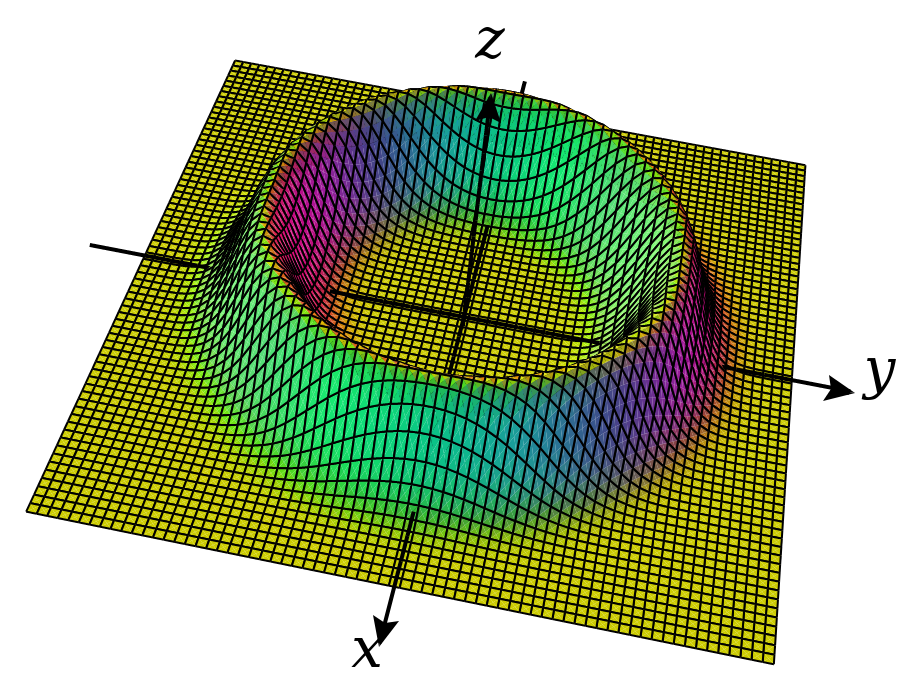
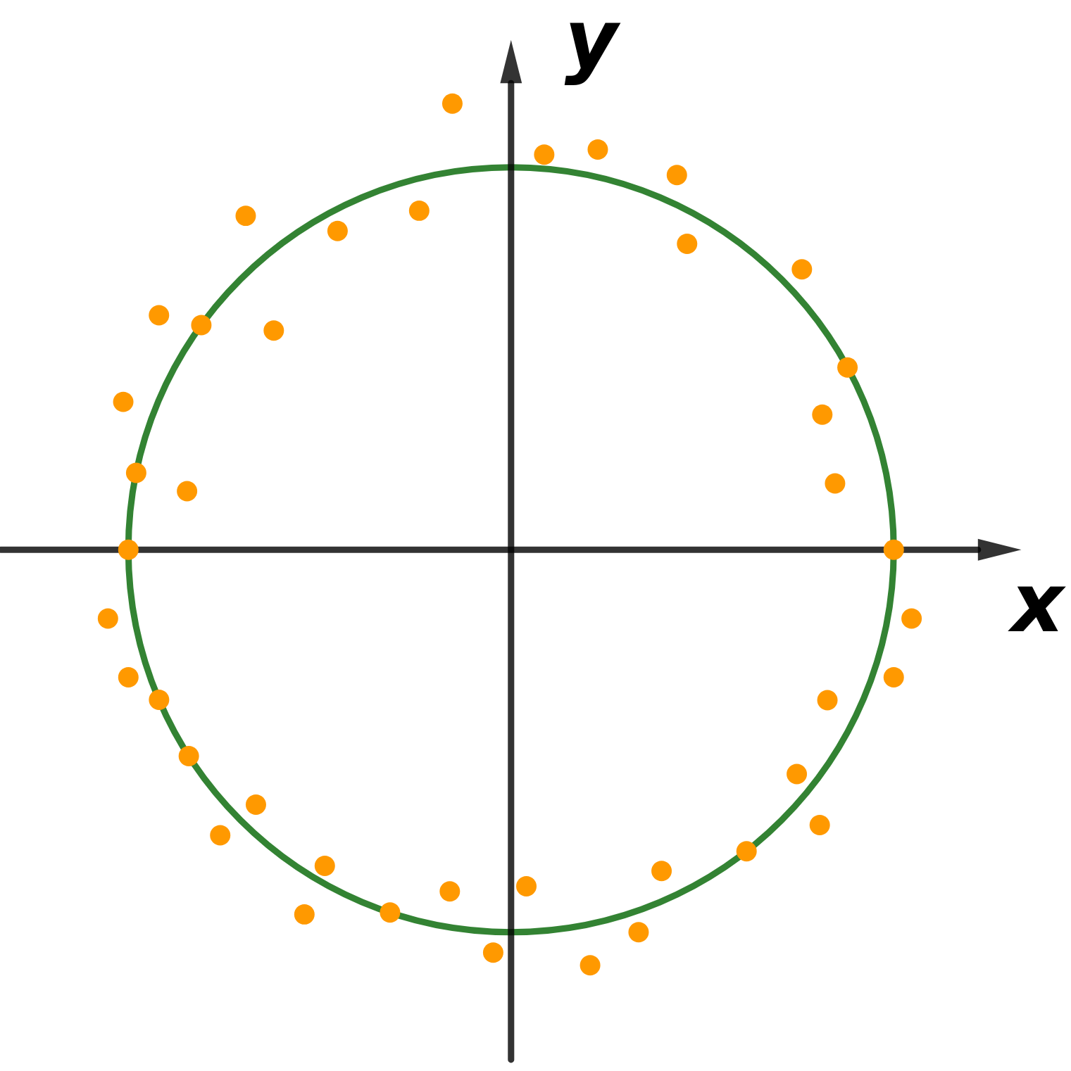
(i)	(ii)

Figure 1: (i) The probability density function of a distribution $\mu$ which condensed around a circle (manifold) $M\subseteq\mathbb{R}^{2}$; (ii) The orange dots represents random samples of $\mu$ and the green circle represents the real data manifold $M\subseteq\mathbb{R}^{2}$.

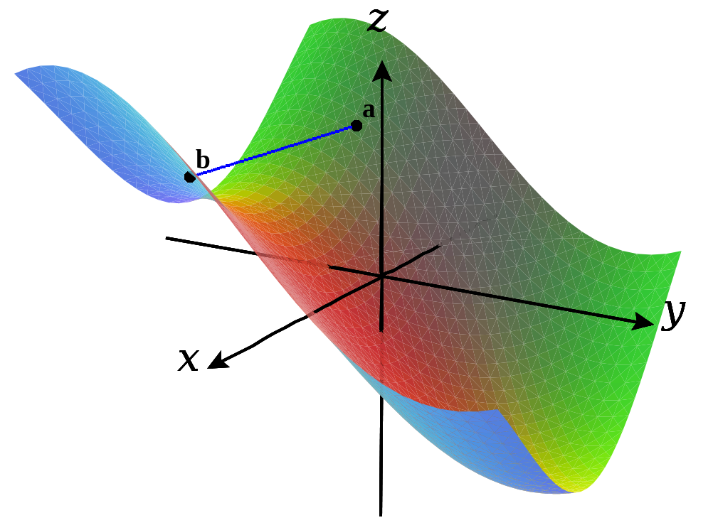
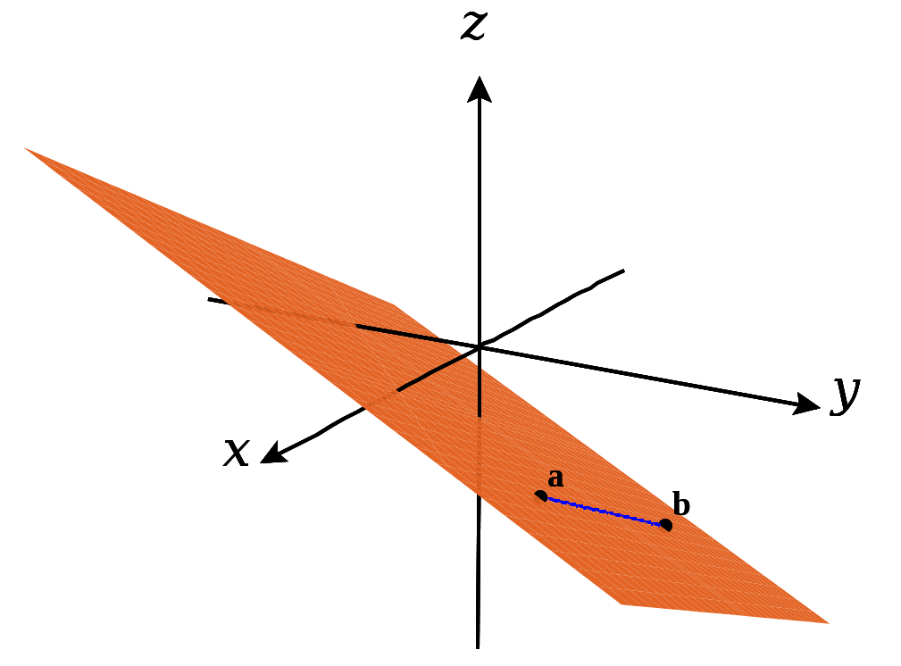
(i)	(ii)

Figure 2: The blue segment represents the shortest path between two points $a,b$ with respect to Euclidean distance $d_{E}$. (i) A non-geodesic sub-manifold of $\mathbb{R}^{3}$ under $d_{E}$; (ii) A geodesic sub-manifold of $\mathbb{R}^{3}$ under $d_{E}$.

Generally speaking, the two networks would produce a sequence of metrics $\{d_{2i}\}_{i\geq 0}$ and a sequence of measures $\{\mu_{2i+1}\}_{i\geq 0}$ inductively and alternatively as follows: (i) Let $d_{0}=d_{E}$; Then for any $i>0$, (ii) derive measure $\mu_{2i-1}$ using manifold matching based on metric $d_{2i-2}$; (iii) derive metric $d_{2i}$ using metric learning based on measure $\mu_{2i-1}$.

$$d_{0}=d_{E}\rightsquigarrow\mu_{1}\rightsquigarrow d_{2}\rightsquigarrow\mu_{3}\rightsquigarrow d_{4}\rightsquigarrow\cdots$$

In the following we introduce how to implement manifold matching and metric learning in details.

3.2 Manifold Matching

Let $\mathcal{P}(X)$ be the set of all probability measures on space $X$. Let $\mathcal{D}(X)$ be the set of all metrics on space $X$.

Definition 3.1 (Pushforward measure).

Given a map $f:X\rightarrow Y$ and a probability measure $\mu\in\mathcal{P}(X)$, the push forward measure $f_{\ast}(\mu)\in\mathcal{P}(Y)$ is defined as: for any measurable set $A\subseteq Y$,

$$(f_{\ast}\mu)(A):=\mu(f^{-1}(A)).$$

Definition 3.2 (Pullback metric).

Given a map $g:Y\rightarrow Z$ and a metric $d\in\mathcal{D}(Z)$, the pull back metric $g^{\ast}(d)\in\mathcal{D}(Y)$ is defined as: for any $y_{1},y_{2}\in Y$,

$$(g^{\ast}d)(y_{1},y_{2}):=d(g(y_{1}),g(y_{2})).$$

Manifold matching in our work refers to finding parameter $\theta_{0}$ of a specific generative network $f_{\theta}:\mathbb{R}^{m}\rightarrow\mathbb{R}^{D}$ such that the pushforward $(f_{\theta_{0}})_{\ast}\nu$ of some prior distribution $\nu$ via $f_{\theta_{0}}$ is condensed around a manifold $M\subseteq\mathbb{R}^{D}$. In our case, the real data manifold $M\subseteq\mathbb{R}^{D}$ generally has no explicit expression. In other words, given a point $a\in\mathbb{R}^{D}$ these is no way to explicitly tell whether $a\in M$ or how far away $a$ is from $M$. For this reason, we attempt to estimate the shape of $M$ via a set of sample points from $M$.

The centroid of a space is an important descriptor of its shape. For a metric measure space, the Fréchet mean (cf. [14, 7, 4]) is a natural generalization of the centroid:

Definition 3.3 (Fréchet mean).

The Fréchet mean set $\sigma(\mathcal{X})$ of a metric measure space $\mathcal{X}=(X,d,\mu)$ is defined as

$$\underset{x\in X}{\operatorname{arg\,min}}\int_{X}d^{2}(x,y)d\mu(y).$$

The Fréchet mean roughly informs the center of $\mathcal{X}$, but to reach the goal of manifold matching, we also need a shape descriptor indicating the size of $\mathcal{X}$. Hence we introduce the notion of $p$-diameter [34]:

Definition 3.4 ($p$-diameter).

For any $p\geq 1$, the $p$-diameter of metric measure space $\mathcal{X}:=(X,d,\mu)$ is defined as

$$\operatorname{diam}_{p}(\mathcal{X}):=\left(\int_{X}\int_{X}d(x,x^{\prime})^{p}d\mu(x)d\mu(x^{\prime})\right)^{1/p}.$$

The above definitions of Fréchet mean and $p$-diameter are for metric measure spaces, but it also applies to any manifold assuming a uniform volume measure on it. Let $S:=\{x_{1},x_{2},\cdots,x_{k}\}$ be a sequence of independent identically distributed points sampled from $\mu$. Let $\mu_{k}=\frac{1}{k}\Sigma_{i=1}^{k}\delta_{x_{i}}$ denote the empirical measure. We can estimate the shape of $(X,d,\mu)$ by the shape of $(S,d|_{S},\mu_{k})$. In the following we simply denote $\sigma(S):=\sigma(S,d|_{S},\mu_{k})$ and $\operatorname{diam}_{p}(S):=\operatorname{diam}_{p}(S,d|_{S},\mu_{k})$.

When to estimate the $p$-diameter, if $p$ is relatively large, $\operatorname{diam}_{p}(S)$ is very sensitive to the outliers. To ensure a trustworthy estimation, we choose $p=2$ and use $\operatorname{diam}_{2}$ as a size indicator.

Let $S_{R}$ be a set of random real data samples of $M$ and $S_{F}$ be a set of random fake data samples of $\mu=(f_{\theta})_{\ast}\nu$. Then the objective function we propose for manifold matching is:

$$L_{MM}:= d\big{(}\sigma(S_{R}),\sigma(S_{F})\big{)}+$$

$$\lambda\big{|}\operatorname{diam}_{2}(S_{R})-\operatorname{diam}_{2}(S_{F})\big{|},$$ (1)

where $\lambda$ is a weight parameter.

3.3 Metric Learning

Shape descriptors for manifold matching greatly rely on a proper choice of metric $d$. Although in most cases Euclidean metric $d_{E}$ is easy to access, it may not be an intrinsic choice and barely reveals the actual shape of a data set. The intrinsic metric on a Riemannian manifold $M$ is specified by geodesic distance. Specifically, the geodesic distance between two points on the manifold equals the length of shortest path on $M$ which connects them. From this point of view, a better choice of metric on the ambient space $\mathbb{R}^{D}\supseteq M$ should make the shortest path connecting $a,b\in M$ stay as close as possible to $M$, or in other words, make $M$ as “straight” as possible. Here we apply Triplet metric learning to learn a proper metric on $\mathbb{R}^{D}$:

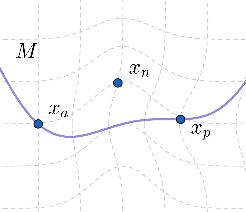
Figure 3: Minimizing the Triplet loss pushes out negative sample $x_{n}$ and pulls back positive sample $x_{p}$. As a result, the learned metric would “distort” the space and “straighten” the manifold.

Definition 3.5.

Given a triple $(x_{a},x_{p},x_{n})$ with $x_{a},x_{p}\in M$ and $x_{n}\notin M$, the Triplet loss is defined as

$$L_{tri}:=\max\{0,d^{2}(x_{a},x_{p})-d^{2}(x_{a},x_{n})+\alpha\}.$$

Here $d=(g_{w})^{\ast}d_{E}$ and $\alpha$ is a margin parameter. People usually call $x_{a}$ an anchor sample, $x_{p}$ a positive sample and $x_{n}$ a negative sample.

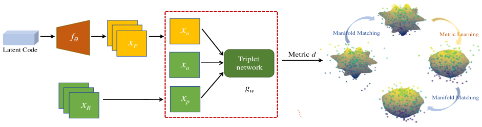
Figure 4: Implementation pipeline of the proposed MvM framework. $x_{R}$ and $x_{F}$ represent samples in real data set $S_{R}$ and generated data set $S_{F}$, respectively. The distribution generator $f_{\theta}$ outputs samples $x_{F}\in S_{F}$ based on manifold matching criteria under learned metric. For Triplet metric learning, anchor samples $x_{a}$ and positive samples $x_{p}$ are randomly selected from $S_{R}$, and negative samples $x_{n}$ are randomly selected from $S_{F}$, without labelled data involved in this step. Learned distance metric is then used for manifold matching. Manifold matching step makes the fake samples (dots) condense around the real data manifold (surface), while metric learning step tries to “straighen” or “flatten” the real data manifold. These two steps goes interchangeably until convergence.

By minimizing $L_{tri}$, we attempt to pull back the positive sample to anchor and push out the negative sample, only when $d(x_{a},x_{p})$ is relatively larger than $d(x_{a},x_{n})$. Fig. 3 illustrates how this would “straighten” the manifold.

Among numerous methods for metric learning, in our implementation we choose one recent approach [37] which adapted Triplet loss by adding a direction regularizer to make the metric learned towards right direction. Hence in our paper the Triplet loss becomes:

$$L_{apn} =\max\{0,d^{2}(x_{a},x_{p})-d^{2}(x_{a},x_{n})+\alpha-$$

$$\gamma Cos(g_{w}(x_{n})-g_{w}(x_{a}),g_{w}(x_{p})-g_{w}(x_{a}))\},$$ (2)

where $\gamma$ is the direction guidance parameter which controls the magnitude of regularization applied to the original Triplet loss $L_{tri}$. In practice one can also employ other methods to learn proper distance metrics.

3.4 Objective Functions

In the metric learning community, the metric generator $g_{w}$ is usually viewed as a metric embedding. From this point of view we have (see supplement for the proof):

Proposition 3.6.

Given two measure $\mu_{1}$ and $\mu_{2}$ on the same metric space $(X,d)$, where $d=g^{\ast}d_{E}$. Then $d\left(\sigma(X,d,\mu_{1}),\sigma(X,d,\mu_{2})\right)=d_{E}(\overline{g_{\ast}\mu_{1}},\overline{g_{\ast}\mu_{2}})$.

Let $\|\cdot\|$ denote $L^{2}$ norm and $d=(g_{w})^{\ast}d_{E}$, then we have $d(x,x^{\prime})=\|g_{w}(x)-g_{w}(x^{\prime})\|$ for $\forall x,x^{\prime}\in\mathbb{R}^{D}$. By above proposition, the explicit formula of terms in our objective functions (3.2) are as follows:

$$d\big{(}\sigma(S_{R}),\sigma(S_{F})\big{)}=\|\overline{g_{w}(S_{R})}-\overline{g_{w}(S_{F})}\|,$$

$$\operatorname{diam}_{2}(S)=\frac{1}{card(S)}\left(\sum_{x,x^{\prime}\in x_{R}}\|g_{w}(x)-g_{w}(x^{\prime})\|^{2}\right)^{1/2}.$$

For unconditional generation task, we take Eqn (3.2) as manifold matching objective, and Eqn (3.3) as metric learning objective. During training we minimize both (3.2) and (3.3). We display our implementation pipeline for unconditional image generation task in Fig. 4 and summarize the training procedure in Algorithm $1$. The convergence of training can be addressed using results from [17]. Particularly, the setting in [17] not only applies to min-max GANs, but is also valid for more general GANs where the discriminator’s objective is not necessarily related to the generator’s objective. In our framework, using Adam optimizer with different decays for the two networks fits this setting.

Algorithm 1 Metric learning assisted manifold matching

Input: Real data manifold $M$, prior distribution $\nu$
    Output: Distribution generator and metric generator parameters $\theta,w$

  while $\theta$ has not converged do

     Sample real data set $S_{R}=\{x_{1},\cdots,x_{k}\}$ from $M$; Sample random noise set $Z=\{z_{1},\cdots,z_{k}\}$ from $\nu$; $\mathcal{L}_{MM}\leftarrow L_{MM}(S_{R},f_{\theta}(Z))$ in which $d:=(g_{w})^{\ast}d_{E}$;

     $\theta\leftarrow$ Adam($\nabla_{\theta}\mathcal{L}_{MM},\theta$)

     Sample $x^{(i)}_{a},x^{(i)}_{p}$ from $M$ and sample $z^{(i)}$ from $\nu$, $i=1,2,\cdots,l$;

     $\mathcal{L}_{apn}\leftarrow\Sigma_{i=1}^{l}L_{apn}(x^{(i)}_{a},x^{(i)}_{p},f_{\theta}(z^{(i)}))$;

     $w\leftarrow$ Adam($\nabla_{w}\mathcal{L}_{apn},w$);

  end while

As for super-resolution task, one can utilize information obtained from LR-HR pairs for more effective matching, thus we include an additional pair matching loss in this case:

$$L_{pair}=\|g_{w}(x^{|}_{R})-g_{w}(x^{|}_{F})\|,$$

where $x^{|}_{F}$ is super-resolved image from LR $x^{|}_{L}$, $x^{|}_{L}$ is downsampled image from HR $x^{|}_{R}$. We use $L^{1}$ norm for pixel-wise image loss, where $L_{img}=\|x^{|}_{R}-x^{|}_{F}\|_{1}$. Together, in SISR task our total data generator loss becomes

$$L_{gen}=L_{img}+\lambda_{2}L_{pair}+\lambda_{3}L_{MM}.$$ (3)

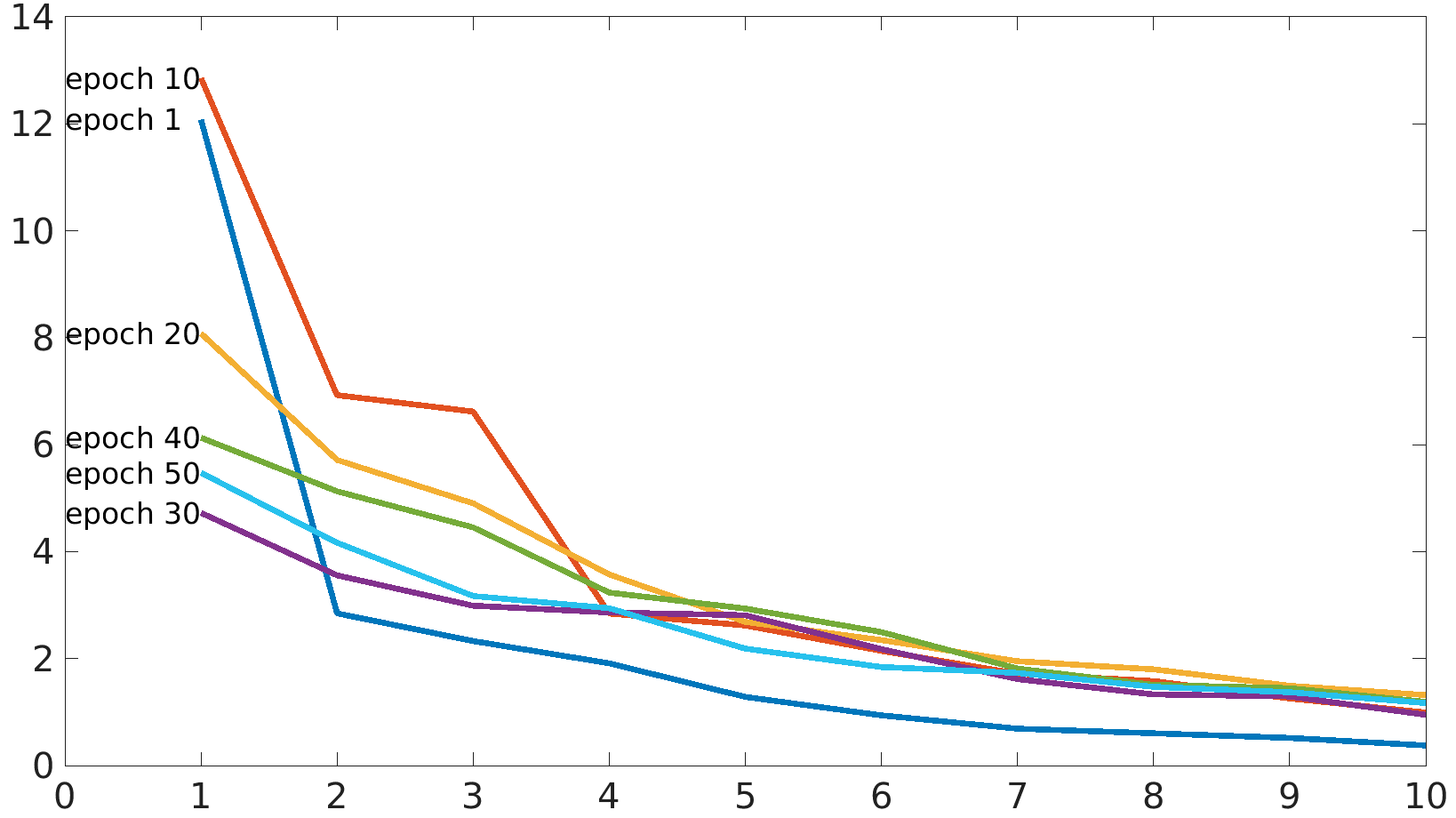
Figure 5: First 10 eigenvalues of distance matrices of 1024 random real data samples during training on CelebA.

4 Experiments

We conduct experiments on two tasks: unconditional image generation and single image super-resolution. To better understand the process of manifold matching, in both tasks we track various distances in batches during training. We represent distance between centroids of two sets as $d_{c}$, distance between $2$-diameters of two sets as $d_{g}$, and distance between paired SR-HR samples in super-resolution task as $d_{p}$, respectively. We also use Hausdorff distance as a measurement of distance between the two sets. Hausdorff distance is defined as ${\displaystyle d_{\mathrm{H}}(A,B)=\max\left\{\,\sup_{a\in A}\inf_{b\in B}d(a,b),\,\sup_{b\in B}\inf_{a\in A}d(a,b)\,\right\},\!}$, where $A$ and $B$ are two non-empty subsets of a metric space ($\mathcal{M},d$). Here we adopt Euclidean metric to calculate Hausdorff distance between two sets of Triplet network embedding, which is equivalent to measure Hausdorff distance between two sets of corresponding images in the image space under learned metric. All experiments are implemented under PyTorch framework using a Tesla V100 GPU.

4.1 Unconditional Image Generation

We use the matching criteria in Eqn 3.2 to validate the feasibility of the proposed framework. Note that no paired information or GAN loss is used for the task.

Implementation Details: We employed a ResNet data generator and a deep convolutional net metric generator with $\gamma=0.01$, $\lambda=1$, dimension of input latent vector $m=128$, and output embedding $n=10$ as our default setting. Adam optimizer with learning rate $1e-4$, $\beta_{1}=0$ and $\beta_{2}=0.9$ for data generator, and $\beta_{1}=0.5$ and $\beta_{2}=0.999$ for metric generator was used during training. Details of network architectures are provided in supplementary material.

Dataset and Evaluation Metrics: We implemented our method on CelebA [30] and LSUN bedroom [52] datasets. For training we used around 200K images in CelebA and 3M images in LSUN. All images were center-cropped and resized to $32\times 32$ or $64\times 64$. For each dataset we randomly generated 50K samples and used Fréchet Inception Distance (FID) [17] for quantitative evaluation. Smaller FID indicates better result.

Effect of Metric Learning on Distorting Real Data Manifold: During training we randomly choose 1024 real samples and detect its shape by looking at the eigenvalues of the corresponding (normalized) distance matrix. Particularly, we plot the first 10 largest eigenvalues which correspond to the size of the first 10 principle components of real samples. As shown in Fig. 5, the shape of the samples becomes more uniform with training going. This is an empirical evidence that $g_{w}$ distorts real data manifold to be uniformly curved. In this situation, matching centers and diameters should be enough for manifold matching.
Effects of Matching Different Geometric Descriptors: We study the effect of matching different geometric descriptors. Examples of generated $32\times 32$ samples on CelebA using different matching criteria are shown in Fig. 6. (i) Centroid matching learns some common shallow patterns from real data set; (ii) Matching $2$-diameters could capture more complicated intrinsic structures of the data manifold, while misalignment between the two sets can result in low-quality samples (e.g. image on the right side in the second last row); (iii) Combining the two descriptors together leads to more stable sample quality. We also visualize these manifold matching status for illustration purpose. We project output of $g_{w}$ to $2$-dim plane using UMAP [33], and display the projected points in Fig. 6 (a)(b)(c). (a) and (b) intuitively show two typical matching status if one only matches centroids or $2$-diameters between the two sets, respectively.

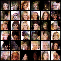
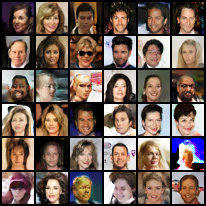
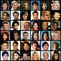
(i)	(ii)	(iii)
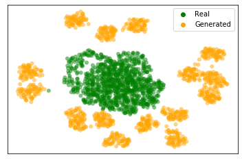
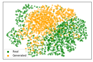
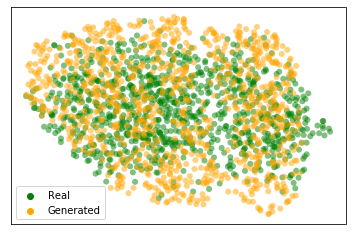
(a)	(b)	(c)

Figure 6: Randomly generated $32\times 32$ images on CelebA with different manifold matching criteria during training. (i) centroid only; (ii) $2$-diameter only; (iii) both centroid and $2$-diameter. (a)(b)(c) are corresponding UMAP plots of real (green) and generated (orange) samples with different manifold matching criteria. (a) centroid only; (b) $2$-diameter only; (c) both.

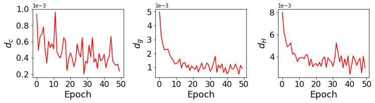
Figure 7: Distances versus training epochs in unconditional image generation task.

Table 2: Comparisons of results trained on different batch sizes.

Batch size	32	64	128	256	512	1024
Effective training	✓	✓	✓	✓	✓	✗
Time(s) / epoch	178	155	139	127	127	-

Effects of Batch Size: We further study the influence of batch size on training time and stability. Table 2 reports average training time per epoch on resized $32\times 32$ CelebA images. One can see batch size does not have a significant influence on average training time when matching $2$-diameters. In addition, we observe stable and efficient training sessions with different batch sizes. For batch size as large as $1024$, we did not observe satisfying sample quality in reasonable training time.

Table 3: Evaluation scores of different training settings in $\times 4$ SISR task. Demonstration of settings is displayed in Table 6. For each pair of settings with the same generator backbone, the one with better performance is highlighted.

	Set5				Set14				BSD100				Urban100
Setting	PSNR	SSIM	LPIPS	NIQE	PSNR	SSIM	LPIPS	NIQE	PSNR	SSIM	LPIPS	NIQE	PSNR	SSIM	LPIPS	NIQE
ResNet-GAN	29.03	0.8468	0.1885	7.2143	25.64	0.7420	0.2761	5.2654	25.74	0.7026	0.3160	5.3896	23.49	0.7273	0.2888	4.6504
ResNet-MvM	29.76	0.8606	0.1941	6.1478	26.12	0.7562	0.2724	5.3458	26.07	0.7150	0.3178	5.5508	24.06	0.7505	0.2774	4.7549
RDN-GAN	29.07	0.8442	0.1841	6.6459	25.38	0.7355	0.2729	5.3887	25.72	0.7029	0.3063	5.6734	23.11	0.7190	0.2876	4.6546
RDN-MvM	30.06	0.8658	0.1850	6.1283	26.31	0.7615	0.2641	5.2161	26.24	0.7210	0.3100	5.4127	24.44	0.7645	0.2566	4.5914
NSRNet-GAN	29.46	0.8544	0.1852	5.7818	25.93	0.7478	0.2666	5.1213	25.93	0.7094	0.3119	5.2069	23.70	0.7330	0.2832	5.1579
NSRNet-MvM	29.79	0.8641	0.1845	6.0846	26.17	0.7590	0.2655	5.3175	26.13	0.7188	0.3114	5.3794	24.19	0.7569	0.2621	4.5937

Quantitative Results: We track $d_{c},d_{g}$ and $d_{H}$ during training and display them in Fig. 7. With training going forward, the distances keep decreasing and gradually converge. The observation aligns with our manifold matching assumption even with no labelled information involved. For quantitative evaluation we present FID scores in Table 4. Here we also display results from some classic GAN frameworks using the same generator architecture. As shown in the table our method obtains competitive results.

Table 4: FID evaluation on $64\times 64$ experiments with a ResNet generator.

Method	CelebA	LSUN bedroom
WGAN [3]	37.1 (1.9)	73.3 (2.5)
WGAN-GP [15]	18.0 (0.7)	26.9 (1.1)
SNGAN [36]	21.7 (1.5)	31.3 (2.1)
SWGAN [50]	13.2 (0.7)	14.9 (1.0)
MvM	11.1 (0.1)	13.7 (0.3)

Examples of randomly generated samples are displayed in Fig. 8.

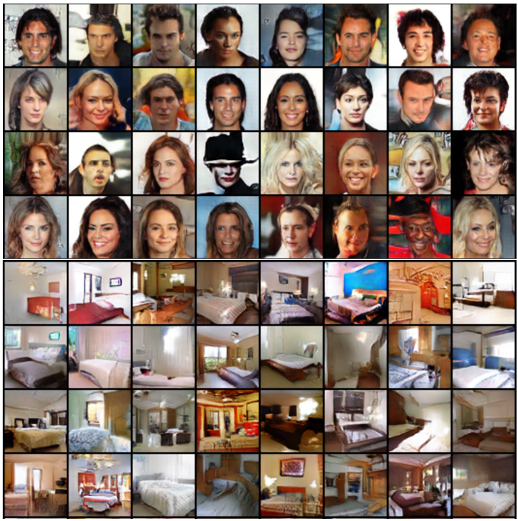
Figure 8: Randomly generated $64\times 64$ samples on CelebA and LSUN bedroom.

4.2 Single Image Super-Resolution

In a typical perception-based SR model [23, 46], the generator loss function is usually made up by three components: pixel-wise image loss, GAN loss and perceptual loss (or naturalness loss in [46]). Here we explore the use of our work with two different settings: (A) Our approach (MvM) serves as a substitute of GAN loss. In this case we use Eqn 3 as the total generator loss function without involving GAN loss; (B) MvM serves as a substitute of naturalness loss. In (B) MvM is used as a complement of GAN in perception-based models, where a GAN loss is added to Eqn 3 as the total generator loss.

Implementation Details: For setting (A), we compare MvM and GAN using three different generator backbones: ResNet [23], RDN [56] and NSRNet [46]. All experiments were conducted with the same training setup. For setting (B), we compare the effects of different perceptual components in perception-based models. We employed the ResNet architecture in [23] as the default generator backbone, and RaGAN [20] with weight $2e-3$ as GAN component for consistency. For both (A) and (B) we experimented on $\times 4$ SR task. We utilized Adam optimizer with learning rate $1e-4$, $\beta_{1}=0.9$, $\beta_{2}=0.999$ , metric learning direction guidance parameter $\gamma=1e-2$, weight of diameter matching term $\lambda=1$, dimension of Triplet network output embedding $n=32$, batch size $=32$ , $\lambda_{2}=\lambda_{3}=1e-3$, and trained for 100K iterations. Details of Triplet network architecture is presented in supplementary material.

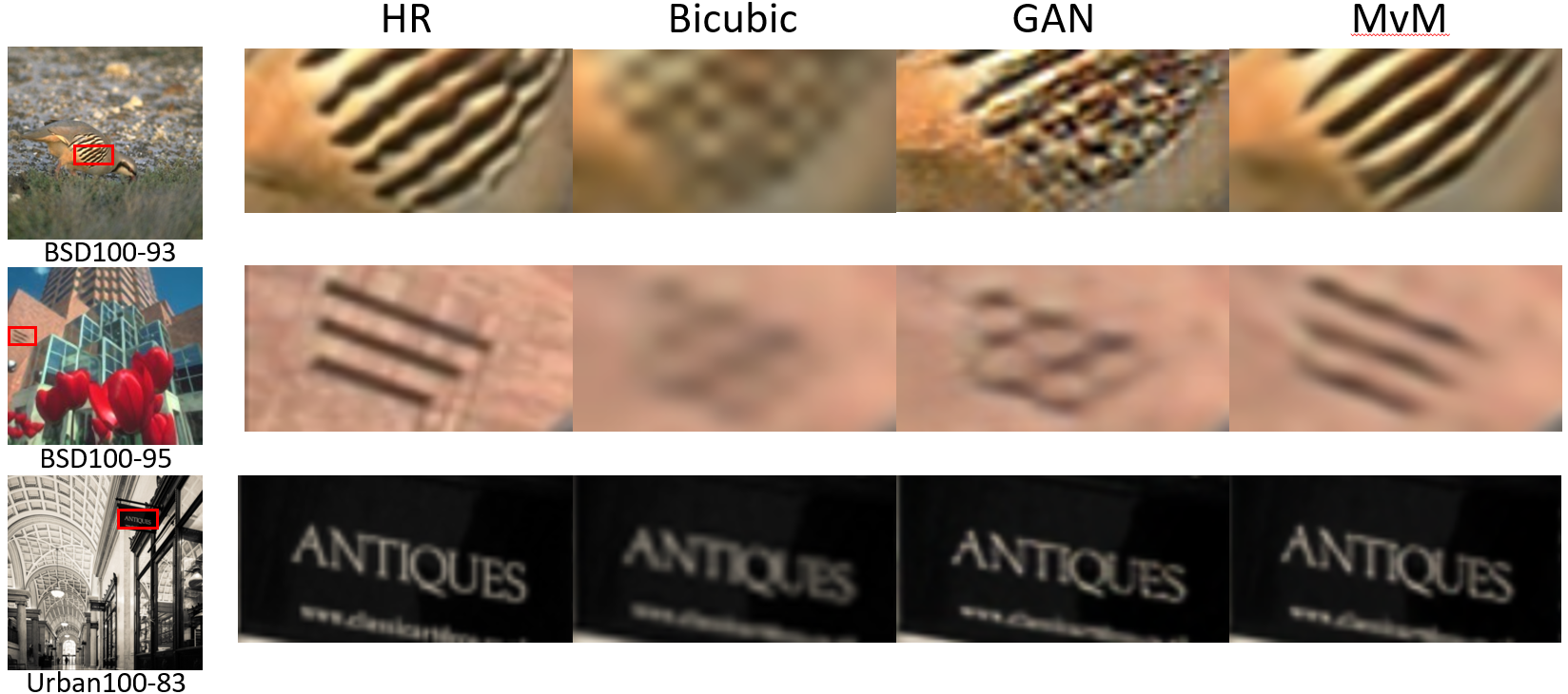
Figure 9: Generated $\times 4$ samples with GAN loss and MvM loss using the same generator backbone. (Zoom in for better view.)

Table 5: Evaluation scores of different training settings in $\times 4$ SISR task. Demonstration of settings is displayed in Table 6. The best performance is highlighted in red and second best in blue.

	Set5				Set14				BSD100				Urban100
Setting	PSNR	SSIM	LPIPS	NIQE	PSNR	SSIM	LPIPS	NIQE	PSNR	SSIM	LPIPS	NIQE	PSNR	SSIM	LPIPS	NIQE
A	28.42	0.8104	0.2977	7.3647	26.00	0.7027	0.3757	6.3393	25.96	0.6675	0.4637	6.2967	23.14	0.6577	0.4182	6.6429
B	29.66	0.8586	0.1401	6.6582	26.08	0.7542	0.2265	5.3638	26.05	0.7145	0.3257	5.5376	24.00	0.7464	0.2156	4.7883
C	29.30	0.8445	0.1324	6.6590	25.81	0.7394	0.2132	5.5318	25.81	0.7010	0.3006	5.8399	23.83	0.7346	0.2047	4.6377
D	29.75	0.8593	0.1357	6.5475	26.11	0.7542	0.2193	5.3559	26.06	0.7145	0.3160	5.6108	24.15	0.7506	0.2028	4.7447
E	29.63	0.8547	0.1227	6.2838	26.07	0.7512	0.2051	5.0657	26.05	0.7119	0.2957	5.2257	24.12	0.7484	0.1862	4.2814
F	29.70	0.8603	0.1409	6.2673	26.06	0.7556	0.2239	5.3777	26.05	0.7146	0.3218	5.6095	23.98	0.7477	0.2126	4.7880
G	29.87	0.8615	0.1281	5.8904	26.17	0.7564	0.2048	4.9612	26.10	0.7134	0.2930	4.9864	24.25	0.7567	0.1866	4.3432

Datasets and Evaluation Metrics: We used 800 HR images in DIV2K [2] dataset as training set, and four benchmark datasets: Set5 [5], Set14 [53], BSD100 [32] and Urban100 [19] for testing. HR images were downsampled by bicubic interpolation to get $48\times 48$ LR input patches. We evaluated results using Structure Similarity (SSIM) [49], PSNR as distortion-oriented evaluation metrics, and Naturalness Image Quality Evaluator (NIQE) [35], Learned Perceptual Image Patch Similarity (LPIPS) [54] as perception-oriented evaluation metrics. Lower NIQE and LPIPS scores indicate higher perceptual quality.

Table 6: Training settings for GAN-based SISR methods with fixed generator architecture and GAN component.

Setting	Method	Perceptual component	Pretrained
A	Bicubic	-	-
B	GAN-ResNet	-	-
C	SRGAN	VGG16-Pooling5	Yes
D	EnhanceNet	VGG19-Pooling2,5	Yes
E	ESRGAN	VGG19-Conv5-4	Yes
F	NatSR	NMD	Yes
G(ours)	MvM	MM	No

Results: We record $d_{p},d_{c},d_{g}$, and Hausdorff distance $d_{H}$ during training and display them in Fig.10. One can see all distances keeps decreasing with training going forward, which is aligned with our basic assumption that the two sets of points keep getting close to each other. Note that the spike effect is common for Adam optimizer when feeding some abnormal random batch of training data.

Figure 10: Various distances versus training epochs in super-resolution experiment with our method. Distances are displayed every 40 epochs (1000 iterations).

(A) MvM As A Substitute of GAN Loss: We display comparison of evaluation results between GAN and MvM in Table 3. Under different backbones, MvM performs better than GAN in similarity-based metrics in all cases. It also obtains better scores in perception-based metrics in majority of the cases. Examples of generated samples using the same generator backbone are displayed in Fig. 9. We see MvM resulted in samples with more natural textures.

(B) MvM As A Substitute of Naturalness Loss: We display a few different setups in Table 6. Final results with both distortion-based and perception-based evaluation scores on benchmark datasets are presented in Table 5, where GAN-ResNet represents SRGAN without VGG component in loss function. With the same common setup, MvM obtained better results in most of the cases for both types of metrics. Examples of generated samples from various settings are shown in Fig. 11. As we see MvM generates samples with more natural textures and less artifacts under the same setup.

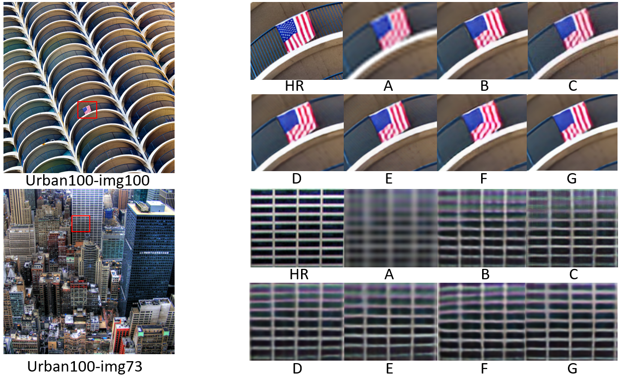
Figure 11: Comparison of generated samples from different settings. All settings were trained with the same ResNet generator backbone and GAN components. (Zoom in for better view.)

We notice that although both GAN and MvM utilize adversarial learning for training, the two approaches behave differently in super-resolution task. GAN tends to generate more details but with artifacts, while MvM tends to generate more natural textures in images. The two approaches do not conflict with each other. Instead, one serves as a complement for the other to result in better sample quality.

5 Discussion and Conclusion

In this paper, we have proposed a manifold matching approach for generative modeling, which matches geometric descriptors of real and generated data sets using learned distance metrics. Experiments on two tasks validated its feasibility and effectiveness. Moreover, the proposed framework is robust and flexible in that each network has its own designated objective. Despite that our method has led to some promising results, there is yet much room for improvements. For example, the currently used geometric descriptors may not fully recover the information of the underlying manifolds, thus matching towards other descriptors could potentially benefit the learning process. As to metric learning, in our paper we employ the method in [37] fed with random samples to learn a metric, while in practice one could investigate ways for better approximation of metrics, such as utilizing sampling methods or other metric learning methods. In addition, although empirical evidences and intuitions agree with the current metric measure space setting, further theoretical analysis using optimal transport is worth exploring. In the last few years we have witnessed great success of probability-based generative modeling approaches, and we believe joining geometry with statistics would lead to stronger expression ability for generative models, which is a promising direction for researchers to explore.

6 Acknowledgment

MD and HH would like to thank the four anonymous reviewers especially Reviewer 1 and Reviewer 4 for their valuable comments. HH acknowledges partial support by NSF grant DMS-1854683.

7 Proofs of Properties

Given any space $X$ associated with a probability measure $\mu$ s.t. $\operatorname{supp}[\mu]=X$ and $p\geq 1$, then for any function $f:X\rightarrow\mathbb{R}$ we denote its $L^{p}$ norm as

$$\|f\|_{p}:=\left(\int_{X}|f(x)|^{p}d\mu(x)\right)^{1/p}.$$

Then we have the following properties:

Lemma 7.1.

Denote $\|f\|_{\infty}:=\sup_{x\in X}f(x)$, then

1. If $p\leq q$, then $\|f\|_{p}\leq\|f\|_{q}$;

2. $\lim_{p\to\infty}\|f\|_{p}=\|f\|_{\infty}$.

Proof.

Let $r=q/p$ and $s$ be such that $1/r+1/s=1$. Let $a(x)=|f(x)|^{p}$ and $b(x)\equiv 1$, then by Holder’s inequality, we have

$$\|ab\|_{1}\leq\|a\|_{r}\|b\|_{s}$$

or

$$\int_{x\in X}|f(x)|^{p}d\mu(x)\leq\left(\int_{x\in X}|f(x)|^{p\cdot\frac{q}{p}}d\mu(x)\right)^{p/q}.$$

Now taking the $p$-th root on both sides we obtain $\|f\|_{p}\leq\|f\|_{q}$.

It is easy to see $\|f\|_{p}\leq\|f\|_{\infty}$ for any $p>1$. Now we choose $\forall\epsilon>0$ with $\epsilon<\|f\|_{\infty}$ and let $X_{\epsilon}:=\{x\in X|f(x)\geq\|f\|_{\infty}-\epsilon\}$, then

$$\left(\int_{x\in X}|f(x)|^{p}d\mu(x)\right)^{1/p}$$

$$\geq \left(\int_{X_{\epsilon}}(\|f\|_{\infty}-\epsilon)^{p}d\mu(x)\right)^{1/p}$$

$$= (\|f\|_{\infty}-\epsilon)\mu(X_{\epsilon})^{1/p}$$

When $p\to\infty$ we have $\lim_{p\to\infty}\|f\|_{p}\geq\|f\|_{\infty}-\epsilon$. Since $\epsilon$ is arbitrary we have $\lim_{p\to\infty}\|f\|_{p}\geq\|f\|_{\infty}$. ∎

8 Properties of Geometric Descriptors

Given metric measure space $\mathcal{X}=(X,d,\mu)$, intuitively, the Fréchet mean set $\sigma(\mathcal{X})$ represents the center of $\mathcal{X}$ with respect to metric $d$. Particularly,

Lemma 8.1.

The Fréchet mean of measure $\mu$ with respect to $d_{E}$ coincides with the mean $\overline{\mu}:=\int_{\mathbb{R}^{D}}yd\mu(y)$.

Proof.

Suppose that elements in $\mathbb{R}^{D}$ are represented as column vectors. Then $\sigma(\mathbb{R}^{D},d,\mu)$ equals the set of minimizers of

$$F(x)=\int_{\mathbb{R}^{D}}(y-x)^{T}(y-x)d\mu(y).$$

Since $\frac{\partial F}{\partial x}=-2\int_{\mathbb{R}^{D}}yd\mu(y)+2x$, let $\frac{\partial F}{\partial x}=0$ we have single minimizer of $F(x)$ to be $\int_{\mathbb{R}^{D}}yd\mu(y)=\overline{\mu}$. ∎

When the underlying metric $d$ is not the Euclidean metric, the Fréchet mean provides a better option of centroid.

Let $x_{1},x_{2},\cdots,x_{k},\cdots$ be a sequence of independent identically distributed points sampled from $\mu$. Let $\mu_{k}=\frac{1}{k}\Sigma_{i=1}^{k}\delta_{x_{i}}$ denote the empirical measure. We can estimate the Fréchet mean of $(X,d,\mu)$ by a set of random samples:

Proposition 8.2.

$\sigma(\mathcal{X})=\lim_{k\to\infty}\sigma(X,d,\mu_{k}).$

Proof.

Since the empirical measure $\mu_{k}$ weakly converges to $\mu$, the result following by the definition of weak convergence. ∎

The following lemma explains its geometric meaning of $p$-diameters:

Lemma 8.3.

For any metric measure space $\mathcal{X}:=(X,d,\mu)$ with $\operatorname{supp}[\mu]=X$,

1. $\operatorname{diam}_{p}(\mathcal{X})\leq\operatorname{diam}_{q}(\mathcal{X})$ for any $p\leq q$;

2. $\lim_{p\to\infty}\operatorname{diam}_{p}(\mathcal{X})=\sup\limits_{x,x^{\prime}\in X}d(x,x^{\prime})$.

Proof.

It follows directly from Lemma 7.1 ∎

Similarly, we can estimate the $p$-diameter of a metric measure space $\mathcal{X}:=(X,d,\mu)$ by a set of random samples:

Proposition 8.4.

$$\operatorname{diam}_{p}(\mathcal{X})=\lim_{k\to\infty}\operatorname{diam}_{p}(X,d,\mu_{k}).$$

Proof.

Since the empirical measure $\mu_{k}$ weakly converges to $\mu$, the result following by the definition of weak convergence. ∎

Proposition 8.5.

Given a metric measure space $\mathcal{X}:=(X,d,\mu)$ and map $g:X\rightarrow\mathbb{R}^{n}$. If $d=g^{\ast}d_{E}$, then

$$\sigma(\mathcal{X})=g^{-1}(\overline{g_{\ast}\mu}).$$

Proof.

By definition, $\sigma(\mathcal{X})$ is the set of minimizers of function

$$F(x): =\int_{X}(g^{\ast}d_{E})^{2}(x,y)d\mu(y)$$

$$=\int_{X}d^{2}_{E}(g(x),g(y))d\mu(y)$$

$$=\int_{\mathbb{R}^{n}}d^{2}_{E}(g(x),z)d(g_{\ast}\mu)(z).$$

It is easy to see that $x_{0}$ is a minimizer of $F(x)$ iff. $g(x_{0})$ is a minimizer of $G(w):=\int_{\mathbb{R}^{n}}d^{2}_{E}(w,z)d(g_{\ast}\mu)(z)$. By Lemma 3.4, $\overline{g_{\ast}\mu}=\operatorname{argmin}G(w)$, hence we have $\sigma(\mathcal{X})=\operatorname{argmin}F(x)=g^{-1}(\overline{g_{\ast}\mu})$. ∎

Proof of Proposition 3.10.

It follows directly from Proposition 8.5 ∎

9 Network Architectures

For unconditional image generation task, we used a ResNet data generator and a deep convolutional net metric generator:

$f_{\theta}$: convt(128) $\rightarrow$ upres(128) $\rightarrow$ upres(128) $\rightarrow$ upres(128) $\rightarrow$ upres(128) $\rightarrow$ bn $\rightarrow$ conv(128) $\rightarrow$ sig;

$g_{w}$: conv(32) $\rightarrow$ leaky-relu(0.2) $\rightarrow$ conv(64) $\rightarrow$ leaky-relu(0.2) $\rightarrow$ conv(128) $\rightarrow$ leaky-relu(0.2) $\rightarrow$ conv(256) $\rightarrow$ leaky-relu(0.2) $\rightarrow$ conv(512) $\rightarrow$ leaky-relu(0.2) $\rightarrow$ maxpool $\rightarrow$ dense(10).

For super-resolution task, the architecture of Triplet embedding network is presented as below:

$g_{w}$: (conv(x$\rightarrow$2x, $x_{0}$=32) $\rightarrow$ prelu $\rightarrow$ maxpool) * 7 $\rightarrow$ dense(256) $\rightarrow$ prelu $\rightarrow$ dense(256) $\rightarrow$ prelu $\rightarrow$ dense(32),

where conv, convt, upres, bn, relu, leaky-relu, prelu, maxpool, dense and sig refer to nn.Conv2d, nn.ConvTranspose2d, up-ResidualBlock, nn.BatchNorm2d, nn.ReLU, nn.LeakyReLU, nn.PReLu, nn.MaxPool2d, nn.Linear and nn.Sigmoid layers in Pytorch framework respectively.

10 More Evaluation Details

Perception-Based Evaluations in SISR: we adopted the function $niqe$ in Matlab for computing NIQE scores, and python package $lpips$ for computing LPIPS.

FID Evaluation: we used 50000 randomly generated samples comparing against 50000 random samples from real data sets for testing. Features were extracted from the pool3 layer of a pre-trained Inception network. FID was computed over 10 bootstrap resamplings.

References

- [1] Charu C. Aggarwal, Alexander Hinneburg, and Daniel A. Keim. On the surprising behavior of distance metrics in high dimensional spaces. In Proceedings of the 8th International Conference on Database Theory. Springer-Verlag, 2001.
- [2] Eirikur Agustsson and Radu Timofte. Ntire 2017 challenge on single image super-resolution: Dataset and study. In The IEEE Conference on Computer Vision and Pattern Recognition (CVPR) Workshops, July 2017.
- [3] Martin Arjovsky, Soumith Chintala, and Léon Bottou. Wasserstein generative adversarial networks. In Proceedings of the 34th International Conference on Machine Learning, volume 70, pages 214–223, 2017.
- [4] Marc Arnaudon, Frédéric Barbaresco, and Le Yang. Medians and means in riemannian geometry: existence, uniqueness and computation. In Matrix Information Geometry, pages 169–197. Springer, 2013.
- [5] Marco Bevilacqua, Aline Roumy, Christine Guillemot, and Marie line Alberi Morel. Low-complexity single-image super-resolution based on nonnegative neighbor embedding. In Proceedings of the British Machine Vision Conference, pages 135.1–135.10. BMVA Press, 2012.
- [6] Goutam Bhat, Martin Danelljan, Luc Van Gool, and Radu Timofte. Deep burst super-resolution. In Proceedings of the IEEE/CVF Conference on Computer Vision and Pattern Recognition (CVPR), pages 9209–9218, June 2021.
- [7] Rabi Bhattacharya and Vic Patrangenaru. Large sample theory of intrinsic and extrinsic sample means on manifolds. The Annals of Statistics, 31(1):1–29, 2003.
- [8] Jianrui Cai, Hui Zeng, Hongwei Yong, Zisheng Cao, and Lei Zhang. Toward real-world single image super-resolution: A new benchmark and a new model. In Proceedings of the IEEE/CVF International Conference on Computer Vision (ICCV), October 2019.
- [9] Ishan Deshpande, Yuan-Ting Hu, Ruoyu Sun, Ayis Pyrros, Nasir Siddiqui, Sanmi Koyejo, Zhizhen Zhao, David Forsyth, and Alexander G. Schwing. Max-sliced wasserstein distance and its use for gans. In Proceedings of the IEEE/CVF Conference on Computer Vision and Pattern Recognition (CVPR), June 2019.
- [10] Zheng Ding, Yifan Xu, Weijian Xu, Gaurav Parmar, Yang Yang, Max Welling, and Zhuowen Tu. Guided variational autoencoder for disentanglement learning. In Proceedings of the IEEE/CVF Conference on Computer Vision and Pattern Recognition (CVPR), June 2020.
- [11] Yueqi Duan, Wenzhao Zheng, Xudong Lin, Jiwen Lu, and Jie Zhou. Deep adversarial metric learning. In Proceedings of the IEEE Conference on Computer Vision and Pattern Recognition (CVPR), June 2018.
- [12] Aude Genevay, Gabriel Peyre, and Marco Cuturi. Learning generative models with sinkhorn divergences. In Proceedings of the Twenty-First International Conference on Artificial Intelligence and Statistics, volume 84 of Proceedings of Machine Learning Research, pages 1608–1617, 2018.
- [13] Ian Goodfellow, Jean Pouget-Abadie, Mehdi Mirza, Bing Xu, David Warde-Farley, Sherjil Ozair, Aaron Courville, and Yoshua Bengio. Generative adversarial nets. In Advances in neural information processing systems, pages 2672–2680, 2014.
- [14] Karsten Grove and Hermann Karcher. How to conjugatec -close group actions. Mathematische Zeitschrift, 132(1):11–20, 1973.
- [15] Ishaan Gulrajani, Faruk Ahmed, Martin Arjovsky, Vincent Dumoulin, and Aaron C Courville. Improved training of wasserstein gans. In I. Guyon, U. V. Luxburg, S. Bengio, H. Wallach, R. Fergus, S. Vishwanathan, and R. Garnett, editors, Advances in Neural Information Processing Systems, volume 30, 2017.
- [16] Yong Guo, Jian Chen, Jingdong Wang, Qi Chen, Jiezhang Cao, Zeshuai Deng, Yanwu Xu, and Mingkui Tan. Closed-loop matters: Dual regression networks for single image super-resolution. In IEEE/CVF Conference on Computer Vision and Pattern Recognition (CVPR), June 2020.
- [17] Martin Heusel, Hubert Ramsauer, Thomas Unterthiner, Bernhard Nessler, and Sepp Hochreiter. Gans trained by a two time-scale update rule converge to a local nash equilibrium. arXiv preprint arXiv:1706.08500, 2017.
- [18] Elad Hoffer and Nir Ailon. Deep metric learning using triplet network. In International Workshop on Similarity-Based Pattern Recognition, pages 84–92. Springer, 2015.
- [19] Jia-Bin Huang, Abhishek Singh, and Narendra Ahuja. Single image super-resolution from transformed self-exemplars. In Proceedings of the IEEE Conference on Computer Vision and Pattern Recognition (CVPR), June 2015.
- [20] Alexia Jolicoeur-Martineau. The relativistic discriminator: a key element missing from standard GAN. CoRR, abs/1807.00734, 2018.
- [21] Diederik P. Kingma and Max Welling. Auto-Encoding Variational Bayes. In 2nd International Conference on Learning Representations, ICLR 2014, Banff, AB, Canada, April 14-16, 2014, Conference Track Proceedings, 2014.
- [22] Yann LeCun, Sumit Chopra, Raia Hadsell, Fu Jie Huang, and et al. A tutorial on energy-based learning. In PREDICTING STRUCTURED DATA. MIT Press, 2006.
- [23] Christian Ledig, Lucas Theis, Ferenc Huszár, Jose Caballero, Andrew Cunningham, Alejandro Acosta, Andrew Aitken, Alykhan Tejani, Johannes Totz, Zehan Wang, et al. Photo-realistic single image super-resolution using a generative adversarial network. In Proceedings of the IEEE conference on computer vision and pattern recognition, pages 4681–4690, 2017.
- [24] Chen-Yu Lee, Tanmay Batra, Mohammad Haris Baig, and Daniel Ulbricht. Sliced wasserstein discrepancy for unsupervised domain adaptation. In Proceedings of the IEEE/CVF Conference on Computer Vision and Pattern Recognition (CVPR), June 2019.
- [25] Na Lei, Kehua Su, Li Cui, Shing-Tung Yau, and David Xianfeng Gu. A geometric view of optimal transportation and generative model, 2017.
- [26] Chun-Liang Li, Wei-Cheng Chang, Yu Cheng, Yiming Yang, and Barnabás Póczos. Mmd gan: Towards deeper understanding of moment matching network. In Advances in Neural Information Processing Systems, pages 2203–2213, 2017.
- [27] Bee Lim, Sanghyun Son, Heewon Kim, Seungjun Nah, and Kyoung Mu Lee. Enhanced deep residual networks for single image super-resolution. In Proceedings of the IEEE Conference on Computer Vision and Pattern Recognition (CVPR) Workshops, July 2017.
- [28] Jae Hyun Lim and Jong Chul Ye. Geometric gan, 2017.
- [29] Jie Liu, Wenjie Zhang, Yuting Tang, Jie Tang, and Gangshan Wu. Residual feature aggregation network for image super-resolution. In IEEE/CVF Conference on Computer Vision and Pattern Recognition (CVPR), June 2020.
- [30] Ziwei Liu, Ping Luo, Xiaogang Wang, and Xiaoou Tang. Deep learning face attributes in the wild. In Proceedings of International Conference on Computer Vision (ICCV), December 2015.
- [31] Cheng Ma, Yongming Rao, Yean Cheng, Ce Chen, Jiwen Lu, and Jie Zhou. Structure-preserving super resolution with gradient guidance. In IEEE/CVF Conference on Computer Vision and Pattern Recognition (CVPR), June 2020.
- [32] David Martin, Charless Fowlkes, Doron Tal, and Jitendra Malik. A database of human segmented natural images and its application to evaluating segmentation algorithms and measuring ecological statistics. In Proceedings Eighth IEEE International Conference on Computer Vision. ICCV 2001, volume 2, pages 416–423. IEEE, 2001.
- [33] Leland McInnes, John Healy, Nathaniel Saul, and Lukas Großberger. Umap: Uniform manifold approximation and projection. Journal of Open Source Software, 3(29):861, 2018.
- [34] Facundo Mémoli. Gromov–wasserstein distances and the metric approach to object matching. Foundations of computational mathematics, 11(4):417–487, 2011.
- [35] Anish Mittal, Rajiv Soundararajan, and Alan C Bovik. Making a “completely blind” image quality analyzer. IEEE Signal processing letters, 20(3):209–212, 2012.
- [36] Takeru Miyato, Toshiki Kataoka, Masanori Koyama, and Yuichi Yoshida. Spectral normalization for generative adversarial networks. In International Conference on Learning Representations, 2018.
- [37] Deen Dayal Mohan, Nishant Sankaran, Dennis Fedorishin, Srirangaraj Setlur, and Venu Govindaraju. Moving in the right direction: A regularization for deep metric learning. In Proceedings of the IEEE/CVF Conference on Computer Vision and Pattern Recognition (CVPR), June 2020.
- [38] Noseong Park, Ankesh Anand, Joel Ruben Antony Moniz, Kookjin Lee, Jaegul Choo, David Keetae Park, Tanmoy Chakraborty, Hongkyu Park, and Youngmin Kim. Mmgan: Manifold-matching generative adversarial networks. In 2018 24th International Conference on Pattern Recognition (ICPR), pages 1343–1348. IEEE, 2018.
- [39] Carey E. Priebe, David J. Marchette, Zhiliang Ma Jhu, and Sancar Adali Jhu. Manifold matching: Joint optimization of fidelity and commensurability, 2010.
- [40] Yajun Qiu, Ruxin Wang, Dapeng Tao, and Jun Cheng. Embedded block residual network: A recursive restoration model for single-image super-resolution. In Proceedings of the IEEE/CVF International Conference on Computer Vision (ICCV), October 2019.
- [41] Kanishka Rao, Chris Harris, Alex Irpan, Sergey Levine, Julian Ibarz, and Mohi Khansari. Rl-cyclegan: Reinforcement learning aware simulation-to-real. In Proceedings of the IEEE/CVF Conference on Computer Vision and Pattern Recognition (CVPR), June 2020.
- [42] Michal Rolinek, Dominik Zietlow, and Georg Martius. Variational autoencoders pursue pca directions (by accident). In Proceedings of the IEEE/CVF Conference on Computer Vision and Pattern Recognition (CVPR), June 2019.
- [43] Mehdi SM Sajjadi, Bernhard Scholkopf, and Michael Hirsch. Enhancenet: Single image super-resolution through automated texture synthesis. In Proceedings of the IEEE International Conference on Computer Vision, pages 4491–4500, 2017.
- [44] Hang Shao, Abhishek Kumar, and P. Thomas Fletcher. The riemannian geometry of deep generative models. In Proceedings of the IEEE Conference on Computer Vision and Pattern Recognition (CVPR) Workshops, June 2018.
- [45] Cencheng Shen, J. Vogelstein, and C. Priebe. Manifold matching using shortest-path distance and joint neighborhood selection. Pattern Recognit. Lett., 92:41–48, 2017.
- [46] Jae Woong Soh, Gu Yong Park, Junho Jo, and Nam Ik Cho. Natural and realistic single image super-resolution with explicit natural manifold discrimination. In The IEEE Conference on Computer Vision and Pattern Recognition (CVPR), June 2019.
- [47] Cédric Villani. Optimal transport: old and new, volume 338. Springer Science & Business Media, 2008.
- [48] Xintao Wang, Ke Yu, Shixiang Wu, Jinjin Gu, Yihao Liu, Chao Dong, Yu Qiao, and Chen Change Loy. Esrgan: Enhanced super-resolution generative adversarial networks. In The European Conference on Computer Vision Workshops (ECCVW), September 2018.
- [49] Zhou Wang, Alan C. Bovik, Hamid R. Sheikh, and Eero P. Simoncelli. Image quality assessment: From error visibility to structural similarity. IEEE TRANSACTIONS ON IMAGE PROCESSING, 13(4):600–612, 2004.
- [50] Jiqing Wu, Zhiwu Huang, Dinesh Acharya, Wen Li, Janine Thoma, Danda Pani Paudel, and Luc Van Gool. Sliced wasserstein generative models. In Proceedings of the IEEE/CVF Conference on Computer Vision and Pattern Recognition (CVPR), June 2019.
- [51] Eric P Xing, Michael I Jordan, Stuart J Russell, and Andrew Y Ng. Distance metric learning with application to clustering with side-information. In Advances in neural information processing systems, pages 521–528, 2003.
- [52] Fisher Yu, Yinda Zhang, Shuran Song, Ari Seff, and Jianxiong Xiao. Lsun: Construction of a large-scale image dataset using deep learning with humans in the loop. CoRR, abs/1506.03365, 2015.
- [53] Roman Zeyde, Michael Elad, and Matan Protter. On single image scale-up using sparse-representations,” curves and surfaces, 2012.
- [54] Richard Zhang, Phillip Isola, Alexei A Efros, Eli Shechtman, and Oliver Wang. The unreasonable effectiveness of deep features as a perceptual metric. In Proceedings of the IEEE conference on computer vision and pattern recognition, pages 586–595, 2018.
- [55] Yuxuan Zhang, Wenzheng Chen, Huan Ling, Jun Gao, Yinan Zhang, Antonio Torralba, and Sanja Fidler. Image {gan}s meet differentiable rendering for inverse graphics and interpretable 3d neural rendering. In International Conference on Learning Representations, 2021.
- [56] Yulun Zhang, Yapeng Tian, Yu Kong, Bineng Zhong, and Yun Fu. Residual dense network for image super-resolution. In Proceedings of the IEEE conference on computer vision and pattern recognition, pages 2472–2481, 2018.