A Compressive Multi-Kernel Method for Privacy-Preserving Machine Learning

Abstract

As the analytic tools become more powerful, and more data are generated on a daily basis, the issue of data privacy arises. This leads to the study of the design of privacy-preserving machine learning algorithms. Given two objectives, namely, utility maximization and privacy-loss minimization, this work is based on two previously non-intersecting regimes – Compressive Privacy and multi-kernel method. Compressive Privacy is a privacy framework that employs utility-preserving lossy-encoding scheme to protect the privacy of the data, while multi-kernel method is a kernel-based machine learning regime that explores the idea of using multiple kernels for building better predictors. In relation to the neural-network architecture, multi-kernel method can be described as a two-hidden-layered network with its width proportional to the number of kernels.

The compressive multi-kernel method proposed consists of two stages – the compression stage and the multi-kernel stage. The compression stage follows the Compressive Privacy paradigm to provide the desired privacy protection. Each kernel matrix is compressed with a lossy projection matrix derived from the Discriminant Component Analysis (DCA). The multi-kernel stage uses the signal-to-noise ratio (SNR) score of each kernel to non-uniformly combine multiple compressive kernels.

The proposed method is evaluated on two mobile-sensing datasets – MHEALTH and HAR – where activity recognition is defined as utility and person identification is defined as privacy. The results show that the compression regime is successful in privacy preservation as the privacy classification accuracies are almost at the random-guess level in all experiments. On the other hand, the novel SNR-based multi-kernel shows utility classification accuracy improvement upon the state-of-the-art in both datasets. These results indicate a promising direction for research in privacy-preserving machine learning.

I Introduction

Kernel-based machine learning has been a successful paradigm in various data analytic applications [1, 2, 3, 4]. Traditionally, a single kernel is chosen for each system by the user’s expertise and experience. More recent works have investigated the possibility of using more than one kernel in a system [1, 5, 6, 7, 8, 9, 10]. The results from these recent works suggest that this multi-kernel method is attractive in improving the utility of the learning system. From the perspective of neural network architecture, the multi-kernel method can be viewed as a two-hidden-layered network with the first hidden layer corresponds to the kernel feature vector mapping, and the second hidden layer corresponds to the combination of multiple kernel feature vectors. However, the learning is only required on the second hidden layer, as the first first hidden layer is defined by the kernels. An illustration of the first hidden layer can be found in [1]. Importantly, the width of the first hidden layer depends on the number kernels, so higher number of kernels yields wider networks.

Concurrently, as the data analytical tools become more powerful and more data are being collected on the daily basis, the concern of data privacy arises. This is evident from several data leakage incidents that have been reported [11]. Moreover, the leakage can even occur when the data are intentionally released with anonymity [12, 13, 14, 15]. This shows that security and anonymity may not be sufficient to provide privacy protection. To this end, a new regime of data privacy preservation has been proposed to protect privacy at the user end before the data are shared to the public space. This regime of Compressive Privacy [16, 17] aims at modifying the data in a lossy fashion in order to limit the amount of information on the data released.

Naturally, using multiple kernels in a machine learning system increases the amount of information involved in the learning process. This, therefore, may provide a challenge in terms of privacy. Although several works have been carried out on multi-kernel machine learning, they almost exclusively focus on improving utility of the system. However, in the current era when privacy concern has become more prevalent, in order for a multi-kernel machine learning system to be applicable in the real world, privacy preservation should be incorporated into the design of the system.

In this work, Compressive Privacy is applied to multi-kernel machine learning to propose a compressive multi-kernel learning system. The system consists of two steps – the compression step and the multi-kernel step. In the compression step, each kernel is rank-reduced to produce a lossy kernel matrix, while in the multi-kernel step, multiple lossy kernel matrices are combined to generate the final multi-kernel matrix to be used in the learning process. The primary focus of this work is on the classification problem and two classification problems are defined – one for utility and one for privacy. The design goal is to yield high utility accuracy, while allowing low privacy accuracy.

The compression step utilizes a powerful dimensionality reduction framework called Discriminant Component Analysis (DCA) [1, 18, 19]. DCA allows the dimensionality reduction to be targeted to a specified goal, namely, utility classification. More importantly, given $L_{u}$ classes of utility classification, DCA only requires $L_{u}-1$ dimensions to reach the maximum discriminant power, permitting high compression when $L_{u}$ is much less than the original dimension of the data. The multi-kernel step, meanwhile, employs the non-negative linear combination of kernels, using a novel non-uniform weighting method based on the signal-to-noise ratio (SNR) score of each kernel, as inspired by the inter-class separability metric presented in [16].

The proposed method is evaluated on two datasets – MHEALTH [20, 21], and HAR [22]. Both datasets are related to mobile sensing, of which application is apparent in the current world of ubiquitous smartphones. For both datasets, the classification of human activity is defined as utility, whereas identification of the subject the features are generated from is defined as privacy. Two experiments are performed on each dataset. The first experiment uses multiple radial basis function (RBF) kernels with different gamma values, while the second uses different types of kernels.

The experimental results show that the proposed compressive SNR-based multi-kernel learning system can improve the utility accuracy when compared to the compressive single kernel, the compressive uniform multi-kernel, and the compressive alignment-based multi-kernel learning systems in all experiments. On the other hand, the privacy accuracy is reduced to almost random guess in all experiments. The compressive multi-kernel learning method, therefore, presents a promising framework for privacy-preserving machine learning applications.

II Prior Works

II-A Compressive Privacy

Compressive Privacy [16, 17] is a privacy paradigm of which the main principle is based on lossy encoding. In Compressive Privacy, the utility and privacy are known to the system designer. Consequently, the lossy encoding scheme can be designed such that it is information-preserving with respect to the utility, but information-lossy with respect to the privacy.

Another important principle of Compressive Privacy is that the data privacy protection should be managed by the data owners. Therefore, Compressive Privacy defines two different spheres in the world of data privacy – the private sphere and the public sphere. The private sphere is where the data owners generate and manage the lossy encoding of the data, whereas the public sphere is where the data are available to the authorized users and, at the same time, to the possible adversary. Therefore, in Compressive Privacy, data need to be transformed in a privacy-lossy, utility-preserving way in the private sphere before being transferred to the public sphere.

II-B Multi-Kernel Method

The study of the multi-kernel method arises from the traditional need to hand-design a kernel for an application, and the idea that combining multiple kernels should be more powerful than a single kernel. This has been a problem of interest in the research community both in theoretical, and application viewpoints. Several works have investigated different ways of formulating kernel combination including using semidefinite programming [7], semi-infinite programming [23], convex combination [24, 25, 26], non-stationary combination [27], and sparse combination [28]. At the same time, several applications of the multi-kernel method have been proposed such as in image analysis [29, 30], neuroimaging [31], signal processing [32], and stock market prediction [33].

Arguably, the most common kernel combination method is the non-negative linear combination of kernels, which can be viewed as a convex combination of a finite set of kernels. This multi-kernel is, thus, in the form,

$$\mathbf{K}_{\mu}=\sum_{l=1}^{P}\mu_{l}\mathbf{K}_{l}$$ (1)

where $\mathbf{K}_{l}$ is the base kernel, $P$ is the number of kernels used, and $\mu_{l}$ is the weight corresponding to each kernel in the finite set. The design of $\mu_{l}$ has, hence, been the focus of the research in this area, where traditionally, the uniform weight has been shown to perform reasonably well [10], and more recently, the alignment-based method has been proposed to be the improvement [5]. For its wealth in past study in the literature and its simplicity, this work, therefore, follows this form of the multi-kernel method.

III The Proposed Compressive Multi-Kernel Learning Method

III-A Problem Definition

The tasks considered are classification problems of the utility and privacy classes. Given $M$-dimensional feature data of $N$ samples, $\mathbf{X}\in\mathbb{R}^{M\times N}$, and the corresponding utility label, $\mathbf{y}_{u}$ and privacy label $\mathbf{y}_{p}$, the goal is to design a system to predict $\mathbf{y}_{u}$ well, but not $\mathbf{y}_{p}$. The scenario considered is the mobile sensing application. The utility task is defined to be activity recognition, while the privacy concern is defined to be the identification of the data owner.

III-B Method Overview

(a)

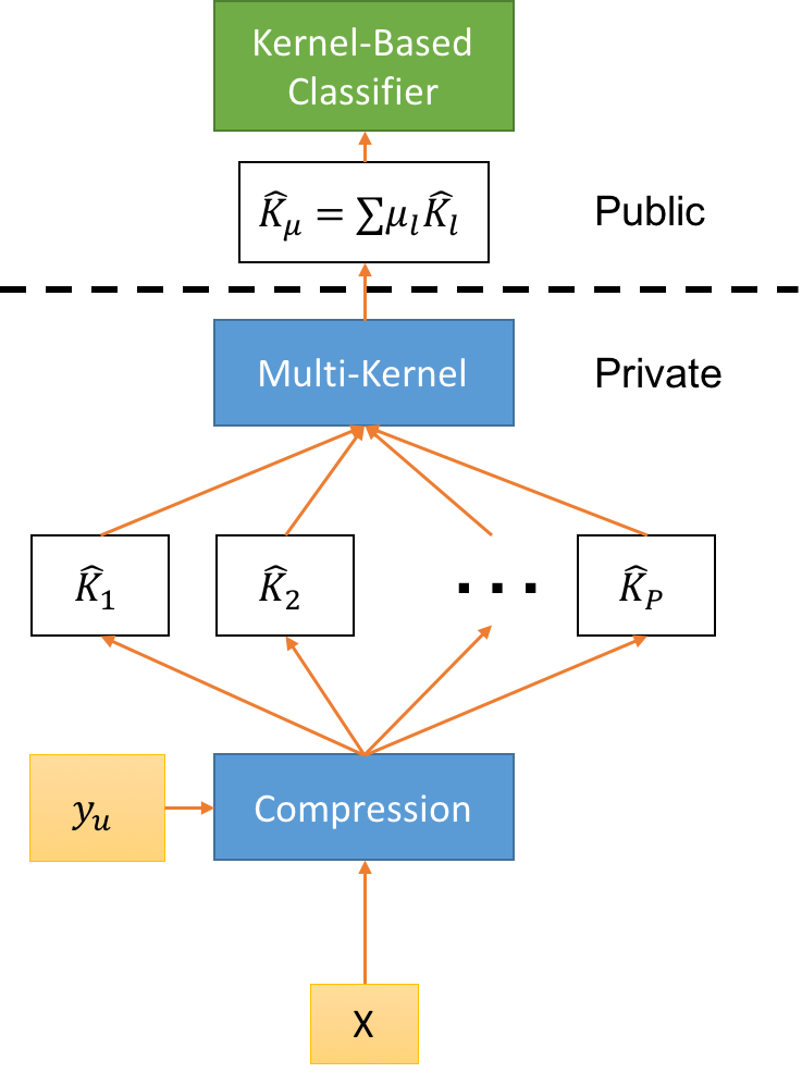
(b)

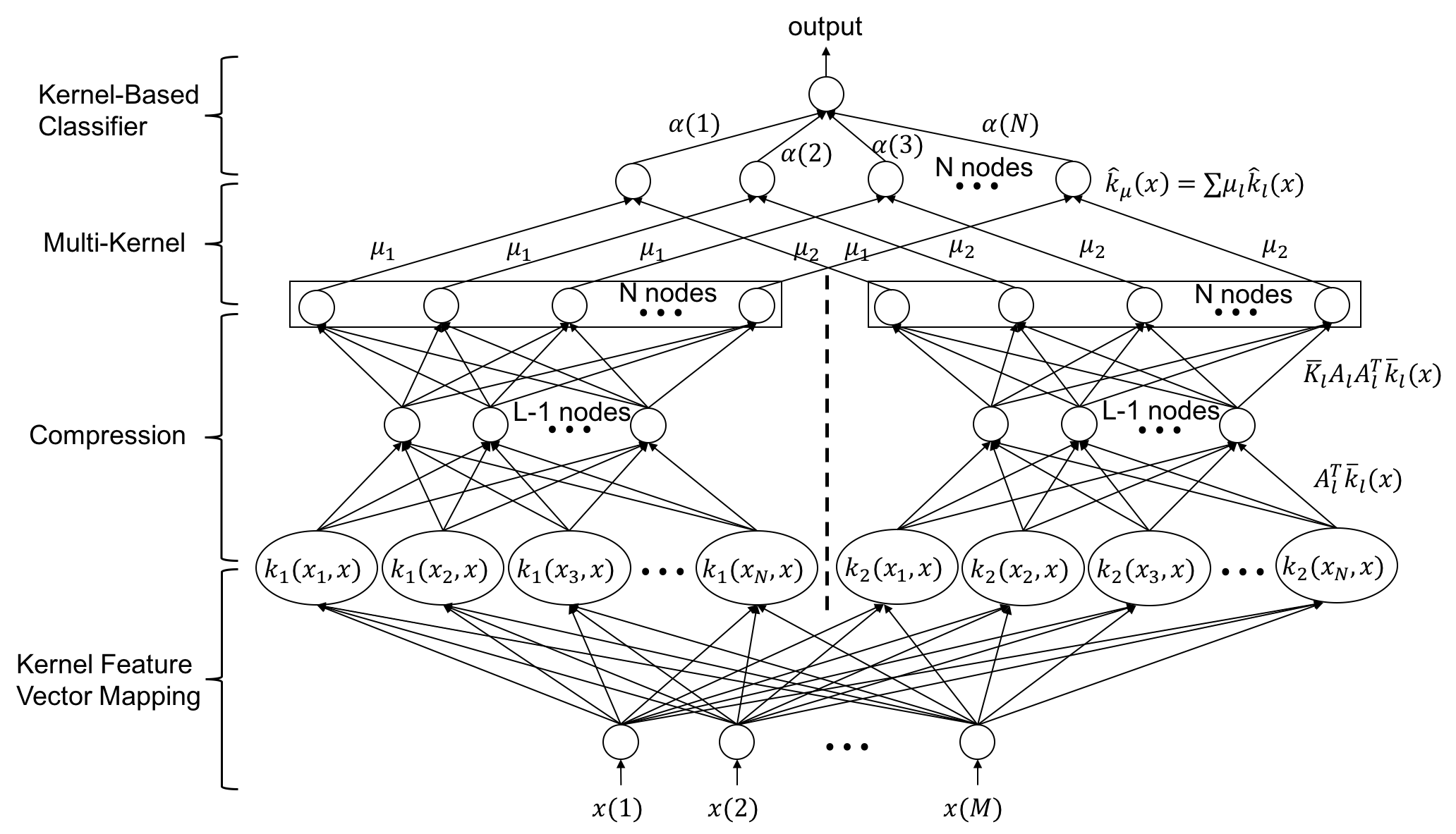
Figure 1: (a) The schematics of the compressive multi-kernel learning system. The compressive multi-kernel learning phase is considered to be private, while the classifier phase is consider to be public. (b) A neural network topology of the compressive multi-kernel learning system with two kernels. The two kernels are separated in the illustration by the dashed line.

The proposed compressive multi-kernel learning system consists of two steps – the compression step and the multi-kernel step. In the compression step, the training feature data and utility label are provided and $P$ rank-reduced kernels, $\hat{\mathbf{K}}_{1},\hat{\mathbf{K}}_{2},\ldots,\hat{\mathbf{K}}_{P}$, are produced. These rank-reduced kernels are then combined in the multi-kernel step to form the final compressive multi-kernel in the form $\hat{\mathbf{K}}_{\mu}=\sum_{l=1}^{P}\mu_{l}\hat{\mathbf{K}}_{l}$. This compressive multi-kernel is provided to the kernel-based classifier.

As common in the framework of Compressive Privacy [16, 17], the private and public spheres are separated. Both compression and multi-kernel steps are assumed to occur in the private sphere, possibly by a trusted centralized server, while the classification step is considered to be in the public sphere. Therefore, the final compressive multi-kernel $\hat{\mathbf{K}}_{\mu}$ is considered public, whereas the original feature data, $\mathbf{X}$, are private. Moreover, to evaluate the system against a strong adversary, the training data, including the feature data, the utility label and the privacy label, are assumed to be public, and the adversary is assumed to have the knowledge of the procedure of the system. The testing data are, on the other hand, considered private. Figure 1(a) summarizes the system and marks the private and public spheres.

In addition, the proposed compressive multi-kernel learning system can be visualized as a neural network illustrated in Figure 1(b). The network has four hidden layers. The first hidden layer provides the kernel feature vector mapping (as described in more detail in [1]). The second and third hidden layers act as the compression step, while the the fourth hidden layer serves as the multi-kernel step. The illustration in Figure 1(b) shows the system with two kernels, as separated by the dashed line. The last layer in the network is simply the kernel-based classifier in the system that produces a prediction as the output.

III-C The Compression Step

III-C1 Preliminary

The compression step aims at finding a low-rank approximation of each kernel matrix $\mathbf{K}_{l}$. The compressive kernel matrix considered is in the form,

$$\hat{\mathbf{K}}_{l}=\bar{\boldsymbol{\Phi}}^{T}\mathbf{L}\mathbf{L}^{T}\bar{\boldsymbol{\Phi}}$$ (2)

where $\bar{\boldsymbol{\Phi}}\in\mathbb{R}^{J\times N}$ is the centered feature data matrix in the intrinsic space as embedded by the kernel function, and $\mathbf{L}\in\mathbb{R}^{J\times Q};Q<J$ is the lossy projection matrix. In the proposed system, $\mathbf{L}$ is derived from a powerful dimensionality reduction framework called Discriminant Component Analysis (DCA) [1, 18, 19].

III-C2 Discriminant Component Analysis

Discriminant Component Analysis (DCA) aims at finding the projection matrix that maximizes the discriminant power. Given a set of training feature data and the specified target label $\{\mathbf{X},\mathbf{y}\}$, DCA utilizes the between-class scatter matrix $\mathbf{S}_{B}$, and the within-class scatter matrix $\mathbf{S}_{w}$, defined by,

$$\mathbf{S}_{B}=\sum_{l=1}^{L}N_{l}[\boldsymbol{\mu}_{l}-\boldsymbol{\mu}][\boldsymbol{\mu}_{l}-\boldsymbol{\mu}]^{T}$$ (3)

$$\mathbf{S}_{W}=\sum_{l=1}^{L}\sum_{j=1}^{N_{l}}[\mathbf{x}_{j}^{(l)}-\boldsymbol{\mu}_{l}][\mathbf{x}_{j}^{(l)}-\boldsymbol{\mu}_{l}]^{T}$$ (4)

where $L$ is the number of classes, $N_{l}$ is the number of samples in each class, $\boldsymbol{\mu}_{l}$ is the mean of the samples in the class, and $\boldsymbol{\mu}$ is the mean of the entire dataset. It can be shown that the sum of the two scatter matrices equals the overall scatter matrix of the dataset, namely,

$$\bar{\mathbf{S}}=\bar{\mathbf{X}}\bar{\mathbf{X}}^{T}=\mathbf{S}_{B}+\mathbf{S}_{W}$$ (5)

where $\bar{\mathbf{X}}$ is the centered feature data matrix.

From the two scatter matrices, the discriminant power can be defined as,

$$P(\mathbf{W})=\sum_{i=1}^{Q}\frac{\mathbf{w}_{i}^{T}[\mathbf{S}_{B}+\rho^{\prime}\mathbf{I}]\mathbf{w}_{i}}{\mathbf{w}_{i}^{T}[\bar{\mathbf{S}}+\rho\mathbf{I}]\mathbf{w}_{i}}$$ (6)

where $Q$ is the dimension of the DCA-projected subspace, $\mathbf{w}_{i}$ is each component of the projection matrix, and $\rho$ and $\rho^{\prime}$ are the ridge parameters. By imposing the canonical orthonormality that $\mathbf{W}_{DCA}^{T}[\bar{\mathbf{S}}+\rho\mathbf{I}]\mathbf{W}_{DCA}=\mathbf{I}$, the optimization formulation for DCA can be written as,

$$\mathbf{W}_{DCA}=\underset{\{\mathbf{W}:\mathbf{W}^{T}[\bar{\mathbf{S}}+\rho\mathbf{I}]\mathbf{W}=\mathbf{I}\}}{\arg\max}trace(\mathbf{W}^{T}[\mathbf{S}_{B}+\rho^{\prime}\mathbf{I}]\mathbf{W})$$ (7)

This optimization can be solved with a generalized eigenvalue problem solver and the $Q$ eigenvectors with the highest corresponding eigenvalues are chosen to form the projection matrix.

One important property of DCA is that DCA only requires $L-1$ dimensions to reach the maximum discriminant power as $\mathbf{S}_{B}$ has rank of $\leq L-1$. This property, hence, allows very high compression when $L\ll M$. Therefore, it is appropriate to call the subspace spanned by the first $L-1$ DCA components as the signal subspace, and that spanned by the rest of the components as the noise subspace. These two subspaces are obviously with respect to the specified target label used to derive the DCA components.

Another important property of DCA is that DCA satisfies the learning subspace property (LSP) [1], meaning that each component of DCA can be written as a linear combination of the training feature data, i.e., $\mathbf{w}_{i}=\bar{\mathbf{\Phi}}\mathbf{\alpha}_{i}$. Consequently, the DCA formulation can be kernelized, and the Kernel DCA (KDCA) optimizer is [1, 18],

$$\mathbf{A}_{KDCA}=\underset{\{\mathbf{A}:\mathbf{A}^{T}[\bar{\mathbf{K}}^{2}+\rho\bar{\mathbf{K}}]\mathbf{A}=\mathbf{I}\}}{\arg\max}trace(\mathbf{A}^{T}[\mathbf{K}_{B}+\rho^{\prime}\bar{\mathbf{K}}]\mathbf{A})$$ (8)

where $\mathbf{A}_{KDCA}\in\mathbb{R}^{N\times Q}$ is the projection matrix in the empirical space, and $\bar{\mathbf{K}}$, $\mathbf{K}_{B}$ and $\mathbf{K}_{W}$ are defined as follows:

$$\bar{\mathbf{K}}=\mathbf{C}_{N}\mathbf{K}\mathbf{C}_{N}$$ (9)

$$\mathbf{K}_{B}=\mathbf{C}_{N}[\sum_{l=1}^{L}N_{l}(\mathbf{k}(\boldsymbol{\mu}_{l})-\mathbf{k}(\boldsymbol{\mu}))(\mathbf{k}(\boldsymbol{\mu}_{l})-\mathbf{k}(\boldsymbol{\mu}))^{T}]\mathbf{C}_{N}$$ (10)

$$\mathbf{K}_{W}=\mathbf{C}_{N}[\sum_{l=1}^{L}\sum_{j=1}^{N_{l}}(\mathbf{k}(\mathbf{x}_{j}^{(l)})-\mathbf{k}(\boldsymbol{\mu}_{l}))(\mathbf{k}(\mathbf{x}_{j}^{(l)})-\mathbf{k}(\boldsymbol{\mu}_{l}))^{T}]\mathbf{C}_{N}$$ (11)

where

$$\mathbf{k}(\boldsymbol{\mu}_{l})=\sum_{\mathbf{x}_{j}\in\mathcal{C}_{l}}\frac{\mathbf{k}(\mathbf{x}_{j})}{N_{l}}$$

$$\mathbf{k}(\boldsymbol{\mu)}=\sum_{j=1}^{N}\frac{\mathbf{k}(\mathbf{x}_{j})}{N}$$

and $\mathbf{C}_{N}=[\mathbf{I}-\frac{1}{N}\mathbf{e}\mathbf{e}^{T}];\ \mathbf{e}=[1\ 1\cdots 1]^{T}$ is the centering matrix, $\mathbf{K}$ is the kernel matrix, and $\mathbf{k}(\mathbf{x}_{j})$ is the kernel vector. Finally, it can be shown that [1, 18]

$$\bar{\mathbf{K}}^{2}=\mathbf{K}_{B}+\mathbf{K}_{W}$$ (12)

III-C3 Compressive Kernel Matrix

The lossy projection matrix $\mathbf{L}$ is derived from DCA in the intrinsic space, $\mathbf{W}_{DCA}$. Thus, it also follows the learning subspace property, i.e., $\mathbf{L}=\bar{\mathbf{\Phi}}\mathbf{A}_{KDCA}$. This allows the compressive kernel matrix to be derived from the kernel matrix in the empirical space as follows:

$$\hat{\mathbf{K}}_{l}=\bar{\mathbf{K}}_{l}\mathbf{A}_{l}\mathbf{A}_{l}^{T}\bar{\mathbf{K}}_{l}$$ (13)

This can be seen simply by substituting $\mathbf{L}$ in Equation (2) with $\bar{\mathbf{\Phi}}\mathbf{A}_{KDCA}$ and using the fact that $\bar{\mathbf{K}}_{l}=\bar{\boldsymbol{\Phi}}_{l}^{T}\bar{\boldsymbol{\Phi}}_{l}$. The centered kernel matrix, $\bar{\mathbf{K}}_{l}$, can also be derived directly from the non-centered kernel matrix by:

$$\bar{\mathbf{K}}_{l}=\mathbf{C}_{N}\mathbf{K}_{l}\mathbf{C}_{N}$$ (14)

Given $\mathbf{A}_{l}\in\mathbb{R}^{N\times Q}$, it can be shown that rank of $\hat{\mathbf{K}}_{l}$ is $\leq Q$ [34]. Moreover, as the derivation of $\mathbf{A}_{l}$ requires only the kernel function corresponding to $\mathbf{K}_{l}$, but not those corresponding to other $\mathbf{K}_{j}$ used in the multi-kernel learning system, each $\mathbf{A}_{l}$ can be derived independently for each kernel function. The choice of $Q$ can also be chosen independently, as will be apparent in the multi-kernel step.

In the proposed system, the utility label $\mathbf{y}_{u}$ is used to derive the lossy projection matrix. This is to provide high compression when the number of utility class, $L_{u}$, is smaller than the original feature size, and at the same time, retain high classification power of the kernel matrix. It can be seen from the DCA formulation that, in fact, all discriminant power of the kernel matrix should remain when at least $L_{u}-1$ most-discriminant DCA components are used to form the lossy projection matrix. Thus, the compressive kernel matrix should provide the win-win situation in terms of privacy-utility tradeoff, namely, high compression is achieved for privacy, while maximum discriminant power remains for utility.

III-D The Multi-Kernel Step

III-D1 Preliminaries

The proposed multi-kernel is in the form,

$$\hat{\mathbf{K}}_{\mu}=\sum_{l=1}^{P}\mu_{l}\hat{\mathbf{K}}_{l}$$ (15)

where $\mu_{l}$ is the weight corresponding to each compressive kernel matrix. It is common to impose the condition $\mu_{l}\geq 0$ to guarantee that the multi-kernel is a PDS kernel [5, 6, 7, 8, 9]. This multi-kernel can also be written in the intrinsic space by considering the centered augmented embedded feature data matrix:

$$\bar{\boldsymbol{\Phi}}_{\mu}=\left[\begin{array}[]{c}\sqrt{\mu_{1}}\mathbf{L}_{1}^{T}\bar{\boldsymbol{\Phi}}_{1}\\ \sqrt{\mu_{2}}\mathbf{L}_{2}^{T}\bar{\boldsymbol{\Phi}}_{2}\\ \vdots\\ \sqrt{\mu_{P}}\mathbf{L}_{P}^{T}\bar{\boldsymbol{\Phi}}_{P}\end{array}\right]$$ (16)

It can then be shown that,

$$\hat{\mathbf{K}}_{\mu}=\bar{\boldsymbol{\Phi}}_{\mu}^{T}\bar{\boldsymbol{\Phi}}_{\mu}$$

$$\hat{\mathbf{K}}_{\mu}=\sum_{l=1}^{P}\mu_{l}\bar{\boldsymbol{\Phi}}_{l}^{T}\mathbf{L}_{l}\mathbf{L}_{l}^{T}\bar{\boldsymbol{\Phi}}_{l}=\sum_{l=1}^{P}\mu_{l}\hat{\mathbf{K}}_{l}$$

This shows that the multi-kernel in the form of Equation (15) can be considered as extending the embedded feature in the intrinsic space according to Equation (16), and hence, the additional degrees of freedom. Moreover, there is no overlap between different embedded features $\bar{\boldsymbol{\Phi}}_{l}$ and its corresponding lossy projection matrix $\mathbf{L}_{l}$, so each lossy projection matrix can be designed independently with respect to each kernel.

However, as the application of privacy is under consideration, extending the embedded feature space can come at a cost of extra information shared. Under the regime of Compressive Privacy [16, 17], this is not desirable. Hence, in the design of the multi-kernel step, the rank of the final multi-kernel should not exceed that of the original data. Given that each compressive kernel $\hat{\mathbf{K}}_{l}$ has rank of at most $Q_{l}$, it can be shown that rank of $\hat{\mathbf{K}}_{\mu}$ is $\leq\sum_{l=1}^{P}Q_{l}$ [34]. Thus, to comply with Compressive Privacy, the compressive multi-kernel has to be designed such that $\sum_{l=1}^{P}Q_{l}<M$.

III-D2 Centering and Normalization

Following the suggestion in [5], each compressive kernel should be centered and normalized before being combined. $\hat{\mathbf{K}}_{l}$ is, in fact, already centered, so only normalization is needed. The normalization is carried out such that each kernel has trace equals to one:

$$\hat{\mathbf{K}}[i,j]_{normalized}=\hat{\mathbf{K}}[i,j]/trace(\hat{\mathbf{K}})$$ (17)

where the indices $[i,j]$ indicates the element at row $i^{th}$ and column $j^{th}$.

III-D3 Signal-to-Noise Ratio for Kernel Weight Design

The design of the multi-kernel in Equation (15) involves the determination of the value of $\mu_{l}$ for each kernel. The signal-to-noise ratio (SNR) in the form of the trace-norm of the discriminant matrix, as motivated by the inter-class separability metric in Equation (31) of [16], is proposed as a new metric to decide the value of $\mu_{l}$. Specifically, the SNR is defined as,

$$SNR=\left\|[\bar{\mathbf{S}}+\rho_{snr}\mathbf{I}]^{-1}\mathbf{S}_{B}\right\|_{tr}$$ (18)

where $\bar{\mathbf{S}}$ and $\mathbf{S}_{B}$ are defined similarly to those in DCA (Section III-C2), $\rho_{snr}$ is the ridge term, and $\left\|\cdot\right\|_{tr}$ is the trace-norm defined by the sum of the singular values of the matrix. The discriminant matrix can also be derived directly in the empirical space by using the counterpart form of each scatter matrix similar to KDCA as the following:

$$SNR=\left\|[\bar{\mathbf{K}}^{2}+\rho_{snr}\mathbf{\bar{K}}]^{-1}\mathbf{K}_{B}\right\|_{tr}$$ (19)

In relation to the compressive kernels, the SNR for each compressive kernel is,

$$SNR_{l}=\left\|[\hat{\mathbf{K}}_{l}^{2}+\rho_{snr}\mathbf{\hat{K}}_{l}]^{-1}\hat{\mathbf{K}}_{B_{l}}\right\|_{tr}$$ (20)

where $\hat{\mathbf{K}}_{B_{l}}=\bar{\mathbf{K}}_{l}\mathbf{A}_{l}\mathbf{A}_{l}^{T}\mathbf{K}_{B_{l}}\mathbf{A}\mathbf{A}^{T}\bar{\mathbf{K}}_{l}$. Finally, denoting $\boldsymbol{\mu}=[\mu_{1},\mu_{2},\ldots,\mu_{P}]^{T}$ as the kernel weight vector, the value of each $\mu_{l}$ is designed to be,

$$\mu_{l}=\frac{SNR_{l}}{\left\|\boldsymbol{\mu}\right\|}$$ (21)

The design of $\boldsymbol{\mu}$ is, therefore, regularized to have norm of one.

IV Experimental Results

IV-A Datasets

The proposed system is evaluated on two datasets – Mobile Health (MHEALTH) [20, 21], and Human Activity Recognition Using Smartphones (HAR) [22]. Both datasets are related to activity recognition using mobile-sensing features, and the feature data are collected from multiple individuals, so two different labels are available – activity recognition label, and person identification label. In all experiments, activity recognition is defined as the utility classification, whereas person identification is defined as the privacy classification. Therefore, the goal of a privacy-preserving classifier is to be able to recognize the activity label with high accuracy, but identify the person with low accuracy.

The MHEALTH dataset has 23 features, and 4,800 samples are used for training, while 900 samples are left out for testing. The utility label consists of six activity classes, whereas the privacy label consists of 10 individuals. The HAR dataset has 561 features, and 5,451 samples are kept for training, while 1,080 are used for testing. The utility label has six activities, and the privacy label has 20 individuals.

IV-B Experimental Setup

In all experiments, support vector machine (SVM) is used as the classifier. The parameters of SVM are selected using cross-validation. To judge the performance of differential compressive multi-kernel methods fairly, SVM is used for all methods, and the results from single compressive kernels are also reported for comparison. Five types of kernels are used in the experiments and are defined as follows:

• Linear kernel: $\mathbf{K}_{l}(\mathbf{x}_{i},\mathbf{x}_{j})=\mathbf{x}_{i}^{T}\mathbf{x}_{j}$

• Polynomial kernel: $\mathbf{K}_{l}(\mathbf{x}_{i},\mathbf{x}_{j})=(\gamma\mathbf{x}_{i}^{T}\mathbf{x}_{j}+c_{0})^{p}$

• Radial basis function (RBF) kernel: $\mathbf{K}_{l}(\mathbf{x}_{i},\mathbf{x}_{j})=\exp(-\gamma\left\|\mathbf{x}_{i}-\mathbf{x}_{j}\right\|^{2})$

• Laplacian kernel: $\mathbf{K}_{l}(\mathbf{x}_{i},\mathbf{x}_{j})=\exp(-\gamma\left\|\mathbf{x}_{i}-\mathbf{x}_{j}\right\|_{1})$

• Sigmoid kernel: $\mathbf{K}_{l}(\mathbf{x}_{i},\mathbf{x}_{j})=\tanh(\gamma\mathbf{x}_{i}^{T}\mathbf{x}_{j}+c_{0})$

For each dataset, two sets of experiments are performed. The first experiment is on multiple RBF kernels with various gamma values. The gamma values are chosen from the set of $a\times 10^{b}$, where $a=\{1,3,5\}$ and $b=\{0,1,2,3,4,5\}$, such that, in cross-validation, the single compressive kernels are sufficiently different in individual performances, and the multi-kernel performs reasonably well . The second experiment, on the other hand, uses more than one kind of kernel. Similarly, the choice of kernels is based on sufficient difference in individual performances and reasonable multi-kernel performance in the cross-validation of all above kernels.

For comparison, four methods are investigated in each experiment.

• The compressive single kernel, where only one compressive kernel is used.

• The compressive uniform multi-kernel, which uses the uniform weight for the value of $\mu_{l}$. Hence, $\mu_{l}=1/P$ for all kernels.

• The compressive alignment-based multi-kernel, which uses the utility-target alignment maximization algorithm according to [5] on the compressive kernels to determine the value of $\mu_{l}$.

• The proposed compressive SNR-based multi-kernel, which uses the SNR score described in Section (III-D) to determine the value of $\mu_{l}$. The value of the ridge term, $\rho_{snr}$, is chosen to be zero and 0.1 across all experiments.

Finally, the details of the choice of kernels in each dataset are described as follows:

IV-B1 MHEALTH

There are six utility classes in the MHEALTH dataset ($L_{u}=6$), so in order to get the maximum discriminant power, five ($L_{u}-1=5$) DCA components are used for compression of each kernel in both experiments. Since $M=23$ for MHEALTH, three kernels are used to keep the compressive multi-kernel low-rank ($\leq 15$). The values of $\rho$ and $\rho^{\prime}$ of the DCA optimization are kept the same across all kernels in all experiments with the value of 10 and 0.0001, respectively. The kernels used in both experiments are as follows:

• In the first experiment, three RBF kernels with $\gamma=\{0.01,0.03,0.0005\}$.

• In the second experiment, a polynomial kernel with $\gamma=1.0$, $p=3$, and $c_{0}=1.0$; an RBF kernel with $\gamma=0.01$; and a Laplacian kernel with $\gamma=0.1$.

IV-B2 HAR

There are also six utility classes, so five DCA components are similarly used for compression of all kernels in both experiments. Since $M=561$ in the HAR dataset, four kernels are used (rank of the compressive multi-kernel $\leq 20$). The values of $\rho$ and $\rho^{\prime}$ of the DCA optimization are also kept constant across all kernels at 10 and 0.0001, respectively. The kernels used in both experiments are as follows:

• In the first experiment, four RBF kernels with $\gamma=\{10^{-2},10^{-3},10^{-4},10^{-5}\}$.

• In the second experiment, a linear kernel; an RBF kernel with $\gamma=10^{-3}$; a Laplacian kernel with $\gamma=0.001$; and a sigmoid kernel with $\gamma=0.001$ and $c_{0}=1$.

IV-C Results

MHEALTH: Experiment I

	Utility (%)	Privacy (%)
Random guess	16.67	10.00
Compressive single RBF kernel with $\gamma=0.01$	78.33	15.11
Compressive single RBF kernel with $\gamma=0.03$	76.00	10.44
Compressive single RBF kernel with $\gamma=0.0005$	76.33	10.22
Compressive uniform multi-RBF-kernel	81.11	11.00
Compressive alignment-based multi-RBF-kernel	84.11	10.22
Compressive SNR-based multi-RBF-kernel $\rho_{snr}=0$	82.22	13.78
Compressive SNR-based multi-RBF-kernel $\rho_{snr}=0.1$	85.67	12.00

MHEALTH: Experiment II

	Utility (%)	Privacy (%)
Random guess	16.67	10.00
Compressive single polynomial kernel	76.00	15.56
Compressive single RBF kernel	78.33	15.11
Compressive single Laplacian kernel	78.11	10.56
Compressive uniform multi-kernel	87.11	14.22
Compressive alignment-based multi-kernel	79.44	12.33
Compressive SNR-based multi-kernel $\rho_{snr}=0$	87.33	16.00
Compressive SNR-based multi-kernel $\rho_{snr}=0.1$	86.56	15.44

TABLE I: MHEALTH: utility and privacy classification accuracies

IV-C1 MHEALTH

Table I summarizes the results from both experiments on the MHEALTH dataset. In terms of privacy, both experiments show that compression is effective in providing privacy as seen by the fact that the privacy accuracy is almost at the random-guess level in all compressive single kernels. More importantly, by combining the compressive single kernels to form the compressive multi-kernel, the privacy accuracy does not significantly increase and remains almost at the random-guess level.

In terms of utility, the two compressive SNR-based multi-kernels show significant improvement in the utility accuracy in both experiments. Specifically, in the first experiment, the compressive SNR-based multi-kernel with $\rho_{snr}=0.1$ yields the best result with 7.34% improvement over the compressive single kernel; 4.56% over the compressive uniform multi-kernel; and 1.56% over the compressive alignment-based multi-kernel. Meanwhile, in the second experiment, the compressive SNR-based multi-kernel with $\rho_{snr}=0$ performs best with 9.00% higher utility accuracy than the compressive single kernel; 0.22% higher than the compressive uniform multi-kernel; and 7.89% higher than the compressive alignment-based multi-kernel.

HAR: Experiment I

	Utility (%)	Privacy (%)
Random guess	16.67	5.00
Compressive single RBF kernel with $\gamma=10^{-2}$	84.72	5.00
Compressive single RBF kernel with $\gamma=10^{-3}$	86.20	6.48
Compressive single RBF kernel with $\gamma=10^{-4}$	89.26	6.85
Compressive single RBF kernel with $\gamma=10^{-5}$	83.70	5.00
Compressive uniform multi-RBF-kernel	89.63	6.39
Compressive alignment-based multi-RBF-kernel	90.19	5.00
Compressive SNR-based multi-RBF-kernel $\rho_{snr}=0$	89.35	6.85
Compressive SNR-based multi-RBF-kernel $\rho_{snr}=0.1$	90.93	5.00

HAR: Experiment II

	Utility (%)	Privacy (%)
Random guess	16.67	5.00
Compressive single linear kernel	51.02	5.19
Compressive single RBF kernel	86.20	6.48
Compressive single Laplacian kernel	90.83	5.00
Compressive single sigmoid kernel	82.59	7.04
Compressive uniform multi-kernel	90.65	6.57
Compressive alignment-based multi-kernel	91.30	6.57
Compressive SNR-based multi-kernel $\rho_{snr}=0$	89.35	6.85
Compressive SNR-based multi-kernel $\rho_{snr}=0.1$	91.39	5.00

TABLE II: HAR: utility and privacy classification accuracies

IV-C2 HAR

Table II summarizes the results from both experiments on the HAR dataset. In terms of privacy, both experiments show that compression is very effective in providing privacy as the privacy accuracy is equivalent or close to random guess in all compressive single kernels. Similarly, by combining the compressive single kernels to form the compressive multi-kernel, the privacy accuracy does not increase and remains at or close to random guess.

In terms of utility, the compressive multi-kernel, again, shows improvement in both experiments on the HAR dataset. The compressive SNR-based multi-kernel with $\rho_{snr}=0.1$, specifically, yields the best performance in both experiments by improving upon the compressive single kernel by at least 1.67% and 0.56%; upon the compressive uniform multi-kernel by 1.30% and 0.74%; and upon the compressive alignment-based multi-kernel in both experiments by 0.74% and 0.09%.

V Discussion and Future Works

V-A Compression for Privacy

The results from the evaluation confirm that the compression step indeed provides privacy protection as the privacy classification accuracy is around random guess in all experiments. This is true even when multiple compressive kernels are used. This success in privacy-preservation is achievable from the fact that large amount of information is loss during the compression step.

The compression step is actually general as other dimensionality reduction techniques can also be used. Future work can be carried out on studying the effect on the choice of the compression method. Some possible ideas for future work are the following:

• Principal Component Analysis (PCA) may be used to maximize data reconstruction quality when the utility and privacy labels are not known in advance.

• Desensitized RDCA method [17] may be used when the privacy label is known at the time of compression but the utility label is not.

• Utility-to-privacy ratio [35, 16] maybe used when both utility and privacy labels are known.

V-B Multi-Kernel for Utility (and Privacy)

In the current system, the multi-kernel step is primarily for utility improvement. The results from the evaluation conform with the goal. Especially, the SNR-based kernel weight score proposed is shown to be fairly effective and improving upon the state-of-the-art. Nevertheless, the current work primarily focuses on using the multi-kernel weight optimization for enhancing utility only, but as the application of privacy-preserving machine learning involves maximizing utility, while minimizing privacy, it is interesting to seek an alternative optimization criterion that fits this objective.

Fortunately, the SNR score can be extended to such setting by considering the utility-to-privacy ratio similar to that in [35, 16]. By utilizing both the utility label $\mathbf{y}_{u}$ and privacy label $\mathbf{y}_{p}$, the utility-to-privacy ratio can be defined as,

$$UPR=\left\|[\mathbf{S}_{B_{P}}+\rho_{upr}\mathbf{I}]^{-1}\mathbf{S}_{B_{U}}\right\|_{tr}$$ (22)

where $\mathbf{S}_{B_{U}}$ is the between-class scatter matrix derived from $\mathbf{y}_{u}$, $\mathbf{S}_{B_{P}}$ is the between-class scatter matrix derived from $\mathbf{y}_{p}$, and $\rho_{upr}$ is, again, the ridge term. Naturally, the utility-to-privacy ratio can also be derived in the empirical space:

$$UPR=\left\|[\mathbf{K}_{B_{P}}+\rho_{upr}\mathbf{\bar{K}}]^{-1}\mathbf{K}_{B_{U}}\right\|_{tr}$$ (23)

where $\mathbf{K}_{B_{U}}$ is the counterpart of $\mathbf{S}_{B_{U}}$ and $\mathbf{K}_{B_{P}}$ is the counterpart of $\mathbf{S}_{B_{P}}$ in the empirical space.

Alternatively, the alignment approach in [6, 7] can also be extended to consider both utility and privacy together by defining the alignments between the multi-kernel matrix and the targeted utility and privacy labels, respectively, as:

$$A_{u}(\hat{\mathbf{K}}_{\mu},\mathbf{y}_{u}\mathbf{y}_{u}^{T})=\bigl{\langle}\hat{\mathbf{K}}_{\mu},\mathbf{y}_{u}\mathbf{y}_{u}^{T}\bigr{\rangle}_{F}/\bigl{\|}\hat{\mathbf{K}}_{\mu}\bigr{\|}_{F}$$ (24)

$$A_{p}(\hat{\mathbf{K}}_{\mu},\mathbf{y}_{p}\mathbf{y}_{p}^{T})=\bigl{\langle}\hat{\mathbf{K}}_{\mu},\mathbf{y}_{p}\mathbf{y}_{p}^{T}\bigr{\rangle}_{F}/\bigl{\|}\hat{\mathbf{K}}_{\mu}\bigr{\|}_{F}$$ (25)

Then, following the line of thought in the Differential Utility/Cost Analysis (DUCA) formulation [16], the utility-to-privacy ratio can be maximized as the following:

$$\boldsymbol{\mu}=\underset{\boldsymbol{\mu}:\left\|\boldsymbol{\mu}\right\|=1,\boldsymbol{\mu}\geq 0}{\arg\max}\frac{A_{u}(\hat{\mathbf{K}}_{\mu},\mathbf{y}_{u}\mathbf{y}_{u}^{T})}{A_{p}(\hat{\mathbf{K}}_{\mu},\mathbf{y}_{p}\mathbf{y}_{p}^{T})}=\underset{\boldsymbol{\mu}:\left\|\boldsymbol{\mu}\right\|=1,\boldsymbol{\mu}\geq 0}{\arg\max}\frac{\bigl{\langle}\hat{\mathbf{K}}_{\mu},\mathbf{y}_{u}\mathbf{y}_{u}^{T}\bigr{\rangle}_{F}}{\bigl{\langle}\hat{\mathbf{K}}_{\mu},\mathbf{y}_{p}\mathbf{y}_{p}^{T}\bigr{\rangle}_{F}}$$

This optimization criterion can be formulated into a simple quadratic programming problem. First, defining the following two vectors:

$$\mathbf{a}_{u}=[\mathbf{y}_{u}^{T}\hat{\mathbf{K}}_{1}\mathbf{y}_{u},\ \mathbf{y}_{u}^{T}\hat{\mathbf{K}}_{2}\mathbf{y}_{u},\ldots,\ \mathbf{y}_{u}^{T}\hat{\mathbf{K}}_{P}\mathbf{y}_{u}]^{T}$$

$$\mathbf{a}_{p}=[\mathbf{y}_{p}^{T}\hat{\mathbf{K}}_{1}\mathbf{y}_{p},\ \mathbf{y}_{p}^{T}\hat{\mathbf{K}}_{2}\mathbf{y}_{p},\ldots,\ \mathbf{y}_{p}^{T}\hat{\mathbf{K}}_{P}\mathbf{y}_{p}]^{T}$$

Then, it can be shown that the solution $\boldsymbol{\mu}^{*}$ is given by $\boldsymbol{\mu}^{*}=\mathbf{v}^{*}/\left\|\mathbf{v}^{*}\right\|$, where $\mathbf{v}^{*}$ is the solution of the following quadratic program:

$$\min_{\mathbf{v}\geq 0}\mathbf{v}^{T}\mathbf{a}_{p}\mathbf{a}_{p}^{T}\mathbf{v}-2\mathbf{v}^{T}\mathbf{a}_{u}$$ (26)

The proof of this proposition directly follows the proof of the alignment maximization algorithm in Proposition 3 of [6].

These two optimization criteria will be an interesting formulation for future study, especially for the case when compression alone is not sufficient for privacy protection.

V-C Multiple Utility Labels

One advantage of the multi-kernel in the form of Equation (15) is the independence among the kernels, which, as a result, allows each kernel to be designed for different purposes. This lends itself nicely to the application when there are more than one utility label. For example, different kinds of kernel can be chosen for each utility label, and the multi-kernel should then be useful for more than one utility simultaneously. Alternatively, under the compressive kernel scheme, the DCA-derived lossy projection matrix used for kernel compression can be derived from DCA with respect to different utility labels for different kernels. This would allow the multi-kernel to be applicable to more than one utility label and possible reduce conflict in the compression design.

VI Conclusion

In addressing the challenge problem of privacy-preserving machine learning, this work is built upon two regimes – Compressive Privacy for privacy protection, and multi-kernel method for utility maximization. The tasks considered are the classifications of the utility and privacy labels. The proposed compressive multi-kernel method consists of two steps – compression and multi-kernel. In the compression step, each kernel is compressed using the DCA lossy projection matrix. In the multi-kernel step, multiple compressive kernels are combined based on the proposed SNR score.

The proposed method is evaluated on the utility and privacy classification tasks using two datasets – MHEALTH and HAR. The results show that the compression step effectively provides privacy protection by reducing the privacy accuracy to almost random guess in all experiments. On the other hand, the compressive multi-kernel shows improvement in the utility accuracy over the single compressive kernels in both datasets. More importantly, the proposed SNR-based multi-kernel shows enhancing performance in comparison to the previous uniform and alignment-based methods. Overall, this work offers a promising direction to the challenging problem of privacy-preserving machine learning.

References

- [1] S. Y. Kung, Kernel Methods and Machine Learning. Cambridge, UK: Cambridge University Press, 2014.
- [2] B. Scholkopf and A. J. Smola, Learning with kernels: support vector machines, regularization, optimization, and beyond. MIT press, 2002.
- [3] J. Shawe-Taylor and N. Cristianini, Kernel methods for pattern analysis. Cambridge university press, 2004.
- [4] K. Xu, H. Yue, L. Guo, Y. Guo, and Y. Fang, “Privacy-preserving machine learning algorithms for big data systems,” in ICDCS 2015. IEEE, 2015, pp. 318–327.
- [5] C. Cortes, M. Mohri, and A. Rostamizadeh, “Two-stage learning kernel algorithms,” in Proceedings of the 27th ICML, 2010.
- [6] ——, “Learning non-linear combinations of kernels,” in Advances in neural information processing systems, 2009, pp. 396–404.
- [7] G. R. Lanckriet, N. Cristianini, P. Bartlett, L. E. Ghaoui, and M. I. Jordan, “Learning the kernel matrix with semidefinite programming,” Journal of Machine learning research, vol. 5, no. Jan, pp. 27–72, 2004.
- [8] C. Cortes, M. Mohri, and A. Rostamizadeh, “L2 regularization for learning kernels,” in Proceedings of the 25th UAI. AUAI Press, 2009.
- [9] F. R. Bach, G. R. Lanckriet, and M. I. Jordan, “Multiple kernel learning, conic duality, and the smo algorithm,” in Proceedings of the 21st ICML. ACM, 2004, p. 6.
- [10] C. Cortes, “Can learning kernels help performance,” in Invited talk at ICML 2009, 2009.
- [11] P. R. Clearinghouse, “Chronology of data breaches,” http://www.privacyrights.org/data-breach, 2016.
- [12] A. Narayanan, H. Paskov, N. Z. Gong, J. Bethencourt, E. Stefanov, E. C. R. Shin, and D. Song, “On the feasibility of internet-scale author identification,” in 2012 IEEE S&P. IEEE, 2012, pp. 300–314.
- [13] J. A. Calandrino, A. Kilzer, A. Narayanan, E. W. Felten, and V. Shmatikov, “”you might also like:” privacy risks of collaborative filtering,” in 2011 IEEE S&P. IEEE, 2011, pp. 231–246.
- [14] M. Barbaro and T. Z. Jr., “A face is exposed for aol searcher no. 4417749,” http://www.nytimes.com/2006/08/09/technology/09aol.html, Aug 9, 2006 2006.
- [15] A. Narayanan and V. Shmatikov, “Robust de-anonymization of large sparse datasets,” in IEEE S&P 2008. IEEE, 2008, pp. 111–125.
- [16] S. Kung, “Compressive privacy: From informationestimation theory to machine learning [lecture notes],” IEEE Signal Processing Magazine, vol. 34, no. 1, pp. 94–112, 2017.
- [17] S. Kung, T. Chanyaswad, J. M. Chang, and P. Wu, “Collaborative PCA/DCA learning methods for compressive privacy,” ACM Trans.Embed.Comput.Syst.
- [18] S.-Y. Kung, “Discriminant component analysis for privacy protection and visualization of big data,” Multimedia Tools and Applications, pp. 1–36, 2015.
- [19] T. Chanyaswad, J. M. Chang, P. Mittal, and S. Kung, “Discriminant-component eigenfaces for privacy-preserving face recognition,” in MLSP 2016. IEEE, 2016, pp. 1–6.
- [20] O. Banos, R. Garcia, J. A. Holgado-Terriza, M. Damas, H. Pomares, I. Rojas, A. Saez, and C. Villalonga, “mhealthdroid: a novel framework for agile development of mobile health applications,” in International Workshop on Ambient Assisted Living. Springer, 2014, pp. 91–98.
- [21] O. Banos, C. Villalonga, R. Garcia, A. Saez, M. Damas, J. A. Holgado-Terriza, S. Lee, H. Pomares, and I. Rojas, “Design, implementation and validation of a novel open framework for agile development of mobile health applications,” Biomedical engineering online, vol. 14, no. 2, p. 1, 2015.
- [22] D. Anguita, A. Ghio, L. Oneto, X. Parra, and J. L. Reyes-Ortiz, “A public domain dataset for human activity recognition using smartphones.” in ESANN, 2013.
- [23] P. Gehler and S. Nowozin, “Infinite kernel learning,” in NIPS Workshop on Kernel Learning: Automatic Selection of Optimal Kernels, 2008.
- [24] C. A. Micchelli and M. Pontil, “Learning the kernel function via regularization,” Journal of Machine Learning Research, vol. 6, no. Jul, pp. 1099–1125, 2005.
- [25] A. Argyriou, C. A. Micchelli, and M. Pontil, “Learning convex combinations of continuously parameterized basic kernels,” in International Conference on Computational Learning Theory. Springer, 2005, pp. 338–352.
- [26] A. Zien and C. S. Ong, “Multiclass multiple kernel learning,” in Proceedings of the 24th ICML. ACM, 2007, pp. 1191–1198.
- [27] D. P. Lewis, T. Jebara, and W. S. Noble, “Nonstationary kernel combination,” in Proceedings of the 23rd ICML. ACM, 2006.
- [28] F. R. Bach, “Exploring large feature spaces with hierarchical multiple kernel learning,” in Advances in neural information processing systems, 2009, pp. 105–112.
- [29] Y.-Y. Lin, T.-L. Liu, and C.-S. Fuh, “Multiple kernel learning for dimensionality reduction,” IEEE Transactions on Pattern Analysis and Machine Intelligence, vol. 33, no. 6, pp. 1147–1160, 2011.
- [30] S. S. Bucak, R. Jin, and A. K. Jain, “Multiple kernel learning for visual object recognition: A review,” IEEE Transactions on Pattern Analysis and Machine Intelligence, vol. 36, no. 7, pp. 1354–1369, 2014.
- [31] C. Hinrichs, V. Singh, J. Peng, and S. Johnson, “Q-mkl: Matrix-induced regularization in multi-kernel learning with applications to neuroimaging,” in Advances in neural information processing systems, 2012, pp. 1421–1429.
- [32] N. Subrahmanya and Y. C. Shin, “Sparse multiple kernel learning for signal processing applications,” IEEE Transactions on Pattern Analysis and Machine Intelligence, vol. 32, no. 5, pp. 788–798, 2010.
- [33] F. Wang, L. Liu, and C. Dou, “Stock market volatility prediction: a service-oriented multi-kernel learning approach,” in SCC 2012. IEEE, 2012, pp. 49–56.
- [34] R. A. Horn and C. R. Johnson, Matrix analysis. Cambridge university press, 2012.
- [35] K. Diamantaras and S.-Y. Kung, “Data privacy protection by kernel subspace projection and generalized eigenvalue decomposition,” in MLSP 2016. IEEE, 2016, pp. 1–6.