Semileptonic decays $D\to\eta\pi e^{+}\nu_{e}$ in the $a_{0}(980)$ region

Abstract

The mechanism of the four-quark production of the light scalar isovector four-quark state $a_{0}(980)$ in the $D\to\eta\pi e^{+}\nu_{e}$ decays is discussed. It is shown that the characteristic features of the shape of the $\eta\pi$ mass spectra expected in our scheme can serve as the indicator of the production mechanism and internal structure of the $a_{0}(980)$ resonance.

I INTRODUCTION

Semileptonic decays of $D$ and $B$ mesons into $e^{+}\nu_{e}$ and a pair of pseudoscalar mesons are a good laboratory for studying the quark structure of light scalar mesons CLEO09b ; WL10 ; Pe10 ; Fa11 ; AK12 ; PDG2020 . The first important experiments in this direction were carried out by the Collaborations BABAR, on the decay $D^{+}_{s}\to f_{0}(980)e^{+}\nu_{e}\to K^{+}K^{-}e^{+}\nu_{e}$ BABAR08 , CLEO, on the decay $D^{+}_{s}\to f_{0}(980)e^{+}\nu_{e}\to\pi^{+}\pi^{-}e^{+}\nu_{e}$ CLEO09a ; CLEO09b , and BESIII, on the decays $D^{0}\to a_{0}(980)^{-}e^{+}\nu_{e}\to\eta\pi^{-}e^{+}\nu_{e}$ BESIII18 , $D^{+}\to a_{0}(980)^{0}e^{+}\nu_{e}\to\eta\pi^{0}e^{+}\nu_{e}$ BESIII18 , $D^{+}\to f_{0}(500)e^{+}\nu_{e}\to\pi^{+}\pi^{-}e^{+}\nu_{e}$ BESIII19 , and $D^{+}_{s}\to a_{0}(980)^{0}e^{+}\nu_{e}\to\pi^{0}\eta e^{+}\nu_{e}$ BESIII21 . Theoretical studies of these decays and phenomenological data processing have been carried out especially recently very intensively WL10 ; Pe10 ; Fa11 ; AK12 ; AK14 ; SO15 ; Sh17 ; Ch17 ; AK18 ; AK19 ; Ac20 ; So20 ; AKS20 ; Sh21a ; Sh21b . In many ways, their goal is to find new evidence in favor of the supposed exotic four-quark ($q^{2}\bar{q}^{2}$) structure of the $f_{0}(500)$, $f_{0}(980)$, and $a_{0}(980)$ resonances or indications that contradict this. They also contain the descriptions of the mass distributions of pseudoscalar meson pairs and calculations of the relative and absolute values of the probabilities of the indicated semileptonic decays of $D$ and $B$ mesons, taking into account the requirements of the unitarity condition.

We continue the study of the decays $D^{0}\to d\bar{u}e^{+}\nu_{e}\to a_{0}(980)^{-}e^{+}\nu_{e}\to\eta\pi^{-}e^{+}\nu_{e}$ and $D^{+}\to d\bar{d}e^{+}\nu_{e}\to a_{0}(980)^{0}e^{+}\nu_{e}\to\eta\pi^{0}e^{+}\nu_{e}$ started in Ref. AK18 . These decays are interesting in that they provide direct probing of constituent two-quark $d\bar{u}$ and $(u\bar{u}-d\bar{d})/\sqrt{2}$ components in the wave functions of the $a_{0}(980)^{-}$ and $a_{0}(980)^{0}$ mesons, respectively AK12 . In Ref. AK18 the mass spectra of $\eta\pi$ pairs were presented for the case when the $a_{0}(980)$ states have no two-quark components at all. It was assumed that the production of the four-quark $a_{0}(980)$ state occurs via its mixing with the heavy $q\bar{q}$ state $a^{\prime}_{0}(1400)$, due to their common decay channels into $\eta\pi$, $\eta^{\prime}\pi$, and $K\bar{K}$. Here we also assume that the $a_{0}(980)$ meson has a four-quark structure Ja77 ; AI89 . The difference is that we consider the mechanism of four-quark fluctuations of $d\bar{u}$ and $d\bar{d}$ sources, $d\bar{u}\to d\bar{q}q\bar{u}$ and $d\bar{d}\to d\bar{q}q\bar{d}$, which in the language of two-body hadronic states means the creation of the $\eta\pi$, $\eta^{\prime}\pi$, and $K\bar{K}$ pairs, which are then dressed by strong interactions in the final state. We elucidate the characteristic features of this mechanism and do not involve in consideration a heavy state of the $a^{\prime}_{0}(1400)$ type. A similar approach was used in Refs. AKS20 ; Ac21 to describe the CLEO CLEO09b and BESIII BESIII19 data on the decays $D^{+}_{s}\to f_{0}(980)e^{+}\nu_{e}\to\pi^{+}\pi^{-}e^{+}\nu_{e}$ and $D^{+}\to f_{0}(500)e^{+}\nu_{e}\to\pi^{+}\pi^{-}e^{+}\nu_{e}$ as well as the BESIII Ab15 data on the $J/\psi\to\gamma\pi^{0}\pi^{0}$ decay in the $\pi^{0}\pi^{0}$ invariant mass region from the threshold up to 1 GeV.

This paper is organized as follows. In Sec. II after a brief discussion of the experimental situation, the general formulas are given for the widths of semileptonic decays $D^{0}\to\eta\pi^{-}e^{+}\nu_{e}$ and $D^{+}\to\eta\pi^{0}e^{+}\nu_{e}$ with the production of the $\eta\pi$ system in the $S$ wave. Section III is devoted to a discussion of the four-quark mechanism of the $a_{0}(980)$ resonance production in the $D\to\eta\pi e^{+}\nu_{e}$ decays. We show that the characteristic features of the shape of the $\eta\pi^{-}$ and $\eta\pi^{0}$ mass spectra expected in our scheme can serve as an indicator of the production mechanism and internal structure of the $a_{0}(980)$ state. In Sec. IV we discuss the decays $D^{0}\to K^{0}K^{-}e^{+}\nu_{e}$, $D^{+}\to K^{0}\bar{K}^{0}e^{+}\nu_{e}$, and $D^{+}\to K^{+}K^{-}e^{+}\nu_{e}$ which also are of interest in connection with the production of light scalar mesons. However, these decays are strongly suppressed by the phase space near the $K\bar{K}$ thresholds and their experimental investigations are little realistic at present. In Sec. V the conclusions are briefly formulated.

II BESIII data and decay widths

Recently, the BESIII Collaboration BESIII18 obtained the first data on semileptonic decays $D^{0}\to a_{0}(980)^{-}e^{+}\nu_{e}$ and $D^{+}\to a_{0}(980)^{0}e^{+}\nu_{e}$ using the reaction $e^{+}e^{-}\to\psi(3770)\to D\bar{D}$ at a center-of-mass energy of 3.773 GeV and the tagged $D$ meson technique Ba86 . They selected $25.7^{+6.4}_{-5.7}$ signal events for $D^{0}\to a_{0}(980)^{-}e^{+}\nu_{e}$ and $10.2^{+5.0}_{-4.1}$ signal events for $D^{+}\to a_{0}(980)^{0}e^{+}\nu_{e}$. The statistical significance of signal is $6.4\sigma$ for $D^{0}\to a_{0}(980)^{-}e^{+}\nu_{e}$ and $2.9\sigma$ for $D^{+}\to a_{0}(980)^{0}e^{+}\nu_{e}$. The absolute branching fractions and the ratio of decay widths were determined to be BESIII18

$$\mathcal{B}(D^{0}\to a_{0}(980)^{-}e^{+}\nu_{e})\times\mathcal{B}(a_{0}(980)^{-}\to\eta\pi^{-}) = [1.33^{+0.33}_{-0.29}(\mbox{stat})\pm 0.09(\mbox{syst})]\times 10^{-4},$$ (1)

$$\mathcal{B}(D^{+}\to a_{0}(980)^{0}e^{+}\nu_{e})\times\mathcal{B}(a_{0}(980)^{0}\to\eta\pi^{0}) = [1.66^{+0.81}_{-0.66}(\mbox{stat})\pm 0.11(\mbox{syst})]\times 10^{-4},$$ (2)

$$\frac{\Gamma(D^{0}\to a_{0}(980)^{-}e^{+}\nu_{e})}{\Gamma(D^{+}\to a_{0}(980)^{0}e^{+}\nu_{e})} = 2.03\pm 0.95\pm 0.06.$$ (3)

When obtaining Eq. (3), it was assumed that $\mathcal{B}(a_{0}(980)^{-}\to\eta\pi^{-})=\mathcal{B}(a_{0}(980)^{0}\to\eta\pi^{0})$.

In the measured $\eta\pi$ mass spectra in the range of the invariant mass of the $\eta\pi$ system, $m_{\eta\pi}\equiv\sqrt{s}$, from $0.7$ GeV to $1.3$ GeV, there is a complex configuration of background contributions BESIII18 (see Fig. 1).

Figure 1: The $\eta\pi$ mass spectra (a) for $D^{0}\to(a_{0}(980)^{-}\to\eta\pi^{-})e^{+}\nu_{e}$ and (b) for $D^{+}\to(a_{0}(980)^{0}\to\eta\pi^{0})e^{+}\nu_{e}$. Points with error bars are the BESIII data BESIII18 . The dashed curves show the sum of the background contributions defined by BESIII.

A small number of signal events, a noticeable background and a wide step in $\sqrt{s}$ (equal to $50$ MeV) do not allow us to clearly see in the $\eta\pi^{-}$ and $\eta\pi^{0}$ mass spectra the line shape of the $a_{0}(980)$ resonance. It is clear that the high statistics on the decays $D\to a_{0}(980)e^{+}\nu_{e}$ is highly demanded by the physics of light scalar mesons.

Let us write the differential width for the $D^{0}=c\bar{u}$ decay into $\eta\pi^{-}e^{+}\nu_{e}$ in the form (see, for example, Refs. CLEO09b ; BESIII19 ; Sa11 )

$$\frac{d^{2}\Gamma_{D^{0}\to d\bar{u}e^{+}\nu_{e}\to(S^{-}\to\eta\pi^{-})e^{+}\nu_{e}}(s,q^{2})}{d\sqrt{s}\,dq^{2}}=\frac{G^{2}_{F}|V_{cd}|^{2}}{24\pi^{3}}p^{3}_{\eta\pi^{-}}(m_{D^{0}},q^{2},s)|f^{D^{0}}_{+}(q^{2})|^{2}\frac{2\sqrt{s}}{\pi}|F^{D^{0}}_{d\bar{u}\to S^{-}\to\eta\pi^{-}}(s)|^{2}\rho_{\eta\pi^{-}}(s),$$ (4)

where $s$ and $q^{2}$ are the invariant mass squared of the virtual scalar state $S^{-}$ (or the $S$-wave $\eta\pi^{-}$ system) and the $e^{+}\nu_{e}$ system, respectively; $G_{F}$ is the Fermi constant, $|V_{cd}|=0.221\pm 0.004$ is a Cabibbo-Kobayshi-Maskawa matrix element PDG2020 ; $p_{\eta\pi^{-}}$ is the magnitude of the three-momentum of the $\eta\pi^{-}$ system in the $D^{0}$ meson rest frame,

$$p_{\eta\pi^{-}}(m_{D^{0}},q^{2},s)=\sqrt{[(m_{D^{0}}-\sqrt{s})^{2}-q^{2}][(m_{D^{0}}+\sqrt{s})^{2}-q^{2}]}/(2m_{D^{0}}),$$ (5)

and $\rho_{\eta\pi^{-}}(s)=\sqrt{[s-(m_{\eta}+m_{\pi^{-}})^{2}][s-(m_{\eta}-m_{\pi^{-}})^{2}]}/s$. In a simplest pole approximation, the form factor $f^{D^{0}}_{+}(q^{2})$ has the form CLEO09b ; BESIII19 ; Sa11

$$f^{D^{0}}_{+}(q^{2})=\frac{f^{D^{0}}_{+}(0)}{1-q^{2}/m^{2}_{A}},$$ (6)

where we put $m_{A}=m_{D^{+}_{1}}=2.42$ GeV PDG2020 (in principle, $m_{A}$ can be extracted from the data by fitting). The amplitude $F^{D^{0}}_{d\bar{u}\to S^{-}\to\eta\pi^{-}}(s)$ describes the formation and decay into $\eta\pi^{-}$ of the virtual scalar isovector state $S^{-}$ produced in the $D^{0}\to\eta\pi^{-}e^{+}\nu_{e}$ decay. The $\eta\pi^{-}$ invariant mass distribution integrated over the full $q^{2}$ region is given by

$$\frac{d\Gamma_{D^{0}\to d\bar{u}e^{+}\nu_{e}\to(S^{-}\to\eta\pi^{-})e^{+}\nu_{e}}(s)}{d\sqrt{s}}=\frac{G^{2}_{F}|V_{cq}|^{2}}{24\pi^{3}}|f^{D^{0}}_{+}(0)|^{2}\,\Phi(m_{D^{0}},m_{A},s)\frac{2\sqrt{s}}{\pi}|F^{D^{0}}_{d\bar{u}\to S^{-}\to\eta\pi^{-}}(s)|^{2}\rho_{\eta\pi^{-}}(s),$$ (7)

where the function $\Phi(m_{D^{0}},m_{A},s)$ is

$$\Phi(m_{D^{0}},m_{A},s)=\int\limits_{0}^{(m_{D^{0}}-\sqrt{s})^{2}}\frac{p^{3}_{\eta\pi^{-}}(m_{D^{0}},q^{2},s)}{|1-q^{2}/m^{2}_{A}|^{2}}\,dq^{2}.$$ (8)

As can be seen from Fig. 2, it notably enhances the $\eta\pi^{-}$ mass spectrum as $\sqrt{s}$ decreases.

Figure 2: The function $\Phi(m_{D^{0}},m_{A},s)$ at $m_{A}=m_{D^{+}_{1}}=2.42$ GeV.

The differential widths of the semileptonic decay of the $D^{+}=c\bar{d}$ meson into the $S$-wave $\eta\pi^{0}$ system are described by the formulas similar to Eqs. (4)–(8).

III Four-quark production mechanism of the four-quark $a_{0}(980)$ resonance

We start with the semileptonic decay of the $D^{0}=c\bar{u}$ meson $D^{0}\to d\bar{u}e^{+}\nu_{e}\to(S^{-}\to\eta\pi^{-})e^{+}\nu_{e}$. Let, as a result of radiation of the lepton pair $e^{+}\nu_{e}$ by the valence $c$ quark included in $D^{0}$, a virtual system of $d$ and $\bar{u}$ quarks in the scalar state is produced. Consider the four-quark fluctuations of such a $d\bar{u}$ source, $d\bar{u}\to d\bar{q}q\bar{u}$, corresponding to the diagram shown in Fig. 3. The limitation to this type of fluctuations is related to the Okubo-Zweiga-Iizuka (OZI) rule Ok63 ; Ok78 ; Zw80 ; Ii66 , according to which other fluctuations such as annihilation or creation of $q\bar{q}$ pairs, corresponding to the so-called “hair-pin” diagrams, are suppressed.

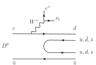
Figure 3: The OZI allowed four-quark fluctuations of the $d\bar{u}$ source, $d\bar{u}\to d\bar{q}q\bar{u}$.

In the language of hadronic states the seed four-quark fluctuations $d\bar{u}\to d\bar{q}q\bar{u}$ imply the production of $\eta\pi^{-}$, $\eta^{\prime}\pi^{-}$, and $K^{0}K^{-}$ meson pairs. As a first approximation, we assume that the amplitude of the $d\bar{u}\to d\bar{q}q\bar{u}$ transition, which we denote by $g_{0}$, does not depend on the flavor of the light $q$ quark. Then for the hadron production constants $g_{d\bar{u}\eta\pi^{-}}$, $g_{d\bar{u}\eta^{\prime}\pi^{-}}$, and $g_{d\bar{u}K^{0}K^{-}}$ the following relations hold:

$$g_{d\bar{u}\eta\pi^{-}}=\sqrt{2}g_{0}\sin(\theta_{i}-\theta_{p}),\ \ \ g_{d\bar{u}\eta^{\prime}\pi^{-}}=\sqrt{2}g_{0}\cos(\theta_{i}-\theta_{p}),\ \ \ g_{d\bar{u}K^{0}K^{-}}=g_{0}.$$ (9)

Here $\theta_{i}=35.3^{\circ}$ is the so-called “ideal” mixing angle and $\theta_{p}=-11.3^{\circ}$ is the mixing angle in the nonet of the light pseudoscalar mesons PDG2020 . The first two relations in Eq. (9) are obtained taking into account the expansion of the state containing non-strange quarks $\eta_{n}=(u\bar{u}+d\bar{d})/\sqrt{2}$, which is created in a pair with $\pi^{-}$, in terms of physical states $\eta$ and $\eta^{\prime}$ with definite masses: $\eta_{n}=\eta\sin(\theta_{i}-\theta_{p})+\eta^{\prime}\cos(\theta_{i}-\theta_{p})$.

Thus, the production of the four-quark $a_{0}(980)^{-}$ resonance can occur as a result of the fact that the seed four-quark fluctuations $d\bar{u}\to\eta\pi^{-},\,\eta^{\prime}\pi^{-},\,K^{0}K^{-}$ are dressed by strong interactions in the final state. The described picture of the $a_{0}(980)^{-}$ production in the language of hadronic diagrams is shown in Fig. 4.

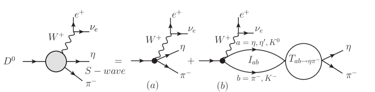
Figure 4: The production mechanism of the four-quark $a_{0}(980)^{-}$ resonance in the decay $D^{0}\to\eta\pi^{-}e^{+}\nu_{e}$.

According to this figure, we write the amplitude $F^{D^{0}}_{d\bar{u}\to S^{-}\to\eta\pi^{-}}(s)$ from Eq. (7) in the form

$$F^{D^{0}}_{d\bar{u}\to S^{-}\to\eta\pi^{-}}(s)=g_{d\bar{u}\eta\pi^{-}}\left[1+I_{\eta\pi^{-}}(s)\,T_{\eta\pi^{-}\to\eta\pi^{-}}(s)\right]+g_{d\bar{u}\eta^{\prime}\pi^{-}}I_{\eta^{\prime}\pi^{-}}(s)\,T_{\eta^{\prime}\pi^{-}\to\eta\pi^{-}}(s)$$

$$+g_{d\bar{u}K^{0}K^{-}}I_{K^{0}K^{-}}(s)\,T_{K^{0}K^{-}\to\eta\pi^{-}}(s),$$ (10)

where $I_{ab}(s)$ is the amplitude of the two-point loop diagram with $ab$ intermediate state and $T_{ab\to\eta\pi^{-}}(s)$ is the amplitude of the $S$-wave $ab\to\eta\pi^{-}$ transition; $ab=\eta\pi^{-},\,\eta^{\prime}\pi^{-},\,K^{0}K^{-}$. The loop amplitude $I_{ab}(s)$ has the form

$$I_{ab}(s)=C_{ab}+\widetilde{I}_{ab}(s)=C_{ab}+\frac{s}{\pi}\int\limits^{\infty}_{m_{ab}^{(+)\,2}}\frac{\rho_{ab}(s^{\prime})\,ds^{\prime}}{\,s^{\prime}(s^{\prime}-s-i\varepsilon)}\,,$$ (11)

where the function $\widetilde{I}_{ab}(s)$ is the singly subtracted at $s=0$ dispersion integral. Explicit expressions for $\widetilde{I}_{ab}(s)$ in different regions of $s$ are given in the Appendix. The real and imaginary parts of this function for different $ab$ are shown in Fig. 5. The quantity $C_{ab}$ in Eq. (11) is a subtraction constant. The choice of these constants will be discussed below.

Figure 5: Line shapes of (a) $\mbox{Re}\widetilde{I}_{ab}(s)$ and (b) $\mbox{Im}\widetilde{I}_{ab}(s)$ for the intermediate states $ab=\eta\pi^{-}$, $K^{0}K^{-}$, and $\eta^{\prime}\pi^{-}$.

We saturate the amplitudes $T_{ab\to\eta\pi^{-}}(s)$ with the contribution of the four-quark $a_{0}(980)^{-}$ resonance. The flavor structure of its wave function has the form Ja77

$$a_{0}(980)^{-}=\bar{u}\bar{s}ds=\frac{1}{\sqrt{2}}\,\eta_{s}\pi^{-}-\frac{1}{\sqrt{2}}\,K^{0}K^{-}.$$ (12)

Considering that $\eta_{s}=s\bar{s}=\eta^{\prime}\sin(\theta_{i}-\theta_{p})-\eta\cos(\theta_{i}-\theta_{p})$, for the coupling constants of the $a_{0}(980)^{-}$ with the superallowed decay channels into pairs of pseudoscalar mesons, the following relations hold:

$$g_{a^{-}_{0}\eta\pi^{-}}=\bar{g}\cos(\theta_{i}-\theta_{p}),\ \ \ g_{a^{-}_{0}\eta^{\prime}\pi^{-}}=-\bar{g}\sin(\theta_{i}-\theta_{p}),\ \ \ g_{a^{-}_{0}K^{0}K^{-}}=\bar{g},$$ (13)

where $\bar{g}$ is the overall coupling constant. Thus,

$$T_{ab\to\eta\pi^{-}}(s)=\frac{g_{a^{-}_{0}ab}g_{a^{-}_{0}\eta\pi^{-}}}{16\pi}\frac{1}{D_{a^{-}_{0}}(s)}\,,$$ (14)

where $D_{a^{-}_{0}}(s)$ is the inverse propagator of the $a_{0}(980)^{-}$ resonance. It has the form

$$D_{a^{-}_{0}}(s)=m^{2}_{a^{-}_{0}}-s+\sum_{ab}[\mbox{Re}\Pi^{ab}_{a^{-}_{0}}(m^{2}_{a^{-}_{0}})-\Pi^{ab}_{a^{-}_{0}}(s)],$$ (15)

where $m_{a^{-}_{0}}$ is the $a_{0}(980)^{-}$ mass and $\Pi^{ab}_{a^{-}_{0}}(s)$ stands for the matrix element of the $a_{0}(980)^{-}$ polarization operator corresponding to the contribution of the $ab$ intermediate state. Re$\Pi^{ab}_{a^{-}_{0}}(s)$ is defined by the singly subtracted at $s=0$ dispersion integral of

$$\mbox{Im}\,\Pi^{ab}_{a^{-}_{0}}(s)=\sqrt{s}\Gamma_{a^{-}_{0}\to ab}(s)=\frac{g^{2}_{a^{-}_{0}ab}}{16\pi}\rho_{ab}(s)\,\theta(\sqrt{s}-m_{a}-m_{b}),$$ (16)

i.e., $\Pi^{ab}_{a^{-}_{0}}(s)=g^{2}_{a^{-}_{0}ab}\,\widetilde{I}_{ab}(s)/(16\pi)$. The terms $\sum_{ab}[\mbox{Re}\Pi^{ab}_{a^{-}_{0}}(m^{2}_{a^{-}_{0}})-\Pi^{ab}_{a^{-}_{0}}(s)]$ in Eq. (15) take into account the finite width corrections and guarantee that the Breit-Wigner mass of the $a_{0}(980)^{-}$ resonance is defined by the condition Re$D_{a^{-}_{0}}(s=m^{2}_{a^{-}_{0}})=0$.

We now rewrite Eq. (III) using Eqs. (9), (13), and (14) and notation $\vartheta=\theta_{i}-\theta_{p}$ as follows:

$$F^{D^{0}}_{d\bar{u}\to S^{-}\to\eta\pi^{-}}(s)=g_{0}\sqrt{2}\sin\vartheta\left[1+\left(I_{\eta\pi^{-}}(s)-I_{\eta^{\prime}\pi^{-}}(s)\right)\frac{\bar{g}^{2}\cos^{2}\vartheta}{16\pi D_{a^{-}_{0}}(s)}\right]+g_{0}I_{K^{0}K^{-}}(s)\frac{\bar{g}^{2}\cos\vartheta}{16\pi D_{a^{-}_{0}}(s)}.$$ (17)

This expression shows that the contributions proportional to the loops $I_{\eta\pi^{-}}(s)$ and $I_{\eta^{\prime}\pi^{-}}(s)$ enter with different signs and therefore partially cancel each other. This cancellation implements the OZI rule in the language of hadronic intermediate states Lip87 ; Lip96 . Indeed, in the case under consideration, the sum of the contributions of the $\eta\pi^{-}$ and $\eta^{\prime}\pi^{-}$ loops is due to the transition $d\bar{u}\to\eta_{n}\pi^{-}$ and then $\eta_{n}\pi^{-}$ into the $\eta_{s}\pi^{-}$ component of the $a_{0}(980)^{-}$ wave function, which is suppressed according to the OZI rule.

Let us discuss the choice of the subtraction constants $C_{ab}$ in the loops $I_{ab}(s)$, see (11). The assumption that all these constants are equal, $C_{\eta\pi^{-}}=C_{\eta^{\prime}\pi^{-}}=C_{K^{0}K^{-}}$, is simplest and most economical in terms of the number of free parameters. Note that nothing changes if we put $C_{\eta\pi^{-}}=C_{\eta^{\prime}\pi^{-}}\neq C_{K^{0}K^{-}}$, since if $C_{\eta\pi^{-}}=C_{\eta^{\prime}\pi^{-}}$, the expression (17) does not depend on their value at all, due to the OZI reduction, and depends only on the parameter $C_{K^{0}K^{-}}$. Below we utilize this choice for $C_{ab}$. In so doing, the model is still quite flexible.

Thus, there are two parameters characterizing the mechanism of the $a_{0}(980)^{-}$ production in $D^{0}\to a_{0}(980)^{-}e^{+}\nu_{e}\to\eta\pi^{-}e^{+}\nu_{e}$ in our model. They are: the product $f^{D^{0}}_{+}(0)g_{0}$, it determines the general normalization of the decay width, and the constant $C_{K^{0}K^{-}}$ which essentially influences on the shape of the $\eta\pi^{-}$ mass spectrum. The actual parameters of the $a_{0}(980)^{-}$ resonance are its mass $m_{a^{-}_{0}}$ and coupling constant $\bar{g}$, see (13).

Figure 6: The Breit-Wigner line shapes of the $a_{0}(980)^{-}$ resonance in $\eta\pi^{-}$, $K^{0}K^{-}$, and $\eta^{\prime}\pi^{-}$ decay channels, see Eq. (18).

Figure 6 shows as a guide the shapes of the Breit-Wigner mass distributions

$$\frac{d\mathcal{B}(a_{0}(980)^{-}\to ab;s)}{d\sqrt{s}}=\frac{2\sqrt{s}}{\pi}\frac{\sqrt{s}\Gamma_{a^{-}_{0}\to ab}(s)}{|D_{a^{-}_{0}}(s)|^{2}}$$ (18)

for the solitary $a_{0}(980)^{-}$ resonance in $\eta\pi^{-}$, $K^{0}K^{-}$, and $\eta^{\prime}\pi^{-}$ decay channels. They are plotted using Eqs. (13), (15), (16), and (18) at $m_{a^{-}_{0}}=0.985$ GeV and $g^{2}_{a^{-}_{0}\eta\pi^{-}}/(16\pi)=0.2$ GeV². Note that the decay width $\Gamma_{a^{-}_{0}\to\eta\pi^{-}}(s)$ calculated by Eq. (16) at $\sqrt{s}=m_{a^{-}_{0}}$ is approximately equal to 132 MeV, while the visible width of the $a_{0}(980)^{-}$ peak at its half-maximum in $\eta\pi^{-}$ channel is $\approx 55$ MeV (see Fig. 6). This narrowing is the consequence of the proximity of $m_{a^{-}_{0}}$ to the $K^{0}K^{-}$ threshold and strong coupling of the $a_{0}(980)^{-}$ to both $\eta\pi^{-}$ and $K^{0}K^{-}$ decay channel Fl76 ; ADS80 .

Recently, the BESIII Collaboration observed in the high-statistics experiment on the decay $\chi_{c1}\to\eta\pi^{+}\pi^{-}$ the impressive peak from $a_{0}(980)$ resonance in the $\eta\pi$ mass spectra BESIII17 . There is a possibility that the $a_{0}(980)$ resonance will manifest itself in the $D\to\eta\pi e^{+}\nu_{e}$ decays in a similar way. Below we discuss the conditions under which such a possibility is realized in our model.

The solid curve in Fig. 7 shows an example of the shape of the $\eta\pi^{-}$ mass spectrum in the decay $D^{0}\to d\bar{u}e^{+}\nu_{e}\to(S^{-}\to\eta\pi^{-})e^{+}\nu_{e}$ with a peak in the region of 1 GeV due to the creation of the $a_{0}(980)^{-}$ resonance. The calculation was done using Eqs. (7), (13), and (17) at the above values of $m_{a^{-}_{0}}$ and $g^{2}_{a^{-}_{0}\eta\pi^{-}}/(16\pi)$ and $C_{K^{0}K^{-}}=0.6$. The value of $C_{K^{0}K^{-}}$ for this example we took to be comparable with the value of Re$\widetilde{I}_{K^{0}K^{-}}(s)$ in the region near the $K^{0}K^{-}$ threshold, see Fig. 5(a). The difference between the solid curves in Figs. 6 and 7 demonstrates the possible influence of the production mechanism on the shape of the $a_{0}(980)^{-}$ peak in the $\eta\pi^{-}$ channel. The dotted curve in Fig. 7 shows the contribution from the last term in Eq. (17) corresponding, according to diagram (b) in Fig. 4, to creation of the $a_{0}(980)^{-}$ resonance via the $K^{0}K^{-}$ intermediate state. The dash-dotted curve shows the contribution due to the seed pointlike diagram (a) in Fig. 4. In Eq. (17), it corresponds to the term equal to $g_{0}\sqrt{2}\sin\vartheta$. The long dashed curve shows the total contribution to the $a_{0}(980)^{-}$ production from the $\eta\pi^{-}$ and $\eta^{\prime}\pi^{-}$ intermediate states (see Fig. 4). In Eq. (17), this contribution is proportional to $\left(I_{\eta\pi^{-}}(s)-I_{\eta^{\prime}\pi^{-}}(s)\right)$. Recall that we consider the case when $C_{\eta\pi^{-}}=C_{\eta^{\prime}\pi^{-}}$. At last, the short dashed curve in Fig. 7 shows the total contribution due to the terms in square brackets in Eq. (17). It is seen that these terms strongly compensate each other in the region $\sqrt{s}\approx m_{a^{-}_{0}}$. First, this happens because in this region Re$\left(\widetilde{I}_{\eta\pi^{-}}(s)-\widetilde{I}_{\eta^{\prime}\pi^{-}}(s)\right)\approx 0$, as shown in Fig. 5(a). Second, the other contributions for $\sqrt{s}<m_{K^{0}}+m_{K^{-}}$ can be represented as $e^{i\delta_{\eta\pi^{-}}(s)}\cos\delta_{\eta\pi^{-}}(s)$, where $\delta_{\eta\pi^{-}}(s)$ is the phase of the $S$-wave elastic $\eta\pi^{-}$ scattering amplitude. In this case, $\delta_{\eta\pi^{-}}(s)$ is a purely resonant phase and therefore $\cos\delta_{\eta\pi^{-}}(m^{2}_{a^{-}_{0}})=0$. Our statement follows from the chain of equalities:

$$1+i\mbox{Im}I_{\eta\pi^{-}}(s)\frac{\bar{g}^{2}\cos^{2}\vartheta}{16\pi D_{a^{-}_{0}}(s)}=1+i\rho_{\eta\pi^{-}}(s)T_{\eta\pi^{-}\to\eta\pi^{-}}(s)=1+i\rho_{\eta\pi^{-}}(s)\frac{e^{2i\delta_{\eta\pi^{-}}(s)}-1}{2\rho_{\eta\pi^{-}}(s)}=e^{i\delta_{\eta\pi^{-}}(s)}\cos\delta_{\eta\pi^{-}}(s).$$

Thus, the phase of the amplitude $F^{D^{0}}_{d\bar{u}\to S^{-}\to\eta\pi^{-}}(s)$, see Eq. (17), for $\sqrt{s}<m_{K^{0}}+m_{K^{-}}$ coincides with the phase of the elastic $\eta\pi^{-}$ scattering in accordance with the requirement of the unitarity condition Wa52 . Equation (III), which has a more general form, also satisfies the unitarity requirement, since in the elastic region the phases of the amplitudes $T_{\eta^{\prime}\pi^{-}\to\eta\pi^{-}}(s)$ and $T_{K^{0}K^{-}\to\eta\pi^{-}}(s)$ coincide with the phase of the amplitude $T_{\eta\pi^{-}\to\eta\pi^{-}}(s)$ and the functions $I_{\eta^{\prime}\pi^{-}}(s)$ and $I_{K^{0}K^{-}}(s)$ are real. The phenomenon of compensation of the pointlike production amplitude [$g_{0}\sqrt{2}\sin\vartheta$ in Eq. (17)] by the resonant one at $\sqrt{s}\approx m_{\mbox{\scriptsize{res}}}$ is also well known, see, for example, Om58 ; GRS69 .

Figure 7: The solid curve shows an example of the shape of the $\eta\pi^{-}$ mass spectrum in the decay $D^{0}\to d\bar{u}e^{+}\nu_{e}\to(S^{-}\to\eta\pi^{-})e^{+}\nu_{e}$ with a peak in the region of 1 GeV due to the creation of the $a_{0}(980)^{-}$ resonance. Detailed description of the components of this spectrum, shown in the figure by other curves, is given in the text. The scale along the ordinate axis is chosen arbitrarily.

The relative role of the $K^{0}K^{-}$ intermediate state in the $a_{0}(980)^{-}$ production increases with increasing the parameter $C_{K^{0}K^{-}}$. The width of the resonance peak in the $\eta\pi^{-}$ mass spectrum narrows, while its height increases and it becomes more pronounced. However, the characteristic enhancement of the left wing of the resonance spectrum and a sharp jump of its right wing (see Fig. 7), caused by interference between different contributions, persist when $C_{K^{0}K^{-}}$ changes over a wide range. The specific form of the $\eta\pi^{-}$ mass spectrum is directly related to the considered mechanism of the $a_{0}(980)^{-}$ production and therefore can serve as its indicator.

Decays of $D^{+}\to a_{0}(980)^{0}e^{+}\nu_{e}\to\eta\pi^{0}e^{+}\nu_{e}$ and $D^{0}\to a_{0}(980)^{-}e^{+}\nu_{e}\to\eta\pi^{-}e^{+}\nu_{e}$ have the same mechanisms, as is clear from Figs. 8, 9 and 3, 4.

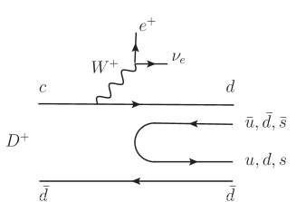
Figure 8: The OZI allowed four-quark fluctuations of the $d\bar{d}$ source, $d\bar{d}\to d\bar{q}q\bar{d}$.

Figure 9: The production mechanism of the four-quark $a_{0}(980)^{0}$ resonance in the decay $D^{+}\to\eta\pi^{0}e^{+}\nu_{e}$.

Their amplitudes $F^{D^{+}}_{d\bar{d}\to S^{0}\to\eta\pi^{0}}(s)$ and $F^{D^{0}}_{d\bar{u}\to S^{-}\to\eta\pi^{-}}(s)$ [see Eq. (17)] are related to each other (within a constant phase factor which can be chosen equal to one) by the relation

$$F^{D^{+}}_{d\bar{d}\to S^{0}\to\eta\pi^{0}}(s)=-\frac{1}{\sqrt{2}}F^{D^{0}}_{d\bar{u}\to S^{-}\to\eta\pi^{-}}(s)$$ (19)

which follows from the assumption of equality of the $a_{0}(980)^{0}$ and $a_{0}(980)^{-}$ masses and isotopic symmetry for the coupling constants. It is easy to check using the following relations

$$g_{d\bar{d}\eta\pi^{0}}=-g_{0}\sin(\theta_{i}-\theta_{p}),\ \ \ g_{d\bar{d}\eta^{\prime}\pi^{-}}=-g_{0}\cos(\theta_{i}-\theta_{p}),\ \ \ g_{d\bar{d}K^{0}\bar{K}0}=g_{0},\qquad\qquad\quad$$ (20)

$$g_{a^{0}_{0}\eta\pi^{0}}=\bar{g}\cos(\theta_{i}-\theta_{p}),\ \ \ g_{a^{0}_{0}\eta^{\prime}\pi^{0}}=-\bar{g}\sin(\theta_{i}-\theta_{p}),\ \ \ g_{a^{0}_{0}K^{+}K^{-}}=\bar{g}/\sqrt{2},\ \ \ g_{a^{0}_{0}K^{0}K^{0}}=-\bar{g}/\sqrt{2},$$ (21)

together with Eqs. (9) and (13). Relations in (21) take into account that the flavor structure of the $a_{0}(980)^{0}$ wave function has the form Ja77

$$a_{0}(980)^{0}=\frac{1}{\sqrt{2}}(u\bar{u}-d\bar{d})s\bar{s}=\frac{1}{\sqrt{2}}\,\eta_{s}\pi^{-}-\frac{1}{{2}}\,K^{+}K^{-}+\frac{1}{{2}}\,K^{0}\bar{K}^{0}.$$ (22)

Of course, for $m_{a_{0}^{-}}=m_{a_{0}^{0}}$ Eq. (19) may be slightly violated in the region of the $K\bar{K}$ thresholds, but the relation for the total decay widths

$$\frac{\Gamma(D^{0}\to\eta\pi^{-}e^{+}\nu_{e})}{\Gamma(D^{+}\to\eta\pi^{0}e^{+}\nu_{e})}=2$$ (23)

should hold very well. However, it should be noted here that the shapes of the $\eta\pi^{-}$ and $\eta\pi^{0}$ mass spectra near the $K\bar{K}$ thresholds are very sensitive to the $a_{0}(980)$ mass and this fact can be used to estimate the mass difference of the $a_{0}(980)^{-}$ and $a_{0}(980)^{0}$ states in the $D$ decays. For example, if $m_{a_{0}^{0}}\approx 0.985$ GeV and $m_{a_{0}^{-}}\approx 0.995$ GeV PDG2020 ; BESIII17 ; Te98 ; Ac17 ; AK18a , then this reduces the ratio (23) by $(5-6)$%.

IV $a_{0}(980)$ resonance in the $D\to K\bar{K}e^{+}\nu_{e}$ decays

Production of the subthreshold $a_{0}(980)^{-}$ resonance in the decay $D^{0}\to K^{0}K^{-}e^{+}\nu_{e}$ is strongly (at least an order of magnitude) suppressed by the phase space in comparison with its production in $D^{0}\to\eta\pi^{-}e^{+}\nu_{e}$. Certainly, experimental investigations of the $D\to K\bar{K}e^{+}\nu_{e}$ decays near the $K\bar{K}$ thresholds is a difficult problem. A detailed theoretical analysis of these decays will be urgent as soon as it becomes possible to carry out the corresponding measurements. Therefore, here we only briefly describe the characteristic features of the $K\bar{K}$ mass spectra associated with the manifestation of the $a_{0}(980)$ resonance in our model.

By analogy with Eq. (17), we write the amplitude for the $D^{0}\to K^{0}K^{-}e^{+}\nu_{e}$ decay in the form

$$F^{D^{0}}_{d\bar{u}\to S^{-}\to K^{0}K^{-}}(s)=g_{0}\left[1+I_{K^{0}K^{-}}(s)\frac{\bar{g}^{2}}{16\pi D_{a^{-}_{0}}(s)}\right]+g_{0}\sqrt{2}\sin\vartheta\cos\vartheta\left(I_{\eta\pi^{-}}(s)-I_{\eta^{\prime}\pi^{-}}(s)\right)\frac{\bar{g}^{2}}{16\pi D_{a^{-}_{0}}(s)}.$$ (24)

The corresponding $K^{0}K^{-}$ mass spectrum is shown in Fig. 10. A feature of this spectrum is the strong destructive interference between the amplitude of the point-like production of $K^{0}K^{-}$ [i.e., $g_{0}$ in Eq. (24)] and the amplitudes containing the contribution from the $a_{0}(980)^{-}$ resonance. As a result, there arises a resonancelike structure in the region $m_{K^{0}}+m_{K^{-}}<\sqrt{s}<1.1$ GeV.

Figure 10: The solid curve shows manifestation of the $a_{0}(980)^{-}$ resonance in the $K^{0}K^{-}$ mass spectrum in the decay $D^{0}\to K^{0}K^{-}e^{+}\nu_{e}$. The dash-dotted curve shows the contribution of the point-like $K^{0}K^{-}$ production amplitude [i.e., $g_{0}$ in Eq. (24)]. The scale along the ordinate axis is the same as in Fig. 7.

The $a_{0}(980)^{0}$ contributions to the amplitudes of the $D^{+}\to K^{0}\bar{K}^{0}e^{+}\nu_{e}$ and $D^{+}\to K^{+}K^{-}e^{+}\nu_{e}$ decays are

$$F^{D^{+}}_{d\bar{d}\to S^{0}\to K^{0}\bar{K}^{0}}(s)=g_{0}\left[1+I_{K^{0}\bar{K}^{0}}(s)\frac{\bar{g}^{2}}{32\pi D_{a^{0}_{0}}(s)}\right]+g_{0}\sin\vartheta\cos\vartheta\left(I_{\eta\pi^{-}}(s)-I_{\eta^{\prime}\pi^{-}}(s)\right)\frac{\bar{g}^{2}}{\sqrt{2}16\pi D_{a^{0}_{0}}(s)},$$ (25)

$$F^{D^{+}}_{d\bar{d}\to S^{0}\to K^{+}K^{-}}(s)=-g_{0}I_{K^{+}K^{-}}(s)\frac{\bar{g}^{2}}{32\pi D_{a^{0}_{0}}(s)}-g_{0}\sin\vartheta\cos\vartheta\left(I_{\eta\pi^{-}}(s)-I_{\eta^{\prime}\pi^{-}}(s)\right)\frac{\bar{g}^{2}}{\sqrt{2}16\pi D_{a^{0}_{0}}(s)}.$$ (26)

The corresponding $K^{0}\bar{K}^{0}$ and $K^{+}K^{-}$ mass spectra are shown in Fig. 11, together with the $K^{0}K^{-}$ one. Here we pay attention to the dominance of the decay channel into $K^{0}\bar{K}^{0}$ over the $K^{+}K^{-}$ channel.

Figure 11: The $K\bar{K}$ mass spectra in the decays $D\to K\bar{K}e^{+}\nu_{e}$ caused by the $a_{0}(980)$ resonance production. The scale along the ordinate axis is the same as in Fig. 7.

In fact, the decays $D^{+}\to K^{0}\bar{K}^{0}e^{+}\nu_{e}$ and $D^{+}\to K^{+}K^{-}e^{+}\nu_{e}$ are more complicated than the decay $D^{0}\to K^{0}K^{-}e^{+}\nu_{e}$, as they can also contain the contribution from the isoscalar $f_{0}(980)$ resonance.

V Conclusion

A simple model of the four-quark mechanism of the $a_{0}(980)$ resonance production in the decays $D^{0}\to\eta\pi^{-}e^{+}\nu_{e}$ and $D^{+}\to\eta\pi^{0}e^{+}\nu_{e}$ is constructed. It is shown that the characteristic features of the shape of the $\eta\pi^{-}$ and $\eta\pi^{0}$ mass spectra can serve as the indicator of the production mechanism and internal structure of the $a_{0}(980)$ state. Future experiments with high statistics on the decays $D\to a_{0}(980)e^{+}\nu_{e}\to\eta\pi e^{+}\nu_{e}$ are highly demanded by the physics of light scalar mesons.

ACKNOWLEDGMENTS

The work was carried out within the framework of the state contract of the Sobolev Institute of Mathematics, Project No. 0314-2019-0021.

APPENDIX:  THE FUNCTION $\widetilde{I}_{ab}(s)$

The dispersion integral $\widetilde{I}_{ab}(s)$ defined in Eq. III is given by: for $s>m_{ab}^{(+)\,2}$

$$\widetilde{I}_{ab}(s)=\frac{s}{\pi}\int\limits^{\infty}_{m_{ab}^{(+)\,2}}\frac{\rho_{ab}(s^{\prime})\,ds^{\prime}}{\,s^{\prime}(s^{\prime}-s-i\varepsilon)}=L_{ab}(s)+\rho_{ab}(s)\left(i-\frac{1}{\pi}\,\ln\frac{\sqrt{s-m_{ab}^{(-)\,2}}+\sqrt{s-m_{ab}^{(+)\,2}}}{\sqrt{s-m_{ab}^{(-)\,2}}-\sqrt{s-m_{ab}^{(+)\,2}}}\right),$$ (A1)

where $m_{ab}^{(\pm)}=m_{a}\pm m_{b}$,  $m_{a}>m_{b}$,  $\rho_{ab}(s)=\sqrt{s-m_{ab}^{(+)\,2}}\,\sqrt{s-m_{ab}^{(-)\,2}}\,/s$,  and

$$L_{ab}(s)=\frac{1}{\pi}\left[1+\left(\frac{m_{ab}^{(+)\,2}+m_{ab}^{(-)\,2}}{2m_{ab}^{(+)}m_{ab}^{(-)}}-\frac{m_{ab}^{(+)}m_{ab}^{(-)}}{s}\right)\ln\frac{m_{a}}{m_{b}}\right];$$

for $m_{ab}^{(-)\,2}<s<m_{ab}^{(+)\,2}$

$$\widetilde{I}_{ab}(s)=L_{ab}(s)-\rho_{ab}(s)\left(1-\frac{2}{\pi}\arctan\frac{\sqrt{m_{ab}^{(+)\,2}-s}}{\sqrt{s-m_{ab}^{(-)\,2}}}\right),$$ (A2)

where $\rho_{ab}(s)$ = $\sqrt{m_{ab}^{(+)\,2}-s}\,\sqrt{s-m_{ab}^{(-)\,2}}\,/s$;  and for $s<m_{ab}^{(-)\,2}$

$$\widetilde{I}_{ab}(s)=L_{ab}(s)+\frac{\rho_{ab}(s)}{\pi}\,\ln\frac{\sqrt{m_{ab}^{(+)\,2}-s}+\sqrt{m_{ab}^{(-)\,2}-s}}{\sqrt{m_{ab}^{(+)\,2}-s}-\sqrt{m_{ab}^{(-)\,2}-s}},$$ (A3)

where $\rho_{ab}(s)$ = $\sqrt{m_{ab}^{(+)\,2}-s}\,\sqrt{m_{ab}^{(-)\,2}-s}\,/s$. If $b=\bar{a}$, then $m_{b}=m_{a}$ and $\widetilde{I}_{ab}(s)=\widetilde{I}_{a\bar{a}}(s)$ has a more simple form:

$$\widetilde{I}_{a\bar{a}}(s) = \frac{2}{\pi}+\rho_{a\bar{a}}(s)\left(i-\frac{1}{\pi}\,\ln\frac{1+\rho_{a\bar{a}}(s)}{1-\rho_{a\bar{a}}(s)}\right),\quad\mbox{for }s>4m^{2}_{a},\ \ \mbox{ and}$$ (A4)

$$\widetilde{I}_{a\bar{a}}(s) = \frac{2}{\pi}-|\rho_{a\bar{a}}(s)|\left(1-\frac{2}{\pi}\,\arctan|\rho_{a\bar{a}}(s)|\right),\quad\mbox{for }0<s<4m^{2}_{a},$$ (A5)

where $\rho_{a\bar{a}}(s)=\sqrt{1-4m^{2}_{a}/s}\,$.

References

(1) K. M. Ecklund et al. (CLEO Collaboration), Phys. Rev. D 80, 052009 (2009).
(2) W. Wang and C. D. Lü, Phys. Rev. D 82, 034016 (2010).
(3) M. R. Pennington, AIP Conf. Proc. 1257, 27 (2010).
(4) A. H. Fariborz, R. Jora, J. Schechter, and M. N. Shahid, Phys. Rev. D 84, 094024 (2011).
(5) N. N. Achasov and A. V. Kiselev, Phys. Rev. D 86, 114010 (2012).
(6) P. A. Zyla et al. (Particle Data Group), Prog. Theor. Exp. Phys. 2020, 083C01 (2020).
(7) B. Aubert et al. (BABAR Collaboration), Phys. Rev. D 78, 051101(R) (2008).
(8) J. Yelton et al. (CLEO Collaboration), Phys. Rev. D 80, 052007 (2009).
(9) M. Ablikim et al. (BESIII Collaboration), Phys. Rev. Lett. 121, 081802 (2018).
(10) M. Ablikim et al. (BESIII Collaboration), Phys. Rev. Lett. 122, 062001 (2019).
(11) M. Ablikim et al. (BESIII Collaboration), Phys. Rev. D 103, 092004 (2021).
(12) N. N. Achasov and A. V. Kiselev, Int. J. Mod. Phys. Conf. Ser. 35, 1460447 (2014).
(13) T. Sekihara and E. Oset, Phys. Rev. D 92, 054038 (2015).
(14) Y. J. Shi, W. Wang, and S. Zhao, Eur. Phys. J. C 77, 452 (2017).
(15) X. D. Cheng, H. B. Li, B. Wei, Y. G. Xu, and M. Z. Yang, Phys. Rev. D 96, 033002 (2017).
(16) N. N. Achasov and A. V. Kiselev, Phys. Rev. D 98, 096009 (2018).
(17) N. N. Achasov and A. V. Kiselev, EPJ Web Conf. 212, 03001 (2019).
(18) N. N. Achasov, Phys. Part. Nucl., 51, 632 (2020).
(19) N. R. Soni, A. N. Gadaria, J. J. Patel, and J. N. Pandya, Phys. Rev. D 102, 016013 (2020).
(20)N. N. Achasov, A. V. Kiselev, and G. N. Shestakov, Phys. Rev. D 102, 016022 (2020).
(21)Y. J. Shi, C. Y. Seng, F. K. Guo, B. Kubis, U.-G. Meißner, and W. Wang, J. High Energy Phys. 04 (2021) 086.
(22)Y. J. Shi and U.-G. Meißner, Eur. Phys. J. C 81, 412 (2021).
(23) R. L. Jaffe, Phys. Rev. D 15, 267 (1977); 15, 281 (1977).
(24) N. N. Achasov and V. N. Ivanchenko, Nucl. Phys. B315, 465 (1989).
(25) N. N. Achasov, J. V. Bennett, A. V. Kiselev, E. A. Kozyrev, and G. N. Shestakov, Phys. Rev. D 103, 014010 (2021).
(26) M. Ablikim et al. (BESIII Collaboration), Phys. Rev. D 92, 052003 (2015).
(27) R. M. Baltrusaitis et al. (MARK III Collaboration), Phys. Rev. Lett. 56, 2140 (1986).
(28) P. del Amo Sanchez et al. (BABAR Collaboration), Phys. Rev. D 83, 072001 (2011).
(29) S. Okubo, Phys. Lett. 5, 165 (1963).
(30) S. Okubo, Progr. Theor. Phys. 63, 1 (1978).
(31) G. Zweig, in Developments in the Quark Theory of Hadrons, edited by D.B. Lichtenberg and S.P.
Rosen (Hadronic Press, Massachusetts, 1980).
(32) J. Iizuka, Prog. Theor. Phys. Suppl. 37, 21 (1966).
(33)H. J. Lipkin, Nucl. Phys. B291, 720 (1987).
(34)H. J. Lipkin and B. S. Zou, Phys. Rev. D 53, 6693 (1996).
(35) S. M. Flatte, Phys. Lett. 63B, 224 (1976).
(36)N. N. Achasov, S. A. Devyanin, and G. N. Shestakov, Phys. Lett. 96B, 168 (1980).
(37)M. Ablikim et al. (BESIII Collaboration), Phys. Rev. D 95, 032002 (2017).
(38) K. M. Watson, Phys. Rev. 88, 1163 (1952).
(39) R. Omnès, Nuovo Cimento A 8, 316 (1958).
(40)M. Gourdin, F.M. Renard, and L. Stodolsky, Phys. Lett. 30B, 347 (1969).
(41) S. Teige et al. (E852 Collaboration), Phys. Rev. D 59, 012001 (1998).
(42) S. Acharya et al. (ALICE Collaboration), Phys. Lett. B 774, 64 (2017).
(43)N. N. Achasov and A. V. Kiselev, Phys. Rev. D 97, 036015 (2018).