NoiseGrad — Enhancing Explanations
by Introducing Stochasticity to Model Weights

Abstract

Many efforts have been made for revealing the decision-making process of black-box learning machines such as deep neural networks, resulting in useful local and global explanation methods. For local explanation, stochasticity is known to help: a simple method, called SmoothGrad, has improved the visual quality of gradient-based attribution by adding noise to the input space and averaging the explanations of the noisy inputs. In this paper, we extend this idea and propose NoiseGrad that enhances both local and global explanation methods. Specifically, NoiseGrad introduces stochasticity in the weight parameter space, such that the decision boundary is perturbed. NoiseGrad is expected to enhance the local explanation, similarly to SmoothGrad, due to the dual relationship between the input perturbation and the decision boundary perturbation. We evaluate NoiseGrad and its fusion with SmoothGrad — FusionGrad — qualitatively and quantitatively with several evaluation criteria, and show that our novel approach significantly outperforms the baseline methods. Both NoiseGrad and FusionGrad are method-agnostic and as handy as SmoothGrad using a simple heuristic for the choice of the hyperparameter setting without the need of fine-tuning.

Introduction

The ubiquitous usage of Deep Neural Networks (DNNs), fueled by their ability to generalize and learn complex nonlinear functions, has presented both researchers and practitioners with the problem of non-interpretability and opaqueness of Machine Learning (ML) models. This lack of transparency, coupled with the widespread use of these highly complex models in practice, represents a risk and a major challenge for the responsible usage of artificial intelligence, especially in security-critical areas, e.g. the medical field. In response to this, the field of eXplainable AI (XAI) has emerged intending to make the predictions of complex algorithms comprehensible for humans.

One possible dichotomy of post-hoc explanation methods can be carried out on the basis of whether these methods refer to the global or local properties of a learning machine. The local level XAI aims to explain a model decision of an individual input (Guidotti et al. 2018), for which various methods, such as Layer-wise Relevance Propagation (LRP) (Bach et al. 2015b), GradCAM (Selvaraju et al. 2019), Occlusion (Zeiler and Fergus 2014), MFI (Vidovic et al. 2016), Integrated Gradient (Sundararajan, Taly, and Yan 2017), have proven effective in explaining DNNs. In contrast, global explanations aim to illustrate the decision process as a whole, without the connection to individual data samples. Recently, methods belonging to the Activation-Maximization (Erhan et al. 2009) family of methods have become widely popular, such as DeepDream (Mordvintsev, Olah, and Tyka 2015), GAN-generated explanations (Nguyen et al. 2016) and Feature Visualization (Olah, Mordvintsev, and Schubert 2017).

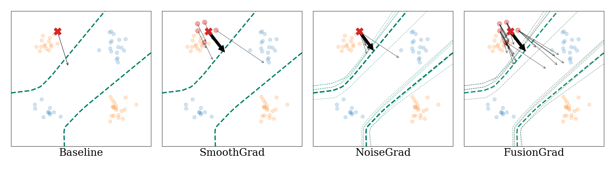
Figure 1: Illustration of the differences in explanation behavior between Baseline (gradient-based explanation), SmoothGrad, NoiseGrad, and FusionGrad for a toy experiment. Given training samples of two classes (orange and blue dots), a 3-layer MLP was trained for binary classification, where the learned decision boundary is shown by the green dashed line. The gradient explanations for a fixed test sample (red point) are shown as black arrows and the mean explanation as a bold black arrow. (a) For the baseline method, the explanation is the gradient itself. (b) SmoothGrad enhances the explanation by sampling points in the neighborhood (small red dots), and averaging their explanations (bold black arrow). (c) NoiseGrad enhances the explanation by averaging over perturbed models, indicated by multiple decision boundaries (thin green dashed lines). (d) FusionGrad combines SmoothGrad and NoiseGrad by incorporating both stochasticities in the input space and the model space.

For local explanation, gradient-based methods are most popular due to their simplicity, however, they tend to suffer from the gradient shattering effect, which often results in noisy explanation maps (Samek et al. 2021). As a remedy, Smilkov et. al. proposed a simple method, called SmoothGrad (Smilkov et al. 2017), where stochasticity is introduced to the input. Specifically, it adds Gaussian Noise to the input features $n$ times, computes the $n$ corresponding explanations, and takes the average over the $n$ explanations. SmoothGrad is applicable to any local explanation method and has been practically proven to reduce the visual noise in the explanation map.

The mechanism behind SmoothGrad’s enhancement of explanations is not yet well understood. One could argue that SmoothGrad averages out the shattering effect. However, SmoothGrad performs best when the added noise level is around 10%–20% of the signal level, which not only smooths out peaky derivatives but is large enough to cross the decision boundary. From this fact, we hypothesize that SmoothGrad perturbs the test sample in order to get a signal from the steepest part of the decision boundary. This motivated us to explore another way of using stochasticity: instead of adding noise to the input, our proposed method — NoiseGrad (NG) — draws samples from the network weights from a tempered Bayes posterior (Wenzel et al. 2020), such that the decision boundaries of some models are close to the test sample, which results in more precise explanations.

Our hypothesis leads to a natural and easy way of hyperparameter choice: the noise level added to the weights (which corresponds to the temperature of the tempered Bayes posterior) is chosen such that the relative performance drop is around $5\%$. In addition, we approximate the tempered Bayes posterior by multiplicative noise applied to the network weights — in the same spirit as MC dropout (Gal and Ghahramani 2016). Thus, our proposed method NoiseGrad can be implemented as easily as SmoothGrad with an automatic hyperparameter choice and is applicable to any model architecture and explanation method. Our experiments empirically support our hypothesis and show quantitatively and qualitatively that NoiseGrad outperforms SmoothGrad and combining NoiseGrad with SmoothGrad, which we refer to as FusionGrad, further boosts the performance. An overview of our proposed methods is shown on a toy experiment in Figure 1.

Another advantage of NoiseGrad over SmoothGrad is that it is straightforwardly applicable to global explanations as well. For example, we can replace the objective function for activation maximization with its average over the model samples, which is expected to stabilize the image representing the features captured by neurons. Our experiments demonstrate that NoiseGrad improves global explanations in terms of human interpretability and vividness of illustrated abstractions.

Our main contributions include:

• We propose a novel method, NoiseGrad, that improves local and global explanation methods by introducing stochasticity to the model parameters.

• The performance gain by NoiseGrad and its fusion with SmoothGrad, FusionGrad, for local explanations, is shown qualitatively and quantitatively using different evaluation criteria.

• We observe that NoiseGrad is further capable of enhancing global explanation methods.

Background

Let $f(\cdot;\hat{W}):\mathbb{R}^{d}\rightarrow\mathbb{R}^{k}$ be a neural network with learned weights $\hat{W}\subset\mathbb{R}^{S}$ that maps a vector $\boldsymbol{x}\in\mathbb{R}^{d}$ from the input domain to a vector $y\in\mathbb{R}^{k}$ in the output domain. In general, attribution methods could be viewed as an operator $E\left(\boldsymbol{x},f(\cdot,\hat{W})\right)$ that attributes relevances to the features of the input $\boldsymbol{x}$ with respect to the model function $f(\cdot,W)$. More in-depth discussion about the different explanation methods used can be found in the Appendix.

Enhancing local explanations by adding noise to the inputs

A recently proposed popular method, called SmoothGrad (SG), seeks to alleviate noise and visual diffusion of saliency maps by introducing stochasticity to the inputs (Smilkov et al. 2017). SmoothGrad adds Gaussian noise to the input and takes the average over $N$ instances of noise:

$$\begin{split}E_{SG}\left(\boldsymbol{x}\right)=\textstyle\frac{1}{N}\sum_{i=1}^{N}E\left(\boldsymbol{x}+\xi_{i},f(\cdot,\hat{W})\right),\\ \xi_{i}\sim\mathcal{N}(\mathbf{0},\sigma_{\mathrm{SG}}^{2}\mathbf{I})\end{split}$$ (1)

where $\mathcal{N}(\mathbf{\mu},\mathbf{\Sigma})$ is the Normal distribution with mean $\mathbf{\mu}$ and covariance $\mathbf{\Sigma}$ and $\mathbf{I}$ the identity matrix. The authors of the original paper state that SG allows smoothening the gradient landscape, thus providing better explanations. Later SmoothGrad has also proven to be more robust against adversarial attacks (Dombrowski et al. 2019).

Enhancing explanations by approximate Bayesian learning

From a statistical perspective, training DNNs with the most commonly used loss functions and regularizers, such as categorical cross-entropy for classification and MSE for regression, can be seen as performing maximum a-posteriori (MAP) learning. Hence, the resulting weights can be thought of as a point estimate for a posterior mode in the parameter space, capturing no uncertainty information. Recently, Bykov et al. (2021) showed that incorporating information about posterior distribution can enhance local explanations for DNNs. Intuitively, in contrast to the MAP learning, where point estimates of weights represent one deterministic decision-making strategy, a posterior distribution represents an infinite ensemble of models, which employ different strategies towards the prediction. By aggregating the variability of the decision-making processes of networks, we can obtain a broader outlook on the features that were used for the prediction, and thus deeper insights into the models’ behavior (Grinwald et al. 2022).

Since exact Bayesian Learning is intractable for DNNs, a plethora of approximation methods have been proposed, e.g., Laplace Approximation (Ritter, Botev, and Barber 2018), Variational Inference (Graves 2011; Osawa et al. 2019), MC dropout (Gal and Ghahramani 2016), Variational Dropout (Kingma, Salimans, and Welling 2015; Molchanov, Ashukha, and Vetrov 2017), MCMC sampling (Wenzel et al. 2020). Since most of the approximation methods require full retraining of the network or evaluation of the second-order statistics, which are computationally expensive, we use a cruder approximation with multiplicative noise to draw model samples for NoiseGrad.

Method

As mentioned previously, the mechanism why SmoothGrad improves explanations has not been well understood. In empirical experiments we found that SmoothGrad with a recommended 10%–20% noise level is large enough to cross the decision boundary, resulting in a significant classification accuracy drop. This finding implies that SmoothGrad does not only smooth the peaky derivative but also collects signals from the steepest part of the likelihood, i.e., decision boundary, by perturbing the input sample with large noise.

Motivated by this observation, we propose another way of introducing stochasticity – instead of perturbing the input, we perturb the model itself. More specifically, we propose a new method — NoiseGrad — which draws network weight samples from a tempered Bayes posterior (Wenzel et al. 2020), i.e., the Bayes posterior with a temperature higher than 1. The temperature should be so high that the decision boundaries of some model samples are close to the test sample, which reinforces the signals for explanations.

Local explanation with NoiseGrad

Mathematically, we define the local explanation with NoiseGrad (NG) as follows

$$E_{\mathrm{NG}}(\boldsymbol{x})=\textstyle\frac{1}{M}\sum_{i=1}^{M}E\left(\boldsymbol{x},f(\cdot,\mathcal{W}_{i})\right),$$ (2)

where $\{\mathcal{W}_{i}\},i\in[1,M]$ are samples drawn from a tempered Bayes posterior. Since approximate Bayesian learning is computationally expensive, we approximate the posterior with multiplicative Gaussian noise – in the spirit of MC dropout (Gal and Ghahramani 2016): $\mathcal{W}_{i}=\hat{W}\cdot\eta_{i},$ with $\eta_{i}\sim\mathcal{N}(\mathbf{1},\,\sigma_{\mathrm{NG}}^{2}\mathbf{I})$, where $\mathbf{I}$ refers to an identity matrix. By averaging over a sufficiently large number of samples $M$, we expect NG to smooth the signal and also to collect amplified signals from models whose decision boundary is close to the test sample. This and the smoothing capabilities of the NG method can be observed in Figure 2, where the gradients are plotted for each grid-point on the toy dataset used before in Figure 1 for both Baseline and NG. From the results shown, we can observe that NoiseGrad in fact smoothens out the gradient.

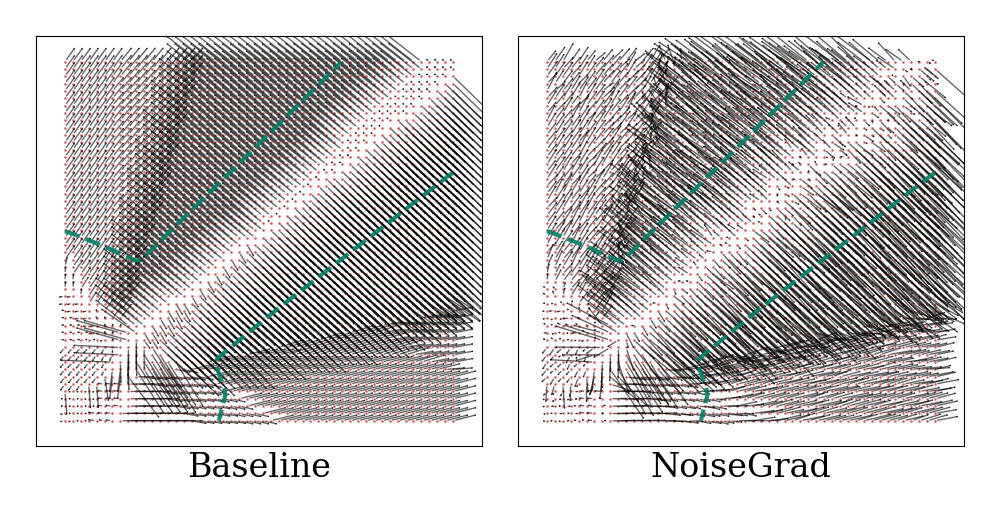
Figure 2: Illustration of the impact of NoiseGrad on a gradient flow map. For the same problem as in Figure 1, for each grid-point the gradient is computed (left). On the right we can observe the effect of NoiseGrad — it smoothens the gradients by perturbing the decision boundary.

FusionGrad

We also propose FusionGrad (FG), a combination of NoiseGrad and SmoothGrad, to incorporate both stochasticities in the input space and the model space

$$E_{\mathrm{FG}}(\boldsymbol{x})=\textstyle\frac{1}{N}\sum_{i=1}^{N}\frac{1}{M}\sum_{j=1}^{M}E\left(\boldsymbol{x}+\xi_{j},f(\cdot,\mathcal{W}_{i})\right)$$ (3)

where $\xi_{j}\sim\mathcal{N}(\mathbf{0},\,\sigma_{\mathrm{SG}}^{2}\mathbf{I})$, $N$ the number of noisy inputs, and $M$ the number of model samples. We show in our experiments that FG further boosts the performance of NG, providing the best qualitative and quantitative performances.

Global explanation with NoiseGrad

Unlike SmoothGrad, NoiseGrad can be used to enhance global explanation methods. An important class of global explanation methods is activation maximization (AM) (Erhan et al. 2009), which synthetically creates an input that maximizes a given function $g(x)$. Usually, the activation of a particular neuron is maximized, and thus the generated input can embody the main concepts and abstractions that the DNN is looking for. Many variants with different types of regularization have emerged (Nguyen et al. 2016; Olah, Mordvintsev, and Schubert 2017) — regularization is necessary because otherwise, AM might synthesize adversarial inputs, which would not convey visual information to the investigator.

NoiseGrad enhancement of any AM technique could be performed as follows: given the target function $g(x,\hat{W})$ for a model $f(\cdot;\hat{W})$, we sample $M$ models with the NG procedure, and maximize the average function over the number of perturbed models:

$$\textstyle\operatorname*{arg\,max}_{x\in\mathcal{C}}\frac{1}{M}\sum_{i=1}^{M}g(x,\mathcal{W}_{i}),$$ (4)

where $\mathcal{C}$ is a regularized input domain, specific to a particular implementation of an AM method.

Heuristic for hyperparameter setting

One of the reasons for the popularity of SmoothGrad is that it does not require hyperparameter tuning: it works well if the number $N$ of noisy samples is sufficiently large, and the input noise level $\sigma_{\mathrm{SG}}$ is set to a value in the recommended range, 10%–20%, compared to the signal level.

A major question is if one can set the noise level $\sigma_{\mathrm{NG}}$ for NoiseGrad in a similar way that does not require fine-tuning. We put forward a simple hypothesis: since we need signals from models whose decision boundaries are close to the test sample, we might choose the noise level $\sigma_{\mathrm{NG}}$ such that we observe a certain performance drop. For the classification setting with balanced classes, we can use accuracy as a performance measure: from experimental results (discussed more in-depth in the Appendix) we recommend to set the relative accuracy drop $\textrm{AD}(\sigma)=1-(\textrm{ACC}(\sigma)-\textrm{ACC}(\infty))/(\textrm{ACC}(0)-\textrm{ACC}(\infty))$ to around $5\%$, where $\textrm{ACC}(\sigma)$ denotes the classification accuracy at the noise level $\sigma$. Note that $\textrm{ACC}(0)$ and $\textrm{ACC}(\infty)$ correspond to the original accuracy and the chance level, respectively. This rule of thumb can be used for various model architectures with different scales, as shown in the next section.

As a heuristic for FusionGrad, we recommend to half both $\sigma_{\mathrm{SG}}$ and $\sigma_{\mathrm{NG}}$ (as found by their respective heuristics) to equal the contribution from the input perturbation and the model perturbation. Further, we empirically found that $10$ samples are sufficient for both methods. With those heuristics, NoiseGrad and FusionGrad can be used as effortlessly as SmoothGrad. A detailed discussion on the relationship between the explanation quality (localization criteria) and accuracy drop can be found in the Appendix.

Method	Localization ($\uparrow$)	Faithfulness ($\uparrow$)	Robustness ($\downarrow$)	Sparseness ($\uparrow$)
Baseline	0.7315 $\pm$ 0.0505	0.3413 $\pm$ 0.1549	0.0763 $\pm$ 0.0265	0.6272 $\pm$ 0.0475
SG	0.8263 $\pm$ 0.0483	0.3465 $\pm$ 0.1601	0.0590 $\pm$ 0.0235	0.5310 $\pm$ 0.0635
NG	0.8349 $\pm$ 0.0367	0.3635 $\pm$ 0.1536	0.0224 $\pm$ 0.0080	0.5794 $\pm$ 0.0533
FG	0.8435 $\pm$ 0.0358	0.3697 $\pm$ 0.1465	0.0153 $\pm$ 0.0058	0.5721 $\pm$ 0.0532

Table 1: Comparison of attribution quality where the noise levels are set by the heuristic. $\uparrow$ and $\downarrow$ indicate the larger is the better and the smaller is the better, respectively. The values of the best method and the methods that are not significantly outperformed by the best method, according to the Wilcoxon signed-rank test for $p=0.05$, are bold-faced.

Method	LeNet	VGG11	VGG16	RN9	RN18	RN50
Baseline	0.922 $\pm$ 0.033	0.961 $\pm$ 0.017	0.967 $\pm$ 0.015	0.926 $\pm$ 0.026	0.913 $\pm$ 0.04	0.912 $\pm$ 0.035
SG	0.940 $\pm$ 0.048	0.971 $\pm$ 0.025	0.963 $\pm$ 0.034	0.975 $\pm$ 0.015	0.962 $\pm$ 0.026	0.967 $\pm$ 0.022
NG	0.949 $\pm$ 0.029	0.982 $\pm$ 0.011	0.985 $\pm$ 0.011	0.978 $\pm$ 0.012	0.963 $\pm$ 0.023	0.973 $\pm$ 0.017
FG	0.961 $\pm$ 0.025	0.984 $\pm$ 0.011	0.982 $\pm$ 0.013	0.982 $\pm$ 0.011	0.975 $\pm$ 0.016	0.969 $\pm$ 0.019

Table 2: Attribution ranking scores ($\mathrm{AUC}$) for different architectures with noise levels set by our proposed heuristic. We can observe that either NG or FG outperforms Baseline and SG. For the sake of space, we refer ResNets as RNs.

Experiments On Local Explanations

In this section, we explain datasets and evaluation metrics used for evaluating our proposed methods for local attribution quality.

Datasets

To measure the goodness of an explanation, one typically needs to resort to proxies for evaluation since no ground-truth for explanations exists. Similar to Arras, Osman, and Samek (2020) and Yang and Kim (2019); Romijnders (2017), we therefore design a controlled setting for which the ground-truth segmentation labels are simulated. For this purpose, we construct a semi-natural dataset CMNIST (customized-MNIST), where each MNIST digit (LeCun, Cortes, and Burges 2010) is displayed on a randomly selected CIFAR background (Krizhevsky, Hinton et al. 2009). To ensure that the explainable evidence for a class lies in the vicinity of the object itself, rather than in its contextual surrounding, we uniformly distribute CIFAR backgrounds for each MNIST digit class as we construct the CMNIST dataset. Ground-truth segmentation labels for the explanations are formed by creating different variations of segmentation masks around the object of interest such as a squared box around the object or the pixels of the object itself. Moreover, to understand the real impact of SOTA, we use the PASCAL VOC 2012 object recognition dataset (Everingham et al. 2010) and ILSVRC-15 dataset (Russakovsky et al. 2015) for evaluation, where object segmentation masks in the forms of bounding boxes are available. Further details on training- and test splits, preprocessing steps and other relevant dataset statistics can be found in the Appendix.

In an explainability context, the question naturally arises whether object localization masks can be used as ground-truth labels for explanations of natural datasets in which the independence of the models from the background cannot be guaranteed. We, therefore, report quantitative metrics only on the controlled semi-natural dataset but report qualitative results on the natural dataset as well.

Evaluation metrics

While the debate of what properties an attribution-based explanation ought to fulfill continues, several works (Montavon, Samek, and Müller 2018; Alvarez Melis and Jaakkola 2018; Carvalho, Pereira, and Cardoso 2019) suggest that in order to produce human-meaningful explanations one metric alone is not sufficient. To broaden the view of what it means to provide a good explanation, we evaluate the explanation-enhancing methods using four well-studied properties — localization (Zhang et al. 2018; Kohlbrenner et al. 2020; Theiner, Müller-Budack, and Ewerth 2021; Arras, Osman, and Samek 2020), faithfulness (Bach et al. 2015b; Samek et al. 2016; Bhatt, Weller, and Moura 2020; Nguyen and Martínez 2020; Rieger and Hansen 2020), robustness (Alvarez Melis and Jaakkola 2018; Montavon, Samek, and Müller 2018; Yeh et al. 2019), and sparseness (Nguyen and Martínez 2020; Chalasani et al. 2020; Bhatt, Weller, and Moura 2020). While there exists several empirical interpretations, or operationalizations, for each of these qualities, we selected one metric per category. We adopted Relevance Rank Accuracy (Arras, Osman, and Samek 2020) to express localization of the attributions, Faithfulness correlation (Bhatt, Weller, and Moura 2020) to capture attribution faithfulness, applied max-Sensitivity (Yeh et al. 2019) to express attribution robustness and Gini index (Chalasani et al. 2020) to assess the sparsity of the attributions. All evaluation measures are clearly motivated, defined, and discussed in the Appendix.

Explanation methods

NoiseGrad is method-agnostic, which means, that it can be applied in conjunction with any explanation method. However, in these experiments, we focus on a popular category of post-hoc gradient-based attribution methods and use Saliency (SA) (Mørch et al. 1995) as the base explanation method in the experiments similar as in (Smilkov et al. 2017). Since the majority of model-aware local explanation methods make use of the model gradients, we argue that a potential explanation improvement on SA with our proposed method may also be transferred to an improvement of a related gradient-based explanation method. As the comparative baseline explanation method (Baseline), we employ the Saliency explanation, which adds no noise to either the weights nor the input. We report results on additional explanation methods in the Appendix.

Model architectures

Explanations were produced for networks of different architectural compositions such as ResNet (He et al. 2016), VGG (Simonyan and Zisserman 2014) and LeNet (LeCun et al. 1998). All networks were trained for image classification tasks so that they showcased a comparable test accuracy to a minimum of $86$%, $92$% and $86$% classification accuracy for CMNIST, PASCAL VOC 2012, and ILSVRC-15 datasets respectively. For more details on the model architectures, optimization configurations, and training results, we refer to the Appendix.

Results

In the following, we present our experimental results. The findings can be summarized as follows: (i) both NG and FG offer an advantage over SG measured with several metrics of attribution quality and (ii) as a heuristic, choosing the hyperparameters for NG and FG according to a classification performance drop of 5% typically result in explanations with a high attribution quality.

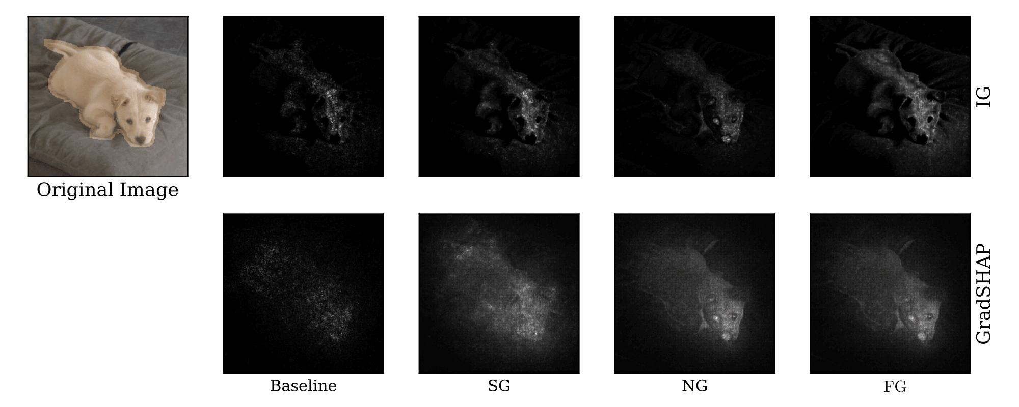
Figure 3: Attribution maps by Baseline, SG, NG, and FG for two base explanation methods Integrated Gradients (IG) and GradientSHAP (GradSHAP), for an image from the PASCAL VOC 2012 dataset. We can observe that both NG and FG improve the sharpness of the attributions compared to Baseline and SG. Moreover, NG highlights semantic features of the dog, such as the nose and the eyes, which are not visible for Baseline and SG.

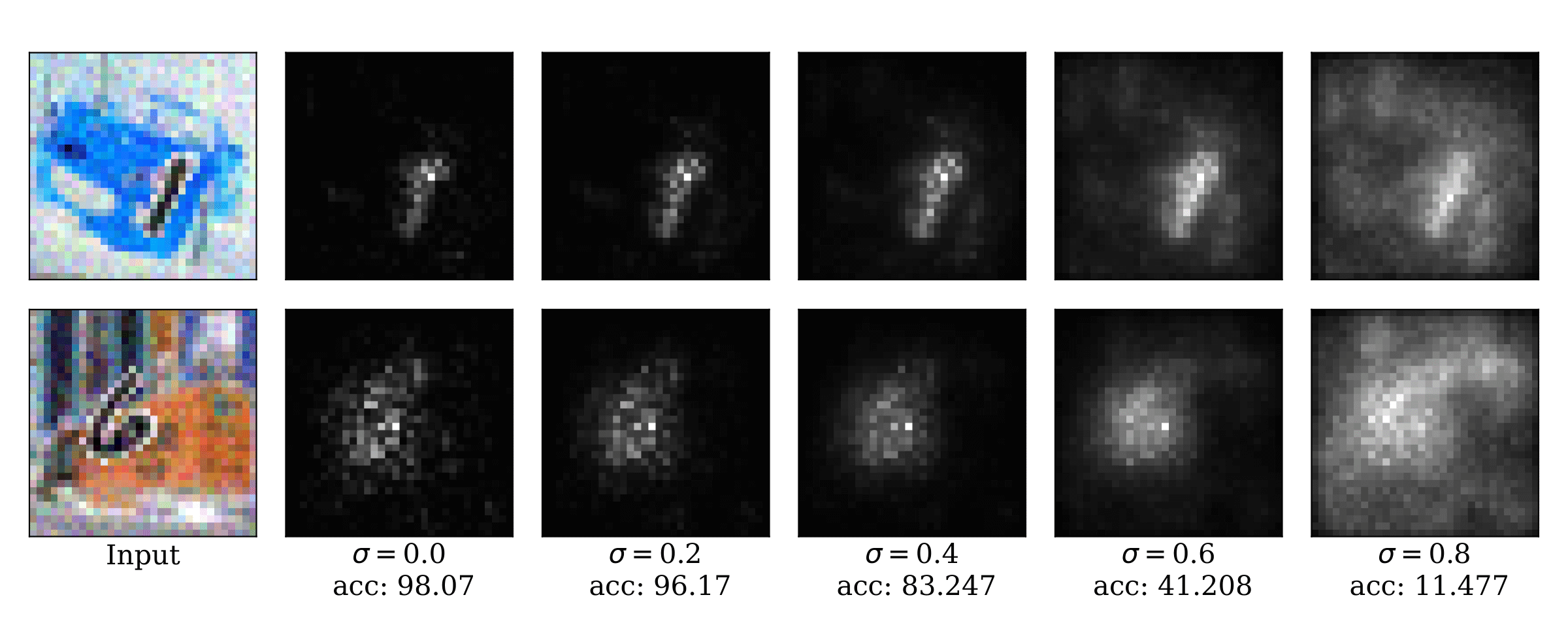
Figure 4: Illustration of NG-enhanced Saliency explanations for the CMNIST dataset: we observe an improvement of the localization ability of the explanation when increasing the hyperparameter $\sigma$ until $\sigma\leq 0.4$ –– afterward, if the noise amplitude becomes too large, the models lose their predicting ability, which results in noisy attribution maps.

Quantitative evaluation

We start by examining the performance of the methods considering the four aforementioned attribution quality criteria applied to the absolute values of their respective explanations. The results are summarized in Table 1, where the methods (Baseline, SG, NG, FG) are stated in the first column and the respective values for localization, faithfulness robustness, and sparseness in columns 2-5. The scores were computed and averaged over 256 randomly chosen test samples from the CMNIST dataset, using a ResNet-9 classifier and the Saliency as the base attribution method. The Quantus library was employed for XAI evaluation (Hedström et al. 2022).

The noise level for SG, NG, and FG is set by the heuristic, which was described in the method section. We conducted the same experiment with additional base attribution methods and datasets and found similar tendencies, which are reported in the Appendix. In the Appendix, we also investigated how the different noise levels for FusionGrad ($\sigma_{\mathrm{NG}}$ and $\sigma_{\mathrm{SG}}$) influence the ranking of attributions, as well as performed model parameter randomization sanity checks (Adebayo et al. 2018).

From Table 1, we can observe a significant attribution quality boost by our proposed methods, NG, and FG in comparison to the baselines, Baseline and SG. For each of the examined quality criteria, the values range between $[0,1]$. For localization, faithfulness, and sparseness higher values are better and for robustness lower values are better. The combination of SmooothGrad and NoiseGrad, i.e., FusionGrad is significantly better than either method alone. In summary, we conclude that NG outperforms SG on all four criteria and Baseline on the most criteria except Sparseness, and FG further boosts the performance. In general, any perturbation naturally degrades the sparseness, and therefore Baseline gives the best sparseness score. Note that NG and FG both improve the other criteria with less degradation of sparseness in comparison to SG. It is important to also emphasize that evaluation of explanation methods should always be viewed holistically — i.e., while Baseline may be the most sparse explanation, it would not be the overall preferred option since it is the least faithful, localized, and robust explanation of them all. Further evaluation results on the ILSVRC-15 dataset can be found in the Appendix.

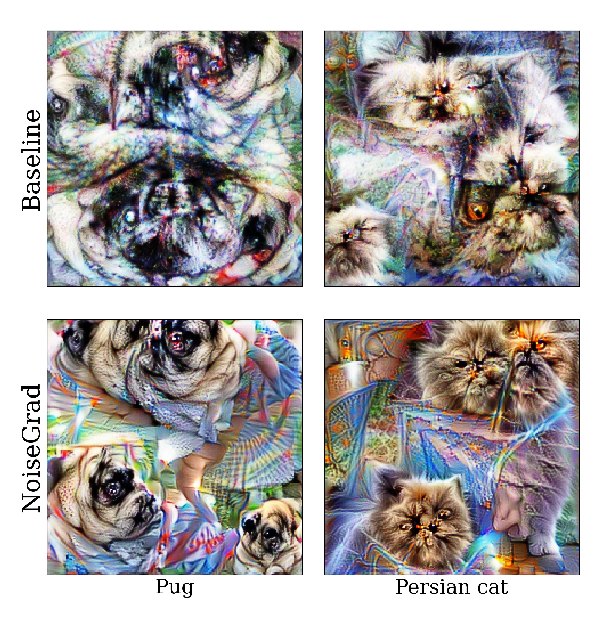
Figure 5: Global explanation by activation maximization (AM) without (top row) and with (bottom) NoiseGrad, applied to ResNet-18 network pre-trained on ImageNet dataset. For each column, the output neuron for the specified class is explained.

Heuristic applied to different architectures

In Table 2, we present ranking $\mathrm{AUC}$ scores for different model architectures trained on CMNIST, using the recommended heuristic to set the noise level.

We can observe that appropriate noise levels are chosen with the proposed heuristic — where NG and FG significantly outperform Baseline and SG.

Qualitative evaluation

Figure 3 shows attribution maps for an image from the PASCAL VOC 2012 dataset for Baseline, SG, NG, and FG for two attribution methods, Integrated Gradients (IG) (Sundararajan, Taly, and Yan 2017) and GradientSHAP (GradSHAP) (Lundberg and Lee 2017). Compared to Baseline and SmoothGrad, NG and FG demonstrate improved localized attribution with improved vividness. Semantic meaningful features such as the nose and the eyes of the dog are highlighted by NG but not by SG, indicating that our methods can find additional attributional evidence for a class that SG or Baseline explanation does not. Furthermore, as we enumerated several test samples to find representative qualitative characteristics that distinguish the different approaches, we could conclude that attributions of NG and FG are typically more crisp and concise compared to Baseline and SG explanations.

Figure 4 shows the noise level dependence of the NG attribution map with Saliency as the base attribution. Visually, the attribution seems to improve with a noise level between $\sigma_{\mathrm{NG}}\in[0.2,0.4]$, which is chosen by our heuristic as well. More examples are given in the Appendix.

Experiments On Global Explanations

Finally, we apply NoiseGrad to enhance the global explanations generated by Feature Visualisation (Olah, Mordvintsev, and Schubert 2017). We applied FV to the output neurons for different classes of a ResNet-18 network pre-trained on ImageNet dataset with and without NoiseGrad.

Figure 5 indicates the feature visualization images by the Baseline AM (top row) and by AM using NoiseGrad (bottom row). We can observe that the visualized abstractions with NoiseGrad are more vivid and more human-understandable, implying that the NG-enhanced global explanation can convey improved recognizability of underlying high-level concepts. More examples and experiments can be found in the Appendix.

Conclusion

In this work, we demonstrated that the use of stochasticity in the parameter space of deep neural networks can enhance techniques for eXplainable AI (XAI).

Our proposed NoiseGrad draws samples from the approximated tempered Bayes posterior, such that the decision boundary of some model samples is close to the test sample, effectively amplifying the gradient signals. In our experiments on local explanations, we have shown the advantages of NoiseGrad and its fusion with the existing SmoothGrad method qualitatively and quantitatively on several evaluation criteria. A notable advantage of NoiseGrad over SmoothGrad is that it can also enhance global explanation methods by smoothing the objective for activation maximization (AM), leading to enhanced human-interpretable concepts learned by the model. We believe that our idea of introducing stochasticity in the parameter space facilitates the development of practical and reliable XAI for real-world applications.

Limitations

Since the number of parameters in a DNN is usually larger than the number of features in the input data, NoiseGrad is more computationally expensive than SmoothGrad (more discussion in the Appendix).

In addition, explanation evaluation is still an unsolved problem in XAI research and each evaluation technique comes with individual drawbacks. Further research is needed to establish a sufficient set of quantitative evaluation metrics beyond the four criteria used in this paper.

Future work

To broaden the applicability of our proposed methods, we are interested to investigate the performance of NG and FG on other tasks than image classification such as time-series prediction or NLP. We also want to further explore how NG and FG explanations change when alternative ways of adding noise to the weights of a neural network are employed e.g., by adding different levels of noise to different layers or individual neurons.

Appendix A Appendix

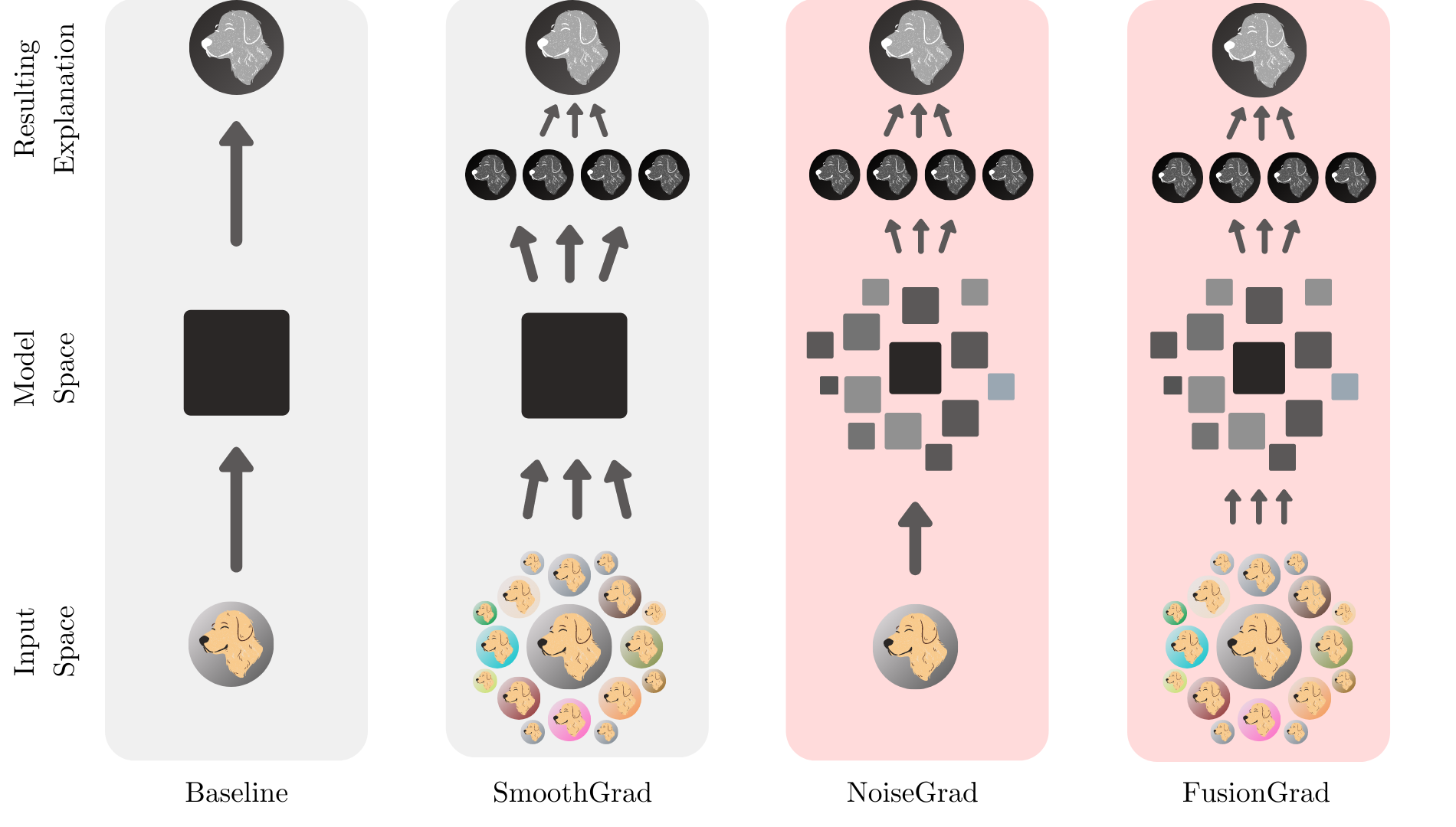
Figure 6: Illustration of our proposed methods: the functionality of the individual methods, i.e., Baseline, SmoothGrad, NoiseGrad, and FusionGrad are visualized schematically from left to right, each partitioned in input space, model space, and the resulting explanation from bottom to top. The baseline explanations are computed in a deterministic fashion – one input (dog), one model (black square), one explanation. SmoothGrad enhances the explanation by exploring the neighborhood of a datapoint, here indicated by multiple noisy versions of the input. In contrast, our proposed method, NoiseGrad, enhances the explanations by investigating the neighborhood of the trained model, indicated by multiple versions of the model. FusionGrad combines SmoothGrad and NoiseGrad by incorporating both stochasticities in the input space and model space.

Toy experiment

For the toy experiment, the dataset was generated, consisting of a total of 1024 data points, generated from an equal mixture of 4 Gaussian distributions. All 4 distributions have diagonal covariance matrix, with diagonal elements equal to 0.5 and mean values of $[8,8],[1,8],[8,1],[1,1],$ where the first 2 distributions were assigned a label 0 and last 2 distributions assigned with label 1.

Dataset was randomly split into test and training parts, test dataset consisting of 64 data points. 3-layer MLP network with ReLU activation was trained using Stochastic Gradient Descend algorithm and achieves 100 percent accuracy.

As described in the main paper, we have observed that NoiseGrad smoothens the gradients. In comparison with a SmoothGrad method, that intrinsically smoothens the gradient with convolution operation in the neighborhood of the original data point, NoiseGrad perturbs decision bound. This, in turn, results in interesting observation that could be illustrated in Figure 7 where we can observe that SG has constant gradients in the areas, where all standard (baseline) gradients have the same value, while in NG this is not happening, and all gradient in these areas slightly differ.

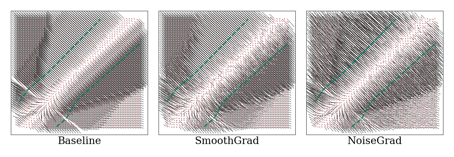
Figure 7: Comparison of smoothing effect on gradient between SmoothGrad and NoiseGrad. From left to right: standard gradient flow, SmoothGrad enhanced gradient map and NoiseGrad enhanced gradients.

Heuristic for choosing hyperparameters

For each explanation-enhancing method, we clarify the recommended heuristic i.e, the rule of thumb that was applied in the experiments to choose the right level of noise.

SmoothGrad

As suggested by the authors in (Smilkov et al. 2017), we set the standard deviation of the input noise as follows

$$\sigma_{\mathrm{SG}}=\alpha_{\mathrm{SG}}(\max(x)-\min(x)),$$ (5)

where $x$ is the input image and $\alpha_{\mathrm{SG}}$ the noise level, which is recommended by the authors to be in the interval $[0.1,0.2]$. We set $\alpha_{\mathrm{SG}}=0.2$ since with this noise level, SmoothGrad produced the explanations with the highest attribution quality in most of the cases in our experiments.

NoiseGrad

We choose $\sigma_{\mathrm{NG}}$ such that the relative accuracy drop $\textrm{AD}(\sigma_{\mathrm{NG}})$ is approximately 5 percent in all experiments. We defined the relative accuracy drop as follows:

$$\textrm{AD}(\sigma)=1-\frac{\textrm{ACC}(\sigma)-\textrm{ACC}(\infty)}{\textrm{ACC}(0)-\textrm{ACC}(\infty)},$$ (6)

where $\textrm{ACC}(0)$ and $\textrm{ACC}(\infty)$ correspond to the original accuracy and the chance level, respectively.

FusionGrad

We fix the noise level $\sigma_{\mathrm{SG}}$ for SG by Eq. (5) (setting the noise level to $\alpha_{\mathrm{SG}}=0.1$ i.e., the lower bound of the noise interval as suggested in (Smilkov et al. 2017)) and adjust the noise level $\sigma_{\mathrm{NG}}$ for NG so that the relative accuracy drop

$$\textrm{AD}_{++}(\sigma_{\mathrm{SG}},\sigma_{\mathrm{NG}})=1-\frac{\textrm{ACC}_{++}(\sigma_{\mathrm{SG}},\sigma_{\mathrm{NG}})-\textrm{ACC}(\infty)}{\textrm{ACC}_{++}(0,0)-\textrm{ACC}(\infty)}$$ (7)

is again around $\alpha_{\textrm{FG}}=0.05$. Here, $\textrm{ACC}_{++}(\sigma_{\mathrm{SG}},\sigma_{\mathrm{NG}})$ is the classification accuracy with noise levels $\sigma_{\mathrm{SG}}$ and $\sigma_{\mathrm{NG}}$ in the input image and the weight parameters, respectively.

For a better comprehension of the recommended heuristic, we report the relation between AUC value, i.e., the localization quality of the explanations, and the accuracy drop of the model (ACC) (see Eq. 6) in Figure 8. The more noise added to the weights, the higher is the accuracy drop, which is reported on the x-axis. Interestingly, we observe an increase in the AUC value, reported on the y-axis, until an accuracy drop of 5 percent. Adding more noise to the weights leads to a greater accuracy drop and causes the AUC values to decrease again.

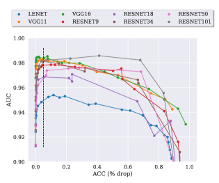
Figure 8: A visual interpretation of the proposed ”5 percent accuracy drop” noise heuristic. Each line represents a different model architecture used in the CMNIST experiment and every dot reflects the average results from 200 randomly test samples. We can observe in that general, an increase in the noise level until a drop in accuracy of $\alpha_{\mathrm{NG}}=0.05$ (black horizontal line), boosts attribution quality (AUC value).

Connection to Diagonal and KFAC Laplace approximation

As described in the main manuscript, NoiseGrad with multiplicative Gaussian noise can be seen as performing a quite crude Laplace Approximation. Yet, despite the simplicity of the proposed method, it is still sufficiently accurate to get an insight into the uncertainty of the model to enhance explanations.

We illustrate uncertainties obtained by our proposed method on a toy-task – a one-dimensional regression generated by a Gaussian Process with RBF kernel with parameters $l=1$, $\sigma=0.3$. In total we generated $400$ points, $250$ were used for training, and $150$ for testing. For training, we used a simple two-layer MLP with $10$ hidden neurons respectively and sampled $1000$ models using Hamiltonian Monte Carlo (Neal 1993) using the hamiltorch library (Cobb and Jalaian 2020). The sampled model used to perform both Kroneker-Factored (KF) and Diagonal Laplace Approximations using the curvature library (Lee et al. 2020). Finally, we visualize the uncertainty of the predictions by adding multiplicative noise to the weights using NoiseGrad, comparing it to the KFAC and Diagonal Laplace approximations. Hyperparameters for all three methods were chosen to have approximately the same loss on the test set. All results are shown in Figure 9, which demonstrates that NoiseGrad has not quite as precise, but a similar estimate of the model uncertainty as to the Bayesian approximation methods.

Empirically, from Figure 10, we can observe that explanations, which were enhanced by NoiseGrad have only slight visual differences compared to the explanations obtained by proper Laplace Approximation methods, i.e., Diagonal or KFAC. For this experiment we performed Laplace Approximation on ResNet-18, trained for multi-label classification on the PASCAL VOC 2012 dataset. Setting the NoiseGrad hyperparameter $\sigma$ to $0.1$ we searched for the hyperparameters of Diagonal and KFAC Laplace approximation such that all models had on average a similar performance on the test data.

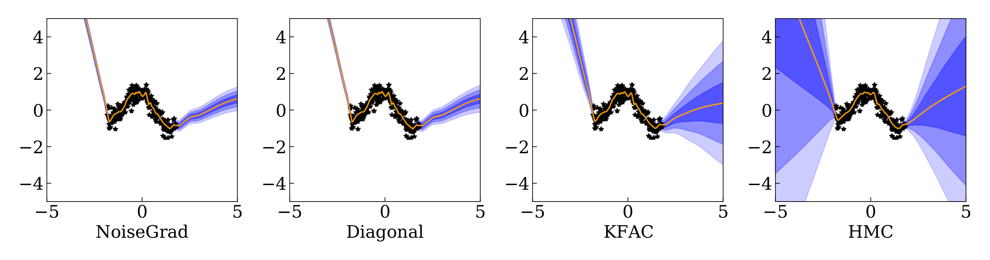
Figure 9: Toy example: comparison of NoiseGrad with Diagonal, KFAC and Hamiltonian Monte Carlo Approximation. Parameters for the NoiseGrad, Diagonal and KFAC Laplace approximations were chosen, such that they have a similar performance (MSE loss) on thee test dataset.

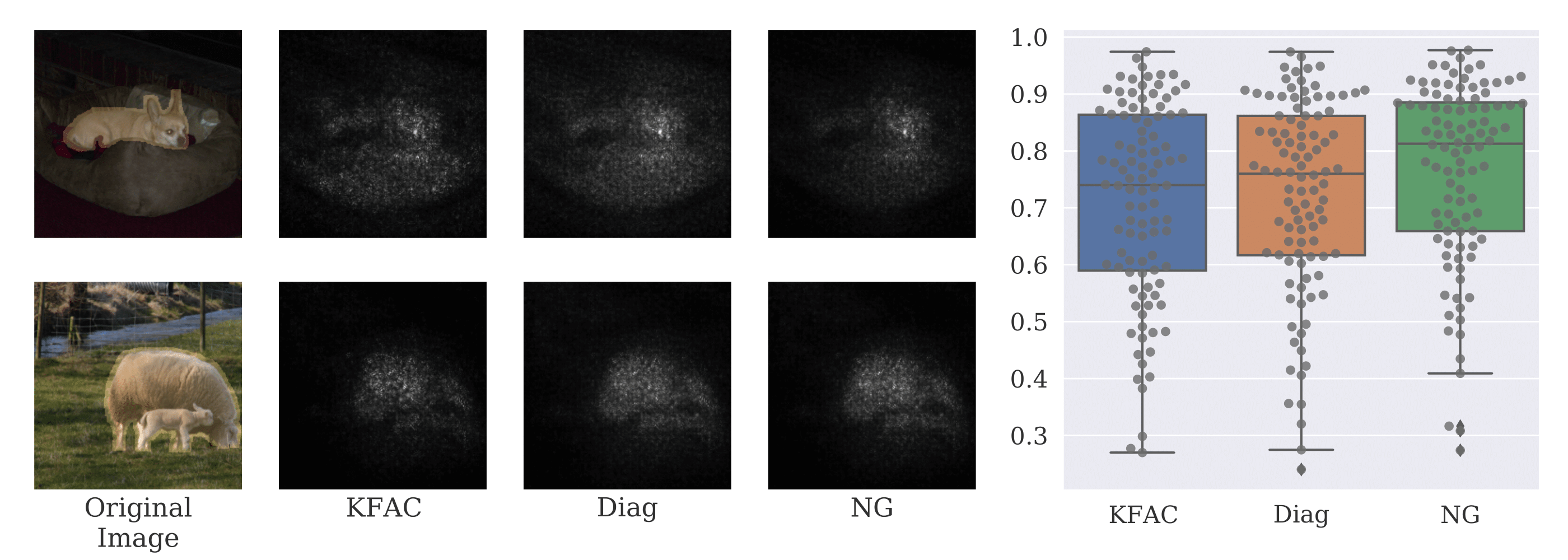
Figure 10: Comparison of the performance between our proposed method NG, KFAC and Diagonal Laplace Approximation. We can observe that the attribution quality (left: for 2 randomly chosen images) is comparable both visually and quantitatively (right: measured by $\mathrm{AUC}$) for the different approximation methods.

Experiments

In the following, we will provide additional information regarding the experimental setup as described in the main manuscript. All experiments were computed on Tesla P100-PCIE-16GB GPUs.

Evaluation methodology

In the main manuscript, we presented four properties considered useful for an explanation to fulfill. To measure the extent to which the explanations satisfied the properties, empirical interpretations are necessary. In the following paragraphs, we thus motivate and discuss choices made with respect to evaluation.

Having the object segmentation masks available for the input images, we can formulate the first property as follows

(Property 1) Localization measures the extent to which an explanation attributes its explainable evidence to the object of interest.

The higher the concentration of attribution mass on the ground-truth mask the better. For this purpose, there exist many metrics in the literature (Theiner, Müller-Budack, and Ewerth 2021; Bach et al. 2015a; Kohlbrenner et al. 2020; Zhang et al. 2018) that can be applied. Since we are interested in the attributions’ rankings and in particular, in the set of attributions covered by the ground truth (GT) mask, we apply the Relevance Rank Accuracy (Arras, Osman, and Samek 2020) as a single metric in order to assess the explanation localization. This metric computes the ratio of high-intensity relevances (or attributions) that lie within the ground truth mask. Scores range [0, 1] where higher scores are preferred. Localization is defined as follows

$$RA(E_{topK},GT)=\frac{\mid{E_{topK}}\cap GT\mid}{\mid GT\mid}$$

where $topK$ is the size of the ground truth mask and $E_{topK}=\{i_{1},i_{2},...,i_{l}\mid R_{i1}\leq R_{i2}...\leq R_{iK}\}$ (Arras, Osman, and Samek 2020). The metric counts how many of the top features lie within the ground truth mask to then divide by the size of the mask.

The second property attempts to understand whether the assigned attributions accurately reflect the behavior of the model, i.e., the faithfulness of the explanations. It is arguably one of the most well-studied evaluation metrics, hence many empirical interpretations have been proposed (Bach et al. 2015b; Montavon, Samek, and Müller 2018; Samek et al. 2016; Yeh et al. 2019; Nguyen and Martínez 2020; Alvarez Melis and Jaakkola 2018; Rieger and Hansen 2020). We define it as follows

(Property 2) Faithfulness estimates how the presence (or absence) of features influence the prediction score: removing highly important features results in model performance degradation.

To evaluate the relative fulfillment of this property, we conduct an experiment that iteratively modifies an image to measure the correlation between the sum of attributions for each modified subset of features and the difference in the prediction score (Bhatt, Weller, and Moura 2020). Given a model $f$, an explanation function $E$ and a subset $|S|$ of $d$ indices of samples $\boldsymbol{x}$ and a baseline value $\overline{{x}}$, we define faithfulness as follows

$$\mu_{\mathrm{F}}({E},{f};\boldsymbol{x})=\underset{S\in\big{(}\underset{|S|}{[d]}\big{)}}{\operatorname{corr}}\left(\sum_{i\in S}{E}({f},{x})_{i},{f}({x})-{f}\left(\boldsymbol{x}_{\left[{x}_{s}=\overline{{x}}_{s}\right]}\right)\right)$$

Due to the potential appearance of spurious correlations and creation of out-of-distribution samples, while masking original input (Hooker et al. 2018), the choice of the pixel perturbation strategy is non-trivial (Sundararajan, Taly, and Yan 2017; Sturmfels, Lundberg, and Lee 2020). For each test sample, we, therefore, average results over 100 iterations, using a subset size $|S|=32$ while setting the baseline value $\overline{{x}}$ to black. In an attempt to capture linear dependencies, the correlation metric is set to Pearson (Bhatt, Weller, and Moura 2020).

In the third property to assess attribution quality, we examine the robustness of the explanation function (Kindermans et al. 2019; Alvarez Melis and Jaakkola 2018) which, with subtle variations also is referred to as continuity (Montavon, Samek, and Müller 2018), stability (Alvarez Melis and Jaakkola 2018), coherence (Guidotti et al. 2020).

(Property 3) Robustness measures how strongly the explanations vary within a small local neighborhood of the input while the model prediction remains approximately the same.

Our empirical interpretation of robustness follows (Yeh et al. 2019) definition of max-sensitivity which is a metric that measures maximum sensitivity of an explanation when the subject is under slight perturbations, using Monte Carlo sampling-based approximation. It is defined as follows

$$\operatorname{SENS_{\operatorname{MAX}}}(E,f,{x},r)=\max_{\|{x^{\prime}}-{x}\|\leqslant r}\|E({f},{x^{\prime}})-E({f},x)\|$$

It works by constructing $n$ perturbed versions of the input $\boldsymbol{x^{\prime}}=\boldsymbol{x}+\delta$ by sampling uniformly random from a $L_{\infty}$ ball over the input, where radius=0.2 and $n$=10. By subtracting the Frobenius norms of $E(\boldsymbol{x})$ from $E(\boldsymbol{\boldsymbol{x^{\prime}}})$ we can measure the extent to which the explanations of $\boldsymbol{x}$ and $\boldsymbol{x^{\prime}}$ remained close (or distant) under these perturbations. The maximum value is computed over this set of $n$ perturbed samples. A lower value for max-sensitivity is considered better.

In the final property to assess attribution quality we were interested in studying the sparseness of the explanations since if the number of influencing features in an explanation is too large, it may be too difficult for the user to understand the explanation (Nguyen and Martínez 2020). In efforts to make human-friendly explanations, sparseness might therefore be desired. In this category of metrics, there are also complexity (Bhatt, Weller, and Moura 2020) and effective complexity (Nguyen and Martínez 2020) metrics.

(Property 4) Sparseness measures the extent to which features that are only truly predictive of the model output have significant attributions.

Following (Chalasani et al. 2020), we define sparseness as the Gini index (Hurley and Rickard 2009) of the absolute value of the attribution vector $E(\boldsymbol{x})$ where $n$ is the length of the attribution vector.

$$G(E)=\frac{\sum_{i=1}^{n}(2i-n-1)E_{i}}{n\sum_{i=1}^{n}E_{i}}$$

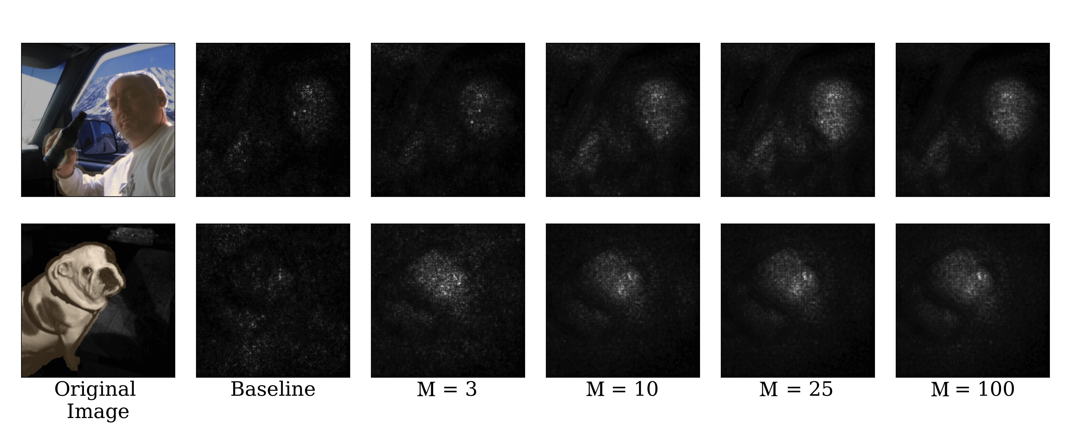
Figure 11: Saliency explanations for two randomly chosen PASCAL VOC 2012 images using NoiseGrad with different sample sizes. The quality of the explanation improves with an increasing number of samples until it no longer changes when the number of samples reaches 25.

Datasets and pre-processing

In our experiments, we use two datasets where pixel-wise placements of the explainable evidence of the attributions were made available.

CMNIST

For constructing the semi-natural dataset, we combined two well known datasets; the MNIST dataset (LeCun, Cortes, and Burges 2010), consisting of $60,000$ train- and $10,000$ test grey-scale images and the CIFAR-10 dataset, consisting of $50,000$ train- and $10,000$ test colored images. Each MNIST digit (0 to 9) was first resized from $(28,28)$ to $(16,16)$ and then rotated randomly, with a maximal rotation degree of 15. Afterward, those digits were added on top of CIFAR images of size $(32,32)$, which were uniformly sampled, such that there exists no correlation between CIFAR and MNIST classes. Hence, within this experimental setup, we could assume that the model does not rely on the background for the decision-making process. Using this constructed semi-natural dataset in the experiments, random noise of varying variance $\sigma^{2}$ was added to each CMNIST image.

As a pre-processing step, all images were normalized. For the training set, the random affine transformation was also applied to keep the image center invariant. The random rotation ranges withing $[-15,15]$ degrees, random translations, scaling and shearing in the range of $[0.95,1]$ and $[0,0.05]$ percents respectively using the fill color $0$ for standard torchvision.transforms.RandomAffine data augmentation in PyTorch (Paszke et al. 2019). We constructed three different ground-truth segmentation masks for the CMNIST dataset as follows: squared box around the digit, the digit segmentation itself, and the digit plus neighborhood of 3 pixels in each direction. In the experiments, as the evidence for a class typically also is distributed around the object itself, the squared box of $(16,16)$ pixels was selected as the single ground-truth segmentation.

PASCAL VOC 2012

We use PASCAL Visual Object Classes Challenge 2012 (VOC2012) (Everingham et al. 2010) to evaluate our method on a natural high-dimensional segmented dataset. For training and evaluation, we resize images such that the number of pixels on one axis is 224 pixels and perform center crop afterward, resulting in square images of $224\times 224$ pixels. Images are then normalized with standard ImageNet mean and standard deviation. The segmentations are also resized and cropped, accordingly. For the training we augment the data with random affine transformations that include random rotation in the range $[-30,30]$ degrees, random translations, scaling, and shearing in the range of $[0,5]$. Additionally, we perform horizontal and vertical random flips with a probability of $0.5.$

ILSVRC-15

We additionally used ImageNet Large Scale Visual Recognition Challenge (ILSVRC-15) (Russakovsky et al. 2015) to evaluate the different explanation-enhancing methods. We applied the same pre-processing as outlined for the VOC2012 dataset apart from the random affine transformations and scaling that was used for training purposes - instead, we used a ResNet-18 classifier with pre-trained weights.

Explanation methods

In this section, we provide a brief overview of the explanations methods used in the experiments conducted in both the main manuscript and the supplementary material. For each explanation method, we use absolute values of the attribution maps, following the same logic as in (Smilkov et al. 2017). This is motivated by the fact that both positive and negative attributions of explanations drive the final prediction score.

Saliency

Saliency (SA) (Mørch et al. 1995) is used as the baseline explanation method. The final relevance map quantifies the possible effects of small changes in the input on the output produced

$$E_{Saliency}\left(\boldsymbol{x},f(\cdot,W)\right)=\frac{\partial f(\boldsymbol{x},W)}{\partial\boldsymbol{x}}.$$

Integrated Gradients

Integrated Gradients (IG) (Sundararajan, Taly, and Yan 2017) is an axiomatic local explanation algorithm that also addresses the ”gradient saturation” problem. A relevance score is assigned to each feature by approximating the integral of the gradients of the models’ output with respect to a scaled version of the input (Sundararajan, Taly, and Yan 2017). The relevance attribution function for IG is defined as follows

$$E_{IG}\left(\boldsymbol{x},f(\cdot,W)\right)=\left(\boldsymbol{x}-\bar{\boldsymbol{x}}\right)\int_{0}^{1}\frac{\partial f(\boldsymbol{x}+\alpha(\boldsymbol{x}-\bar{\boldsymbol{x}}),W)}{\partial\boldsymbol{x}}d\alpha,$$

where $\bar{x}$ is a reference point, which is chosen in a way that it represents the absence of a feature in the input.

GradShap

Gradient Shap (GS) (Lundberg and Lee 2017) is a local explainability method that approximates Shapley values of the input features by computing the expected values of the gradients when adding Gaussian noise to each input. Since it computes the expectations of gradients using different reference points, it can be viewed as an approximation of IG.

Occlusion.

The occlusion method proposed in (Zeiler and Fergus 2014) is a local, model-agnostic explanation method that attributed relevances to the input by masking specific regions of the input and collecting the information about the corresponding change of the output.

LRP

Layer-wise Relevance Propagation (Bach et al. 2015b) is a model-aware explanation technique that can be applied to feed-forward neural networks and can be used for different types of inputs, such as images, videos, or text (Anders et al. 2019; Arras et al. 2017). Intuitively, the core idea of the LRP algorithm lies in the redistribution of a prediction score of a certain class towards the input features, proportionally to the contribution of each input feature. More precisely, this is done by using the weights in combination with the neural activations that were generated within the forward pass as a measure of the relevance distribution from the previous layer to the next layer until the input layer is reached. Note that this propagation procedure is subject to a conservation rule – analogous to Kirchoff’s conservation laws in electrical circuits (Montavon et al. 2019) – meaning, that in each step of back-propagation of the relevances from the output layer towards the input layer, the sum of relevances stays the same.

In the experiments we deploy the LRP gamma rule i.e., LRP-$\gamma$ which is dependent on the tuning of $\gamma$ can favor the positive attributions over negative ones. As we increase $\gamma$, negative contributions start to cancel out. The LRP gamma rule is defined as follows

$$R_{j}=\sum_{k}\frac{a_{j}\cdot\left(w_{jk}+\gamma w_{jk}^{+}\right)}{\sum_{0,j}a_{j}\cdot\left(w_{jk}+\gamma w_{jk}^{+}\right)}R_{k}$$

where $\gamma$ controls how much positive contributions are favoured, $j$ and $k$ are neurons at two consecutive layers of the network, $a_{j}$ are attributions, $w$ are weights aand $R_{k}$ are relevances.

Additional results

In the following, we present results from additional experiments.

Dependence on noise level

In the following, we investigate how the ranking of attributions in terms of the area under the curve ($\mathrm{AUC}$) (Fawcett 2006) depends on the noise levels, $\sigma_{\mathrm{SG}}$ and $\sigma_{\mathrm{NG}}$, for FusionGrad. Note that FusionGrad with $\sigma_{\mathrm{NG}}=0$ and $\sigma_{\mathrm{SG}}=0$, respectively, correspond to SmoothGrad and NoiseGrad. Figure 12 (left) shows relative AUC improvement $d\mathrm{AUC}=(\mathrm{AUC}$ / $\mathrm{AUC}_{\mathrm{Baseline}})-1)$ to the Baseline method (with zero noise levels).

From Figure 12 we can observe that the heuristics for SG, NG, and FG represents the noise levels that give the highest attribution quality in terms of ranking, which we empirically interpreted as $\mathrm{AUC}$. We also investigate the potential of our proposed methods when the noise levels are tuned by optimizing the ranking criterion. Figure 12 (right) plots the $\mathrm{AUC}$s with the optimal noise levels over 200 test samples. We observe that stochasticity in the input space and the parameter space potentially achieve the same level of attribution ranking (with smaller variance with the latter) and that their combination can further boost the performance.

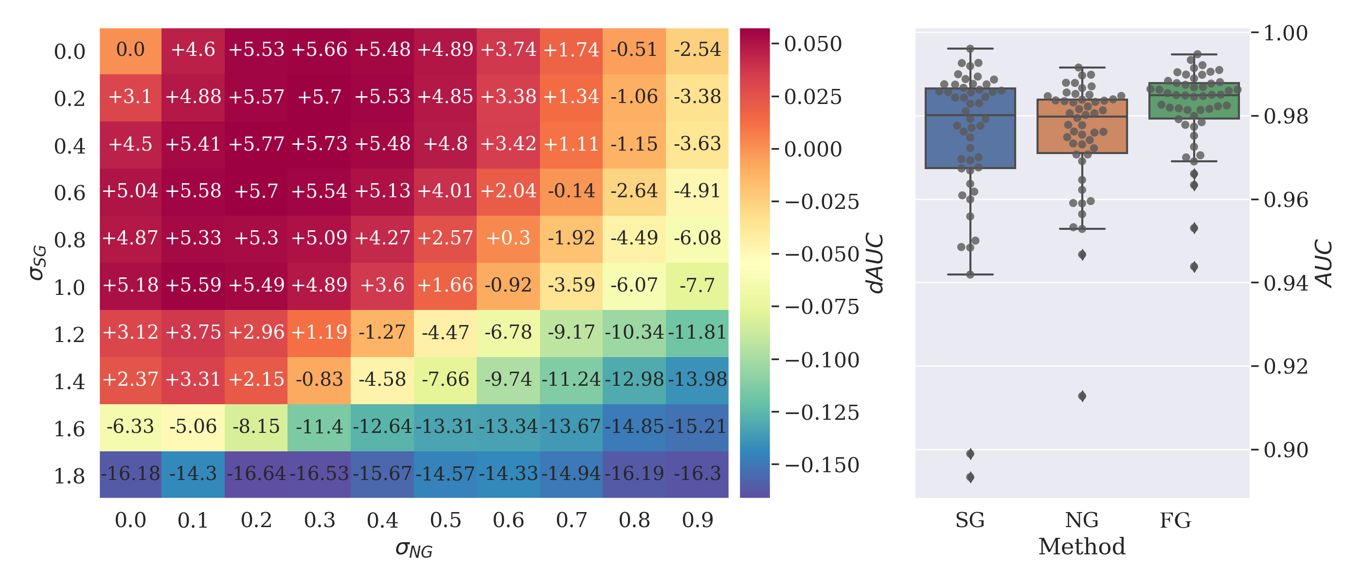
Figure 12: Left: Noise level dependence of relative AUC improvement dAUC from the Baseline method. The horizontal and the vertical axis corresponds to the noise levels $\sigma_{NG}$ and $\sigma_{SG}$. Right: the relative AUC improvement with optimal hyperparameter choice. We can observe that FG achieves better performance than SG or NG alone.

Extended table 3 - additional explanation methods

To understand how the different explanation-enhancing methods SG, NG, and FG compare to our given baseline, we scored the explanations using 4 criteria of attribution quality. The scores were computed and averaged over 256 randomly chosen test samples, using a ResNet-9 classifier. In the main manuscript, we reported on Saliency (Mørch et al. 1995) explanations. In the extended Table 3 below, results for Integrated Gradients (Sundararajan, Taly, and Yan 2017) and Gradient Shap (Lundberg and Lee 2017) are included.

As seen in Table 3, FusionGrad is significantly better than both SmoothGrad and Baseline in all evaluation criteria — that is, FusionGrad is producing more localized, faithful, robust, and sparse explanations than those baselines and competing approaches for the Integrated Gradient explanation. NoiseGrad is producing slightly higher scores than FusionGrad in robustness and faithfulness criteria, but as shown in the table, these results are not significant. Further, for Gradient Shap explanations, we can observe that in general, NoiseGrad and FusionGrad outperform the baseline- and comparison methods in this setting as well.

Table 3: Comparison of attribution quality on different explanation methods for CMNIST dataset, where the noise levels are set by the heuristic. $\uparrow$ and $\downarrow$ indicate the larger is the better and the smaller is the better, respectively. The values of the best method and the methods that are not significantly outperformed by the best method, according to the Wilcoxon signed-rank test for $p=0.05$, are bold-faced.

Explanation	Method	Localization ($\uparrow$)	Faithfulness ($\uparrow$)	Robustness ($\downarrow$)	Sparseness ($\uparrow$)
Integrated Gradients	Baseline	0.6400 $\pm$ 0.0582	0.3430 $\pm$ 0.1481	0.0556 $\pm$ 0.0163	0.7641 $\pm$ 0.0476
	SG	0.6679 $\pm$ 0.0572	0.3506 $\pm$ 0.1558	0.0585 $\pm$ 0.0211	0.7750 $\pm$ 0.0438
	NG	0.6883 $\pm$ 0.0522	0.3593 $\pm$ 0.1555	0.0170 $\pm$ 0.0048	0.8102 $\pm$ 0.0371
	FG	0.6981 $\pm$ 0.0511	0.3537 $\pm$ 0.1556	0.0179 $\pm$ 0.0049	0.8199 $\pm$ 0.0354
Gradient Shap	Baseline	0.4522 $\pm$ 0.0438	0.3623 $\pm$ 0.1625	0.1965 $\pm$ 0.0640	0.7780 $\pm$ 0.0479
	SG	0.4234 $\pm$ 0.0398	0.3629 $\pm$ 0.1535	0.1527 $\pm$ 0.0538	0.7792 $\pm$ 0.0424
	NG	0.4707 $\pm$ 0.0430	0.3650 $\pm$ 0.1589	0.1456 $\pm$ 0.0486	0.8095 $\pm$ 0.0378
	FG	0.4626 $\pm$ 0.0437	0.3603 $\pm$ 0.1536	0.1464 $\pm$ 0.0481	0.8200 $\pm$ 0.0352

Extended table 4 - additional datasets

To understand how the benefits of proposed explanation-enhancing methods NoiseGrad and FusionGrad extend to other datasets, we evaluated all the approaches using the ILSVRC-15 dataset (Russakovsky et al. 2015). The scores were computed for all four attribution quality criteria and averaged over 250 randomly chosen, normalized test samples, using a ResNet-18 classifier with pre-trained weights. As seen in the extended Table 4, explanations enhanced by FusionGrad or NoiseGrad are in most criteria outperforming both SmoothGrad and Baseline — especially when it comes to making explanations more faithful and localized. Results from three explanation methods i.e., Saliency (Mørch et al. 1995), Integrated Gradients (Sundararajan, Taly, and Yan 2017) and Gradient Shap (Lundberg and Lee 2017) are included in the table.

Table 4: Comparison of attribution quality on different explanation methods for ImageNet dataset, using noise levels $\sigma_{\mathrm{NG}}=0.2$, $\sigma_{\mathrm{SG}}=0.4758$ and $\sigma_{\mathrm{SF}}=(\sigma_{\mathrm{NG}}/2,\sigma_{\mathrm{SG}}/2)$. $\uparrow$ and $\downarrow$ indicates the larger is the better and the smaller is the better, respectively. The values of the best method and the methods that are not significantly outperformed by the best method, according to the Wilcoxon signed-rank test for $p=0.05$, are bold-faced.

Explanation	Method	Localization ($\uparrow$)	Faithfulness ($\uparrow$)	Robustness ($\downarrow$)	Sparseness ($\uparrow$)
Saliency	Baseline	0.5479 $\pm$ 0.2526	0.0209 $\pm$ 0.0660	0.0275 $\pm$ 0.0134	0.4329 $\pm$ 0.0379
	SG	0.6881 $\pm$ 0.1875	0.0330 $\pm$ 0.0683	0.0178 $\pm$ 0.0080	0.2306 $\pm$ 0.0529
	NG	0.6845 $\pm$ 0.1849	0.0340 $\pm$ 0.0682	0.0160 $\pm$ 0.0073	0.2951 $\pm$ 0.0543
	FG	0.7466 $\pm$ 0.1438	0.0405 $\pm$ 0.0710	0.0036 $\pm$ 0.0018	0.2128 $\pm$ 0.0488
Integrated Gradients	Baseline	0.5273 $\pm$ 0.2448	0.3430 $\pm$ 0.1481	0.0373 $\pm$ 0.0134	0.5718 $\pm$ 0.0379
	SG	0.5428 $\pm$ 0.1919	0.3506 $\pm$ 0.1558	0.0084 $\pm$ 0.0023	0.5378 $\pm$ 0.0333
	NG	0.5968 $\pm$ 0.1919	0.3593 $\pm$ 0.1555	0.0095 $\pm$ 0.0026	0.6013 $\pm$ 0.0486
	FG	0.5728 $\pm$ 0.2072	0.3537 $\pm$ 0.1556	0.0036 $\pm$ 0.0007	0.5548 $\pm$ 0.0415
Gradient Shap	Baseline	0.5773 $\pm$ 0.2185	0.0145 $\pm$ 0.0613	0.0384 $\pm$ 0.0152	0.6111 $\pm$ 0.0547
	SG	0.4778 $\pm$ 0.2693	0.0136 $\pm$ 0.0599	0.0019 $\pm$ 0.0006	0.5170 $\pm$ 0.0273
	NG	0.5913 $\pm$ 0.1957	0.0183 $\pm$ 0.0625	0.0077 $\pm$ 0.0021	0.5957 $\pm$ 0.0421
	FG	0.5694 $\pm$ 0.2107	0.0195 $\pm$ 0.0642	0.0040 $\pm$ 0.0007	0.5502 $\pm$ 0.0421

Sanity checks - model parameter randomization tests

In addition to the existing evaluation criteria, we also tested the relative sensitivity of the explanation-enhancing methods to the parameterization of the models using the methodology outlined in (Adebayo et al. 2018). Experimental results positively suggest that in general — explanations for the different approaches are not completely uninformative on the trained weights i.e., the rank correlation coefficient between explanations of a randomized- versus a non-randomized model $\neq 1$. The correlation coefficient is slightly higher for NG/ FG compared to SG which is due to the multiplicative noise that is added to the model weights.

Models and training results

Each model was trained similarly; using a standard cross-entropy loss (torch.nn.CrossEntropyLoss in PyTorch) – the LeNet and ResNet networks were trained using the AdamW variant (Loshchilov and Hutter 2017), with an initial learning rate of $0.001$ and the VGGs were trained using stochastic gradient descent with an initial learning rate of $0.01$ and momentum of $0.9$. The training was completed for $20$ epochs for all models. Furthermore, ReLU activations were used for all layers of the networks apart from the last layer, which employed a linear transformation. For details on model architectures we point the reader to the original source; LeNet (LeCun et al. 1998), ResNets (He et al. 2016) and VGG (Simonyan and Zisserman 2014) respectively.

In Table 5, the reader can find the model performance listed (both training- and test accuracies). For the sake of space, we refer to each ResNet as RN.

Table 5: Training results for different architectures

Acc.	LeNet	VGG11	VGG16	RN9	RN18	RN34	RN50	RN101
Train	0.7841	0.9237	0.9508	0.9723	0.9747	0.9734	0.9754	0.9760
Test	0.8653	0.9634	0.9797	0.9850	0.9864	0.9868	0.9898	0.9885

In the VOC2012 dataset, we trained a ResNet-18 for multi-label classification, changing the number of output neurons to 20 to represent the number of classes in the dataset. The network was trained with Binary Cross-Entropy loss applied on top of sigmoid layer (torch.nn.BCEWithLogitsLoss in PyTorch). ResNet-18 was initialized with ImageNet (Deng et al. 2009) pre-trained weights (available in Torchvision.models) and was trained for 100 epochs with SGD with $0.01$ learning rate and with 100 epochs with a learning rate of $0.005$. The network achieves a loss of $0.000295$ on the training dataset and $0.000376$ on the test dataset. More illustrations could be found in the Appendix.

Choosing $N$ for NG and FG

Proposed NG and FG methods can be seen as a version of a Monte-Carlo integration (Metropolis and Ulam 1949) for the following integrals:

$$I_{NG}(\boldsymbol{x})=\int_{\mathbb{R}^{S}}E\left(\boldsymbol{x},f(\cdot,\mathcal{W})\right)p(\mathcal{W})d\mathcal{W},$$

$$I_{FG}(\boldsymbol{x})=\int_{\mathbb{R}^{S}}\int_{\mathbb{R}^{d}}E\left(\boldsymbol{x}+\xi,f(\cdot,\mathcal{W}_{i})\right)p(\xi)p(\mathcal{W})d\xi d\mathcal{W}.$$

As a Monte-Carlo approximation, the standard error of the mean decreases asymptotically as $\frac{1}{\sqrt{M}}$ is independent of the dimensionality of the integral. In practice, we observe that a sample size $M\in[25,50]$ is already sufficient to generate appealing explanations as shown in Figure 11. For FG, only 10 samples for both $M$ (NG samples) and $N$ (SG samples) are enough to enhance explanations.

Related Works

While adding an element of stochasticity during back-propagation to improve generalization and robustness is nothing new in the Machine Learning community (An 1996; Gal and Ghahramani 2016; Poole, Sohl-Dickstein, and Ganguli 2014; Blundell et al. 2015) – previously, to the best of our knowledge, it was not used in the context of XAI before.

Most similar to our proposed NoiseGrad method are approaches that also inject stochasticity at inference time e.g., (Gal and Ghahramani 2016) which we also do. Our method can further be associated with ensemble modeling (Dietterich 2000), where an ensemble of predictions from several classifiers are averaged, to increase the representation of the model space or simply, reduce the risk of choosing a sub-optimal classifier. Ensemble modeling is motivated by the idea of ”wisdom of the crowd”, where a decision is based on the collective opinion of several experts (models) rather than relying on a single expert opinion (single model). In our proposed method, by averaging over a sufficiently large number of samples $N$, the idea is that the noise associated with each explanation will be approximately eliminated.

SmoothGrad (Smilkov et al. 2017) – being the main comparative method of this work – has gained a great amount of popularity since its publication. That being said, to our awareness, very few additions have been put forward when it comes to extending the idea of averaging explanations from noisy input samples. However, in the simple operation of averaging to enhance explanations, a few ideas have been proposed. The work by (Bhatt, Weller, and Moura 2020) shows that the typical error of aggregating explanation functions is less than the expected error of an explanation function alone and (Rieger and Hansen 2020) suggests a simple technique of averaging multiple explanation methods to improve robustness against manipulation.

Broader Impact

Although the use of machine learning algorithms in various application areas, such as autonomous driving or cancer cell detection, has produced astonishing achievements, the risk remains that these algorithms will make incorrect predictions. This poses a threat, especially in safety-critical areas as well as raises legal, social, and ethical questions. However, in times of advancing digitization, the deployment of artificial intelligence (AI) is often decisive for competitiveness. Therefore, methods for a thorough understanding of the often highly complex AI models are indispensable. This is where the field of explainable AI (XAI) has established itself and in recent years various XAI methods for explaining the ”black-box models” have been proposed. In general, more precise and reliable explanations of AI models would have a crucial contribution to ethical, legal, and economic requirements, the decision-making basis of the developer, and the acceptance by the end-user.

In particular, it has been shown with the explanation-enhancing SmoothGrad method, that small uncertainties, which are artificially added to the input space can lead to an improvement in the explanation. In this work, we propose a novel method, where the uncertainties are not introduced to the input space, but to the parameter space of the model. We were able to show in various experiments that this leads to a significant improvement when it comes to attribution quality of explanations, measured with different metrics, and subsequently can be beneficial in practice. In case the proposed method does not provide a localized, robust, and faithful explanation, this would have no direct consequences for the user as long as the explanation is used for decision support and is not a separate decision unit. The data we use do not contain any personal data or any offensive content.

NoiseGrad and Local Explanations

We provide further explanations of SmoothGrad, NoiseGrad, and FG for several Pascal VOC 2012 images and several different explanation methods in Figures 13-14.

Effect of number of optimization steps

One important hyper-parameter to any Activation Maximisation method is the number of optimization steps for the generation of the synthetic input. In Figures 17-18 we can observe the effect of the NoiseGrad enhancing procedure for different numbers of iterations for the optimization procedure. We can observe that enhancing effect is visible even for the low number of iterations.

Computational cost

Due to the nature of the proposed methods, the main cause for the computational complexity is the iterative perturbation of the models’ weights. Let us denote by $E$ the complexity of performing an explanation for a single input sample and a single model sample, and by $F$ the complexity of the drawing and adding/multiplying random noise to a single variable. Then, the total complexities of SG, NG, and FG are $O(N(E+DF))$, $O(N(E+PF))$, and $O(N(E+(D+P)F))$, respectively, where $N$, $D$ and $P$ are the number of (input or model) samples, the input dimension, and the parameter dimension, respectively. Therefore, the ratio between the computation time of NG (as well as FG) and that of SG is moderate for fast ($E>PF$) explanation methods (e.g., Saliency), and small for slow ($E<PF$) explanation methods (e.g., Integrated Gradient). In our experiments, for the ResNet18 we have observed that NG is roughly 7.5 times slower, and 2 times slower with Saliency and Integrated Gradient methods respectfully. In both experiments, GPU was used and $N=100$ for both methods, for CPU experiment computation time for both methods is approximately the same, as explanation complexity dominates the noise generation. For costly ($E\gg PF$) explanation methods (e.g. LIME, Occlusion) computation time can be comparable.

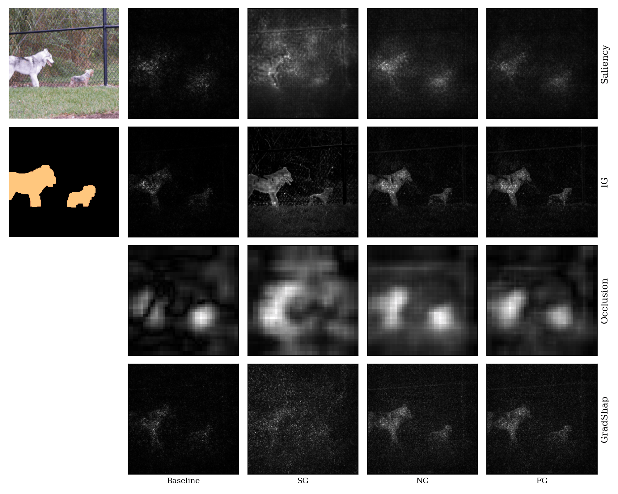
Figure 13: Comparison of different enhancing methods for class ”dog” for ImageNet dataset, using predictions from a pre-trained ResNet-18 classifier. We can observe that NG and FG methods are better in attributing relevance to the right dog, in comparison to the Baseline and SG methods.

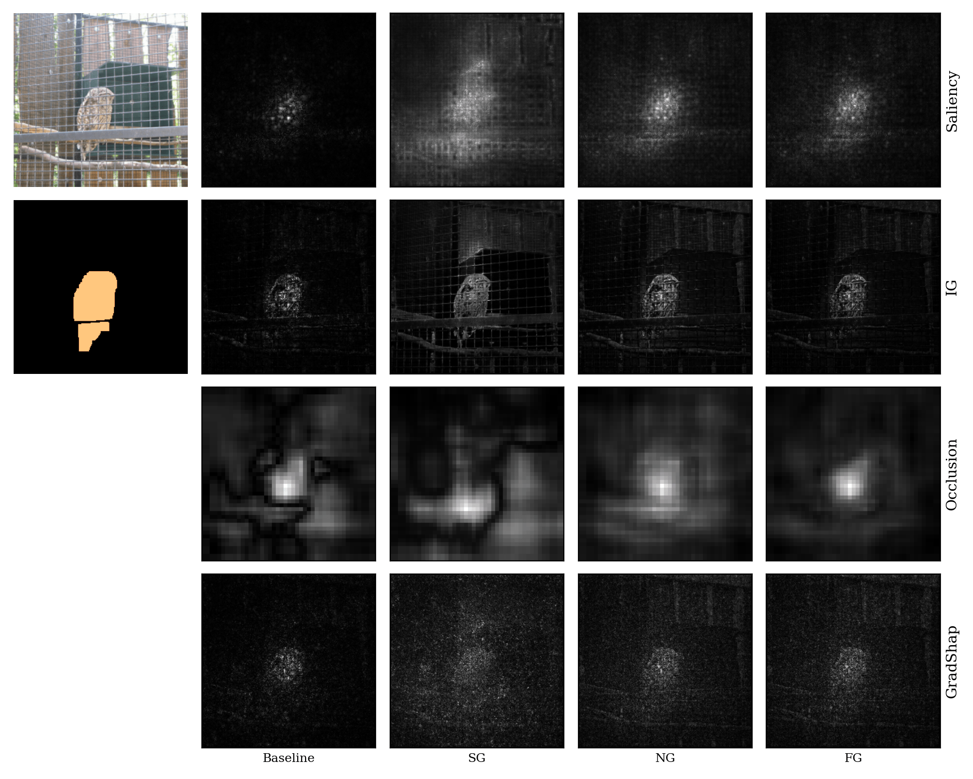
Figure 14: Comparison of different enhancing methods for class ”bird” for ImageNet dataset, using predictions from a pre-trained ResNet-18 classifier. We can observe that NG and FG place more attributional evidence at the object of interest, instead of the surroundings, like the Baseline and SG methods.

NoiseGrad and Global Explanations

We provide more examples of NoiseGrad’s enhancing capabilities towards global explanations. We used a ResNet-18 (He et al. 2016) pre-trained on Imagenet and we explained class logits with a Feature Visualisation (Olah, Mordvintsev, and Schubert 2017) method. Additional global explanations visualized in Figures 15-16.

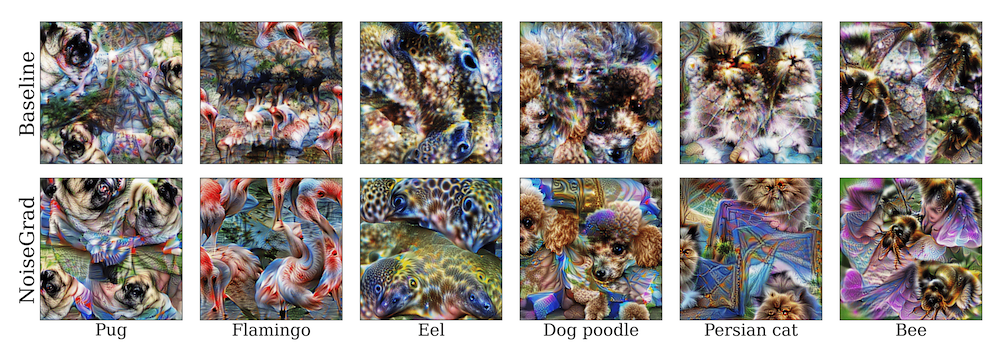
Figure 15: Comparison of standard- (top row) and NoiseGrad-enhanced (bottom row) global explanations for different classes from ImageNet dataset. By comparing the Baseline and NoiseGrad visualizations, we can observe that the abstractions generated by NoiseGrad appears to be more semantically meaningful.

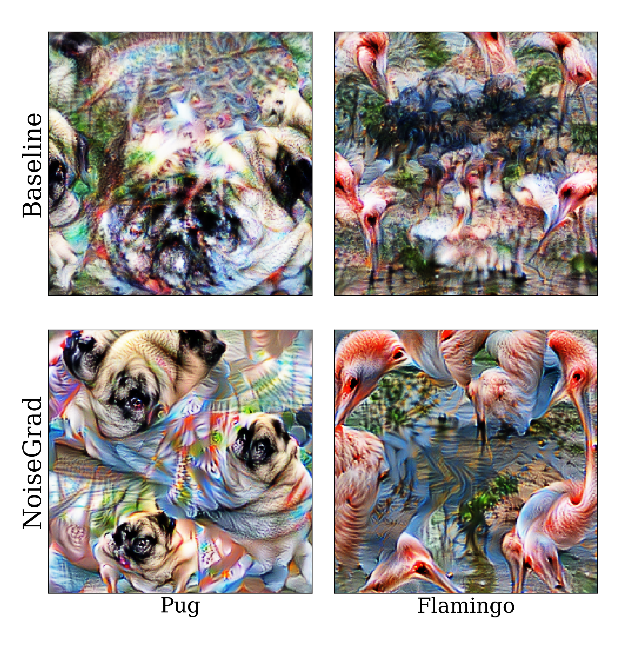
(a) Pug and Flamingo global explanations

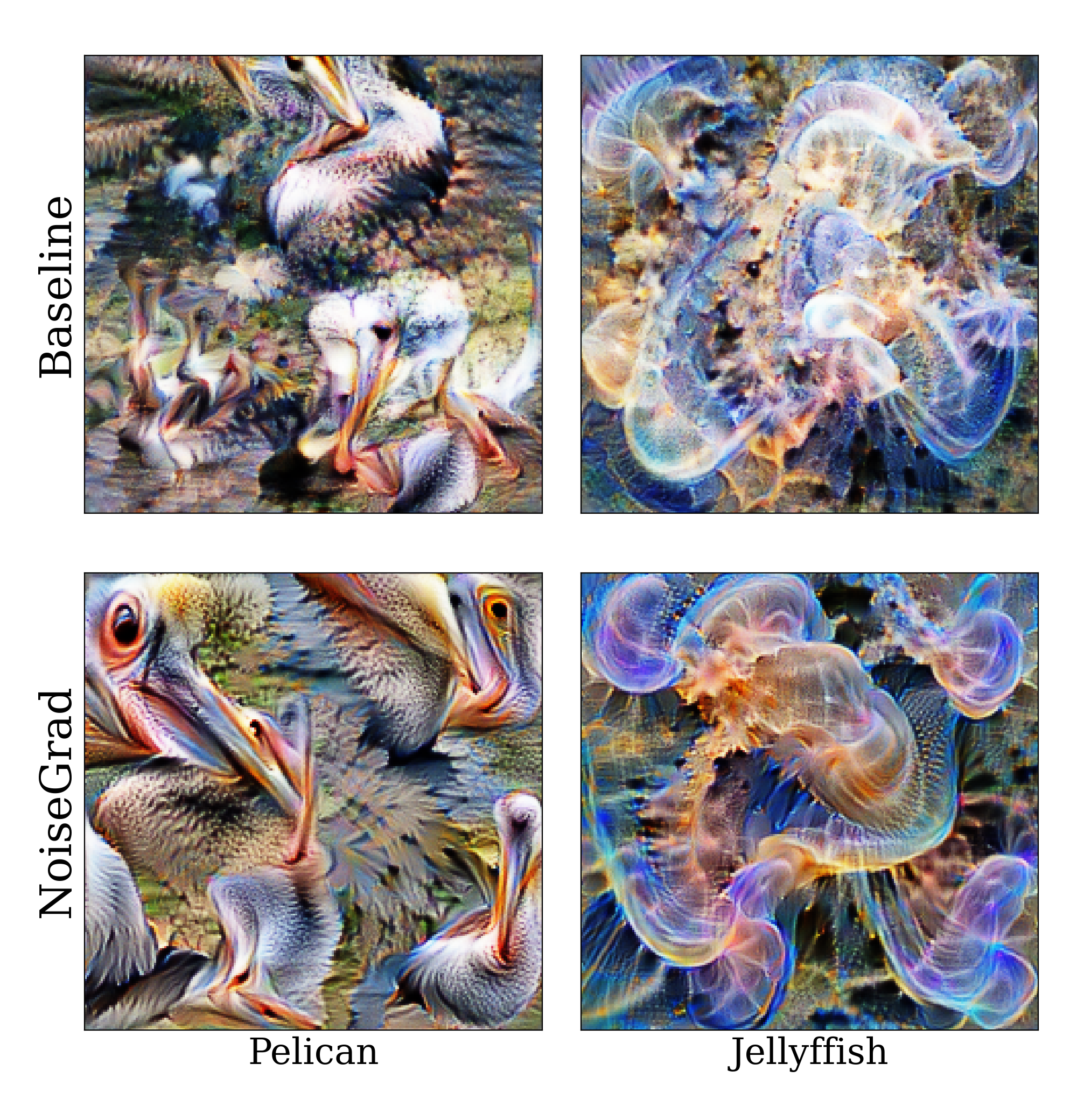
(b) Pelican and Jellyfish global explanations 2

Figure 16: Comparison of standard- (top row) and NoiseGrad-enhanced (bottom row) global explanations for different classes from ImageNet dataset. By comparing the Baseline and NoiseGrad visualizations, we can observe that the abstractions generated by NoiseGrad appears to be more semantically meaningful.

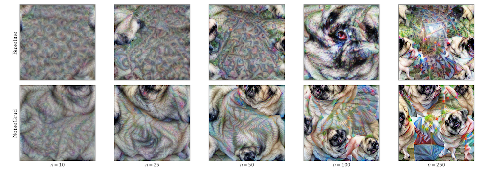
Figure 17: Comparison of standard- (top row) and NoiseGrad-enhanced (bottom row) global explanations with respect to the different number of optimizations steps for class ”Pug” from ImageNet dataset, predicted with Resnet-18 classifier.

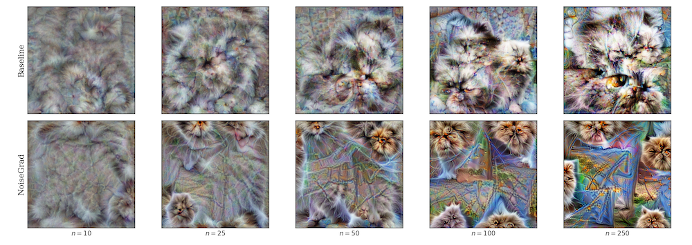
Figure 18: Comparison of standard- (top row) and NoiseGrad-enhanced (bottom row) global explanations with respect to the different number of optimizations steps for class ”Persian Cat” from ImageNet dataset, predicted with Resnet-18 classifier.

References

- Adebayo et al. (2018) Adebayo, J.; Gilmer, J.; Muelly, M.; Goodfellow, I.; Hardt, M.; and Kim, B. 2018. Sanity checks for saliency maps. In Advances in Neural Information Processing Systems, 9505–9515.
- Alvarez Melis and Jaakkola (2018) Alvarez Melis, D.; and Jaakkola, T. 2018. Towards robust interpretability with self-explaining neural networks. Advances in neural information processing systems, 31.
- An (1996) An, G. 1996. The effects of adding noise during backpropagation training on a generalization performance. Neural computation, 8(3): 643–674.
- Anders et al. (2019) Anders, C. J.; Montavon, G.; Samek, W.; and Müller, K.-R. 2019. Understanding patch-based learning of video data by explaining predictions. In Explainable AI: Interpreting, Explaining and Visualizing Deep Learning, 297–309. Springer.
- Arras et al. (2017) Arras, L.; Horn, F.; Montavon, G.; Müller, K.-R.; and Samek, W. 2017. ” What is relevant in a text document?”: An interpretable machine learning approach. PloS one, 12(8): e0181142.
- Arras, Osman, and Samek (2020) Arras, L.; Osman, A.; and Samek, W. 2020. Ground Truth Evaluation of Neural Network Explanations with CLEVR-XAI.
- Bach et al. (2015a) Bach, S.; Binder, A.; Montavon, G.; Müller, K.-R.; and Samek, W. 2015a. Analyzing Classifiers: Fisher Vectors and Deep Neural Networks.
- Bach et al. (2015b) Bach, S.; Binder, A.; on, G.; Klauschen, F.; Müller, K.-R.; and Samek, W. 2015b. On pixel-wise explanations for non-linear classifier decisions by layer-wise relevance propagation. PloS one, 10(7).
- Bhatt, Weller, and Moura (2020) Bhatt, U.; Weller, A.; and Moura, J. M. 2020. Evaluating and aggregating feature-based model explanations. arXiv preprint arXiv:2005.00631.
- Blundell et al. (2015) Blundell, C.; Cornebise, J.; Kavukcuoglu, K.; and Wierstra, D. 2015. Weight uncertainty in neural network. In International Conference on Machine Learning, 1613–1622. PMLR.
- Bykov et al. (2021) Bykov, K.; Höhne, M. M.-C.; Creosteanu, A.; Müller, K.-R.; Klauschen, F.; Nakajima, S.; and Kloft, M. 2021. Explaining Bayesian Neural Networks. arXiv preprint arXiv:2108.10346.
- Carvalho, Pereira, and Cardoso (2019) Carvalho, D. V.; Pereira, E. M.; and Cardoso, J. S. 2019. Machine learning interpretability: A survey on methods and metrics. Electronics, 8(8): 832.
- Chalasani et al. (2020) Chalasani, P.; Chen, J.; Chowdhury, A. R.; Wu, X.; and Jha, S. 2020. Concise Explanations of Neural Networks using Adversarial Training. In III, H. D.; and Singh, A., eds., Proceedings of the 37th International Conference on Machine Learning, volume 119 of Proceedings of Machine Learning Research, 1383–1391. PMLR.
- Cobb and Jalaian (2020) Cobb, A. D.; and Jalaian, B. 2020. Scaling Hamiltonian Monte Carlo Inference for Bayesian Neural Networks with Symmetric Splitting. arXiv preprint arXiv:2010.06772.
- Deng et al. (2009) Deng, J.; Dong, W.; Socher, R.; Li, L.-J.; Li, K.; and Fei-Fei, L. 2009. Imagenet: A large-scale hierarchical image database. In 2009 IEEE conference on computer vision and pattern recognition, 248–255. Ieee.
- Dietterich (2000) Dietterich, T. G. 2000. Ensemble methods in machine learning. In International workshop on multiple classifier systems, 1–15. Springer.
- Dombrowski et al. (2019) Dombrowski, A.-K.; Alber, M.; Anders, C.; Ackermann, M.; Müller, K.-R.; and Kessel, P. 2019. Explanations can be manipulated and geometry is to blame. In Advances in Neural Information Processing Systems, 13567–13578.
- Erhan et al. (2009) Erhan, D.; Bengio, Y.; Courville, A.; and Vincent, P. 2009. Visualizing higher-layer features of a deep network. University of Montreal, 1341(3): 1.
- Everingham et al. (2010) Everingham, M.; Van Gool, L.; Williams, C. K. I.; Winn, J.; and Zisserman, A. 2010. The Pascal Visual Object Classes (VOC) Challenge. International Journal of Computer Vision, 88(2): 303–338.
- Fawcett (2006) Fawcett, T. 2006. An Introduction to ROC Analysis. Pattern Recogn. Lett., 27(8): 861–874.
- Gal and Ghahramani (2016) Gal, Y.; and Ghahramani, Z. 2016. Dropout as a Bayesian Approximation: Representing Model Uncertainty in Deep Learning. In Proceedings of ICML.
- Graves (2011) Graves, A. 2011. Practical variational inference for neural networks. Advances in neural information processing systems, 24.
- Grinwald et al. (2022) Grinwald, D.; Bykov, K.; Nakajima, S.; and Höhne, M. M.-C. 2022. Visualizing the diversity of representations learned by Bayesian neural networks. arXiv preprint arXiv:2201.10859.
- Guidotti et al. (2020) Guidotti, R.; Monreale, A.; Matwin, S.; and Pedreschi, D. 2020. Black Box Explanation by Learning Image Exemplars in the Latent Feature Space. arXiv:2002.03746.
- Guidotti et al. (2018) Guidotti, R.; Monreale, A.; Ruggieri, S.; Turini, F.; Giannotti, F.; and Pedreschi, D. 2018. A survey of methods for explaining black box models. ACM computing surveys (CSUR), 51(5): 1–42.
- He et al. (2016) He, K.; Zhang, X.; Ren, S.; and Sun, J. 2016. Deep residual learning for image recognition. In Proceedings of the IEEE conference on computer vision and pattern recognition, 770–778.
- Hedström et al. (2022) Hedström, A.; Weber, L.; Bareeva, D.; Motzkus, F.; Samek, W.; Lapuschkin, S.; and Höhne, M. M. C. 2022. Quantus: An Explainable AI Toolkit for Responsible Evaluation of Neural Network Explanations.
- Hooker et al. (2018) Hooker, S.; Erhan, D.; Kindermans, P.-J.; and Kim, B. 2018. A Benchmark for Interpretability Methods in Deep Neural Networks.
- Hurley and Rickard (2009) Hurley, N.; and Rickard, S. 2009. Comparing measures of sparsity. IEEE Transactions on Information Theory, 55(10): 4723–4741.
- Kindermans et al. (2019) Kindermans, P.-J.; Hooker, S.; Adebayo, J.; Alber, M.; Schütt, K. T.; Dähne, S.; Erhan, D.; and Kim, B. 2019. The (un) reliability of saliency methods. In Explainable AI: Interpreting, Explaining and Visualizing Deep Learning, 267–280. Springer.
- Kingma, Salimans, and Welling (2015) Kingma, D. P.; Salimans, T.; and Welling, M. 2015. Variational Dropout and the Local Reparameterization Trick. In Advances in NIPS.
- Kohlbrenner et al. (2020) Kohlbrenner, M.; Bauer, A.; Nakajima, S.; Binder, A.; Samek, W.; and Lapuschkin, S. 2020. Towards Best Practice in Explaining Neural Network Decisions with LRP. arXiv:1910.09840.
- Krizhevsky, Hinton et al. (2009) Krizhevsky, A.; Hinton, G.; et al. 2009. Learning multiple layers of features from tiny images.
- LeCun et al. (1998) LeCun, Y.; Bottou, L.; Bengio, Y.; and Haffner, P. 1998. Gradient-based learning applied to document recognition. Proceedings of the IEEE, 86(11): 2278–2324.
- LeCun, Cortes, and Burges (2010) LeCun, Y.; Cortes, C.; and Burges, C. 2010. MNIST handwritten digit database. ATT Labs [Online]. Available: http://yann.lecun.com/exdb/mnist, 2.
- Lee et al. (2020) Lee, J.; Humt, M.; Feng, J.; and Triebel, R. 2020. Estimating Model Uncertainty of Neural Networks in Sparse Information Form. In International Conference on Machine Learning (ICML). Proceedings of Machine Learning Research.
- Loshchilov and Hutter (2017) Loshchilov, I.; and Hutter, F. 2017. Decoupled weight decay regularization. arXiv preprint arXiv:1711.05101.
- Lundberg and Lee (2017) Lundberg, S. M.; and Lee, S.-I. 2017. A unified approach to interpreting model predictions. In Advances in neural information processing systems, 4765–4774.
- Metropolis and Ulam (1949) Metropolis, N.; and Ulam, S. 1949. The monte carlo method. Journal of the American statistical association, 44(247): 335–341.
- Molchanov, Ashukha, and Vetrov (2017) Molchanov, D.; Ashukha, A.; and Vetrov, D. 2017. Variational Dropout Sparsifies Deep Neural Networks. In Proceedings of ICML.
- Montavon et al. (2019) Montavon, G.; Binder, A.; Lapuschkin, S.; Samek, W.; and Müller, K.-R. 2019. Layer-wise relevance propagation: an overview. In Explainable AI: Interpreting, Explaining and Visualizing Deep Learning, 193–209. Springer.
- Montavon, Samek, and Müller (2018) Montavon, G.; Samek, W.; and Müller, K.-R. 2018. Methods for interpreting and understanding deep neural networks. Digital Signal Processing, 73: 1–15.
- Mørch et al. (1995) Mørch, N. J. S.; Kjems, U.; Hansen, L. K.; Svarer, C.; Law, I.; Lautrup, B.; Strother, S. C.; and Rehm, K. 1995. Visualization of neural networks using saliency maps. In Proceedings of International Conference on Neural Networks (ICNN’95), Perth, WA, Australia, November 27 - December 1, 1995, 2085–2090. IEEE.
- Mordvintsev, Olah, and Tyka (2015) Mordvintsev, A.; Olah, C.; and Tyka, M. 2015. Inceptionism: Going Deeper into Neural Networks. https://research.googleblog.com/2015/06/inceptionism-going-deeper-into-neural.html. Accessed: 2022-04-25.
- Neal (1993) Neal, R. M. 1993. Bayesian learning via stochastic dynamics. In Advances in neural information processing systems, 475–482.
- Nguyen et al. (2016) Nguyen, A.; Dosovitskiy, A.; Yosinski, J.; Brox, T.; and Clune, J. 2016. Synthesizing the preferred inputs for neurons in neural networks via deep generator networks. In Advances in neural information processing systems, 3387–3395.
- Nguyen and Martínez (2020) Nguyen, A.; and Martínez, M. R. 2020. On quantitative aspects of model interpretability. arXiv preprint arXiv:2007.07584.
- Olah, Mordvintsev, and Schubert (2017) Olah, C.; Mordvintsev, A.; and Schubert, L. 2017. Feature visualization. Distill, 2(11): e7.
- Osawa et al. (2019) Osawa, K.; Swaroop, S.; Jain, A.; Eschenhagen, R.; Turner, R. E.; Yokota, R.; and Khan, M. E. 2019. Practical Deep Learning with Bayesian Principles. In Advances in NeurIPS.
- Paszke et al. (2019) Paszke, A.; Gross, S.; Massa, F.; Lerer, A.; Bradbury, J.; Chanan, G.; Killeen, T.; Lin, Z.; Gimelshein, N.; Antiga, L.; Desmaison, A.; Kopf, A.; Yang, E.; DeVito, Z.; Raison, M.; Tejani, A.; Chilamkurthy, S.; Steiner, B.; Fang, L.; Bai, J.; and Chintala, S. 2019. PyTorch: An Imperative Style, High-Performance Deep Learning Library. In Wallach, H.; Larochelle, H.; Beygelzimer, A.; d'Alché-Buc, F.; Fox, E.; and Garnett, R., eds., Advances in Neural Information Processing Systems 32, 8024–8035. Curran Associates, Inc.
- Poole, Sohl-Dickstein, and Ganguli (2014) Poole, B.; Sohl-Dickstein, J.; and Ganguli, S. 2014. Analyzing noise in autoencoders and deep networks. arXiv preprint arXiv:1406.1831.
- Rieger and Hansen (2020) Rieger, L.; and Hansen, L. K. 2020. A simple defense against adversarial attacks on heatmap explanations. arXiv preprint arXiv:2007.06381.
- Ritter, Botev, and Barber (2018) Ritter, H.; Botev, A.; and Barber, D. 2018. A scalable laplace approximation for neural networks. In 6th International Conference on Learning Representations, ICLR 2018-Conference Track Proceedings, volume 6. International Conference on Representation Learning.
- Romijnders (2017) Romijnders, R. 2017. Simple Semantic Segmentation. https://github.com/RobRomijnders/segm. Accessed: 2022-04-25.
- Russakovsky et al. (2015) Russakovsky, O.; Deng, J.; Su, H.; Krause, J.; Satheesh, S.; Ma, S.; Huang, Z.; Karpathy, A.; Khosla, A.; Bernstein, M.; Berg, A. C.; and Fei-Fei, L. 2015. ImageNet Large Scale Visual Recognition Challenge. International Journal of Computer Vision (IJCV), 115(3): 211–252.
- Samek et al. (2016) Samek, W.; Binder, A.; on, G.; Lapuschkin, S.; and Müller, K.-R. 2016. Evaluating the visualization of what a deep neural network has learned. IEEE transactions on neural networks and learning systems, 28(11): 2660–2673.
- Samek et al. (2021) Samek, W.; Montavon, G.; Lapuschkin, S.; Anders, C. J.; and Müller, K.-R. 2021. Explaining deep neural networks and beyond: A review of methods and applications. Proceedings of the IEEE, 109(3): 247–278.
- Selvaraju et al. (2019) Selvaraju, R. R.; Cogswell, M.; Das, A.; Vedantam, R.; Parikh, D.; and Batra, D. 2019. Grad-CAM: Visual Explanations from Deep Networks via Gradient-Based Localization. International Journal of Computer Vision, 128(2): 336–359.
- Simonyan and Zisserman (2014) Simonyan, K.; and Zisserman, A. 2014. Very deep convolutional networks for large-scale image recognition. arXiv preprint arXiv:1409.1556.
- Smilkov et al. (2017) Smilkov, D.; Thorat, N.; Kim, B.; Viégas, F.; and Wattenberg, M. 2017. Smoothgrad: removing noise by adding noise. arXiv preprint arXiv:1706.03825.
- Sturmfels, Lundberg, and Lee (2020) Sturmfels, P.; Lundberg, S.; and Lee, S.-I. 2020. Visualizing the impact of feature attribution baselines. Distill, 5(1): e22.
- Sundararajan, Taly, and Yan (2017) Sundararajan, M.; Taly, A.; and Yan, Q. 2017. Axiomatic attribution for deep networks. In International Conference on Machine Learning, 3319–3328. PMLR.
- Theiner, Müller-Budack, and Ewerth (2021) Theiner, J.; Müller-Budack, E.; and Ewerth, R. 2021. Interpretable Semantic Photo Geolocalization. arXiv:2104.14995.
- Vidovic et al. (2016) Vidovic, M. M.-C.; Görnitz, N.; Müller, K.-R.; and Kloft, M. 2016. Feature importance measure for non-linear learning algorithms. arXiv preprint arXiv:1611.07567.
- Wenzel et al. (2020) Wenzel, F.; Roth, K.; Veeling, B. S.; Swiatkowski, J.; Tran, L.; Mandt, S.; Snoek, J.; Salimans, T.; Jenatton, R.; and Nowozin, S. 2020. How Good is the Bayes Posterior in Deep Neural Networks Really? arXiv:2002.02405.
- Yang and Kim (2019) Yang, M.; and Kim, B. 2019. Benchmarking Attribution Methods with Relative Feature Importance. CoRR, abs/1907.09701.
- Yeh et al. (2019) Yeh, C.-K.; Hsieh, C.-Y.; Suggala, A. S.; Inouye, D. I.; and Ravikumar, P. 2019. On the (in) fidelity and sensitivity for explanations. arXiv preprint arXiv:1901.09392.
- Zeiler and Fergus (2014) Zeiler, M. D.; and Fergus, R. 2014. Visualizing and understanding convolutional networks. In European conference on computer vision, 818–833. Springer.
- Zhang et al. (2018) Zhang, J.; Bargal, S. A.; Lin, Z.; Brandt, J.; Shen, X.; and Sclaroff, S. 2018. Top-down neural attention by excitation backprop. International Journal of Computer Vision, 126(10): 1084–1102.