Backreaction from inhomogeneous matter fields during large-scale structure formation

Abstract

We study how inhomogeneities of the cosmological fluid fields backreact on the homogeneous part of energy density and how they modify the Friedmann equations. In general, backreaction requires to go beyond the pressureless ideal fluid approximation, and this can lead to a reduced growth of cosmological large scale structure. Since observational evidence favours evolution close to the standard growing mode in the linear regime, we focus on two-component fluids in which the non-ideal fluid is gravitationally coupled to cold dark matter and in which a standard growing mode persists. This is realized, e.g. for a baryonic fluid coupled to cold dark matter. We calculate the backreaction for this case and for a wide range of other two-fluid models. Here the effect is either suppressed because the non-ideal matter properties are numerically too small, or because they lead to a too stringent UV cut-off of the integral over the power spectrum that determines backreaction. We discuss then matter field backreaction from a broader perspective and generalize the formalism such that also far-from-equilibrium scenarios relevant to late cosmological times and non-linear scales can be addressed in the future.

I Introduction

The evolution equations used in cosmology are usually obtained under the assumption of a spatially homogeneous and isotropic distribution of matter. Although these symmetries remain preserved at all times in a statistical sense, the deviations from homogeneity and isotropy become locally sizeable during cosmological large-scale structure formation at late times. Here we ask whether this can have any influence on the cosmological evolution equations.

Because Einsteins gravitational field equations are non-linear, this question amounts to asking whether the Einstein equations for spatially averaged fields are affected by so-called backreaction effects, i.e., averages of second and higher orders in spatial inhomogeneities. Arguments that such backreaction effects are always irrelevant for cosmology have been made Green:2016cwo and have been contested Buchert:2015iva ; Buchert:2011sx , the discussion focussing mainly on inhomogeneities of the metric. The smallness of the gravitational coupling constant $G_{\text{N}}$ makes it plausible that terms non-linear in inhomogeneities of the metric remain negligible for cosmological evolution Wetterich:2001kr ; Green:2010qy .

However, the Einstein equations contain also the energy-momentum tensor of the matter distribution which develops large inhomogeneities. Starting from an approximation of matter fields as a non-ideal fluid, it was demonstrated in Ref. Floerchinger:2014jsa how such inhomogeneities give rise to backreaction effects in late-time cosmology where non-linear terms in metric inhomogeneities and their temporal variations are negligible compared to those of inhomogeneities in the matter fields.

The purpose of the present manuscript is two-fold. First, we provide within the formalism of Ref. Floerchinger:2014jsa the first explicit calculations of backreaction effects in dynamical model scenarios. Second, we generalize the formalism of Ref. Floerchinger:2014jsa to systems in which a Navier-Stokes fluid description cannot be taken for granted.

II Backreaction formalism

As derived in Ref. Floerchinger:2014jsa , backreaction effects in a Friedmann-Robertson-Walker (FRW) universe can be encoded in a time or scale-factor dependent source term $D(a)$ for the evolution of the spatially averaged energy density $\bar{\varepsilon}$,

$$\tfrac{1}{a}\dot{\bar{\varepsilon}}+3H\,(\bar{\varepsilon}+\bar{p}_{\text{eff}})=D(a)\,.$$ (1)

Here, the Hubble constant $H=\dot{a}/a^{2}$ is expressed in terms of the scale factor $a(\tau)$ of the FRW metric $ds^{2}=a^{2}\left[-d\tau^{2}+\delta_{ij}dx^{i}\,dx^{j}\right]$ and the dot denotes a derivative with respect to conformal time $\tau$. The effective pressure $\bar{p}_{\text{eff}}=\bar{p}+\bar{\pi}_{\text{bulk}}$ contains thermal pressure and a possible bulk viscous modification. Eq. (1) holds irrespective of whether a fluid description of the matter distribution with inhomogeneities is applicable (see section IV for details), but the explicit form of $D$ depends on it.

The spatial average of the trace of the Einstein field equations can be shown to be free of backreaction effects,

$$\frac{\ddot{a}}{a^{3}}=\frac{1}{a}\dot{H}+2H^{2}=\frac{4\pi G_{\text{N}}}{3}\left(\bar{\varepsilon}-3\bar{p}_{\text{eff}}\right)\,.$$ (2)

Combined with the energy conservation (1), this closes the evolution equations for background fields. The two equations combine to

$$aD=\frac{1}{a^{4}}\frac{d}{d\tau}\left[a^{4}\bar{\varepsilon}\right]-\frac{3}{8\pi G_{N}}\frac{1}{a^{4}}\frac{d}{d\tau}\left[{\dot{a}}^{2}\right]\,.$$ (3)

Integrating over $\tau$, one finds the modified Friedmann equation

$$H^{2}(\tau) = \left(\frac{{\dot{a}}(\tau)}{a^{2}(\tau)}\right)^{2}$$

$$= \frac{8\pi G_{N}}{3}\left(\bar{\varepsilon}(\tau)-\frac{1}{a^{4}(\tau)}\int_{\tau_{i}}^{\tau}d\tau^{\prime}a^{5}(\tau^{\prime})D(\tau^{\prime})\right)\,,$$

where we have assumed that the backreaction $D(\tau^{\prime})$ vanishes for sufficiently early times $\tau^{\prime}<\tau_{i}$. We emphasize that (II) holds irrespective of whether a fluid approximation applies.

Further consequences of (II) are explored in Appendix A. In particular, we show that if backreaction arises in a purely radiative sector, the $D$-dependent contribution to $\bar{\varepsilon}(\tau)$ in eq. (II) cancels exactly the second term on the right hand side, so that $H(\tau)$ is in this sence $D$-independent. For other equations of state, however, the $D$-dependence does not cancel in eq. (II), i.e., the Friedmann equation is modified.

III Linearized Inhomogeneitites and backreaction in cosmological fluids

In this section, we first consider cosmological matter fields in dynamical scenarios for which fluid dynamics applies and where inhomogeneities can be followed by linearized fluid equations. The backreaction formalism of section II can then be elaborated on in detail.

III.1 The backreaction term for a fluid

For the case that matter fields can be described as non-ideal fluids with finite pressure and/or non-vanishing shear- and bulk viscosities $\bar{\zeta}$ and $\bar{\eta}$, the backreaction term $D(a)$ can be written explicitly as Floerchinger:2014jsa

$$D = -\frac{1}{a}\int d^{3}qP_{\theta p}(\vec{q})$$ (5)

$$+\frac{1}{a^{2}}\left(\bar{\zeta}+\frac{4}{3}\bar{\eta}\right)\int d^{3}qP_{\theta\theta}(\vec{q})$$

$$+\frac{1}{a^{2}}\bar{\eta}\int d^{3}q\left(P_{w}\right)_{jj}(\vec{q})\,.$$

Here, $\left\langle\tilde{\theta}\left(\vec{q}_{1}\right)\tilde{\theta}\left(\vec{q}_{2}\right)\right\rangle=\delta^{(3)}\left(\vec{q}_{1}+\vec{q}_{2}\right)P_{\theta\theta}\left(\vec{q}_{1}\right)$ defines the power spectrum $P_{\theta\theta}$ in terms of a spatial average $\langle\dots\rangle$ of the expansion scalar $\theta(x)=\int d^{3}q\,{\tilde{\theta}}(q)e^{iqx}$. The spectra for vorticity $w$ and pressure $p$ are defined analogously.

To understand how to arrive at (5), one may consider the case of a fluid with pressure but with vanishing viscosities. The fluid dynamic equation for the energy density takes then the form

$$\dot{\varepsilon}+\vec{v}\cdot\vec{\nabla}\varepsilon+(\varepsilon+p)\left(3\frac{\dot{a}}{a}+\vec{\nabla}\cdot\vec{v}\right)=0\,.$$ (6)

Here, the flow field $u^{\mu}=(\gamma,\gamma\vec{v})$ with $\gamma=1/a\sqrt{1-v^{2}}$ allows for small inhomogeneities $|\vec{v}|\ll 1$ on top of the Hubble flow. The combination $\vec{v}\cdot\vec{\nabla}\varepsilon+\varepsilon\,\vec{\nabla}\cdot\vec{v}$ is a total derivative with vanishing spatial average and therefore,

$$\tfrac{1}{a}\dot{\bar{\varepsilon}}+3H\,(\bar{\varepsilon}+\bar{p})=\tfrac{1}{a}\langle\vec{v}\cdot\vec{\nabla}p\rangle=-\tfrac{1}{a}\langle\delta p\,\vec{\nabla}\cdot\vec{v}\rangle\,.$$ (7)

The spatial average $\langle\delta p\,\vec{\nabla}\cdot\vec{v}\rangle$ over second order perturbations can then be expressed in terms of an integral over the power spectrum $P_{\theta p}(\vec{q})$. This is the first line of (5). One obtains the last two lines in (5) by including the shear and bulk viscous contributions in the Navier-Stokes approximation in eq. (6) and following the same derivation.

III.2 Non-ideal fluids with standard growing modes

The main aim of the present section is to calculate $D$ explicitly for model scenarios of large-scale structure formation in which cosmological matter is treated in the fluid approximation. To this end, we expose first some qualitative considerations which inform our choice of model scenarios:

The growth of large scale structure after photon decoupling is thought to follow a growing mode approximately $\propto a$. This growing mode is realized, e.g., when cold dark matter (CDM) is described as an ideal fluid. However, the term $D$ in (5) vanishes for a pressure-less and non-viscous ideal fluid. On the other hand, one-component fluids with pressure and/or viscosity are known to show a modified growth of cosmological large scale structure Li:2009mf ; Velten:2011bg ; Gagnon:2011id ; viscous ; Barbosa:2017ojt . For instance, for a one-component fluid with pressure, the Jeans criterion implies that over-densities oscillate rather than grow if their mass is below the Jeans mass. This shows that it is not easy to generate any backreaction without modifying the late-time power-law growth of cosmological large scale structure.

In building cosmological models with backreaction, one bold approach could be to start without taking into account any constraint from the approximately linear growth of large scale structure; one may hope that at least some of the models constructed this way evade existing constraints or indicate modifications that will be supported by future observations. Alternatively, a very conservative approach would be to restrict the study to cosmological models which show a linear growing mode at all scales and which are therefore designed to pass observational constraints on large scale structure. In the following, we adopt this conservative approach.

Two-component fluids in which a fluid with pressure and/or viscosity is coupled gravitationally to a pressure-less fluid show a standard linear growing mode in linear perturbation theory. One well-known case is a fluid with pressure coupled to a pressure-less fluid. This is realized, e.g., in the $\Lambda$CDM model where baryonic matter retains after recombination a small ionization and thus a small pressure. It is then the gravitational coupling to pressure-less cold dark matter that ensures the growth $\propto a$ of the density contrast of baryonic matter on all scales, while the baryonic pressure does some work during the same epoch. We calculate the very small backreaction effect for this $\Lambda$CDM scenario in section III.4 before investigating other two-component models that allow for somewhat larger backreaction effects.

III.3 Gravitationally coupled two-component fluids

For a one-component fluid with pressure and finite viscosity, the equations of motion for the expansion scalar $\theta_{\mathbf{k}}$ and the energy density contrast $\delta_{\mathbf{k}}\equiv\delta\varepsilon_{\mathbf{k}}/\bar{\varepsilon}$ read at linear order and for subhorizon fluctuations

$$\dot{\delta}_{\mathbf{k}} = -(1+w)\theta_{\mathbf{k}}-3{\cal H}(c^{2}_{s}-w)\delta_{\mathbf{k}}\,,$$ (8)

$$\dot{\theta}_{\mathbf{k}} = -(1-3c^{2}_{ad}){\cal H}\theta_{\mathbf{k}}+k^{2}\Psi_{\mathbf{k}}$$ (9)

$$+\frac{c^{2}_{s}}{1+w}k^{2}\delta_{\mathbf{k}}-\frac{4}{3}k^{2}\frac{\eta}{(1+w)\bar{\varepsilon}a}\theta_{\mathbf{k}}\,,$$

$$k^{2}\Phi_{\mathbf{k}} = -\frac{3}{2}{\cal H}^{2}\delta_{\mathbf{k}}\,,$$ (10)

$$k^{2}\Psi_{\mathbf{k}} = -\frac{3}{2}{\cal H}^{2}\left(\delta_{\mathbf{k}}+4\frac{\eta}{(1+w)\bar{\varepsilon}a}\theta_{\mathbf{k}}\right)\,.$$ (11)

Here, the subscript $\mathbf{k}$ denotes Fourier modes of wavelength $2\pi/k$ and eqs. (10) and (11) are the Poisson equations for the two Newtonian potentials $\Phi_{\mathbf{k}}$ and $\Psi_{\mathbf{k}}$. We have parametrized the equation of state in terms of

$$w = \frac{\bar{p}}{\bar{\varepsilon}}\,,~{}~{}c^{2}_{s}=\frac{dp}{d\varepsilon}\,,~{}~{}c^{2}_{ad}=\frac{\dot{\bar{p}}}{\dot{\bar{\varepsilon}}}=w-\frac{\dot{w}}{3(1+w)}{\cal H}\,,\qquad$$ (12)

where $H={\cal H}/a$ and where $c_{s}$ denotes the velocity of sound. We assume in the following that $w$, $c_{s}$, $c_{ad}$, $\eta{\cal H}/(\bar{\varepsilon}a)$ are much smaller than 1, so that we can set them equal to 0, apart from terms in which they are multiplied by $k^{2}$. In this approximation, the shear viscous difference between the two Newtonian potentials is neglected, $\Phi_{\mathbf{k}}=\Psi_{\mathbf{k}}$.

We now consider two sectors: one with pressure and/or shear viscosity that gives rise to a backreaction $D$ (we denote it therefore by a subscript $D$), and one which is standard pressure-less and non-viscous cold dark matter (subscript $C$). The spatially averaged energy densities of both sectors evolve independent of each other, but it is the sum of their gravitational attractions that enters the trace of Einstein’s field equations and that determines the expansion history. This is seen in the background equations

$$\frac{1}{a}\dot{\bar{\varepsilon}}_{D}+3H\,\bar{\varepsilon}_{D}=D\,,$$ (13)

$$\frac{1}{a}\dot{\bar{\varepsilon}}_{C}+3H\,\bar{\varepsilon}_{C}=0\,,$$ (14)

$$\frac{\ddot{a}}{a^{3}}=\frac{1}{a}\dot{H}+2H^{2}=\frac{4\pi G_{\text{N}}}{3}(\bar{\varepsilon}_{D}+\bar{\varepsilon}_{C})\,.$$ (15)

We denote matter inhomogeneities in the two sectors by ${\delta}_{\mathbf{k}}$, ${\theta}_{\mathbf{k}}$ and ${d}_{\mathbf{k}}$, ${\vartheta}_{\mathbf{k}}$, respectively. To linear order, these inhomogeneities are coupled gravitationally via the Poisson equation,

$$\dot{\delta}_{\mathbf{k}} = -\theta_{\mathbf{k}}\,,$$ (16)

$$\dot{\theta}_{\mathbf{k}} = -{\cal H}\theta_{\mathbf{k}}+k^{2}\Psi_{\mathbf{k}}+c^{2}_{s}k^{2}\delta_{\mathbf{k}}-\frac{4}{3}k^{2}\frac{\eta}{\bar{\varepsilon}_{D}a}\theta_{\mathbf{k}}\,,$$ (17)

$$\dot{d}_{\mathbf{k}} = -\vartheta_{\mathbf{k}}\,,$$ (18)

$$\dot{\vartheta}_{\mathbf{k}} = -{\cal H}\vartheta_{\mathbf{k}}+k^{2}\Psi_{\mathbf{k}}\,,$$ (19)

$$k^{2}\Psi_{\mathbf{k}} = -\frac{3}{2}{\cal H}^{2}\left(\Omega_{C}d_{\mathbf{k}}+\Omega_{D}\delta_{\mathbf{k}}\right)\,,$$ (20)

where $\Omega_{D}\equiv\varepsilon_{D}/(\varepsilon_{D}+\varepsilon_{C})$ is the energy fraction of the sector with pressure and/or viscosity, and $\Omega_{D}+\Omega_{C}=1$. Within this section, we consider a matter-dominated Einstein Universe with ${\cal H}\sim a^{-1/2}$ and approximately constant energy fractions $\Omega_{D}$, $\Omega_{C}$. To linear order in inhomogeneities, this two-component system does not develop vorticity and with $\delta p_{\mathbf{k}}=c_{s}^{2}\,{\delta\varepsilon_{D}}_{\mathbf{k}}=c_{s}^{2}\,\bar{\varepsilon}_{D}\,\delta_{\mathbf{k}}$, its backreaction reads

$$D=-\frac{1}{a}\bar{\varepsilon}_{D}\int d^{3}q\,c^{2}_{s}P_{\theta\delta}(q)+\frac{1}{a}\bar{\varepsilon}_{D}\int d^{3}q\,\frac{4}{3}\frac{\eta}{\bar{\varepsilon}_{D}a}P_{\theta\theta}(q)\,.$$ (21)

It is helpful to rewrite the evolution of the linear perturbations (16)-(20) in the standard two-component fields

$$\left(\begin{array}[]{cc}\phi_{1}\\ \phi_{2}\end{array}\right)\equiv\left(\begin{array}[]{cc}\delta_{\mathbf{k}}\\ \frac{-\theta_{\mathbf{k}}}{{\cal H}}\end{array}\right)\,,\qquad\left(\begin{array}[]{cc}\phi_{3}\\ \phi_{4}\end{array}\right)\equiv\left(\begin{array}[]{cc}d_{\mathbf{k}}\\ \frac{-\vartheta_{\mathbf{k}}}{{\cal H}}\end{array}\right)\,.$$ (22)

One finds

$$\phi^{\prime}_{1} = {\phi_{2}}\,,$$ (23)

$$\phi^{\prime}_{2} = -\frac{1}{2}{\phi_{2}}+\frac{3}{2}\left(\Omega_{D}{\phi_{1}}+(1-\Omega_{D}){\phi_{3}}\right)$$ (24)

$$-c^{2}_{s}\,a\,\tilde{k}^{2}{\phi_{1}}-c^{2}_{\eta}\,a\,\tilde{k}^{2}{\phi_{2}}\,,$$

$$\phi^{\prime}_{3} = {\phi_{4}}\,,$$ (25)

$$\phi^{\prime}_{4} = -\frac{1}{2}{\phi_{4}}+\frac{3}{2}\left(\Omega_{D}{\phi_{1}}+(1-\Omega_{D}){\phi_{3}}\right)\,,$$ (26)

where the prime denotes a derivative with respect to $\ln a$, and where we used $(1+{\cal H}^{\prime}/{\cal H})=1/2$ for an Einstein Universe. In eq. (24), the velocity of sound enters in the combination $c_{s}^{2}\tfrac{k^{2}}{{\cal H}^{2}}\phi_{1}=c_{s}^{2}\tfrac{{\cal H}_{0}^{2}}{{\cal H}^{2}}\tfrac{k^{2}}{{\cal H}_{0}^{2}}\phi_{1}=c_{s}^{2}\,a\,\tilde{k}^{2}\phi_{1}$, where we used ${\cal H}_{0}^{2}/{\cal H}^{2}=a$ for an Einstein Universe and

$$\tilde{k}\equiv\frac{k}{{\cal H}_{0}}\,.$$ (27)

Similarly, the viscous corrections are written in terms of

$$c^{2}_{\eta}=\frac{4\eta{\cal H}}{3\bar{\varepsilon}_{D}a}\,.$$ (28)

In the absence of pressure and viscosity, $c_{s}^{2}=c_{\eta}^{2}=0$, the evolution equations have the growing mode ${\phi_{1}}={\phi_{2}}={\phi_{3}}={\phi_{4}}\propto a$. In more general two fluid models discussed below, this generalizes to

$${\phi_{1}}={\phi_{2}}\propto a\,,\qquad{\phi_{3}}={\phi_{4}}\propto a\,.$$ (29)

As a consequence of the relative minus sign between the growth of $\delta_{\mathbf{k}}$ and the growth of $\theta_{\mathbf{k}}$, it is then clear that the pressure-induced backreaction term in the first line of (5) is always positive if evaluated on the growing mode. This can be made more explicit by rewriting

$$D=\Omega_{D}\bar{\varepsilon}H\left(\int d^{3}q\,c^{2}_{s}\,P_{{\phi_{1}}{\phi_{2}}}(q)+\int d^{3}q\,c^{2}_{\eta}\,P_{{\phi_{2}}{\phi_{2}}}(q)\right)\,.$$ (30)

III.4 Baryons coupled to CDM

The solutions of the linear evolution equations (23)-(26) depend on the material properties $c_{s}^{2}$ and $c_{\eta}^{2}$ and their scale-dependence. In this subsection, we consider first the case of normal baryonic matter gravitationally coupled to cold dark matter (CDM) shortly after the era of recombination. The square of the baryon sound velocity is Ma:1995ey

$$c_{s}^{2}=\frac{\dot{P}_{b}}{\dot{\rho}_{b}}=\frac{k_{\mathrm{B}}T_{b}}{\mu_{\rm mol}}\left(1-\frac{1}{3}\frac{d\ln T_{b}}{d\ln a}\right)\,,$$ (31)

where $\mu_{\rm mol}$ is the mean molecular weight (including electrons and all ions of H and He), $T_{b}$ is the temperature of the baryon fluid and $k_{\mathrm{B}}$ is Boltzmann’s constant. For a rough estimate, we use $\mu_{\rm mol}=1\,\mathrm{g}/{\mathrm{mol}}$ and we assume a matter-dominated universe with $T_{b}=T_{\circ}\,a^{-1}$ and $T_{\circ}=2.7\,{\mathrm{K}}$. This yields $c_{s}^{2}\,a=\tfrac{4\,k_{\mathrm{B}}T_{\circ}}{3\mu_{\rm mol}}=3\cdot 10^{-13}$ which corresponds to $c_{s}\approx 2\cdot 10^{-5}$ at recombination ($a\approx 0.001$). Consistent with the approximations leading to (8) – (11), this sound velocity is small enough to be neglected in the equations of motion except where $c_{s}^{2}$ is enhanced by a factor $\tilde{k}^{2}$. The shear viscous contribution $\propto c_{\eta}^{2}$ of the baryonic fluid is much smaller, so that we can set $c_{\eta}^{2}=0$ in the following.

Since $T_{\mathrm{b}}\sim a^{-1}$ in a matter-dominated Universe, eq. (31) allows us to set in the evolution equations (23)-(26)

$$c_{s}^{2}a{\tilde{k}}^{2}=\frac{3\alpha}{2}\,,$$ (32)

where $\alpha$ is constant in time but depends on the wave-number $k$. The resulting system has been considered in chapter 8.3 of Weinberg’s Cosmology book Weinberg:2008zzc . For the ansatz $\phi_{i}=\phi_{\circ,i}\left(a/a_{\circ}\right)^{\mu}$, $i=1,2,3,4$, $\phi_{1}=\zeta\,\phi_{3}$, equations (23)-(26) lead to

$$\xi\left(\mu^{2}+\frac{\mu}{2}+\frac{3\alpha}{2}\right) = \mu^{2}+\frac{\mu}{2}\,,$$ (33)

$$\mu^{2}+\frac{\mu}{2} = \frac{3}{2}+\Omega_{B}\xi-\frac{3}{2}\Omega_{B}\,.$$ (34)

Here, we have renamed the energy fraction $\Omega_{D}$ in (23)-(26) by $\Omega_{B}$, since it is the baryonic fluid that exhibits pressure in the example of this subsection. For $\Omega_{B}\ll 1$, the growing-mode solution of (34) is $\mu=1$, i.e., the small pressure contribution leaves the $a$-dependent growth of the density contrast (almost) unaffected, while the amplitude of the pressure-full fluid component is somewhat reduced by Weinberg:2008zzc

$$\phi_{1}=\xi\,\phi_{3}\,,\quad\hbox{\rm with}\quad\xi=\frac{1}{1+\alpha}\,.$$ (35)

To calculate from this solution the backreaction (30), we need to know the power spectrum $P_{{\phi_{1}}{\phi_{2}}}(q)$. Since ${\phi_{2}}={\phi_{1}}^{\prime}={\phi_{1}}$ on the growing mode, we have $P_{{\phi_{1}}{\phi_{2}}}(q)=P_{{\phi_{1}}{\phi_{1}}}(q)=P_{\delta\delta}(q)$. The solution (35) relates the energy density fluctuations of the baryonic fluid to those of cold dark matter, $\delta_{\bf k}=\xi\,d_{\bf k}$, and therefore $P_{\delta\delta}(q)=\xi^{2}\,P_{dd}(q)$. The power spectrum $P_{dd}({\bf k})$ of cold dark matter is given by $\left\langle d_{\bf k_{1}}\,d_{\bf k_{2}}\right\rangle=\delta^{(3)}\left({\bf k_{1}}+{\bf k_{2}}\right)P_{dd}\left({\bf k_{1}}\right)$. A very simple parametrization that is sufficient for our purposes is

$$P_{dd}(q) = {\cal N}\,a^{2}\,\left[\left(\frac{q}{q_{\mathrm{eq}}}\right)\Theta\left(q_{\mathrm{eq}}-q\right)\right.$$ (36)

$$\qquad\left.+\left(\frac{q}{q_{\mathrm{eq}}}\right)^{-3}\Theta\left(q-q_{\mathrm{eq}}\right)\right]\,,$$

with $q_{\mathrm{eq}}=0.02\,\tfrac{\mathrm{h}}{\mathrm{Mpc}}$ and ${\cal N}=10^{2}\left(\tfrac{\mathrm{Mpc}}{\mathrm{h}}\right)^{3}$. This allows us to write (30) as

$$D=\Omega_{B}\bar{\varepsilon}H\,c^{2}_{s}\int d^{3}q\,\frac{P_{dd}(q)}{\left(1+\tfrac{2}{3}c_{s}^{2}\,a\,\tfrac{q^{2}}{{\cal H}_{0}^{2}}\right)^{2}}\,,$$ (37)

where the denominator of the integrand arises from the factor $\xi^{2}$ in $P_{\delta\delta}(q)=\xi^{2}(q)\,P_{dd}(q)$. This factor $\xi^{2}$ is scale-independent but it depends on the wavenumber $q$, see eq. (32). This is important: without the factor $\xi^{2}(q)$, the integral (37) would be logarithmically UV-divergent. The pressure-induced correction $\xi^{2}(q)$ is the physics effect that regulates this UV-divergence. To evaluate (37), we introduce the shorthand

$$A=\frac{2}{3}c_{s}^{2}\,a\,\frac{q_{\mathrm{eq}}^{2}}{{\cal H}_{0}^{2}}\,,$$ (38)

and we find

$$D = \Omega_{B}\bar{\varepsilon}H\,c^{2}_{s}\,a^{2}\,{\cal N}q_{\mathrm{eq}}^{3}\,4\pi{\cal F}(A)$$ (39)

$$= 6\pi\,\Omega_{B}\bar{\varepsilon}H\,{\cal N}q_{\mathrm{eq}}\,{\cal H}_{0}^{2}\,a\,A\,{\cal F}(A)$$

with

$${\cal F}(A) = \int x^{2}\,dx\,\frac{x\Theta(1-x)+x^{-3}\Theta(x-1)}{\left(1+A\,x^{2}\right)^{2}}$$ (40)

$$= \frac{A\left(-1+A\ln\left[1+\tfrac{1}{A}\right]\right)+\ln\left[1+A\right]}{2A^{2}}\,.$$

For the Hubble constant ${\cal H}_{0}=\tfrac{1}{3000}\tfrac{\mathrm{h}}{\mathrm{Mpc}}$, the prefactor in eq. (39) is $6\pi\,{\cal N}q_{\mathrm{eq}}\,{\cal H}_{0}^{2}=4.2\cdot 10^{-6}$ and $A=7.9\cdot 10^{-10}$. This yields ${\cal F}(A)=10.2$ and

$$D=\lambda\,\bar{\varepsilon}_{B}\,H\,a\qquad\hbox{with}\quad\lambda\approx 3.4\cdot 10^{-14}\,.$$ (41)

Given the smallness of the pre-factor $\lambda$, this backreaction is negligible and cannot affect the evolution (13) of cosmological background fields in a measurable way.

III.5 An explicit example of a modified Friedmann equation

How would the background fields and the Friedmann equation be modified in the presence of a more sizeable backreaction of the form (41)? As this would not be the physically realized baryonic matter, we switch notation $\bar{\varepsilon}_{B}\to\bar{\varepsilon}_{D}$ in this section. Inserting $D=\lambda\,\bar{\varepsilon}_{D}\,H\,a$ into (13), we find with $\tfrac{d}{d\tau}=H\,a^{2}\tfrac{d}{da}$ the equation of motion

$$a\frac{d}{da}\bar{\varepsilon}_{D}+3\bar{\varepsilon}_{D}=\lambda a\bar{\varepsilon}_{D}\,,$$ (42)

which has the analytic solution

$$\bar{\varepsilon}_{D}=\bar{\varepsilon}_{\mathrm{i},D}\left(\frac{a_{i}}{a}\right)^{3}e^{\lambda\,\left(a-a_{i}\right)}\,.$$ (43)

Here, $\bar{\varepsilon}_{\mathrm{i},D}$ is the energy density at the initial time $\tau_{i}$ at which $a_{i}=a(\tau_{i})$. Since $a\leq 1$, the factor $e^{\lambda\,\left(a-a_{i}\right)}$ is $O(1)$ throughout the evolution and the correction to the characteristic power-law decay of cold dark matter becomes negligible for very small $\lambda$. The factor $e^{\lambda\,\left(a-a_{i}\right)}$ is always larger than unity which is consistent with the general expectation that the work done by backreaction increases the energy density of the corresponding matter component.

In the modified Friedmann equation (II), the energy density (43) enters in the combination

$$\bar{\varepsilon}_{D}-\frac{1}{a^{4}(\tau)}\int_{\tau_{i}}^{\tau}d\tau^{\prime}a^{5}\left(\tau^{\prime}\right)D\left(\tau^{\prime}\right)$$

$$=\bar{\varepsilon}_{D}-\frac{\lambda}{a^{4}}\int_{a_{i}}^{a}da^{\prime}{a^{\prime}}^{4}\bar{\varepsilon}_{D}(a^{\prime})$$

$$=\bar{\varepsilon}_{\mathrm{i},D}\left(\frac{a_{i}}{a}\right)^{3}\left(\frac{e^{\lambda\,\left(a-a_{i}\right)}\ -1+\lambda\,a_{i}}{\lambda\,a}\right)\,.$$ (44)

For $a\gg a_{i}$, this allows us to write (II) in the form

$$H^{2}(\tau) = \frac{8\pi G_{N}}{3}\left(\Omega_{C}+\Omega_{D}\frac{e^{\lambda\,a}\ -1}{\lambda\,a}\right)\left(\bar{\varepsilon}(\tau)|_{\lambda=0}\right)\,.\qquad$$ (45)

Compared to the standard Friedmann equation $H^{2}=\tfrac{8\pi G_{N}}{3}\,\left(\Omega_{C}+\Omega_{D}\right)\bar{\varepsilon}|_{\lambda=0}$, backreaction thus increases Hubble’s constant ($\tfrac{d}{d\lambda}H^{2}(\tau)>0$). Starting from $a\tfrac{d}{da}\bar{\varepsilon}_{D}+3(1+w)\bar{\varepsilon}_{D}=\lambda a\bar{\varepsilon}_{D}$ instead of eq. (42), one can obtain analytic results also for a warm dark matter component ($\bar{p}=w\bar{\varepsilon}$) supplemented by a backreaction of the form (41). For all $w<\tfrac{1}{3}$, backreaction leads to an increase of $H^{2}(\tau)$, see appendix A.

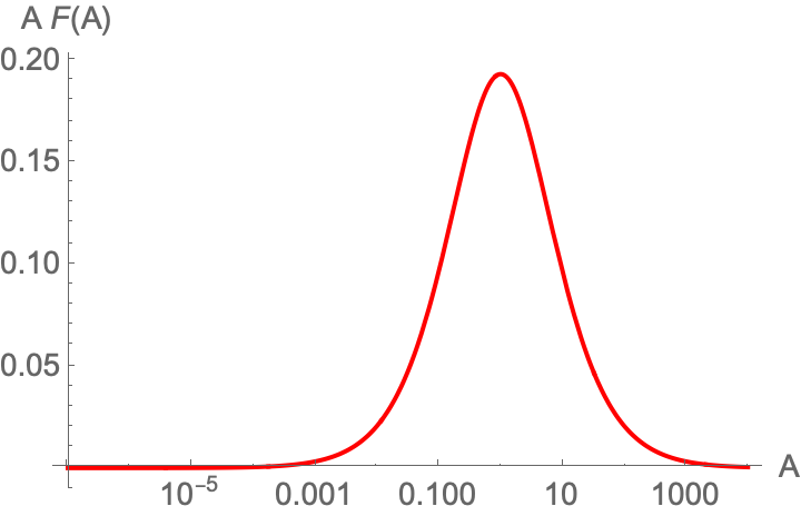
Figure 1: The function $A\,{\cal F}(A)$ defined in (40) that sets the scale of the backreaction.

III.6 Two-component fluids with increased backreaction

For baryons gravitationally coupled to cold dark matter, we had found in section  III.4 a truly minute backreaction of $O\left(10^{-13}\Omega_{B}\bar{\varepsilon}H\right)$. To what extent could backreaction in gravitationally coupled two-component fluids be larger if the material properties were different from those of standard baryonic matter?

III.6.1 Backreaction as a function of $c_{s}^{2}$ for $c_{s}^{2}\,a={\rm const.}$

To address this question, let us consider first a two-component system of the kind described in section  III.4, but where the sound velocity $c_{s}^{2}$ of the pressure-full matter component takes a value different from that of the baryonic fluid. Since the backreaction $D$ in (30) is proportional to $c_{s}^{2}$, one may try to increase the backreaction $D$ by increasing $c_{s}^{2}$. However, there is a tight upper bound to any such effort: the amplitude $\xi$ of the growing mode in (35) is reduced by increasing $c_{s}^{2}$. This reduction is larger for higher wavenumber $q$ and it thus regulates the integral (37) that determines $D$. The resulting $c_{s}^{2}$-dependence of $D$ is encoded in the dependence of the factor $A\,{\cal F}(A)$ in (39). Plotting this factor in Fig. 1, we see that backreaction reaches its maximum for $A\approx 1$ which corresponds to $c_{s}^{2}\,a=4\cdot 10^{-4}$ and that it decreases for larger $c_{s}^{2}$. The value $c_{s}^{2}\,a=4\cdot 10^{-4}$ still lies within the range of validity of our approximation scheme ($c_{s}^{2}\ll 1$) in which only terms proportional to $c_{s}^{2}k^{2}$ were kept.

For the baryonic fluid, we had determined $A\,{\cal F}(A)=8.1\cdot 10^{-9}$. According to Fig. 1, ${\rm max}\left[A\,{\cal F}(A)\right]=0.2$ is a factor $2.5\cdot 10^{7}$ larger. Therefore, a dark matter component with minimal pressure ($c_{s}^{2}\ll 1$) that couples gravitationally to cold dark matter and that participates in the growth of large scale structure with standard growing mode could exhibit a backreaction term as large as

$$D\approx 10^{-6}\,\Omega_{D}\bar{\varepsilon}H\,a\,.$$ (46)

While this is much larger than the value (41) obtained for the baryonic fluid, it still falls short of being detectable.

III.6.2 Backreaction for pressure and viscosity with arbitrary scale dependence

So far, we have considered only dark matter components which exhibit negligible viscosity and whose sound velocity has a particular $a$-dependence $c_{s}^{2}\,a={\rm const}$. We next ask to what extent other material properties could yield backreactions that are even larger than eq. (46). To this end, we explore now cosmological two-component fluids in which one of the two components shows material properties of arbitrary scale $\kappa_{s}$, $\kappa_{\eta}$ and with arbitrary power-law scale-dependence

$$c^{2}_{s}a = \kappa_{s}a^{\nu_{s}}\,,$$ (47)

$$c^{2}_{\eta}a=\frac{4}{3}\frac{\eta{\cal H}}{\bar{\varepsilon}} = \kappa_{\eta}a^{\nu_{\eta}}\,.$$ (48)

We introduce the shorthands $\phi_{i}\equiv\frac{\phi_{in}}{a_{in}}{\tilde{\phi}}_{i}$ for $i=1,2,3,4$. Eqs. (23)-(26) can be cast into two second-order differential equations for the growth of the density contrasts ${\tilde{\phi}}_{1}$ and ${\tilde{\phi}}_{3}$,

$$a^{2}\frac{d^{2}{\tilde{\phi}}_{1}}{da^{2}}+\left(\frac{3}{2}+\kappa_{\eta}{\tilde{k}}^{2}a^{\nu_{\eta}}\right)a\frac{d{\tilde{\phi}}_{1}}{da}$$ (49)

$$-\left(\frac{3}{2}\Omega_{D}-\kappa_{s}{\tilde{k}}^{2}a^{\nu_{s}}\right){\tilde{\phi}}_{1} = \frac{3}{2}(1-\Omega_{D}){\tilde{\phi}}_{3}\,,$$

$$a^{2}\frac{d^{2}{\tilde{\phi}}_{3}}{da^{2}}+\frac{3}{2}a\frac{d{\tilde{\phi}}_{3}}{da}-\frac{3}{2}(1-\Omega_{D}){\tilde{\phi}}_{3} = \frac{3}{2}\Omega_{D}{\tilde{\phi}}_{1}\,.$$ (50)

We consider again the case $\Omega_{D}\ll 1$ in which the growing mode is (almost) unperturbed. In the limit $\Omega_{D}\to 0$, eq. (50) has the solution ${\tilde{\phi}}_{3}=a$, so that eq. (49) becomes

$$a^{2}\frac{d^{2}{\tilde{\phi}}_{1}}{da^{2}}+\left(\frac{3}{2}+\kappa_{\eta}{\tilde{k}}^{2}a^{\nu_{\eta}}\right)a\frac{d{\tilde{\phi}}_{1}}{da}+\kappa_{s}{\tilde{k}}^{2}a^{\nu_{s}}{\tilde{\phi}}_{1}=\frac{3}{2}a.$$ (51)

For the viscosity-free case ($\kappa_{\eta}=0$) with constant $c_{s}^{2}a$ (i.e. $\nu_{s}=0$), the solution ${\tilde{\phi}}_{1}=\xi\,a$ of this equation reduces to eq.  (35). A numerical solution of the general case (51) is possible. We find it more instructive, however, to consider two special cases that illustrate the generic properties of the solution.

Case I: $\kappa_{s}=0$, $\kappa_{\eta}=$ finite. For this case, it is convenient to use the evolution equation ${\tilde{\phi}}_{2}={\tilde{\phi}}^{\prime}_{1}=a\,d{\tilde{\phi}}_{1}/da$ and to rewrite eq. (51),

$$a\frac{d{\tilde{\phi}}_{2}}{da}+\frac{1}{2}{\tilde{\phi}}_{2}+\kappa_{\eta}{\tilde{k}}^{2}a^{\nu_{\eta}}{\tilde{\phi}}_{2}=\frac{3}{2}a.$$ (52)

The solution is

$${\tilde{\phi}}_{2}(a)=e^{\frac{\kappa_{\eta}{\tilde{k}}^{2}}{\nu_{\eta}}(a_{i}^{\nu_{\eta}}-a^{\nu_{\eta}})}\sqrt{\frac{a_{i}}{a}}{\tilde{\phi}}_{2i}$$ (53)

$$\quad+\frac{3}{2\nu_{\eta}}a^{-\frac{1}{2}}\left(-\frac{\nu_{\eta}}{\kappa_{\eta}{\tilde{k}}^{2}}\right)^{\frac{3}{2\nu_{\eta}}}e^{-\frac{\kappa_{\eta}{\tilde{k}}^{2}}{\nu_{\eta}}a^{\nu_{\eta}}}$$

$$\quad\times\left(\Gamma\left[\frac{3}{2\nu_{\eta}},-\frac{\kappa_{\eta}{\tilde{k}}^{2}a_{i}^{\nu_{\eta}}}{\nu_{\eta}}\right]-\Gamma\left[\frac{3}{2\nu_{\eta}},-\frac{4\kappa_{\eta}{\tilde{k}}^{2}a^{\nu_{\eta}}}{\nu_{\eta}}\right]\right).$$

The first term in the above expression can be neglected for ${\tilde{\phi}}_{2i}=a_{i}\ll 1$. For $\nu_{\eta}>0$, a useful approximate solution can be obtained if one observes that the evolution is characterized by two regimes. During the early evolution, for small $a$, the last term in the rhs of eq. (52) is negligible and the solution is ${\tilde{\phi}}_{2}=a$. At late times, for $a\sim 1$, this last term becomes dominant and the solution is ${\tilde{\phi}}_{2}\simeq 3a^{1-\nu_{\eta}}/(2\kappa_{\eta}{\tilde{k}}^{2})$. A good fit of both regimes, giving also the correct order of magnitude for the short intermediate region, is given by the relation

$${\tilde{\phi}}_{2}(a)=\frac{a}{1+\frac{2}{3}\kappa_{\eta}{\tilde{k}}^{2}a^{\nu_{\eta}}}.$$ (54)

Case II: $\kappa_{\eta}=0$, $\kappa_{s}=$ finite. For this case the analytical solution is complicated and not very useful because of the presence of strong oscillations for large ${\tilde{k}}$. However, if one averages over the oscillations, the average field $\langle{\tilde{\phi}}_{1}\rangle$ can be described by a simple expression. In analogy with the viscous case, for small $a$, the solution is ${\tilde{\phi}}_{1}=a$, while for $a\sim 1$, the last term in the rhs of the averaged eq. (51) dominates and $\langle{\tilde{\phi}}_{1}\rangle\simeq 3a^{1-\nu_{v}}/(2\kappa_{s}{\tilde{k}}^{2})$. For $\nu_{s}>0$, a relation of sufficient accuracy for our purposes is

$$\langle{\tilde{\phi}}_{1}\rangle(a)=\frac{a}{1+\frac{2}{3}\kappa_{s}{\tilde{k}}^{2}a^{\nu_{s}}}.$$ (55)

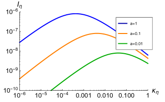
Figure 2: The integral $I_{\eta}$ in (56) determines the relative size of backreaction for a viscous dark matter component in units of $\Omega_{D}\bar{\varepsilon}H$. The plot is obtained for $c^{2}_{\eta}=\kappa_{\eta}a^{{\nu_{\eta}}-1}$ with ${\nu_{\eta}}=1$.

III.6.3 Numerical Results

The denominators of (54) and (55) are scale-dependent generalizations of the factor $\xi$ in (35) that regulates the UV-divergence of the integral over the power spectrum (37). In close analogy to the discussion in subsection III.6.1, this limits the possible growth of backreaction with pressure or viscosity. To be specific, let us consider for the case I the integral that determines the viscous contribution to the backreaction in (30),

$$I_{\eta}(\kappa_{\eta}) \equiv \int d^{3}q\,c^{2}_{\eta}\,P_{{\phi_{2}}{\phi_{2}}}(q)$$ (56)

$$= \kappa_{\eta}a^{\nu_{\eta}-1}\int d^{3}q\frac{P_{dd}(q)}{\left(1+\frac{2}{3}\kappa_{\eta}\tfrac{q^{2}}{{\cal H}_{0}^{2}}a^{\nu_{\eta}}\right)^{2}}$$

$$= \left(6\pi{\cal N}{\cal H}_{0}^{2}{\bar{q}}_{eq}\right)a\,C\,{\cal F}(C)\,.$$

Here, the prefactor $6\pi{\cal N}{\cal H}_{0}^{2}q_{eq}=4.2\cdot 10^{-6}$ is the same as in (39), and the solution $\propto C\,{\cal F}(C)$ of the integral is of the same functional form as (39), but with the $a$-dependent argument

$$C=\frac{2}{3}\kappa_{\eta}\tfrac{q_{eq}^{2}}{{\cal H}_{0}^{2}}a^{\nu_{\eta}}\,.$$ (57)

We know from Fig. 1 that ${\rm max}\left[C\,{\cal F}(C)\right]\approx 0.2$ and therefore, the viscous backreaction in (30) has a tight upper bound

$$D=\Omega_{D}\bar{\varepsilon}H\,I_{\eta}\leq 10^{-6}\Omega_{D}\bar{\varepsilon}H\,a$$ (58)

for the entire class of two-component fluid models considered here. This is consistent with the $\kappa_{\eta}$-dependence of $I_{\eta}$ plotted in Fig. 2.

We finally write the corresponding contribution to the backreaction (30) for the case II when viscosity vanishes but sound velocity has an arbitrary $a$-dependence, $c^{2}_{s}\sim a^{\nu_{s}-1}$.

$$I_{s}(\kappa_{s})\equiv\int d^{3}q\,c^{2}_{s}\,P_{{\phi_{1}}{\phi_{2}}}(q)$$

$$\quad=\kappa_{s}a^{{\nu_{s}}-1}\int d^{3}q\frac{1+\frac{2}{3}(1-\nu_{s})\tfrac{q^{2}}{{\cal H}_{0}^{2}}\kappa_{s}\,a^{\nu_{s}}}{\left(1+\frac{2}{3}\tfrac{q^{2}}{{\cal H}_{0}^{2}}\kappa_{s}a^{\nu_{s}}\right)^{3}}{P}_{dd}(q)\,.\qquad$$ (59)

While this integral differs somewhat from (56), the UV-cut on the spectrum ${P}_{dd}(q)$ is set by a similar $q$-dependent denominator. This explains why the numerical evaluation of (59) in Fig. 3 yields also in this case a tight upper bound of the backreaction $D\leq O(10^{-6})\Omega_{D}\bar{\varepsilon}H\,a$.

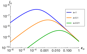
Figure 3: The integral $I_{s}$ in (59) determines in units of $\Omega_{D}\bar{\varepsilon}H$ the relative size of backreaction for a dark matter component with sound velocity $c^{2}_{s}=\kappa_{s}a^{{\nu_{s}}-1}$. The plot is for ${\nu_{s}}=1$.

IV Backreaction for cosmological matter beyond the linear fluid approximation

Our discussion so far was based on describing matter in terms of ideal or Navier-Stokes fluid dynamics, and on following only scalar perturbations that were assumed to propagate in a linear way. These assumptions become questionable at late times and on small scales when cosmological structure formation becomes non-linear. Here, we provide a formulation of backreaction that remains valid beyond this linearized fluid-dynamic regime and that reduces to the formalism of section III in the limit in which Navier-Stokes fluid dynamics applies.

The need to go beyond a fluid dynamic formulation is particularly clear for the modelling of cold dark matter at late times and sufficiently small scales. At early times and very large scales, CDM is well-described by the single stream approximation which is equivalent to a description in terms of an ideal and pressure-less fluid. At late times, however, deviations from local equilibrium grow large, and the velocity dispersion induced by shell crossing modifies the dynamics Pueblas:2008uv ; Hahn:2014lca ; Erschfeld:2018zqg . In addition to scalar perturbations, also vector perturbations (e. g. vorticity) are generated by non-linear terms. Also the effect of dark matter self-interactions would show up in this regime. At even smaller scales, our current understanding of cosmological evolution is incomplete.

To understand cosmological evolution, we are particularly interested in the energy density $\varepsilon(x)$. In a particle picture, it receives contributions from rest masses, from interactions and from the kinetic motion of particles (internal energy). For a one-component fluid with a single (at least approximately) conserved particle quantum number, the differential of this energy density is

$$d\varepsilon=Tds+\mu dn\,,$$ (60)

with temperature $T$, entropy density $s$, chemical potential $\mu$ and particle density $n$. Eq. (60) holds even if the fluid evolution is highly non-linear or turbulent and can be seen as a definition of $T$ and $\mu$. Such more general dynamical scenarios also allow for the definition of an entropy current $s^{\mu}$, as well as a particle number current $N^{\mu}$, so that one can write

$$s^{\mu}=su^{\mu}+\frac{1}{T}q^{\mu}-\frac{\mu}{T}\nu^{\mu},\quad\quad\quad N^{\mu}=nu^{\mu}+\nu^{\mu},$$ (61)

with fluid velocity $u^{\mu}$, heat current $q^{\mu}$ and diffusion current $\nu^{\mu}$. The heat current $q^{\mu}$ and diffusion current $\nu^{\mu}$ are orthogonal to the fluid velocity, $u_{\mu}q^{\mu}=u_{\mu}\nu^{\mu}=0$. Depending on the precise definition of the fluid velocity, there is an additional relation for $q^{\mu}$ and $\nu^{\mu}$ (e.g., $q^{\mu}=0$ in the Landau frame or $\nu^{\mu}=0$ in the Eckart frame), but we keep this frame definition open.

Combining eqs. (60) and (61) and using $\varepsilon+p=Ts+\mu n$, we obtain

$$u^{\mu}\partial_{\mu}\varepsilon+(\varepsilon+p)\nabla_{\mu}u^{\mu}=\tilde{\sigma}\,,$$ (62)

with

$$\tilde{\sigma}=T\nabla_{\rho}(s^{\rho}-q^{\rho}/T)+\mu\nabla_{\rho}N^{\rho}+T\nu^{\rho}\partial_{\rho}(\mu/T)\,.$$ (63)

Entropy production $\nabla_{\rho}s^{\rho}$ and the change $\nabla_{\rho}N^{\rho}$ of particle number vanish in global equilibrium, and so does the heat current $q^{\mu}$ and the diffusion current $\nu^{\mu}$. Therefore, the term $\tilde{\sigma}$ is proportional to gradients and it vanishes in equilibrium or for an ideal fluid.

Amongst all possibilities for gradient terms to contribute to (62), the combination $\nabla_{\mu}u^{\mu}$ is distinguished in the cosmological context, because it is non-vanishing already for a homogeneous and isotropic fluid with Hubble expansion. We define therefore

$$\sigma=\tilde{\sigma}+\pi_{\text{bulk}}\nabla_{\mu}u^{\mu},$$ (64)

where $\pi_{\text{bulk}}$ is defined such that $\sigma$ vanishes for a homogeneous and isotropic but expanding or contracting fluid. Alternatively, and equivalently, it is defined through the tensor decomposition of the energy-momentum tensor with respect to the fluid velocity $u^{\mu}$,

$$T^{\mu\nu}=\varepsilon u^{\mu}u^{\nu}+(p+\pi_{\text{bulk}})\Delta^{\mu\nu}+\pi^{\mu\nu}+q^{\mu}u^{\nu}+u^{\mu}q^{\nu}.$$ (65)

Eq. (62) becomes then

$$u^{\mu}\partial_{\mu}\varepsilon+(\varepsilon+p+\pi_{\text{bulk}})\nabla_{\mu}u^{\mu}=\sigma.$$ (66)

By construction, the right hand side of eq. (66) vanishes for a homogeneous and isotropic fluid with FLRW expansion. In that case, eq. (66) gives the standard energy conservation law. However, for an inhomogeneous fluid for which homogeneity and isotropy are only symmetries in a statistical sense, the right hand side of eq. (66) can be, and will be, non-vanishing, for example due to terms quadratic in perturbations.

Assuming that metric perturbations are negligible, we can rewrite eq. (66) in terms of deviations $\vec{v}$ from the local Hubble flow. Using $u^{\mu}=(\gamma,\gamma\vec{v})$, $\gamma=1/a\sqrt{1-\vec{v}^{2}}$, we find

$$\begin{split}&\dot{\varepsilon}+\vec{v}\cdot\vec{\nabla}\varepsilon+(\varepsilon+p+\pi_{\text{bulk}})\left(3\frac{\dot{a}}{a}+\vec{\nabla}\cdot\vec{v}\right)=\frac{\sigma}{\gamma}.\end{split}$$ (67)

As the combination $\vec{v}\cdot\vec{\nabla}\varepsilon+\varepsilon\,\vec{\nabla}\cdot\vec{v}$ is a total derivative with vanishing spatial average, the spatial average of eq. (67) reads

$$\frac{1}{a}\dot{\bar{\varepsilon}}+3H\,(\bar{\varepsilon}+\bar{p}+\bar{\pi}_{\text{bulk}})=D\,,$$ (68)

where

$$D=\frac{1}{a}\langle\vec{v}\cdot\vec{\nabla}(p+\pi_{\text{bulk}})\rangle+\left\langle\sigma\sqrt{1-\vec{v}^{2}}\right\rangle.$$ (69)

We stress again that $D$ vanishes by construction in an exactly homogeneous and isotropic universe and that it starts quadratically in fluctuations. The form of (69) is more general than the derivation given in Ref. Floerchinger:2014jsa and used in section III, since it does not assume that the fluctuations are small or that $D$ is dominated by terms that are second order in fluctuations. For illustration, we consider some special cases for this general formula:

• For an ideal fluid with pressure one has $\sigma=\pi_{\text{bulk}}=0$, and

  $$D=-\frac{1}{a}\langle\delta p\,\vec{\nabla}\cdot\vec{v}\rangle.$$ (70)

  This is the case of our illustrative introductory example (7) that describes a modification of energy density due to work done in an imhomogeneous fluid by contraction against local pressure gradients. In Fourier-space, $\delta p(x)=\int d^{3}q\,{\delta p}(q)e^{iqx}$, it can be written as an integral over the power spectrum $D=-\frac{1}{a}\int d^{3}qP_{\theta p}(\vec{q})$, which is the first term of (5).

• In a first order gradient expansion (Navier-Stokes approximation) in the Landau frame one has $q^{\rho}=0$ and the local entropy production

  $$\quad\quad\nabla_{\mu}s^{\mu}=-\tfrac{1}{T}\left[\pi_{\text{bulk}}\nabla_{\alpha}u^{\alpha}+\pi^{\alpha\beta}\nabla_{\alpha}u_{\beta}\right]-\nu^{\alpha}\partial_{\alpha}(\tfrac{\mu}{T}).$$ (71)

  For $\nabla_{\mu}N^{\mu}=0$, this leads to the simple expression

  $$\sigma=-\pi^{\alpha\beta}\nabla_{\alpha}u_{\beta}.$$ (72)

  For exactly homogeneous and isotropic fields without inhomogeneities but with FLRW expansion, the only non-vanishing term in $\langle\nabla_{\mu}s^{\mu}\rangle$ is proportional to the spatially averaged bulk viscous pressure

  $$\bar{\pi}_{\text{bulk}}=-3\bar{\zeta}H\,.$$ (73)

  According to the definition (64), this term cancels in $\sigma$ and therefore $D=0$ in the absence of inhomogeneities. However, (73) appears also on the left hand side of (68). The resulting bulk viscous cosmologies without inhomogeneities have received much attention in model studies Murphy:1973zz ; Belinskii ; Padmanabhan:1987dg ; Fabris:2005ts ; Wilson:2006gf ; Colistete:2007xi ; Mathews:2008hk ; Li:2009mf ; Velten:2011bg ; Gagnon:2011id .

  Keeping in (71) terms up to second order in inhomogeneities, one recovers the dissipative terms derived in Floerchinger:2014jsa and given in the second and third line of eq. (5),

  $$D = \frac{1}{a^{2}}\left(\bar{\zeta}+\frac{4}{3}\bar{\eta}\right)\int d^{3}qP_{\theta\theta}(\vec{q})$$ (74)

  $$+\frac{1}{a^{2}}\bar{\eta}\int d^{3}q\left(P_{w}\right)_{jj}(\vec{q})\,.$$

  These terms correspond to the contribution to energy evolution from the entropy production (dissipation) in fluid velocity perturbations.

• The backreaction term $D$ in eq. (69) can also be evaluated in far-from-equilibrium situations. One particularly explicit example is given by a system without conserved particle number, $N^{\mu}=0$, in the Landau frame $q^{\mu}=0$, when (63) reduces to

  $$\tilde{\sigma}=T\nabla_{\rho}s^{\rho}\,.$$ (75)

  In this case, the term $\left\langle\sigma\sqrt{1-\vec{v}^{2}}\right\rangle$ in (69) is the spatial average over local entropy production times temperature and an inverse gamma-factor. In any kinetic theory description, even far-from-equilibrium, local entropy production $\nabla_{\rho}s^{\rho}\geq 0$ follows from Boltzmann’s $H$-theorem and is non-vanishing as a result of collisions away from detailed balance. By working in kinetic theory, or in non-equilibrium quantum field theory, one can therefore evaluate $D$ beyond the simple first-order fluid approximation entering eq. (5).

• From the decomposition (65) and the covariant conservation law $\nabla_{\mu}T^{\mu\nu}=0$, one obtains the alternative relation

  $$\sigma=-\pi^{\alpha\beta}\nabla_{\alpha}u_{\beta}-\nabla_{\alpha}q^{\alpha}+u_{\beta}u^{\alpha}\nabla_{\alpha}q^{\beta}.$$ (76)

  This is formulated in terms of the energy-momentum tensor only and it does not make reference to entropy. For any form of out-of-equilibrium dynamics that follows the energy momentum tensor and that associates local flow fields (such as e.g. a kinetic theory formulation), all terms entering (76) are then given.

• Relaxing covariant particle number conservation, $\nabla_{\mu}N^{\mu}\geq 0$, eq. (69) allows for an increase in the energy density by backreaction involving inelastic processes.

These remarks illustrate the general point that working within the framework of a fluid-dynamic evolution with linearized treatment of inhomogeneities does not exhaust scenarios in which backreaction can occur. We would find it particularly interesting to understand whether increased backreaction effects can be realized in far-from-equilibrium scenarios that are accompanied by significant entropy production or significant violations of particle number conservation.

V Conclusions

This work analysed the combined evolution equations for the homogeneous part of the cosmological energy density and the growth of inhomogeneities, accounting for backreaction from the latter to the former. The evolution equations for the spatial averages (see eqs. (1) and (67)) and for the linearized inhomogeneities (see eqs. (8) to (11)) combine to a set of integro-differential equations that are difficult to solve in general. However, for perturbatively small inhomogeneities, one can solve the linearized evolution equation for perturbations in the absence of backreaction, and then determine the backreaction from the solutions. Based on this approximation, we gave in the present paper novel, explicit and compact expressions for how backreaction modifies Friedmann’s equation in late-time cosmology.

A basic conclusion that can be drawn is that backreaction on the cosmological evolution is not necessarily linked to large metric perturbations, such as (Post-) Newtonian potentials. The original proposal of Ref. Floerchinger:2014jsa had already emphasized this point. We discussed here an explicit realization, which has the appealing property that it makes use of two fundamental ingredients of the cosmological model: baryonic and dark matter. In section III we saw that the growth of structure proceeds in the gravitationally coupled systems of baryons and dark matter, despite the pressure that develops in the baryonic sector because of the small amount of ionization that it retains even after recombination. The simultaneous presence of pressure and significant structure growth makes the first contribution to the backreaction term of eq. (5) nonvanishing. The second important conclusion is that the sign of the backreaction term is such that the effect leads to the enhancement of the averaged energy density that drives the expansion. For backreaction through pressure this growth arises through the work done against perturbations. A similar conclusion can be reached for the backreaction through viscosity.

In the above example, the known baryon sound velocity is too small for the effect to be detectable. Replacing baryons by a hypothetical second dark-matter sector with nonzero pressure or viscosity enlarges the parameter range and leads to the enhancement of the effect by several orders of magnitude. However, the standard cosmological expansion is still not modified significantly. The analysis of section III reveals the reason by providing a refined general picture of what limits the maximal size of backreaction effects from inhomogeneities of matter fields. The backreaction terms in eq. (5) are integrals over measured or measurable power spectra. They are multiplied by the velocity of sound or by a viscous transport coefficient respectively. One may thus have expected that the maximal size of backreaction is set by the current phenomenological constraints on warm dark matter or viscous matter. But this is not the case. The growth of large scale structure is certainly known to put significant constraints on non-ideal fluid alternatives to CDM, but our choice of non-ideal fluids gravitationally coupled to CDM was designed to evade possible constraints from LSS. In doing so, we have encountered an even tighter and more generic constraint: any pressure or viscous correction gives rise to a physical UV-cut-off of the (logarithmically divergent) integral over the power spectrum that determines backreaction, see eq. (37), (56) and (29). This reduces backreaction below the conceivably detectable level for arbitrary choices of sound velocity or viscosity.

The analysis in section III has concentrated on cosmological times and regimes of scales where the evolution of inhomogeneities is close to linear. This allowed to make progress with analytical methods, but also implies – almost by construction – that backreaction terms remain small (and perturbation theory remains consistent). On the other side it is also clear that cosmological perturbation theory breaks down at late times and on small scales. The evolution of matter fields is then modified for example by the generation of velocity dispersion generated by stream crossing, or by non-linear terms in the evolution equations for scalar perturbations. Also vector and even tensor perturbations, like vorticity or shear stress, are generated by non-linear terms and can play an interesting role at small scales. Dark-matter self-interactions could modify the dynamics in the non-linear regime as well. Backreaction terms can be written as integrals over equal-time power spectra of inhomogeneities, and it is well possible that these integrals are dominated by small scales where non-linear effects are large. It would therefore be particularly interesting to extend our analysis into that regime. Of course this is technically challenging and needs a good understanding of non-linear physics.

In order to prepare for a future extension into the non-linear and out-of-equilibrium regime, we have formulated the backreaction terms for the evolution of energy density in very general terms in section IV. This new formulation does not rely on the Navier-Stokes fluid approximation and can also be applied for example in the context of far-from-equilibrium quantum field or kinetic theory. It would be interesting to establish in the future an understanding of backreaction effects from the non-linear regime of matter field inhomogeneities to the overall cosmological expansion.

Appendix A Further remarks on the modified Friedmann equation

In this appendix, we further explore general consequences of the modified Friedmann equation (II). To this end, we first define the critical total energy density $\bar{\varepsilon}_{c}$ by

$$H^{2}=\frac{8\pi G_{\text{N}}}{3}\left[\bar{\varepsilon}_{c}-\int_{\tau_{\text{I}}}^{\tau}d\tau^{\prime}\left(\frac{a(\tau^{\prime})}{a(\tau)}\right)^{4}a(\tau^{\prime})D(\tau^{\prime})\right].$$ (77)

When the integral over $D$ is positive, the total average energy density today $\bar{\varepsilon}_{0,c}$, for vanishing spatial curvature, is larger than the value usually taken for the critical energy density,

$$\bar{\varepsilon}_{0,c}>\frac{3H_{0}^{2}}{8\pi G_{\text{N}}}.$$ (78)

If the dissipative term $D$ is non-zero during some time interval, a part of the total background energy density $\bar{\varepsilon}_{c}$ has been produced by dissipative processes. It might be useful to separate that part and to decompose the total background energy density additively as

$$\bar{\varepsilon}_{c}=\bar{\varepsilon}+\bar{\varepsilon}_{D}$$ (79)

where $\bar{\varepsilon}$ is the conventional contribution of matter and radiation that does not result from backreaction and $\bar{\varepsilon}_{D}$ is the part of the internal energy that results from the dissipation of perturbations. The part $\bar{\varepsilon}_{D}$ has the evolution

$$\dot{\bar{\varepsilon}}_{D}+3\frac{\dot{a}}{a}(\bar{\varepsilon}_{D}+\bar{p}_{D}+\bar{\pi}_{\text{bulk},D})=aD,$$ (80)

for suitably defined pressure $\bar{p}_{D}$ and bulk viscous pressure $\bar{\pi}_{\text{bulk},D}$. We assume now for simplicity the relation

$$\bar{p}_{D}+\bar{\pi}_{\text{bulk},D}=\hat{w}_{D}\,\bar{\varepsilon}_{D},$$ (81)

where $\hat{w}_{D}$ is some constant. After integrating, one finds

$$\bar{\varepsilon}_{D}(\tau)=\int_{\tau_{\text{I}}}^{\tau}d\tau^{\prime}\left(\frac{a(\tau^{\prime})}{a(\tau)}\right)^{3+3\hat{w}_{D}}a(\tau^{\prime})D(\tau^{\prime}).$$ (82)

Using this, as well as the decomposition (79) in the modified Friedmann equation yields

$$\begin{split}H(\tau)^{2}&=\frac{8\pi G_{\text{N}}}{3}{\bigg{[}}\bar{\varepsilon}(\tau)\\ &+\int_{\tau_{\text{I}}}^{\tau}d\tau^{\prime}\left[\left(\tfrac{a(\tau^{\prime})}{a(\tau)}\right)^{3+3\hat{w}_{D}}-\left(\tfrac{a(\tau^{\prime})}{a(\tau)}\right)^{4}\right]a(\tau^{\prime})D(\tau^{\prime}){\bigg{]}}.\end{split}$$ (83)

One first notes that one recovers the conventional Friedmann equation for $D(\tau^{\prime})=0$ or if $\hat{w}_{D}=1/3$. The latter condition would correspond to $\bar{\varepsilon}_{D}$ consisting of pure radiation. If $\hat{w}_{D}$ is smaller than $1/3$, the Friedmann equation is modified and in particular, today’s value of the energy density $\bar{\varepsilon}$ not produced by backreaction becomes

$$\begin{split}(\bar{\varepsilon})_{0}&=\frac{3H_{0}^{2}}{8\pi G_{\text{N}}}\\ &-\int_{\tau_{\text{I}}}^{\tau}d\tau^{\prime}\left[\left(\tfrac{a(\tau^{\prime})}{a(\tau)}\right)^{3+3\hat{w}_{\text{d}}}-\left(\tfrac{a(\tau^{\prime})}{a(\tau)}\right)^{4}\right]a(\tau^{\prime})D(\tau^{\prime}),\end{split}$$ (84)

which for $D>0$ is smaller than the conventional value because the integral is positive.

References

- (1) S. R. Green and R. M. Wald, “A simple, heuristic derivation of our ‘no backreaction’ results,” Class. Quant. Grav. 33 (2016) no.12, 125027 [arXiv:1601.06789 [gr-qc]].
- (2) T. Buchert, M. Carfora, G. F. R. Ellis, E. W. Kolb, M. A. H. MacCallum, J. J. Ostrowski, S. Räsänen, B. F. Roukema, L. Andersson and A. A. Coley, et al. “Is there proof that backreaction of inhomogeneities is irrelevant in cosmology?,” Class. Quant. Grav. 32 (2015), 215021 [arXiv:1505.07800 [gr-qc]].
- (3) T. Buchert and S. Räsänen, “Backreaction in late-time cosmology,” Ann. Rev. Nucl. Part. Sci. 62 (2012), 57-79 [arXiv:1112.5335 [astro-ph.CO]].
- (4) C. Wetterich, “Can structure formation influence the cosmological evolution?,” Phys. Rev. D 67, 043513 (2003) [astro-ph/0111166].
- (5) S. R. Green and R. M. Wald, “A new framework for analyzing the effects of small scale inhomogeneities in cosmology,” Phys. Rev. D 83, 084020 (2011) [arXiv:1011.4920 [gr-qc]].
- (6) S. Floerchinger, N. Tetradis and U. A. Wiedemann, “Accelerating Cosmological Expansion from Shear and Bulk Viscosity,” Phys. Rev. Lett. 114 (2015) no.9, 091301 [arXiv:1411.3280 [gr-qc]].
- (7) B. Li and J. D. Barrow, “Does Bulk Viscosity Create a Viable Unified Dark Matter Model?,” Phys. Rev. D 79 (2009) 103521 [arXiv:0902.3163 [gr-qc]].
- (8) H. Velten and D. J. Schwarz, “Constraints on dissipative unified dark matter,” JCAP 1109 (2011) 016 [arXiv:1107.1143 [astro-ph.CO]].
- (9) J. S. Gagnon and J. Lesgourgues, “Dark goo: Bulk viscosity as an alternative to dark energy,” JCAP 1109 (2011) 026 [arXiv:1107.1503 [astro-ph.CO]].
- (10) D. Blas, S. Floerchinger, M. Garny, N. Tetradis and U. A. Wiedemann, “Large scale structure from viscous dark matter,” JCAP 1511 (2015) 049 [arXiv:1507.06665 [astro-ph.CO]].
- (11) C. M. S. Barbosa, H. Velten, J. C. Fabris and R. O. Ramos, “Assessing the impact of bulk and shear viscosities on large scale structure formation,” Phys. Rev. D 96 (2017) no.2, 023527 doi:10.1103/PhysRevD.96.023527 [arXiv:1702.07040 [astro-ph.CO]].
- (12) S. Floerchinger, M. Garny, N. Tetradis and U. A. Wiedemann, “Renormalization-group flow of the effective action of cosmological large-scale structures,” JCAP 1701 (2017) 048 [arXiv:1607.03453 [astro-ph.CO]].
- (13) C. P. Ma and E. Bertschinger, “Cosmological perturbation theory in the synchronous and conformal Newtonian gauges,” Astrophys. J. 455 (1995), 7-25 doi:10.1086/176550 [arXiv:astro-ph/9506072 [astro-ph]].
- (14) S. Weinberg, “Cosmology,” Oxford, UK: Oxford Univ. Pr. (2008)
- (15) S. Pueblas and R. Scoccimarro, “Generation of Vorticity and Velocity Dispersion by Orbit Crossing,” Phys. Rev. D 80 (2009) 043504 [arXiv:0809.4606 [astro-ph]].
- (16) O. Hahn, R. E. Angulo and T. Abel, “The Properties of Cosmic Velocity Fields,” Mon. Not. Roy. Astron. Soc. 454 (2015) no.4, 3920 [arXiv:1404.2280 [astro-ph.CO]].
- (17) A. Erschfeld and S. Floerchinger, “Evolution of dark matter velocity dispersion,” JCAP 06 (2019), 039 doi:10.1088/1475-7516/2019/06/039 [arXiv:1812.06891 [astro-ph.CO]].
- (18) G. L. Murphy, “Big-bang model without singularities,” Phys. Rev. D 8 (1973) 4231.
- (19) V. A. Belinskii and I. M. Khalatnikov, “Influence of viscosity on the character of cosmological evolution,” Zh. Eksp. Teor. Fiz., 69:401, 1975 (Sov. Phys. JETP 42 (1976) 205).
- (20) T. Padmanabhan and S. M. Chitre, “Viscous universes,” Phys. Lett. A 120 (1987) 433.
- (21) J. C. Fabris, S. V. B. Goncalves and R. de Sa Ribeiro, “Bulk viscosity driving the acceleration of the Universe,” Gen. Rel. Grav. 38 (2006) 495 [astro-ph/0503362].
- (22) J. R. Wilson, G. J. Mathews and G. M. Fuller, “Bulk Viscosity, Decaying Dark Matter, and the Cosmic Acceleration,” Phys. Rev. D 75 (2007) 043521 [astro-ph/0609687].
- (23) R. Colistete, J. C. Fabris, J. Tossa and W. Zimdahl, “Bulk Viscous Cosmology,” Phys. Rev. D 76 (2007) 103516 [arXiv:0706.4086 [astro-ph]].
- (24) G. J. Mathews, N. Q. Lan and C. Kolda, “Late Decaying Dark Matter, Bulk Viscosity and the Cosmic Acceleration,” Phys. Rev. D 78 (2008) 043525 [arXiv:0801.0853 [astro-ph]].