Spatial Distribution of Distortion due to Nonlinear Power Amplification in Distributed Massive MIMO

Abstract

Due to the nonlinearity of power amplifiers (PAs), the transmit signal is distorted. Previous works have studied the spatial distribution of this distortion for a central massive multiple input multiple output (MIMO) array. In this work, we extend the analysis for distributed massive MIMO in a line-of-sight (LoS) scenario. We show that the distortion is not always uniformly distributed in space. In the single-user case, it coherently combines at the user location. In the few users case, the signals will add up at the user locations plus several others locations. As the number of users increases, it becomes close to uniformly distributed. As a comparison with a central massive MIMO system, having the same total number of antennas, the distortion in distributed massive MIMO is considerably more uniformly distributed in space. Moreover, the potential coherent combining is contained in a zone rather than in generic directions, i.e., in a beamspot. Furthermore, a small-scale fading effect is observed at unintended locations due to the non-coherent combining of the signals. As a result, one can expect that going towards distributed systems allows working closer to saturation, increasing the PA operating efficiency and/or using low-cost PAs.

I Introduction

Distributed and cell-free massive MIMO are prime candidates for next generation wireless systems thanks to their potential to offer consistent good service and increased and scalable capacity [1]. A highly energy efficient system can be realized provided the system can operate the PAs close to saturation. In this region however, they exhibit nonlinear behaviour generating distortion, both in-band (IB) and out-of-band (OOB).

The occurrence and impact of distortions due to nonlinear power amplification has been studied in literature for the case of central massive MIMO with one large central array at the basestation. When the distortions generated by the many PAs are assumed to be uncorrelated, it was shown that they do not combine coherently in space. Hence, thanks to the large number of transmit antennas, great performance and energy efficient operation can be achieved [2]. However, in general the distortion terms are correlated over the transmit antennas and they may significantly impact both the IB signal quality and the OOB radiation [3] under specific conditions. The spatial distribution of the distortion due to nonlinear power amplification has been rigorously studied for the case of massive MIMO central large array in [4]. The authors prove that in particular the transmission scenarios with one or few user equipments (UEs) that are in LoS to the basestation need to be considered. Indeed not only the wanted information signal for the intended UEs yet also the distortions may in this case get significant antenna array gain.

In this paper we study the spatial distribution of distortion due to nonlinear power amplification for distributed array deployments, as depicted in Fig. 1, and exemplary for cell-free massive MIMO. For simplicity and to gain insight we focus on relatively simple scenarios: antenna arrays with omnidirectional antennas and no coupling between them are considered, transmitting to a single-user or multiple users in LoS. We further show that the LoS conditions present a worst case in terms of detrimental combining of the distortion terms. Analytical expressions are derived for the case of a matched filtering (MF) beamformer and a general single-carrier formulation. We further comment on the expectations for more complex transmission scenarios.

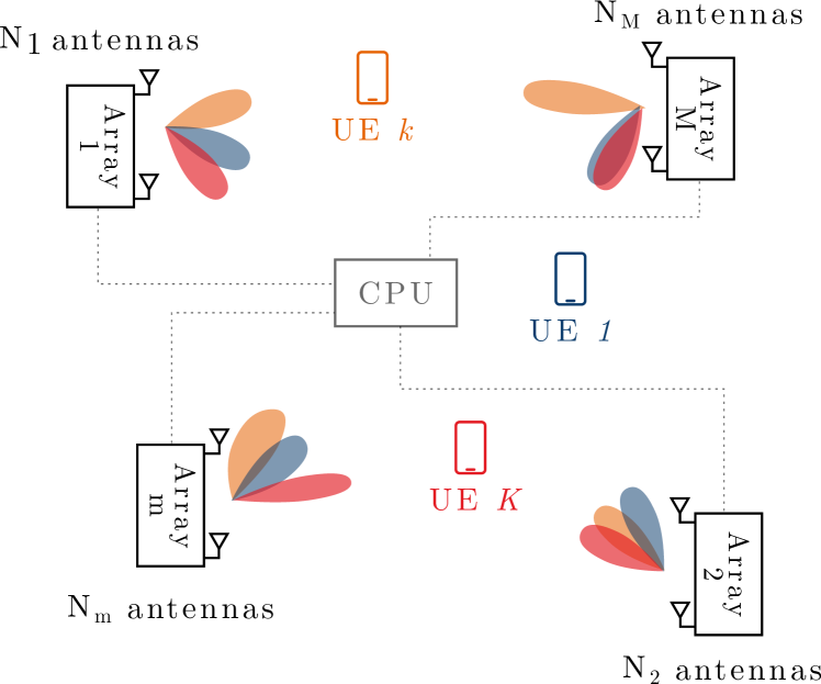
Figure 1: Distributed MIMO System with CPU, $K$ single-antenna users, $M$ arrays, each with $N_{m}$ antennas.

Notations: Superscript ^∗ stands for conjugate, $\jmath$ is the imaginary unit and $\mathbb{E}(.)$ is the expectation. $\circledast$ denotes the convolution. $\delta_{n}$ and $\delta(t)$ are the Kronecker and Dirac deltas respectively.

II System Model

II-A Signal Model

As shown in Fig. 1, we consider a distributed massive MIMO systems with a total of $M$ antenna arrays, perfectly synchronized with one another and with perfect channel state information. We denote the number of antennas of array $m$ as $N_{m}$. A total of $K$ single-antenna UEs are being served simultaneously using the same time and frequency resources. A conventional massive MIMO system with one large central array is obtained in the particular case $M=1$.

The complex baseband representation of the signal intended for UE $k$ is denoted by $s^{(k)}(t)$, for $k=1,...,K$. It is assumed to be wide sense stationary and uncorrelated between different users. They have the same power spectral density (PSD) $S(\omega)$, with a power scaling $p^{(k)}$. We define the inverse Fourier transform of $S(\omega)$ as $R(\tau)$. The cross-correlation and cross-PSD of the transmit signals are then given by

$${R}_{s^{(k)}s^{(k^{\prime})}}(\tau) =\mathbb{E}\left(s^{(k)}(t+\tau)(s^{(k^{\prime})}(t))^{*}\right)=\delta_{k-k^{\prime}}p^{(k)}R(\tau)$$

$$S_{s^{(k)}s^{(k^{\prime})}}(\omega) =\delta_{k-k^{\prime}}p^{(k)}S(\omega),$$ (1)

where we used the fact that user signals are uncorrelated. The transmitter structure of array $m$ is shown in Fig. 2. The signal $s^{(k)}(t)$ is precoded at transmit antenna $n$ of array $m$ using a filter $w_{m,n}^{(k)}(t)$. The complex baseband representation of the signal before the PA of the corresponding antenna is denoted by $x_{m,n}(t)$ and is given by

$$x_{m,n}(t)=\sum_{k=1}^{K}s^{(k)}(t)\circledast w_{m,n}^{(k)}(t).$$ (2)

II-B Nonlinear PA Model

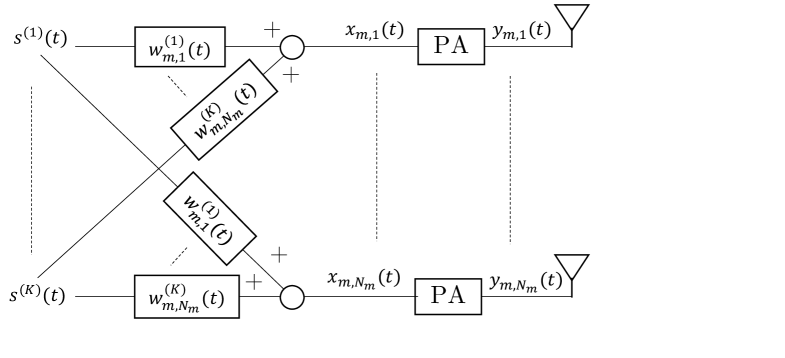
Figure 2: Transmitter structure of array $m$ with $N_{m}$ antennas.

Keeping only terms that appear around the carrier frequency, the baseband representation of the signal after the PA can generally be written as [5, 4]

$$y_{m,n}(t)=\sum_{l=1,3,5,...}b_{l}x_{m,n}(t)|x_{m,n}(t)|^{l-1}.$$ (3)

The first order term ($l=1$) will be referred to as the useful signal part, while the sum of the higher order terms will be referred to as distortion. Note that distortion is present both in-band and out-of-band. We define the cross-correlations of the signals $x_{m,n}(t)$ and $y_{m,n}(t)$ (before and after the PA) as ${R}_{{x}_{m,n}{x}_{m^{\prime},n^{\prime}}}(\tau)$ and ${R}_{{y}_{m,n}{y}_{m^{\prime},n^{\prime}}}(\tau)$ respectively. As in [4], we assume that the complex baseband signal $x_{m,n}(t)$ can be modeled as a zero mean circularly symmetric Gaussian random variable. This is particularly true if the signal is beamformed and OFDM modulated. Then, we can use the result of [4, 6] to relate the cross-antenna correlation of the input of the PA to the one at the output of the PA

$${R}_{{y}_{m,n}{y}_{m^{\prime},n^{\prime}}}(\tau)$$ (4)

$$=\sum_{l=1,3,5,...}c_{l}{R}_{{x}_{m,n}{x}_{m^{\prime},n^{\prime}}}(\tau)|{R}_{{x}_{m,n}{x}_{m^{\prime},n^{\prime}}}(\tau)|^{l-1},$$

where $n$ and $n^{\prime}$ are antenna indices of array $m$ and $m^{\prime}$ respectively. Coefficients $c_{l}$ can be related to $b_{l}$ and the input power of each PA [4].

II-C Channel Model

The channel from each array to a given location is assumed in pure LoS with no other multipath components, and in the far field from each array. This location could be either a UE or an observer location. Considering omnidirectional antennas and uniform linear arrays (ULAs), the baseband representation of the channel impulse response between the given location and antenna $n$ of array $m$ is

$${h}_{m,n}(t) =\beta_{m}\delta(t-\tau_{m})e^{-\jmath\phi_{m}n}.$$

The delay $\tau_{m}$ accounts for the propagation delay between array $m$ and the given location. The complex coefficient $\beta_{m}=|\beta_{m}|e^{-\jmath\psi_{m}}$, models the path loss between array $m$ and the given location together with a phase shift $\psi_{m}=2\pi f_{c}\tau_{m}$. Finally, the complex exponential $e^{-\jmath\phi_{m}n}$ accounts for the phase shift of antenna $m$ with respect to reference antenna $n=0$, with $\phi_{m}=\frac{2\pi}{\lambda_{c}}d\cos(\theta_{m})$, where $\lambda_{c}$ the carrier wavelength, $d$ the inter-antenna spacing and $\theta_{m}$ the angular direction of the given location with respect to array $m$. Moreover, we define the channel between the UE $k$ and antenna $n$ of array $m$ as

$${h}_{m,n}^{(k)}(t) =\beta_{m}^{(k)}\delta(t-\tau_{m}^{(k)})e^{-\jmath\phi_{m}^{(k)}n}.$$

The received signal at the considered location is given by

$$r(t) =\sum_{m=1}^{M}\sum_{n=0}^{N_{m}-1}{y}_{m,n}(t)\circledast{h}_{m,n}(t)$$

$$=\sum_{m=1}^{M}\beta_{m}\sum_{n=0}^{N_{m}-1}{y}_{m,n}(t-\tau_{m})e^{-\jmath\phi_{m}n}.$$ (5)

III Spatial Distribution of Signal and Distortion

The spatial distribution of the nonlinear distortion depends on the type of beamformer being used. Given its practical convenience in the distributed setting, we here consider a matched filter

$$w_{m,n}^{(k)}(t)=\frac{(h_{m,n}^{(k)}(-t))^{*}}{\|h_{m,n}^{(k)}(-t)\|}=\delta(t+\tau_{m}^{(k)})e^{\jmath\phi_{m}^{(k)}n+\jmath\psi_{m}^{(k)}}.$$ (6)

This precoding will ensure that the signals transmitted by each antenna of each array will add up coherently at UE $k$. We have considered a uniform per-array power allocation, which avoids the need for coordination. The power is also uniform over the antennas, given the constant LoS channel gain $|\beta_{m}^{(k)}|$ across the antennas. Inserting (6) into (2), the input of the PA becomes

$$x_{m,n}(t) =\sum_{k=1}^{K}s^{(k)}(t+\tau_{m}^{(k)})e^{\jmath\phi_{m}^{(k)}n+\jmath\psi_{m}^{(k)}}.$$ (7)

Using (1), its cross-correlation is given by

$${R}_{{x}_{m,n}{x}_{m^{\prime},n^{\prime}}}(\tau)$$ (8)

$$=\sum_{k=1}^{K}p^{(k)}e^{\jmath(\phi_{m}^{(k)}n-\phi_{m^{\prime}}^{(k)}n^{\prime}+\psi_{m}^{(k)}-\psi_{m^{\prime}}^{(k)})}R(\tau+\tau_{m}^{(k)}-\tau_{m^{\prime}}^{(k)}).$$

One can note that all PAs are working in the same saturation regime since the power at each PA is the same, i.e., $\sigma_{{x}_{m,n}}^{2}={R}_{{x}_{m,n}{x}_{m,n}}(0)=\sum_{k=1}^{K}p^{(k)}R(0),\ \forall m,n$. The cross-correlation of the amplified signals, ${R}_{{y}_{m,n}{y}_{m^{\prime},n^{\prime}}}(\tau)$, can be computed inserting this last result into (4). Using (5), the autocorrelation of the received signal $r(t)$ is then obtained as

$$R_{rr}(\tau) =\sum_{m=1}^{M}\sum_{n=0}^{N_{m}-1}\sum_{m^{\prime}=1}^{M}\sum_{n^{\prime}=0}^{N_{m^{\prime}}-1}\beta_{m}\beta_{m^{\prime}}^{*}e^{-\jmath(\phi_{m}n-\phi_{m^{\prime}}n^{\prime})}$$

$$\quad\quad{R}_{{y}_{m,n}{y}_{m^{\prime},n^{\prime}}}(\tau-(\tau_{m}-\tau_{m^{\prime}})).$$ (9)

Finally, the PSD of the signal received at any given location can be obtained through a Fourier transform as

$${S}_{rr}(\omega)=\sum_{m=1}^{M}\sum_{n=0}^{N_{m}-1}\sum_{m^{\prime}=1}^{M}\sum_{n^{\prime}=0}^{N_{m^{\prime}}-1}\beta_{m}\beta_{m^{\prime}}^{*}e^{-\jmath(\phi_{m}n-\phi_{m^{\prime}}n^{\prime})}$$

$$e^{-\jmath\omega(\tau_{m}-\tau_{m^{\prime}})}\int_{-\infty}^{+\infty}{R}_{{y}_{m,n}{y}_{m^{\prime},n^{\prime}}}(\tau^{\prime})e^{-\jmath\omega\tau^{\prime}}d\tau^{\prime}.$$ (10)

The computation of ${S}_{rr}(\omega)$ can be easily computed numerically but is tedious to write down analytically. In the following sections, we particularize the problem to the single-user case to get more insight. Then, we focus on the multi-user case and we study the beam directions of the signal and the third-order term of the distortion.

III-A Single-User Case distributed array deployment

In this case, $K=1$ and the signal before the PA (7) becomes

$$x_{m,n}(t) =s^{(1)}(t+\tau_{m}^{(1)})e^{\jmath\phi_{m}^{(1)}n+\jmath\psi_{m}^{(1)}}.$$

The signal after the PA (3) becomes

$$y_{m,n}(t)$$ (11)

$$=e^{\jmath\phi_{m}^{(1)}n+\jmath\psi_{m}^{(1)}}\sum_{l=1,3,5,...}b_{l}s^{(1)}(t+\tau_{m}^{(1)})\left|s^{(1)}(t+\tau_{m}^{(1)})\right|^{l-1},$$

which shows that both the signal and the distortion are beamformed in the same direction from each individual array, i.e., the UE direction $\phi_{m}^{(1)}$. To be rigorous, the angle $\phi_{m}^{(1)}$ is a phase shift that can be mapped to a physical angular direction $\theta$ at each array as $\phi=\frac{2\pi}{\lambda_{c}}d\cos(\theta)\Longleftrightarrow\theta=\arccos(\phi\lambda_{c}/(2\pi d))$. The received signal (5) then becomes

$$r(t)=\sum_{m=1}^{M}|\beta_{m}|e^{\jmath(\psi_{m}^{(1)}-\psi_{m})}D_{N_{m}}(\phi_{m}^{(1)}-\phi_{m})$$

$$\sum_{l=1,3,5,...}b_{l}s^{(1)}(t-(\tau_{m}-\tau_{m}^{(1)}))\left|s^{(1)}(t-(\tau_{m}-\tau_{m}^{(1)}))\right|^{l-1},$$

where $D_{N}(\phi)=\sum_{n=0}^{N-1}e^{\jmath\phi n}$ has the shape of a Dirichlet kernel. Note that at the UE location, i.e., $\tau_{m}=\tau_{m}^{(1)}$, $\psi_{m}=\psi_{m}^{(1)}$ and $\phi_{m}=\phi_{m}^{(1)}$, the angle and delay mismatches cancel. As a result, both the signal and the distortion add up coherently in an area around the UE. We call this area where the beamformed distortions from the different arrays coherently combine a ’beamspot’. Let us now look at the PSD of the received signal. Equation (8) can be particularized to the single-user case ($K=1$). Inserting this result into (4) allows to evaluate ${R}_{{y}_{m,n}{y}_{m^{\prime},n^{\prime}}}(\tau)$. Inserting this result into (10) finally gives, after a few mathematical manipulations,

$${S}_{rr}(\omega)=\left(S_{\mathrm{sig}}(\omega)+S_{\mathrm{dis}}(\omega)\right)$$ (12)

$$\left|\sum_{m=1}^{M}|\beta_{m}|e^{\jmath(\psi_{m}^{(1)}-\psi_{m})-\jmath\omega(\tau_{m}-\tau_{m}^{(1)})}D_{N_{m}}(\phi_{m}^{(1)}-\phi_{m})\right|^{2},$$

where we defined the PSD of the useful signal and distortion terms respectively as $S_{\mathrm{sig}}(\omega)=c_{1}p^{(1)}S(\omega),\ S_{\mathrm{dis}}(\omega)=\sum_{l=3,5,...}c_{l}(p^{(1)})^{l}S^{(l)}(\omega)$, with

$$S^{(l)}(\omega) =\int_{-\infty}^{+\infty}R(\tau)|R(\tau)|^{l-1}e^{-\jmath\omega\tau}d\tau.$$

Again, equation (12) clearly shows that both the PSD of the useful signal $S_{\mathrm{sig}}(\omega)$ and the distortion $S_{\mathrm{dis}}(\omega)$ are affected by the same spatial gain. Hence, they will have exactly the same spatial distribution. Moreover, only at the location of the UE will the signals coherently combine, elsewhere the signals originating from the different antennas will in general not add up coherently. At the UE location, (12) becomes

$${S}_{rr}(\omega)= \left(S_{\mathrm{sig}}(\omega)+S_{\mathrm{dis}}(\omega)\right)(\sum_{m=1}^{M}|\beta_{m}^{(1)}|N_{m})^{2},$$ (13)

which shows that both signal and distortion add up coherently with a maximal array gain.

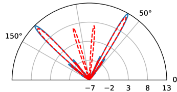
(a) $K=2$, $N=32$.

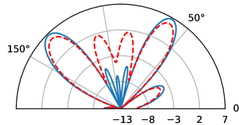
(b) $K=2$, $N=8$.

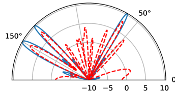
(c) $K=3$, $N=32$.

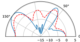
(d) $K=3$, $N=8$.

Figure 3: Array directivity [dB] of the useful signal (blue) and third-order distortion (dashed red). Equal power is sent to each user and $d=\lambda_{c}/2$. User angles $\theta$ are: 135°, 60° and 150°. As the number of users ($K$) increases, more intermodulation beams appear, the distortion becomes more uniformly distributed and the ratio of the array gain for the useful signal versus the distortion increases. Reducing the number of antennas ($N$) at the array induces a large beam width and thus a more uniform distribution.

III-B Comparison of central vs distributed for the single-user case

The performance of a central massive MIMO system can be retrieved by setting $M=1$. In that case, we can drop the index $m$ and (12) simplifies to

$${S}_{rr}(\omega)= \left(S_{\mathrm{sig}}(\omega)+S_{\mathrm{dis}}(\omega)\right)|\beta|^{2}|D_{N}(\phi^{(1)}-\phi)|^{2}.$$ (14)

Comparing (12) and (14), we can observe that in central massive MIMO, the spatial gain is determined by the angular direction of the given location $\phi$ with respect to the array, together with the path loss $|\beta|^{2}$, which is mainly distance dependent. In distributed massive MIMO, the spatial gain depends on more parameters, which makes it focused on a ’beamspot’ space: i) The path loss coefficient $\beta_{m}$ with respect to each array. ii) the directions $\phi_{m}$ with respect to each array. iii) The propagation delay $\tau_{m}$ with respect to each array. iv) The phase shift $\psi_{m}=2\pi f_{c}\tau_{m}$. The fact that the signal coming from each array will arrive with a different timing offset will induce a combining that is in general non-coherent at unintended locations. This effect can be seen as small scale fading since it varies with displacement on the order of the wavelength and is highly frequency dependent. This fading will become Rayleigh distributed as the number of arrays grows large and their contributions are similar. The particularity here is that the Rayleigh fading is not due to $M$ reflective components of a single transmit signal, since the channel is in pure LoS, yet originates from the non-coherent transmissions from $M$ arrays at the unintended locations. If the location is much closer to one specific array $m$, its contribution can be much stronger than the contributions of other arrays. In that case, the fading will look more like Rician fading.

Figure 4: Spatial focusing [dB] of the distortion for $K=2$ and $K=3$ users located at red crosses. Axis are in meters units. The distortion becomes more uniformly distributed going from the the single array ($M=1$) to the distributed case ($M=4$) together with an increasing number of users. Moreover, small-scale fading effects can be observed in the distributed case at locations where multiple beams are crossing.

III-C Multi-User Case

III-C1 Useful Signal Part

In the multi-user case, $K$ signals are beamformed in the direction of each UE from each array. The useful signal part of (3) is given by the term $l=1$. Using (7), it is given by

$$b_{1}x_{m,n}(t)=b_{1}\sum_{k=1}^{K}e^{\jmath\phi_{m}^{(k)}n+\jmath\psi_{m}^{(k)}}s^{(k)}(t+\tau_{m}^{(k)}),$$

where we see that each array beamforms in the $K$ directions of the users, i.e., $\phi_{m}^{(k)}$ for $k=1,...,K$. Using the same steps as in previous sections, the PSD of the useful signal part at the observer location can be computed as

$${S}_{\mathrm{sig}}(\omega)=c_{1}S(\omega)\sum_{k=1}^{K}p^{(k)}$$

$$\left|\sum_{m=1}^{M}|\beta_{m}|D_{N_{m}}(\phi_{m}^{(k)}-\phi_{m})e^{\jmath(\psi_{m}^{(k)}-\psi_{m})+\jmath\omega(\tau_{m}^{(k)}-\tau_{m})}\right|^{2}.$$

The radiation pattern of the signal radiated by one of the arrays is obtained as a particular case of this expression for the array in question, i.e., we set $M=1$ and we drop the array index $m$

$$P_{\mathrm{sig}}(\omega)=S(\omega)c_{1}|\beta|^{2}\sum_{k=1}^{K}p^{(k)}\left|D_{N_{m}}(\phi^{(k)}-\phi)\right|^{2}.$$

Using the relationship $\phi=\frac{2\pi}{\lambda_{c}}d\cos(\theta)$, Fig. 3 plots in blue the array directivity for the useful signal, i.e., normalized with respect to an isotropic radiator. Note that the directivity does not depend on the frequency $\omega$, the PA coefficient $c_{1}$ and $\beta$.

III-C2 Distortion Term

We now focus on the third-order distortion term, i.e., the term of the sum corresponding to $l=3$ in (3). Using (7), we find that

$$b_{3}x_{m,n}(t)|x_{m,n}(t)|^{2}=b_{3}\sum_{k=1}^{K}\sum_{k^{\prime}=1}^{K}\sum_{k^{\prime\prime}=1}^{K}e^{\jmath\phi_{m}^{(k,k^{\prime},k^{\prime\prime})}n}$$

$$e^{\jmath\psi^{(k,k^{\prime},k^{\prime\prime})}_{m}}s^{(k)}(t+\tau_{m}^{(k)})s^{(k^{\prime})}(t+\tau_{m}^{(k^{\prime})})(s^{(k^{\prime\prime})}(t+\tau_{m}^{(k^{\prime\prime})}))^{*},$$

where $\psi^{(k,k^{\prime},k^{\prime\prime})}_{m}=\psi_{m}^{(k)}+\psi_{m}^{(k^{\prime})}-\psi_{m}^{(k^{\prime\prime})}$ and $\phi_{m}^{(k,k^{\prime},k^{\prime\prime})}=\phi_{m}^{(k)}+\phi_{m}^{(k^{\prime})}-\phi_{m}^{(k^{\prime\prime})}$. As compared to the single-user case, the distortion is beamformed not only in the user directions but also several other intermodulation directions [7]. To clarify this, let us look at the received PSD. Using the same steps as in previous sections, the PSD of the third-order distortion at the observer location can be computed as

$${S}_{\mathrm{dis}}^{(1)}(\omega)= c_{3}\sum_{k,k^{\prime},k^{\prime\prime}}p^{(k)}p^{(k^{\prime})}p^{(k^{\prime\prime})}\sum_{m,m^{\prime}}|\beta_{m}||\beta_{m^{\prime}}|$$

$$e^{\jmath(\psi^{(k,k^{\prime},k^{\prime\prime})}_{m}-\psi^{(k,k^{\prime},k^{\prime\prime})}_{m^{\prime}})-\jmath\omega(\tau_{m}-\tau_{m^{\prime}})}S^{(3)}_{m,m^{\prime},k,k^{\prime}}(\omega)$$

$$D_{N_{m}}(\phi_{m}^{(k,k^{\prime},k^{\prime\prime})}-\phi_{m})(D_{N_{m^{\prime}}}(\phi_{m^{\prime}}^{(k,k^{\prime},k^{\prime\prime})}-\phi_{m^{\prime}}))^{*},$$

where $S^{(3)}_{m,m^{\prime},k,k^{\prime}}(\omega)=\frac{1}{4\pi^{2}}e^{\jmath\omega\Delta\tau_{m,m^{\prime}}^{(k)}}S(\omega)\circledast e^{\jmath\omega\Delta\tau_{m,m^{\prime}}^{(k^{\prime})}}S(\omega)\circledast e^{\jmath\omega\Delta\tau_{m,m^{\prime}}^{(k^{\prime\prime})}}S(-\omega)$, with $\Delta\tau_{m,m^{\prime}}^{(k)}=\tau_{m}^{(k)}-\tau_{m^{\prime}}^{(k)}$. The distortion radiation pattern of a specific array is obtained as a particular case of this expression for the array in question, i.e., we set $M=1$ and we drop the array index $m$

$$P_{\mathrm{dis}}^{(1)}(\omega)= S^{(3)}(\omega)c_{3}|\beta|^{2}\sum_{k,k^{\prime},k^{\prime\prime}}p^{(k,k^{\prime},k^{\prime\prime})}|D_{N}(\phi^{(k,k^{\prime},k^{\prime\prime})}-\phi)|^{2},$$

with $p^{(k,k^{\prime},k^{\prime\prime})}=p^{(k)}p^{(k^{\prime})}p^{(k^{\prime\prime})}$. Similarly as for the useful signal, we can define the array directivity of the third-order distortion as $P_{\mathrm{dis}}^{(1)}(\omega,\phi)$ normalized by a isotropically radiated distortion.It is shown in dashed red in Fig. 3, with related explanations, and in accordance with previous work [4].

The set of beam directions are given by the potential combinations of directions $\phi^{(k,k^{\prime},k^{\prime\prime})}=\phi^{(k)}+\phi^{(k^{\prime})}-\phi^{(k^{\prime\prime})}$, for $k,k^{\prime},k^{\prime\prime}=1,...K$. This results in a total of $K^{3}/2-K^{2}/2+K$ different directions. As an example, for $K=2$, a total of 4 directions are possible: $\phi^{(1)},\phi^{(2)},2\phi^{(2)}-\phi^{(1)},2\phi^{(1)}-\phi^{(2)}$. The power of each beam also depends on the allocated power $p^{(k)}$ to each UE. In some cases, directions can combine, resulting in a lower total number of beams. As $N$ decreases, the beam width increases and beam directions are more likely to overlap and to combine, resulting in a more uniform distribution (see Fig. 3 (c) and (d)). As a comparison with a central massive MIMO system ($M=1$), a distributed massive MIMO system with the same total number of antennas will induce a more uniformly spread distortion since: i) the array gain in main beam directions will be reduced and ii) the beam width will be wider and different beam directions are more likely to overlap. As a result, the distortion becomes uniformly distributed. These effects can be expected from Fig. 3 by considering a single $32$-antenna array versus four $8$-antenna arrays. Moreover, the distortion gets more uniformly beamformed with increasing number of distinct UEs directions.

IV Spatial Distribution in a Cell

In this section we study the spatial distribution of the signal and the third-order distortion, for a $100m\times 100m$ square cell, as shown in Fig. 4. We compare the performance of a $M=4\times N=8$ distributed system with a $M=1\times N=32$ central system. To study the radiated power at observer locations, we sample the cell with a spatial step of $\lambda_{c}/2$, which captures small scale fading effects. A path loss exponent of $2.5$ is used. The figure of merit under study is the spatial focusing, defined as the power radiated at a certain location versus an ideally uniformly distributed power radiation. In other words, ${S}_{\mathrm{sig}}(\omega)$ and ${S}_{\mathrm{dis}}^{(1)}(\omega)$ are respectively normalized by their average computed on the whole $100\text{\,}\mathrm{m}$$\times$$100\text{\,}\mathrm{m}$ cell area. The spatial focusing does not depend on the PA parameters ($c_{1}$ and $c_{3}$) and can be seen as a spatial generalization of the array directivity. The spatial focusing is evaluated at carrier frequency $f_{c}=1$ GHz, for a raised cosine PSDs $S(\omega)$. Fig. 4 clearly shows that the distortion becomes more uniformly distributed going from: i) the single array $M=1$ to the distributed case ($M=4$) and ii) $K=2$ to $K=3$ users. Moreover, one can notice in the distributed case the so-called small scale fading effect, previously described and resulting from the non-coherent combining of the transmissions from the $M$ arrays.

V Conclusion

We have shown in this paper that the distortion due to nonlinear PA is not always uniformly distributed in space. In the single-user LoS case, it coherently adds up at the user location. In the few users case, with a few distinct beam directions, the signals will add up at the user locations plus several others locations. As the number of beam directions increases, it quickly becomes close to uniformly distributed. As a comparison with a massive MIMO system having the same total number of antennas, the distortion in distributed massive MIMO is considerably more uniformly distributed in space. Moreover, the potential coherent combining is contained in a beamspot rather than in generic directions and it is subject to small-scale fading effects. As a general conclusion, we can expect that going distributed allows working significantly closer to saturation, directly improving the PA efficiency. Future works will target a quantitative assessment of this improvement.

References

- [1] H. Q. Ngo, A. Ashikhmin, H. Yang, E. G. Larsson, and T. L. Marzetta, “Cell-Free Massive MIMO Versus Small Cells,” IEEE Trans. Wireless Commun., vol. 16, no. 3, pp. 1834–1850, 2017.
- [2] E. Björnson, J. Hoydis, M. Kountouris, and M. Debbah, “Massive MIMO Systems With Non-Ideal Hardware: Energy Efficiency, Estimation, and Capacity Limits,” IEEE Trans. Inf. Theory, vol. 60, no. 11, pp. 7112–7139, 2014.
- [3] E. G. Larsson and L. Van der Perre, “Out-of-Band Radiation From Antenna Arrays Clarified,” IEEE Commun. Lett., vol. 7, no. 4, pp. 610–613, 2018.
- [4] C. Mollén, U. Gustavsson, T. Eriksson, and E. G. Larsson, “Spatial Characteristics of Distortion Radiated From Antenna Arrays With Transceiver Nonlinearities,” IEEE Trans. Wireless Commun., vol. 17, no. 10, pp. 6663–6679, 2018.
- [5] F. Horlin and A. Bourdoux, Digital Compensation for Analog Front-Ends. Wiley, 2008.
- [6] C. Mollén, “The Hermite-Polynomial Approach to the Analysis of Nonlinearities in Signal Processing Systems,” in High-End Performance with Low-End Hardware: Analysis of Massive MIMO Base Station Transceivers. Linköping University Electronic Press, 2017, p. 215.
- [7] C. Hemmi, “Pattern Characteristics of Harmonic and Intermodulation Products in Broadband Active Transmit Arrays,” IEEE Trans. Antennas Propag., vol. 50, no. 6, pp. 858–865, 2002.