Line-depth ratios as indicators of effective temperature and surface gravity

Abstract

The analysis of stellar spectra depends upon the effective temperature (${T_{\mathrm{eff}}}$) and the surface gravity ($\log g$). However, the estimation of $\log g$ with high accuracy is challenging. A classical approach is to search for $\log g$ that satisfies the ionization balance, i.e., the abundances from neutral and ionized metallic lines being in agreement. We propose a method of using empirical relations between ${T_{\mathrm{eff}}}$, $\log g$ and line-depth ratios, for which we meticulously select pairs of Fe i and Fe ii lines and pairs of Ca i and Ca ii lines. Based on $YJ$-band (0.97–1.32 $\mu$m) high-resolution spectra of 42 FGK stars (dwarfs to supergiants), we selected five Fe i–Fe ii and four Ca i–Ca ii line pairs together with 13 Fe i–Fe i pairs (for estimating ${T_{\mathrm{eff}}}$), and derived the empirical relations. Using such relations does not require complex numerical models and tools for estimating chemical abundances. The relations we present allows one to derive ${T_{\mathrm{eff}}}$ and $\log g$ with a precision of around 50 K and 0.2 dex, respectively, but the achievable accuracy depends on the accuracy of the calibrators’ stellar parameters. It is essential to revise the calibration by observing stars with accurate stellar parameters available, e.g., stars with asteroseismic $\log g$ and stars analyzed with complete stellar models taking into account the effects of non-local thermodynamic equilibrium and convection. In addition, the calibrators we used have a limited metallicity range, $-0.2<{\mathrm{[Fe/H]}}<+0.2$ dex, and our relations need to be tested and re-calibrated based on a calibrating dataset for a wider range of metallicity.

1 Introduction

Surface gravity, $\log g$, is a fundamental stellar parameter that depends on stellar mass and radius. In stellar astrophysics, the unit of $g$ is cm s^-2. The surface gravity of the Sun, $g_{\odot}=27\,400$ cm s^-2, corresponds to $\log g_{\odot}=4.44$ dex. From the spectroscopic point of view, surface gravity affects various kinds of absorption features, such as the damping wings of hydrogen lines. Several methods have been developed for estimating the value of $\log g$ on the basis of such features (see, e.g., Catanzaro, 2014). However, it is not easy to determine $\log g$ with a high accuracy, and many methods require complex calculations with numerical models. Systematic differences are often found between the spectroscopic $\log g$ estimates and those derived using other approaches (e.g., asteroseismic analysis; Morel & Miglio 2012; Chaplin & Miglio 2013; Mészáros et al. 2013; Mortier et al. 2014).

The main spectral features of stars with the middle spectral types (i.e., F, G and K types) are the metallic absorption lines that characterize their spectra. Among these lines, ionized lines are particularly sensitive to $\log g$. According to the Saha equation, the ratio of atoms to ions in the stellar atmosphere is proportional to the electronic pressure, $P_{e}$, when the local thermodynamic equilibrium (LTE) holds and only one ionization stage is available. Therefore, the ionization fraction is higher with a lower $\log g$, and thus, lower $P_{e}$ (Gray, 2005). Based on this behaviour, it is possible to estimate $\log g$ by postulating that the iron abundance derived from Fe ii lines ($\log g$-sensitive) and the counterpart with Fe i lines ($\log g$-insensitive) agree with each other. This method has been used quite often (Gray & Kaur, 2019; Tsantaki et al., 2019, and references therein), but some authors have questioned the simple assumption of the balance between Fe i and Fe ii lines under the LTE condition (Fuhrmann et al. 1997; Kovtyukh & Andrievsky 1999; Korn, Shi, & Gehren 2003). In addition, previous studies almost always relied on Fe ii lines in the optical spectra. Recently, Marfil et al. (2020) explored Fe ii lines in the infrared range together with those in the optical range and detected only two Fe ii lines that are available for estimating stellar parameters including $\log g$.

Another commonly-taken approach is to determine various stellar parameters including ${T_{\mathrm{eff}}}$, $\log g$ and the metallicity (or a bit more detailed chemical abundances) by searching for the synthetic spectrum that matches a given observed spectrum best. The selected synthetic spectrum is required to reproduce many absorption lines, in a wide spectral range, that have different sensitivity to the stellar parameters. A large set of synthetic spectra and an efficient tool for the optimization such as FERRE (García Pérez et al., 2016) need to be prepared, and such analysis has been regularly performed, especially for a large-scale spectroscopic survey (e.g. Allende Prieto et al., 2006, 2014; García Pérez et al., 2016). The resultant precision and accuracy depend on how well the selected synthetic spectrum reproduces the observed one. Synthetic spectra for the optical range are considered to be sufficiently good for stars in a wide range of stellar parameters, and this is also true for the spectral band of the APOGEE (a part of the $H$ band) thanks to their great effort to establish the line list (Shetrone et al., 2015). However, as mentioned above, thus-derived $\log g$ tend to show systematics compared to $\log g$ from other approaches. For other wavelength ranges in the infrared, the line information tends to have large errors currently (see, e.g., Andreasen et al., 2016). For example, Fukue et al. (2021) compiled a list of more than 250 lines of several elements seen in the $YJ$ band (0.97–1.32 $\mu$m), including the lines of Fe i reported in Kondo et al. (2019), that appear relatively isolated in K-type giants. Fukue et al. (2021) found that the scatter in the derived abundances are larger than the results for other wavelengths (see their Section 3.3), and there appears a systematic offset by 0.1–0.2 dex between the results with the oscillator strengths, $\log gf$, given in two line lists, the Vienna Atomic Line Database (VALD; Ryabchikova et al., 2015) and Meléndez & Barbuy (1999). Such errors and systematics limit the quality of synthetic spectra and thus the precision of the stellar parameters derived with the spectral synthesis.

In this study, we propose a new method for determining the surface gravity on the basis of neutral and ionized lines without being affected directly by the uncertainty in the line list. We focus on the Fe i, Fe ii, Ca i and Ca ii lines in the $YJ$ bands. Moreover, we consider line-depth ratios (LDRs) as indicators of both temperature and surface gravity with which the inference of chemical abundances is unnecessary. An advantage of LDRs is that their use is based on empirical relations, which do not require sophisticated calculations with numerical models. The accuracy of the $\log g$, derived from the LDR empirical relations, relies on the accuracy of the calibrators’ $\log g$, but it is trivial to revise the calibration when the new data set for better calibrators becomes available.

LDRs have been often used for estimating ${T_{\mathrm{eff}}}$. LDRs of lines with different excitation potentials (EPs) are sensitive to ${T_{\mathrm{eff}}}$, and thus, most previous works explored the use of LDRs as temperature indicators (Gray & Johanson, 1991; Fukue et al., 2015, and references therein). However, LDRs of some kinds of line pairs depend not only on ${T_{\mathrm{eff}}}$ but also on $\log g$ and other stellar parameters. Jian et al. (2020) compared the LDRs of dwarfs, giants and supergiants, and found that LDRs of some line pairs at each ${T_{\mathrm{eff}}}$ depend on $\log g$. They examined the line pairs of neutral atoms, e.g., Ca i–Si i, and concluded that the differences in ionization potentials of the atoms can explain the different dependencies of line depth on $\log g$. LDRs also depend on metallicity and abundance ratios (see, e.g., Jian, Matsunaga, & Fukue, 2019, on the metallicity effect), and these effects would complicate the determination of $\log g$ together with ${T_{\mathrm{eff}}}$. This uncertainty may be avoided if we combine lines of the same element (Taniguchi et al., 2021). Therefore, we consider line pairs of the same element only. We use Fe i–Fe i pairs for determining ${T_{\mathrm{eff}}}$, and Fe i–Fe ii and Ca i–Ca ii pairs for determining $\log g$.

The main goal of this paper is two fold: (1) to demonstrate that empirically-calibrated LDR relations can be used for estimating $\log g$ of stars over a wide range of luminosity class and (2) to identify the useful line pairs available in the $YJ$ bands. We use 42 $YJ$-band spectra of FGK stars, dwarfs to supergiants, adopted from Jian et al. (2020). Their sample was not collected for allowing us the calibration based on the most accurate surface gravities, and the lack of “benchmark stars” with high-resolution $YJ$-band spectra limits the accuracy of the LDR relations we can derive in this study. Nevertheless, we can show that the LDR relations give useful constraints to $\log g$ together with ${T_{\mathrm{eff}}}$. The $YJ$ bands, in particular the $Y$ band, are uniquely important in determining the surface gravities of reddened stars because these bands are less affected by interstellar extinction ($A_{Y}/A_{V}\sim 0.4,~{}A_{J}/A_{V}\sim 0.3$) and host more ionized lines than other near-infrared bands (Andreasen et al., 2016; Marfil et al., 2020). Many high-resolution spectrographs covering $YJ$ have been in operation: e.g., GIANO (Caffau et al., 2019), HPF (Sneden et al., 2021), IRD (Kotani et al., 2018) and CRIRES+ (Follert et al., 2014) in addition to WINERED with which our data were collected.

2 Data

We make use of spectra of 42 objects with ${T_{\mathrm{eff}}}$ between 4800 K and 6300 K (Table 1) adopted from Jian et al. (2020). The WINERED spectrograph was used to collect the $YJ$-band spectra with a resolution of around 28 000 (see the instrumental details on the WINERED in Ikeda et al., 2016). The observations were carried out with the 1.3 m Araki Telescope at Koyama Observatory, Kyoto Sangyo University in Japan from October 2015 to May 2016. The reduction in the spectroscopic data was described in Jian et al. (2020) and Matsunaga et al. (2020). The initial steps of the reduction were performed using the WINERED pipeline (Hamano et al. in preparation). Then, the telluric absorption lines were removed using the observed spectra of telluric standard stars with the method developed in Sameshima et al. (2018), except for the 53rd–54th orders (10280–10680 Å) in which significant telluric lines were rather scarce. The continuum level in every spectrum was normalized to the unity. In addition to the reduced spectra, the pipeline gives estimates of the signal-to-noise ratios (S/N) for three parts of each order by comparing spectra of multiple exposures with each other. We use these S/N values for evaluating the errors of line depths, discussed below. Fig. 1 presents the effective S/N for which the S/N values of objects and those of telluric standards are combined except the 53rd–54th orders (see also Section 3.2).

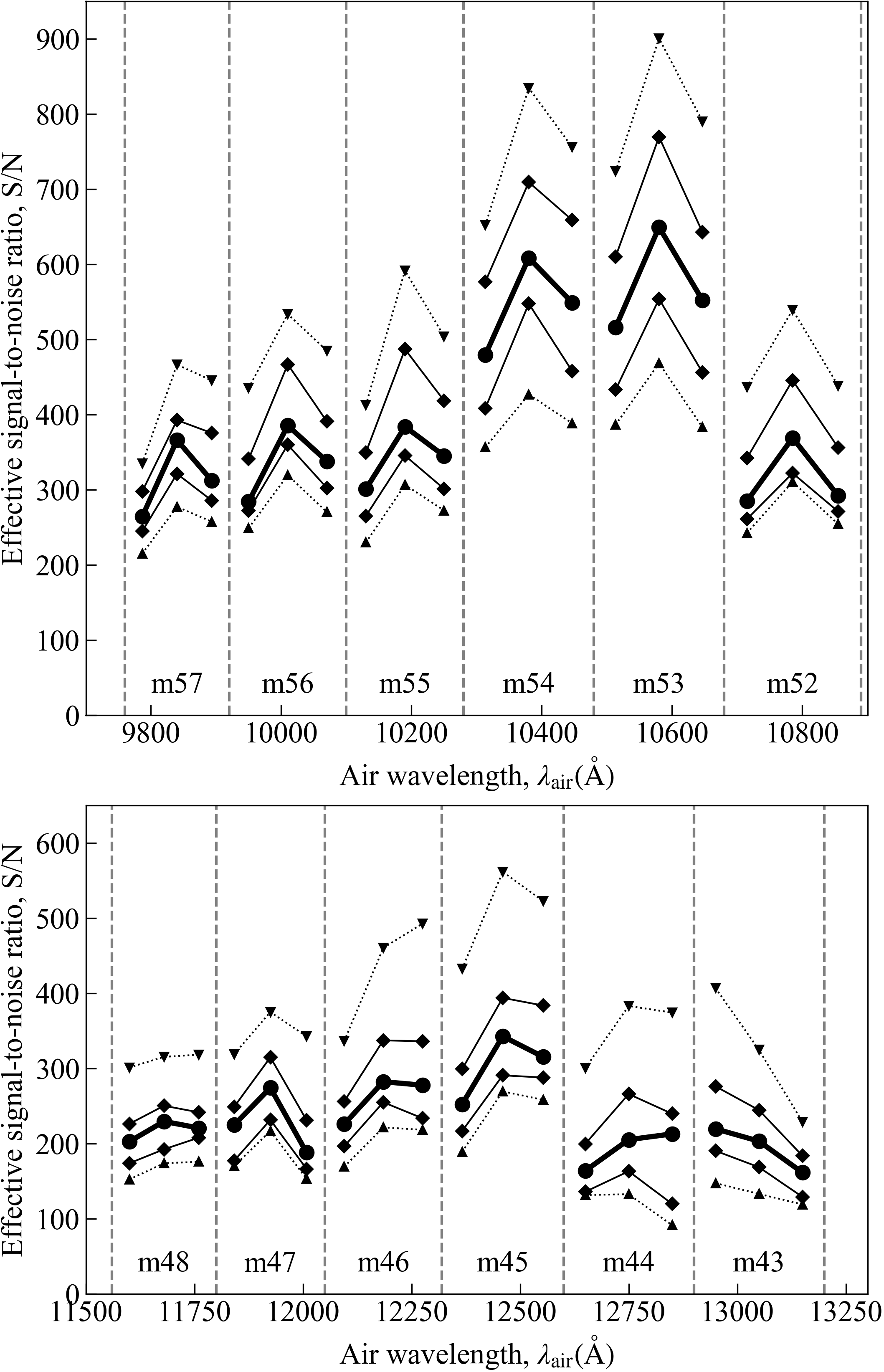
Figure 1: Effective signal-to-noise ratios at three parts of each order (52nd to 57th in $Y$, upper panel, and 43rd to 48th in $J$, lower panel). The S/N values measured by the WINERED pipeline for each target and the corresponding telluric standard are combined to give the effective S/N, except the 53rd and 54th order for which the S/N for the target is used. The S/N values for the spectra of the 42 targets (Table 1) are considered here, and the five points at each wavelength indicate 10, 25, 50, 75 and 90 percentiles, from top to bottom, corresponding to the 4th, 10th, 21st, 31st and 37th values.

Our sample is composed of late F to early K-type stars, and the surface gravity ranges from 1.35 to 4.5 dex. The distribution on the $(\log g,~{}{T_{\mathrm{eff}}})$ plane is, however, not homogeneous (Fig. 2). Jian et al. (2020) selected these objects, together with stars in a broader ${T_{\mathrm{eff}}}$ range, because the optical LDRs were investigated by Kovtyukh et al. (2003, 2006) and Kovtyukh (2007). In the following analysis, we use the stellar parameters that Jian et al. (2020) compiled from a few studies (Kovtyukh, Soubiran, & Belik, 2004; Prugniel, Vauglin, & Koleva, 2011; Park et al., 2013; Liu et al., 2014; Luck, 2014; da Silva, Milone, & Rocha-Pinto, 2015). Although the measurements in these studies were all based on spectroscopic data, the compiled $\log g$ values are not homogeneous because of multiple differences, such as those in the spectral resolution and in the absorption features that had major impacts on the estimates. The selection of the objects in Jian et al. (2020) was not done for securing the homogeneous $\log g$ values. However, it is difficult to find a set of $YJ$-band high-resolution spectra of stars, extending from dwarfs to supergiants, with homogeneous and accurate $\log g$ available. In Section 4.2, we consider a subset of our objects with $\log g$ taken from different studies to discuss the accuracy of the gravity scale.

Table 1: The objects used for deriving the LDR relations listed in descending order of ${T_{\mathrm{eff}}}$. The stellar parameters are adopted from Jian et al. (2020), and the last column indicates the table in the paper in which each star was listed.

Object	${T_{\mathrm{eff}}}$	$\log g$	${\mathrm{[Fe/H]}}$	Obs. date	Table
	(K)	(dex)	(dex)
HD 194093	6202	1.35	$0.05$	2015.10.26	Table 3
HD 171635	6201	1.78	$-0.10$	2016.03.11	Table 3
HD 102870	6055	4.00	$0.18$	2016.01.27	Table 1
HD 137107	6037	4.30	$0.05$	2016.01.26	Table 1
HD 115383	6012	4.30	$0.16$	2016.01.26	Table 1
HD 19373	5963	4.20	$0.11$	2016.03.11	Table 1
HD 39587	5955	4.30	$0.02$	2016.03.17	Table 1
HD 114710	5954	4.30	$0.12$	2016.01.26	Table 1
HD 34411	5890	4.20	$0.15$	2016.02.28	Table 1
HD 95128	5887	4.30	$0.06$	2016.02.03	Table 1
HD 141004	5884	4.10	$0.03$	2016.02.27	Table 1
HD 72905	5884	4.40	$-0.02$	2016.01.27	Table 1
HD 143761	5865	4.30	$-0.06$	2016.01.26	Table 1
HD 117176	5611	3.86	$-0.10$	2016.01.26	Table 1
HD 101501	5558	4.50	$0.02$	2016.01.26	Table 1
HD 204867	5466	1.54	$0.03$	2015.10.26	Table 3
HD 31910	5441	1.57	$-0.01$	2015.10.31	Table 3
HD 92125	5354	2.22	$0.03$	2016.03.21	Table 3
HD 26630	5337	1.74	$0.09$	2015.10.28	Table 3
HD 3421	5302	1.88	$-0.20$	2015.10.31	Table 3
HD 74395	5264	1.41	$0.09$	2016.01.27	Table 3
HD 10476	5242	4.30	$0.00$	2015.10.31	Table 1
HD 159181	5220	1.50	$-0.15$	2016.02.03	Table 3
HD 68312	5090	2.70	$-0.12$	2016.03.15	Table 2
HD 78235	5070	3.00	$-0.03$	2015.10.28	Table 2
HD 76813	5060	2.63	$-0.06$	2015.10.28	Table 2
HD 62345	5032	2.61	$-0.01$	2016.01.27	Table 2
HD 34559	5010	2.74	$0.00$	2016.01.19	Table 2
HD 27348	5003	2.75	$0.05$	2015.10.25	Table 2
HD 11559	4977	3.23	$0.16$	2015.10.23	Table 2
HD 202109	4976	1.90	$0.10$	2016.03.21	Table 3
HD 27697	4975	2.64	$0.12$	2015.10.25	Table 2
HD 27371	4960	2.76	$0.15$	2015.10.28	Table 2
HD 77912	4957	1.75	$-0.14$	2016.03.21	Table 3
HD 99648	4942	2.24	$-0.03$	2016.03.12	Table 3
HD 122064	4937	4.50	$0.12$	2016.02.03	Table 1
HD 28305	4925	2.72	$0.20$	2015.10.25	Table 2
HD 219134	4900	4.20	$0.10$	2015.10.25	Table 1
HD 198149	4858	3.29	$-0.19$	2015.10.26	Table 2
HD 19787	4832	2.92	$0.12$	2016.03.11	Table 2
HD 82106	4827	4.10	$-0.06$	2016.03.12	Table 1
HD 79555	4803	4.10	$-0.14$	2016.05.01	Table 1

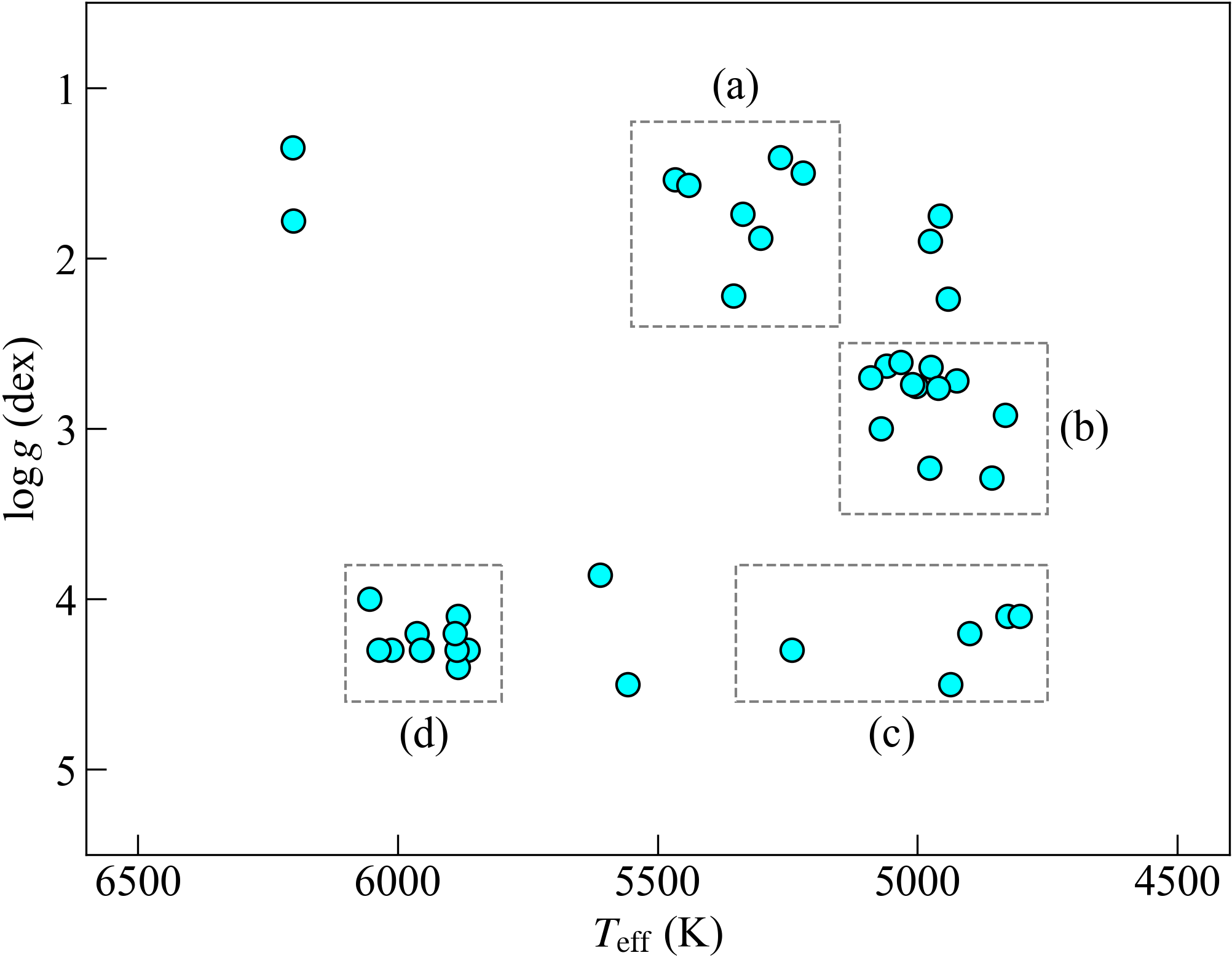
Figure 2: Distribution of the objects (Table 1) on the $({T_{\mathrm{eff}}},~{}\log g)$ plane. The groups, (a)–(d), are used for selecting line pairs that are useful over a wide range of this plane in Section 3.4.

HD 137107 ($\eta$ CrB A, with ${T_{\mathrm{eff}}}=6037$ K and $\log g=4.30$ dex) is a double-lined spectroscopic binary (Pourbaix, 2000). The lines of the two components are not split from each other in our spectrum (see, also, Duquennoy, Mayor, & Halbwachs, 1991), but the lines look slightly broader than those in other objects (Section 3.2). Because the two components of this binary system are similar to each other, both being early G-type dwarfs with ${\sim}1.2\,{M_{\odot}}$ (Muterspaugh et al., 2010), we include this object in our analysis. There are six spectroscopic binaries among our sample, according to Pourbaix et al. (2004), and HD 137107 is the only double-lined system among them.

3 Analysis

3.1 Line selection based on synthetic spectra

To perform the line selection, we searched for the lines of the four elements (Fe i, Fe ii, Ca i and Ca ii) that may be included in line pairs showing tight LDR relations. We consider the lines within 9760–10890 and 11600–13200 Å, corresponding to the echelle orders of 52–57th ($Y$ band) and 43–48th ($J$ band) of WINERED. Not many elements show both neutral and ionized lines. Other than Fe and Ca, some elements such as Si and Ti show one or more lines of the neutral and ionized states together for each element. Looking at the spectra for the lines of those elements, however, we decided not to include them in our analysis because it would be impossible to construct multiple pairs of lines that demonstrate useful LDR relations for our purpose. We focus on Fe and Ca in this study, although other elements may be useful for different ${T_{\mathrm{eff}}}$ ranges.

For each of the atoms and ions, we selected the candidates of lines to use on the basis of the synthetic spectra created with MOOG (the version released in 2017 February, Sneden et al., 2012). We used the VALD and the 1D plane-parallel atmosphere models compiled by R. Kurucz  for synthesizing the following three kinds of spectra:

(i)

the spectra with all the atomic and molecular lines included,

(ii)

the spectra with only one of the four species (Fe i, Fe ii, Ca i and Ca ii) included,

(iii)

the spectra with all the atomic and molecular lines included except one of the four species.

The spectra were synthesized for a grid of $({T_{\mathrm{eff}}},~{}\log g)$ covering the range of Fig. 2. For each wavelength, the three kinds of synthetic spectra give three theoretical depths—(i) $d_{\rm all}$, (ii) $d_{\rm one}$ and (iii) $d_{\rm out}$. We then listed up the line candidates that were expected to appear deep enough ($d_{\rm one}\gtrsim 0.03$) without heavy blends ($d_{\rm out}/d_{\rm all}\lesssim 0.2$) in a reasonably wide range on the $({T_{\mathrm{eff}}},~{}\log g)$ diagram. The numbers of the line candidates selected at this stage are 78 for Fe i, 7 for Fe ii, 12 for Ca i and 5 for Ca ii, giving 102 lines in total.

3.2 Depth measurements

For the expected wavelength $\lambda_{c}$ of each candidate line, we measured the depth in every observed spectrum by fitting a parabola, $f=a+b\lambda+c\lambda^{2}$, to four or five pixels around $\lambda_{c}$. We then obtained the position of the minimum ($\lambda_{0}$), the depth ($d$; the distance at $\lambda_{0}$ from the unity, i.e., $1-f(\lambda_{0})$), and the full-width at half-maximum (FWHM). If the parabola was not found to be convex downward, we rejected the fitting and ignored its measurement for the subsequent analysis. In addition, to take the error of each line depth into account, we considered the S/N values, which the WINERED pipeline gave for three parts of each order (Fig. 1). The S/N at $\lambda_{c}$ was estimated by interpolating the S/N values for the two consecutive parts around $\lambda_{c}$. The errors, indicated by the reciprocal of the S/N, of the spectra of an object and the telluric standard were combined in the quadrature to give the depth error, $e=\sqrt{e_{\rm obj}^{2}+e_{\rm tel}^{2}}$, except the 53rd and 54th orders for which $e=e_{\rm obj}$ because we did not make the telluric correction.

For each object, we measured the depths and the accompanying values for 102 or fewer lines that were not rejected. Then, we judged whether the measured absorptions were disturbed or not by examining the depths, wavelengths and widths that we obtained for each object. Suppose that we have $N_{\rm line}$ accepted measurements, i.e., the measured depth $d_{j}$, the depth error ($e_{j}$), the offset in wavelength ($V_{j}=c(\lambda_{0}-\lambda_{c})/\lambda_{c}$) and the FWHM ($W_{j}$) where $j$ varies from 1 to $N_{\rm line}$ for different lines. The wavelength offsets ($V_{j}$) and the FWHMs ($W_{j}$) are given in the velocity scale (${\rm km\,s^{-1}}$). Some measurements have to be discarded due to some reasons; e.g., weak lines may be under the detection limit, or there may be strong contaminating lines that disturb the target lines. We require the depth of each line to be more than 0.01, and then we can use the sufficiently deep lines to calculate the quartiles of the wavelength offset ($V_{1/4},~{}V_{2/4},~{}V_{3/4}$) and those of FWHM ($W_{1/4},~{}W_{2/4},~{}W_{3/4}$). The quartiles were used to detect outliers according to the interquartile range (IQR) rule, where the IQRs were given by ${\rm IQR}(V)=V_{3/4}-V_{1/4}$ and ${\rm IQR}(W)=W_{3/4}-W_{1/4}$. Every accepted measurement should account for the wavelength offset $V_{j}$ within $[V_{1/4}-3\,{\rm IQR}(V):V_{3/4}+3\,{\rm IQR}(V)]$ and the FWHM $W_{j}$ within $[W_{1/4}-3\,{\rm IQR}(W):W_{3/4}+3\,{\rm IQR}(W)]$. The acceptable range of $V$ was replaced with $[V_{2/4}-5:V_{2/4}+5]$ if ${\rm IQR}(V)$ is larger than $5\,{\rm km\,s^{-1}}$, while the range of $W$ was replaced with $[W_{2/4}-10:W_{2/4}+10]$ if ${\rm IQR}(W)$ is larger than $10\,{\rm km\,s^{-1}}$. In addition, the fractional errors of depth, $e_{j}/d_{j}$, needs to be smaller than 0.5. We performed the validation of measurements based on these conditions for every object. The FWHM, $W$, ranges from 15 to 23.5 ${\rm km\,s^{-1}}$ in the chosen 42 objects. HD 137107, the double-lined spectroscopic binary (Section 2), has the largest width, but the difference from the other objects is not very high (e.g., four others have $W$ larger than $20\,{\rm km\,s^{-1}}$).

3.3 Line selection based on observed spectra

In Section 3.2, we measured the depths of the lines selected by using synthetic spectra (Section 3.1), and validated the measurements. The next step is to select the lines that give depths validated for a significant fraction of objects over a wide range in the $({T_{\mathrm{eff}}},~{}\log g)$ plane. The selection of each line was made by considering the number and the ranges of ${T_{\mathrm{eff}}}$ and $\log g$ of the objects for which the measurements of the line were validated:

(i)

the number of the validated measurements should be 20 or more for each neutral line and 12 or more for each ionized line (among the 42 objects in total),

(ii)

the ${T_{\mathrm{eff}}}$ range should be 1000 K or wider,

(iii)

the $\log g$ range should be 2.5 dex or wider.

Table 2 lists the 97 lines confirmed (76 Fe i, 5 Fe ii, 11 Ca i and 5 Ca ii lines). Among these lines, Ca ii 9890.6280 includes two transitions with the oscillator strengths of $\log{gf}=0.900$ and $1.013$ at the same EP listed in VALD. The electric table provided in Supporting Information lists the combined strength ($\log{gf}=1.261$) with the “*” mark.

Table 2: List of the 97 confirmed lines that are used to search line-depth ratio pairs (see Section 3.3). The last column lists the number of objects for which the depth measurements were validated. Fe i, Fe ii, Ca i and Ca ii lines are combined together. The first 10 lines are presented here, and the full table is available in the supporting information section.

Species	$\lambda_{\mathrm{air}}$	EP	$\log{gf}$ (dex)		$N_{\mathrm{obj}}$
	(Å)	(eV)	VALD	MB99
Fe i	9800.3075	5.086	$-0.453$	—	37
Fe i	9811.5041	5.012	$-1.362$	—	41
Fe i	9861.7337	5.064	$-0.142$	—	42
Fe i	9868.1857	5.086	$-0.979$	—	42
Fe i	9889.0351	5.033	$-0.446$	—	41
Fe i	9944.2065	5.012	$-1.338$	—	40
Fe i	9980.4629	5.033	$-1.379$	—	42
Fe i	10041.472	5.012	$-1.772$	$-1.84$	37
Fe i	10065.045	4.835	$-0.289$	$-0.57$	40
Fe i	10081.393	2.424	$-4.537$	$-4.53$	33

3.4 LDR relations of individual line pairs

Using the lines in Table 2, we searched for line pairs that show tight LDR relations. The two lines in each line pair should be located in the same band, i.e. $Y$ (9760–10890 Å) or $J$ (11600–13200 Å). We ensured that a $Y$-band line was not combined with any $J$-band line. In the following analysis, we consider the LDR $r=d_{1}/d_{2}$, and its logarithm to the base 10, $\log r=\log(d_{1}/d_{2})$, where $d_{1}$ and $d_{2}$ indicate the depths of two lines. The following approximation formulae were used to obtain the errors in LDR ($y=r$ or $y=\log r$) on the basis of the errors in depth ($e_{1}$ and $e_{2}$, see Section 3.2).

$$e_{y}=\left\{\begin{array}[]{ll}\left(\frac{d_{1}}{d_{2}}\right)\sqrt{\left(\frac{e_{1}}{d_{1}}\right)^{2}+\left(\frac{e_{2}}{d_{2}}\right)^{2}}&~{}({\rm if}~{}y=r)\\ \left(\frac{1}{\ln 10}\right)\sqrt{\left(\frac{e_{1}}{d_{1}}\right)^{2}+\left(\frac{e_{2}}{d_{2}}\right)^{2}}&~{}({\rm if}~{}y=\log r)\end{array}\right.$$ (1)

3.4.1 Fe i–Fe i pairs

We use Fe i–Fe i pairs for determining ${T_{\mathrm{eff}}}$. The temperature dependency of line depth is characterized by the EP, and thus a pair of low-EP and high-EP lines is expected to be sensitive to ${T_{\mathrm{eff}}}$. For Fe i–Fe i pairs, every LDR is a ratio of the depth of a low-EP line to that of a high-EP line, $r=d_{\rm low}/d_{\rm high}$. For all the pairs of two lines whose EPs differ by 1 eV or more, we fitted the LDR–${T_{\mathrm{eff}}}$ relations with four different forms:

(T1)

$r=\alpha+\beta\,{T_{\mathrm{eff}}}$,

(T2)

$r=\alpha+\beta\,\log{T_{\mathrm{eff}}}$,

(T3)

$\log r=\alpha+\beta\,{T_{\mathrm{eff}}}$,

(T4)

$\log r=\alpha+\beta\,\log{T_{\mathrm{eff}}}$.

We made the least-square fitting with the weights $w=1/e_{y}^{2}$ given to each point, where $y$ is $r$ or $\log r$. If the two line depths of a given pair were accepted in all the objects, we would have 42 points to fit, but this is not the case in most line pairs. We ignored the line pairs for which the number of validated measurements, $N$, were smaller than 20 for the subsequent analysis. We also rejected relations with $\beta\geq 0$ because the depth ratio of a low-EP line to a high-EP line is expected to increase with decreasing ${T_{\mathrm{eff}}}$ in our target range. The weighted residual around each relation, $y=f(x)$, is given by

$$\sigma_{y}=\sqrt{\left.\sum_{i=1}^{N}w_{i}\left[y_{i}-f(x_{i})\right]^{2}\right/\sum_{i=1}^{N}w_{i}},$$ (2)

where $x$ stands for ${T_{\mathrm{eff}}}$ or $\log{T_{\mathrm{eff}}}$ according to the form among the four mentioned above. This $\sigma_{y}$ is converted to the scatter in ${T_{\mathrm{eff}}}$ around the fitted relation by

$$\sigma_{{T_{\mathrm{eff}}}}=\left\{\begin{array}[]{ll}\left|\sigma_{y}/\beta\right|&~{}({\rm if}~{}x={T_{\mathrm{eff}}})\\ (\ln 10)\,5400\,\left|\sigma_{y}/\beta\right|&~{}({\rm if}~{}x=\log{T_{\mathrm{eff}}})\end{array}\right..$$ (3)

We then rejected relations with $\sigma_{{T_{\mathrm{eff}}}}$ larger than 200 K.

In addition, in order to ensure that each relation can predict the LDRs of stars over a wide $({T_{\mathrm{eff}}},\log g)$ range of our targets suitably, we consider four groups of stars,

(a)

$5150<{T_{\mathrm{eff}}}<5550$ and $1.2<\log g<2.4$ (7 supergiants),

(b)

$4750<{T_{\mathrm{eff}}}<5150$ and $2.5<\log g<3.5$ (12 giants),

(c)

$4750<{T_{\mathrm{eff}}}<5350$ and $3.8<\log g<4.6$ (5 cool dwarfs),

(d)

$5800<{T_{\mathrm{eff}}}<6100$ and $3.8<\log g<4.6$ (11 warm dwarfs),

which are illustrated in Fig. 2. First, we rejected the line pairs for which the number of validated measurements for each group, $N_{\rm grp}$, were smaller than 3. Then, we compared the LDR-based temperatures ($T_{i}$ from $x_{i}=(y_{i}-\alpha)/\beta$) with the catalogue values ($T_{\mathrm{cat},\,i}$) and calculated the weighted mean of the deviation for each group,

$$D_{\rm grp}=\left.\sum_{i=1}^{N_{\rm grp}}w_{i}\left(T_{i}-T_{\mathrm{cat},\,i}\right)\right/\sum_{i=1}^{N_{\rm grp}}w_{i},$$ (4)

where the weight is given to each object according to the measurement error ($w_{i}=1/e_{y}^{2}$). If any of the $D_{\rm grp}$ values is larger than 120 K or smaller than $-120$ K, we rejected the given relation. Among the forms that were not rejected due to the conditions of $N_{\rm grp}$ and $D_{\rm grp}$, we selected the ones with the smallest $\sigma_{{T_{\mathrm{eff}}}}$ values for each line pair. We found 77 Fe i–Fe i accepted line pairs, where each absorption line may be used in many pairs. The relation between LDR ($r$ or $\log r$) and effective temperature (${T_{\mathrm{eff}}}$ or $\log{T_{\mathrm{eff}}}$) is illustrated in Fig. 3 for every line pair that we finally select (Section 3.5).

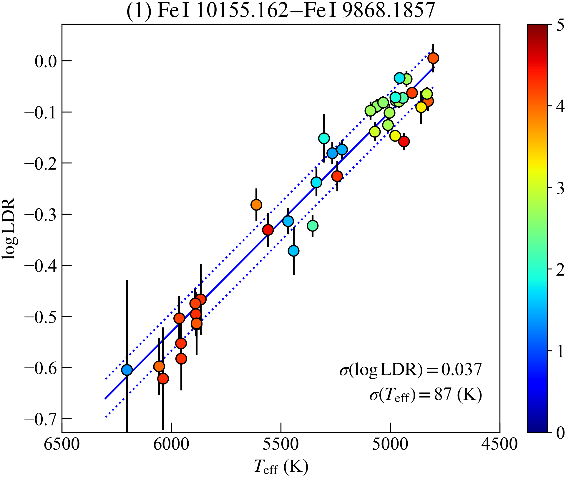
Figure 3: Relations between LDR ($r$ or $\log r$) and effective temperature (${T_{\mathrm{eff}}}$ or $\log{T_{\mathrm{eff}}}$). The points’ colours indicate $\log g$ according to the colour scale given on the right. The solid line indicates the LDR relation (Table 3) and the dotted lines indicate the width of $\pm\sigma_{y}$. Plots of all the 13 Fe i–Fe i pairs in Table 3 are given in Supporting Information.

3.4.2 Fe i–Fe ii and Ca i–Ca ii pairs

We use Fe i–Fe ii and Ca i–Ca ii pairs for determining $\log g$. For these pairs, every LDR is a ratio of the depth of a neutral line to that of an ionized line, i.e., $r=d_{\text{Fe\,{i}}}/d_{\text{Fe\,{ii}}}$ or $d_{\text{Ca\,{i}}}/d_{\text{Ca\,{ii}}}$. We searched for the LDR relations in the following forms:

(TG1)

$r=\alpha+\beta\,{T_{\mathrm{eff}}}+\gamma\,\log g$,

(TG2)

$r=\alpha+\beta\,\log{T_{\mathrm{eff}}}+\gamma\,\log g$,

(TG3)

$\log r=\alpha+\beta\,{T_{\mathrm{eff}}}+\gamma\,\log g$,

(TG4)

$\log r=\alpha+\beta\,\log{T_{\mathrm{eff}}}+\gamma\,\log g$.

We made the least-square fitting again with the weights $w=1/e_{y}^{2}$. The subsequent steps for selecting the line pairs and the forms of the LDR relations are similar to those for Fe i–Fe i pairs (Section 3.4.1), but the conditions are slightly different.

The minimum number of validated measurements required for each line pair is 12, instead of 20, considering that objects showing significant absorption in both neutral and ionized lines tend to be limited. The weighted residual around each relation, $y=f(x,\log g)$, is given by

$$\sigma_{y}=\sqrt{\left.\sum_{i=1}^{N}w_{i}\left[y_{i}-f(x_{i},~{}\log g_{i})\right]^{2}\right/\sum_{i=1}^{N}w_{i}},$$ (5)

where $x$ and $y$ stand for the temperature (${T_{\mathrm{eff}}}$ or $\log{T_{\mathrm{eff}}}$) and the LDR ($r$ or $\log r$), respectively. This $\sigma_{y}$ is converted to the scatter in $\log g$ around the fitting by

$$\sigma_{\log g}=\left|\sigma_{y}/\gamma\right|,$$ (6)

in addition to $\sigma_{T_{\mathrm{eff}}}$ given by equation (3), and we rejected relations with $\sigma_{\log g}$ larger than 0.5 dex.

We also considered the groups of objects in different parts of the $({T_{\mathrm{eff}}},\log g)$ plane, and calculated the weighted mean of the deviation in $\log g$,

$$D_{\rm grp}=\left.\sum_{i=1}^{N_{\rm grp}}w_{i}\left(\log g_{i}-\log g_{\mathrm{cat},i}\right)\right/\sum_{i=1}^{N_{\rm grp}}w_{i},$$ (7)

where $\log g_{i}$ equals $(y_{i}-\alpha-\beta x_{i})/\gamma$ in which $x_{i}$ is provided by the literature ${T_{\mathrm{eff}}}$, not the LDR-based one. We stipulated that $N_{\rm grp}$ be 3 or larger and $D_{\rm grp}$ be smaller than 0.5 dex for the groups (a) and (d), i.e. supergiants and warm dwarfs, but we did not consider the groups (b) and (c). Many of the Fe i–Fe ii and Ca i–Ca ii pairs lack validated measurements for the latter two groups because the ionized lines become too weak.

Finally, we found 175 Fe i–Fe ii pairs and 7 Ca i–Ca ii pairs. The relations between LDR ($r$ or $\log r$) and effective temperature (${T_{\mathrm{eff}}}$ or $\log{T_{\mathrm{eff}}}$) are illustrated in Fig. 4 for the line pairs that we finally select (Section 3.5). There are only 5 Fe ii lines (all the 5 in $Y$), but each of them is combined with many Fe i lines giving a large number of accepted pairs. The two lines used in Marfil et al. (2020), Fe ii 9997.598 and Fe ii 10501.500, are included. In contrast, both Ca i and Ca ii lines are limited in number (4 in $Y$ and 7 in $J$ of Ca i, and 3 in $Y$ and 2 in $J$ of Ca ii). While all the Fe ii lines are included in the line pairs accepted, any pair with Ca ii 9890.6280 was not accepted and only four Ca ii lines are included.

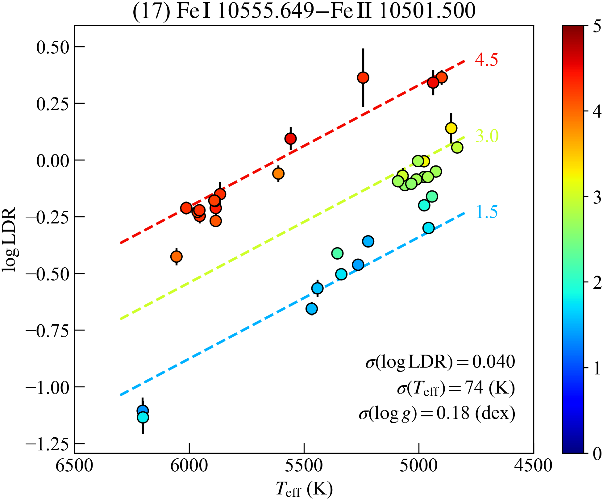
Figure 4: Relations between LDR ($r$ or $\log r$), effective temperature (${T_{\mathrm{eff}}}$ or $\log{T_{\mathrm{eff}}}$) and the surface gravity ($\log g$). The points’ colours indicate $\log g$ according to the colour scale given on the right. The three dashed lines indicate the LDR relations at $\log g=1.5$, 3.0 and 4.5 dex. Plots of all the 5 Fe i–Fe ii and 4 Ca i–Ca ii pairs in Table 3 are given in Supporting Information.

3.5 Selection of unique line pairs

The next step is to select a set of unique line pairs for which each line is not included in more than one pairs. The selection was made using a method similar to the one used by Taniguchi et al. (2018) but with different algorithms and formulae.

First, we give the scores of individual Fe i–Fe i line pairs,

$$E_{j}=\sqrt{\left(\sigma_{{T_{\mathrm{eff}}},j}\right)^{2}+e^{2}\,\left(\Delta\lambda_{j}\right)^{2}},$$ (8)

where $j$ stands for the temporary pair ID. Whereas $\sigma_{{T_{\mathrm{eff}}},j}$ is the residual around each relation (equation 3), $\Delta\lambda_{j}$ is the wavelength separation of the paired lines. Pairs with smaller $E_{j}$ values are preferred. The second term within the square root works as a penalty term that prevents the selection of pairs of lines with unnecessarily large wavelength separations, and we used the coefficient $e=0.2$ K Å^-1. Then, the score of a set of line pairs is given by

$$E=\frac{1}{{N_{\mathrm{pair}}}}\sqrt{\sum_{j=1}^{{N_{\mathrm{pair}}}}E_{j}^{2}}=\frac{1}{N_{\rm pair}}\sqrt{\sum_{j=1}^{N_{\rm pair}}\left(\sigma_{{T_{\mathrm{eff}}},j}\right)^{2}+e^{2}\,\sum_{j=1}^{N_{\rm pair}}\left(\Delta\lambda_{j}\right)^{2}},$$ (9)

where $N_{\rm pair}$ is the number of line pairs included in the set. In the case of the Fe i–Fe ii and Ca i–Ca ii pairs, we replace $\sigma_{{T_{\mathrm{eff}}}}$ in equations (8) and (9) with $\sigma_{\log g}$ and use a different coefficient $e$, $5\times 10^{-4}$ dex Å^-1.

Our purpose is to construct a set of line pairs whose $E$ is as small as possible. On the other hand, having many line pairs is advantageous. Adding an extra line pair is considered to be useful, even if it increases $E$ a little. We calculate the weighted means to estimate ${T_{\mathrm{LDR}}}$ and $\log\,{g_{\mathrm{LDR}}}$, preventing the final precision from degrading because of the extra pair. We have already selected line pairs with relatively small residuals (Section 3.4). Therefore, we try to find the set with the largest number of line pairs that has the smallest $E$ among the sets with the same number of line pairs.

It is simple to find such a set for the Fe i–Fe ii pairs. There are five Fe ii lines. For each of them, the pair given in Table 3 has the smallest $E_{1}$. We selected these five pairs, leading to the smallest $E$ as a set, without including each Fe i line more than once. In contrast, among the four Ca ii lines, Ca ii 9854.7588 and Ca ii 9931.3741 would give the smallest $E_{1}$ when they are paired with Ca i 10343.819. In the case of Fe i–Fe i, there would be more conflicts if we simply used the pairs with the smallest $E_{1}$ for each line. Therefore, for the Ca i–Ca ii and Fe i–Fe i combinations, we search for the sets of pairs without the conflicts using the following method.

Let us consider the four Ca ii lines, which are included in one or more accepted line pairs. First, we shuffled the line IDs (1 to 4) to make a queue of the Ca ii lines. Then, starting from the beginning of the queue, we added to the line-pair set the pair having a given Ca ii line with the smallest $E_{1}$ among the pairs that include no Ca i line already used in the set. If none of the pairs with a given Ca ii line could be selected because of the conflict (i.e., the Ca i lines in the pairs had already been used for the set), we would not include the Ca ii line, However, we were able to include all of the four Ca ii lines. By repeating the shuffling of the Ca ii lines, we can try different sets of the line pairs and find the set with the smallest $E$. Because the conflicts present between the Ca i–Ca ii pairs and the total number of those pair itself are limited, we can find the best-achievable set after just a few trials. We used the same algorithm that involved the random shuffling to search for the best Fe i–Fe i set. Because there are significantly more Fe i lines (14 low-EP lines and 20 high-EP lines) and more conflicts involved, we had to repeat the procedures from the shuffling the line IDs (1 to 14 for low-EP lines) to the assessment of $E$ of temporary sets many times. Nevertheless, we obtained the same set of 13 line pairs after a few thousands trials, at most $\sim$20 000. Among the 14 low-EP Fe i lines, both Fe i 10114.014 and Fe i 10332.327 have accepted LDR relations for which the high-EP line is Fe i 10674.070, and the finally selected set includes the pair with Fe i 10332.327 rather than the pair with Fe i 10114.014.

Table 3 lists the sets of line pairs selected. The numbers of line pairs included in the selected sets are 13 for Fe i–Fe i, 5 for Fe i–Fe ii and 4 for Ca i–Ca ii. Fig. 5 plots the numbers, $N$, of the objects used for deriving the LDR relations against $\sigma_{{T_{\mathrm{eff}}}}$ for all the line pairs in the upper panel and $\sigma_{\log g}$ against $\sigma_{{T_{\mathrm{eff}}}}$ for the Fe i–Fe ii and Ca i–Ca ii pairs in the lower panel. Ionized lines tend to be weak or invisible in low-${T_{\mathrm{eff}}}$ stars, and $N$ for Fe i–Fe ii and Ca i–Ca ii pairs tend to be small. We discuss this point again in Section 4.3. There is a correlation seen in the lower panel. For the Fe i–Fe ii and Ca i–Ca ii pairs, $\sigma_{{T_{\mathrm{eff}}}}$ and $\sigma_{\log g}$ were obtained with conversions of the same $\sigma_{y}$ where $y$ is $r$ or $\log r$. Therefore, the correlation indicates that the ratio of the ${T_{\mathrm{eff}}}$ dependency (represented by $\beta$) to the $\log g$ dependency (represented by $\gamma$) is similar to each other for most line pairs. The exception is Fe i 10145.561–Fe ii 10173.515, with $\sigma_{{T_{\mathrm{eff}}}}\sim 130$ K, whose LDRs show relatively strong sensitivity to $\log g$ but limited sensitivity to ${T_{\mathrm{eff}}}$. This means that the error in ${T_{\mathrm{eff}}}$ has only minor impact on the estimate of $\log g$. However, Fe ii 10173.515 is rather weak ($N=12$ for its pair), and thus the usefulness of this line pair as a surface-gravity indicator may be relatively limited.

Table 3: List of the selected line pairs. One of the forms (T1)–(T4) was selected for each of the Fe i–Fe i pairs, while one of the forms (TG1)–(TG4) was selected for each of the Fe i–Fe ii and Ca i–Ca ii pairs, and we also remark which of $r$ and $\log r$ and which of ${T_{\mathrm{eff}}}$ and $\log{T_{\mathrm{eff}}}$ are included in the given form. According to the form of each line pair, the residual around the relation, $\sigma_{y}$ where $y$ is $r$ or $\log r$, and the corresponding scatter in ${T_{\mathrm{eff}}}$ (Equation 3) or $\log g$ (Equation 6) are listed.

ID	Line 1	Line 2	Form		$\alpha$	$\beta$	$\gamma$	$\sigma_{y}$	$\sigma_{p}$	$N$
(1)	Fe i 10155.162	Fe i 9868.1857	T3	($\log\,r$, ${T_{\mathrm{eff}}}$)	2.0576	$-4.314\times 10^{-4}$	—	0.0373	87	39
(2)	Fe i 10167.468	Fe i 9811.5041	T1	($r$, ${T_{\mathrm{eff}}}$)	5.4548	$-8.190\times 10^{-4}$	—	0.1031	126	40
(3)	Fe i 10195.105	Fe i 10555.649	T1	($r$, ${T_{\mathrm{eff}}}$)	10.190	$-14.435\times 10^{-4}$	—	0.2479	172	39
(4)	Fe i 10265.217	Fe i 10435.355	T3	($\log\,r$, ${T_{\mathrm{eff}}}$)	1.9317	$-3.681\times 10^{-4}$	—	0.0381	104	32
(5)	Fe i 10332.327	Fe i 10674.070	T3	($\log\,r$, ${T_{\mathrm{eff}}}$)	2.0211	$-3.778\times 10^{-4}$	—	0.0408	108	33
(6)	Fe i 10340.885	Fe i 9861.7337	T1	($r$, ${T_{\mathrm{eff}}}$)	2.5081	$-3.283\times 10^{-4}$	—	0.0396	120	42
(7)	Fe i 10423.743	Fe i 10535.709	T3	($\log\,r$, ${T_{\mathrm{eff}}}$)	1.5019	$-2.533\times 10^{-4}$	—	0.0344	136	41
(8)	Fe i 10577.139	Fe i 10353.804	T3	($\log\,r$, ${T_{\mathrm{eff}}}$)	1.7581	$-3.299\times 10^{-4}$	—	0.0327	99	41
(9)	Fe i 10616.721	Fe i 10364.062	T3	($\log\,r$, ${T_{\mathrm{eff}}}$)	1.4699	$-2.606\times 10^{-4}$	—	0.0290	111	41
(10)	Fe i 10725.185	Fe i 10849.465	T4	($\log\,r$, $\log\,{T_{\mathrm{eff}}}$)	13.182	$-3.577$	—	0.0442	153	39
(11)	Fe i 10780.694	Fe i 10611.686	T3	($\log\,r$, ${T_{\mathrm{eff}}}$)	1.6917	$-3.827\times 10^{-4}$	—	0.0455	119	38
(12)	Fe i 10818.274	Fe i 10347.965	T3	($\log\,r$, ${T_{\mathrm{eff}}}$)	0.79900	$-1.444\times 10^{-4}$	—	0.0284	197	42
(13)	Fe i 12556.996	Fe i 12342.916	T1	($r$, ${T_{\mathrm{eff}}}$)	3.4772	$-4.557\times 10^{-4}$	—	0.0591	130	28
(14)	Fe i 9868.1857	Fe ii 9997.5980	TG4	($\log\,r$, $\log\,{T_{\mathrm{eff}}}$)	26.584	$-7.248$	0.2254	0.0435	0.19	27
(15)	Fe i 10145.561	Fe ii 10173.515	TG1	($r$, ${T_{\mathrm{eff}}}$)	14.714	$-25.042\times 10^{-4}$	2.278	0.3294	0.14	12
(16)	Fe i 10469.652	Fe ii 10366.167	TG4	($\log\,r$, $\log\,{T_{\mathrm{eff}}}$)	31.283	$-8.222$	0.1915	0.0524	0.27	16
(17)	Fe i 10555.649	Fe ii 10501.500	TG3	($\log\,r$, ${T_{\mathrm{eff}}}$)	2.0032	$-5.358\times 10^{-4}$	0.2234	0.0395	0.18	37
(18)	Fe i 10884.262	Fe ii 10862.652	TG1	($r$, ${T_{\mathrm{eff}}}$)	10.642	$-19.971\times 10^{-4}$	0.8016	0.1627	0.20	21
(19)	Ca i 10343.819	Ca ii 9931.3741	TG1	($r$, ${T_{\mathrm{eff}}}$)	6.0750	$-9.729\times 10^{-4}$	0.4494	0.1476	0.33	27
(20)	Ca i 10516.156	Ca ii 9854.7588	TG4	($\log\,r$, $\log\,{T_{\mathrm{eff}}}$)	38.703	$-10.640$	0.2287	0.0978	0.43	24
(21)	Ca i 12105.841	Ca ii 11949.744	TG1	($r$, ${T_{\mathrm{eff}}}$)	1.3329	$-2.581\times 10^{-4}$	0.0875	0.0256	0.29	36
(22)	Ca i 13033.554	Ca ii 11838.997	TG3	($\log\,r$, ${T_{\mathrm{eff}}}$)	2.2166	$-6.047\times 10^{-4}$	0.1928	0.0849	0.44	40

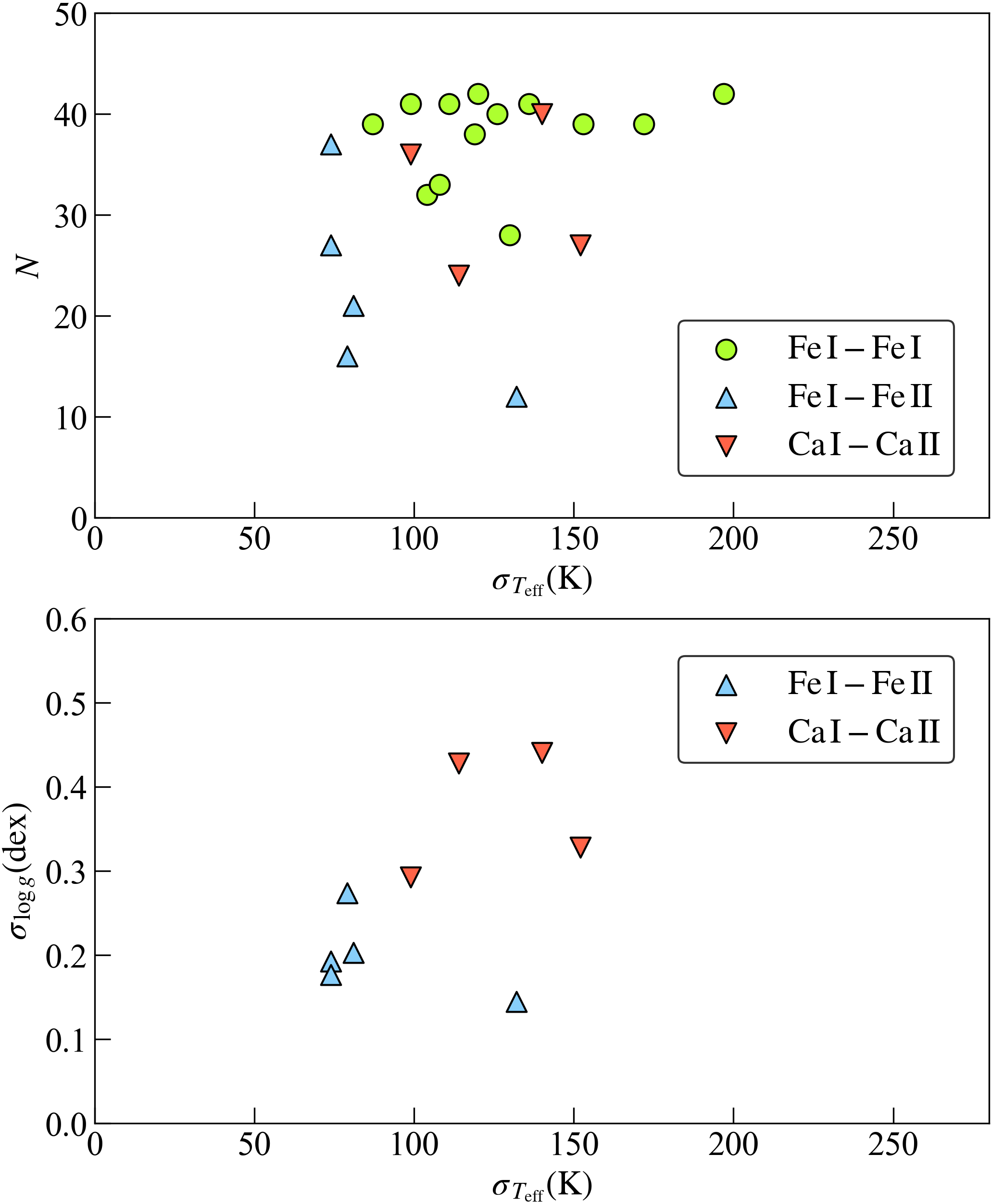
Figure 5: (Upper) The numbers, $N$, of the objects used for deriving the LDR relations (Table 3) are plotted against the residuals in ${T_{\mathrm{eff}}}$ ($\sigma_{{T_{\mathrm{eff}}}}$ in equation 3). (Lower) The residuals in $\log g$ ($\sigma_{\log g}$ in equation 6) are plotted against $\sigma_{{T_{\mathrm{eff}}}}$.

In our relations with the $\log g$ term (TG1–TG4), $\gamma$ indicates the LDR’s sensitivity to the surface gravity. This can be compared with the $\log g$ dependency detected by Jian et al. (2020). They measured the offsets in $\log r$, measured at a certain ${T_{\mathrm{eff}}}$, between dwarfs, giants and supergiants for dozens of relations of $YJ$-band LDRs given by Taniguchi et al. (2018). They found non-zero offsets in many line pairs, indicating significant impacts of surface gravity. In particular, the offsets between dwarfs and supergiants (corresponding to the difference of $\sim$3 dex in $\log g$) tend to be large, up to $\sim$0.6 dex, depending on the ionization potentials of the two elements in each line pair. Such dependency corresponds to $0\leq|\gamma|\lesssim 0.2$. Most of the six Fe i–Fe ii and Ca i–Ca ii pairs with the $y=\log r$ forms, common with the form in Jian et al. (2020), have $\gamma\sim 0.2$ or higher (the two smallest being 0.1588 and 0.1827). Among $\sim$40 line pairs for which the $\log g$ sensitivity was measured in Jian et al. (2020), only four show such high sensitivity. This comparison suggests that the pairs of neutral and ionized lines are indeed sensitive to $\log g$.

4 Discussion

4.1 Application of the LDR relations

In this section, we describe an application of the LDR relations to derive ${T_{\mathrm{eff}}}$ and $\log g$, and verify its performance. Due to the limited sample of available spectra, we apply the relations between the calibrators themselves in the subsequent analysis. This helps us check the self-consistency and provides an estimate of typical uncertainty. It is necessary to test the relations and evaluate the systematics on derived parameters, ${T_{\mathrm{eff}}}$ and $\log g$, by using a new dataset for different objects in the future.

The first step of the application procedure we propose is to use the Fe i–Fe i pairs for estimating ${T_{\mathrm{eff}}}$. We only consider the pairs of which the LDR ($y=r$ or $\log r$) is measured and validated for a given object. Let us suppose $N_{T}$ LDR values and their errors, $y_{j}\pm e_{j}$ ($1\leq j\leq N_{T}$), are available among the 13 Fe i–Fe i pairs in Table 3. For each LDR relation, $y_{j}=\alpha_{j}+\beta_{j}\,x$ (where $x={T_{\mathrm{eff}}}$ or $\log{T_{\mathrm{eff}}}$ according to the form selected for each line pair), we combine the scatter around the relation ($\sigma_{y}$ in equation 2) with the error in the measured LDR to give the error in $y_{j}$, i.e., $\varepsilon_{j}=\sqrt{e^{2}+\sigma_{y}^{2}}$. Then, we can estimate the effective temperature and its error with each individual LDR by

$$T_{j}\pm\Delta_{j}=\left\{\begin{array}[]{ll}(y_{j}-\alpha_{j})/\beta_{j}\pm\varepsilon_{j}/\beta_{j}&~{}({\rm if}~{}x={T_{\mathrm{eff}}})\\ 10^{(y_{j}-\alpha_{j})/\beta_{j}}\,\left[1\pm(\ln 10)\varepsilon_{j}/\beta_{j}\right]&~{}({\rm if}~{}x=\log{T_{\mathrm{eff}}}).\end{array}\right.$$ (10)

Then, we calculate the LDR-based temperature by taking the weighted mean of $T_{j}$:

$${T_{\mathrm{LDR}}}=\left.\sum_{j=1}^{N_{T}}\left(w_{j}T_{j}\right)\right/\sum_{j=1}^{N_{T}}w_{j},$$ (11)

where $w_{j}$ is the weight given by the error in equation (10). For the error in ${T_{\mathrm{LDR}}}$, we compare two kinds of errors:

$${\varepsilon_{\,T}}({\rm wav}) = \left(\frac{1}{N_{T}-1}\frac{\sum_{j=1}^{N_{T}}w_{j}\left(T_{j}-{T_{\mathrm{LDR}}}\right)^{2}}{\sum_{j=1}^{N_{T}}w_{j}}\right)^{1/2},$$ (12)

$${\varepsilon_{\,T}}({\rm prop}) = \left(\sum_{j=1}^{N_{T}}w_{j}\right)^{-1/2}.$$ (13)

The former is the weighted standard error, which reflects the dispersion of $T_{j}$, while the latter is the error propagated from the errors of $T_{j}$.

The second step is to estimate $\log g$ using the Fe i–Fe ii and Ca i–Ca ii pairs. $N_{G}$ denotes the number of these line pairs with LDR available. Some objects have $N_{G}$ less than 3, and we did not estimate their $\log\,{g_{\mathrm{LDR}}}$ (see Section 4.3). Each LDR relation in Table 3, $y_{j}=\alpha_{j}+\beta_{j}x_{j}+\gamma_{j}\log g$ where the assigned form determines $x_{j}={T_{\mathrm{eff}}}$ or $\log{T_{\mathrm{eff}}}$, leads to an estimate of $\log g$ for a given set of $x_{j}$ and $y_{j}$ ($1\leq j\leq N_{G}$). We again combine the measurement error and the residual around the relation to give the error in $y_{j}$, i.e., $\varepsilon_{j}=\sqrt{e^{2}+\sigma_{y}^{2}}$. If we assume the ${T_{\mathrm{eff}}}$ (leading to $x_{j}$) to be precise, the surface gravity and its error based on each line pair is given by

$$\log g_{j}=(y_{j}-\alpha_{j}-\beta_{j}x_{j})/\gamma_{j}\pm\varepsilon_{j}/\gamma_{j}.$$ (14)

We can calculate the weighted mean and its standard error ($\log{g_{\mathrm{LDR}}}\pm{\varepsilon_{G}}$), for the latter of which we considered the two kinds of error estimates like equations (12) and (13). We rejected estimates that deviated significantly from our parameter range, i.e., $\log g_{j}<0$ or $\log g_{j}>6$, and did not include them in calculating the weighted mean and the subsequent analysis. We rejected one or two $\log g_{j}$ for each of six objects (all having $\log g>3.5$ dex in Table 1). We could have done a similar rejection of the temperature estimates by equation (10) if $T_{j}<4000$ or $T_{j}>7500$, but none of the $T_{j}$ was rejected. In estimating $\log g_{j}$, ionized lines (Fe ii and Ca ii) tend to be rather weak especially in dwarfs, and very large errors may be observed in the estimation.

The error in the temperature, if not negligible, has a systematic effect on the LDR-based surface gravity. $\beta$ is negative in all the relations, and an overestimation of ${T_{\mathrm{eff}}}$ would result in a positive shift of $\log g_{j}$ from every line pair, and vice versa. The error in the temperature, ${\varepsilon_{\,T}}$, translates to the error in $x$,

$$\varepsilon_{x}=\left\{\begin{array}[]{ll}{\varepsilon_{\,T}}&~{}({\rm if}~{}x={T_{\mathrm{eff}}})\\ (\ln 10)^{-1}\,{\varepsilon_{\,T}}/{T_{\mathrm{eff}}}&~{}({\rm if}~{}x=\log{T_{\mathrm{eff}}})\end{array}\right..$$ (15)

The systematic error in the LDR-based $\log g$ due to the temperature error is then given by

$${\delta_{G}}=\left.\sum_{j=1}^{N_{G}}\left(-w_{j}\beta_{j}\varepsilon_{x}/\gamma_{j}\right)\right/\sum_{j=1}^{N_{G}}w_{j}$$ (16)

where the weights, $w_{j}=1/\varepsilon_{j}^{2}$, of individual line pairs are the ones used for deriving $\log{g_{\mathrm{LDR}}}$ (equation 14).

Table 4 lists the derived ${T_{\mathrm{LDR}}}\,(\pm{\varepsilon_{\,T}})$ and $\log\,{g_{\mathrm{LDR}}}\,(\pm{\varepsilon_{G}}\pm{\delta_{G}})$ and their differences from the catalogue values, ${T_{\mathrm{cat}}}$ and $\log{g_{\mathrm{cat}}}$,

$$\Delta_{T} = {T_{\mathrm{LDR}}}-{T_{\mathrm{cat}}},$$ (17)

$$\Delta_{G} = \log\,{g_{\mathrm{LDR}}}-\log\,{g_{\mathrm{cat}}}.$$ (18)

Fig. 6 plots $\Delta_{T}$ and $\Delta_{G}$ against three stellar parameters, i.e., ${T_{\mathrm{eff}}}$, $\log g$ and ${\mathrm{[Fe/H]}}$. The weighted standard deviations, 64 K in $\Delta_{T}$ and 0.18 dex in $\Delta_{G}$, correspond to the half widths of the horizontal strips. There is no clear correlation between the deviations from catalogue values and the stellar parameters.

Table 4: List of the ${T_{\mathrm{eff}}}$ and $\log g$ derived with the LDR relations. The definitions of the parameters are given in the text.

Object	${T_{\mathrm{LDR}}}$	${\varepsilon_{\,T}}$	$N_{T}$	$\Delta_{T}$	$\log\,{g_{\mathrm{LDR}}}$	${\varepsilon_{G}}$	${\delta_{G}}$	$N_{G}$	$\Delta_{G}$
HD 194093	6291	73	10	$89$	1.73	0.26	0.11	7	$0.38$
HD 171635	6283	97	6	$82$	2.06	0.23	0.12	8	$0.28$
HD 102870	6163	53	12	$108$	4.25	0.14	0.10	9	$0.25$
HD 137107	6201	91	6	$164$	—	—	—	—	—
HD 115383	6060	54	10	$48$	4.46	0.14	0.14	9	$0.16$
HD 19373	6001	46	13	$38$	4.29	0.11	0.08	8	$0.09$
HD 39587	6103	58	10	$148$	4.85	0.12	0.15	6	$0.55$
HD 114710	6032	49	13	$78$	4.49	0.13	0.09	6	$0.19$
HD 34411	5845	41	12	$-45$	4.16	0.10	0.06	7	$-0.04$
HD 95128	5984	48	13	$97$	4.53	0.12	0.11	7	$0.23$
HD 72905	5910	56	11	$26$	4.39	0.21	0.10	6	$-0.01$
HD 141004	5896	51	13	$12$	4.15	0.10	0.13	7	$0.05$
HD 143761	5792	56	13	$-73$	4.22	0.26	0.13	7	$-0.08$
HD 117176	5451	65	13	$-160$	3.65	0.23	0.17	5	$-0.21$
HD 101501	5465	43	13	$-93$	4.32	0.17	0.08	3	$-0.18$
HD 204867	5526	56	13	$60$	1.58	0.08	0.13	9	$0.04$
HD 31910	5496	54	12	$55$	1.62	0.10	0.11	8	$0.05$
HD 92125	5381	39	13	$27$	2.09	0.10	0.07	7	$-0.13$
HD 26630	5312	67	12	$-25$	1.49	0.09	0.16	8	$-0.25$
HD 3421	5183	61	12	$-119$	1.43	0.13	0.13	8	$-0.45$
HD 74395	5185	41	13	$-79$	1.46	0.09	0.09	8	$0.05$
HD 10476	5237	58	13	$-5$	4.57	0.36	0.17	4	$0.27$
HD 159181	5157	38	13	$-63$	1.59	0.10	0.09	7	$0.09$
HD 68312	5011	38	12	$-79$	2.72	0.15	0.07	5	$0.02$
HD 78235	5104	39	12	$34$	3.12	0.22	0.08	8	$0.12$
HD 76813	5002	39	11	$-58$	2.49	0.11	0.09	6	$-0.14$
HD 62345	5009	36	13	$-23$	2.77	0.44	0.04	3	$0.16$
HD 34559	5065	37	12	$55$	2.76	0.12	0.07	5	$0.02$
HD 27348	4984	41	13	$-19$	3.04	0.16	0.11	3	$0.29$
HD 11559	5009	35	13	$32$	3.10	0.21	0.08	5	$-0.13$
HD 202109	4976	36	12	$0$	2.12	0.15	0.07	5	$0.22$
HD 27697	5003	36	12	$28$	2.81	0.14	0.07	4	$0.17$
HD 27371	4955	36	12	$-5$	2.78	0.21	0.04	5	$0.02$
HD 77912	4839	42	12	$-118$	1.45	0.11	0.12	6	$-0.30$
HD 99648	4938	36	12	$-4$	2.15	0.11	0.05	6	$-0.09$
HD 122064	5032	38	12	$95$	—	—	—	—	—
HD 28305	4938	36	12	$13$	2.68	0.14	0.06	5	$-0.04$
HD 219134	4910	37	12	$10$	—	—	—	—	—
HD 198149	4935	46	13	$77$	3.32	0.21	0.12	5	$0.03$
HD 19787	4907	36	12	$75$	3.01	0.15	0.07	4	$0.09$
HD 82106	4892	50	12	$65$	—	—	—	—	—
HD 79555	4714	81	12	$-89$	—	—	—	—	—

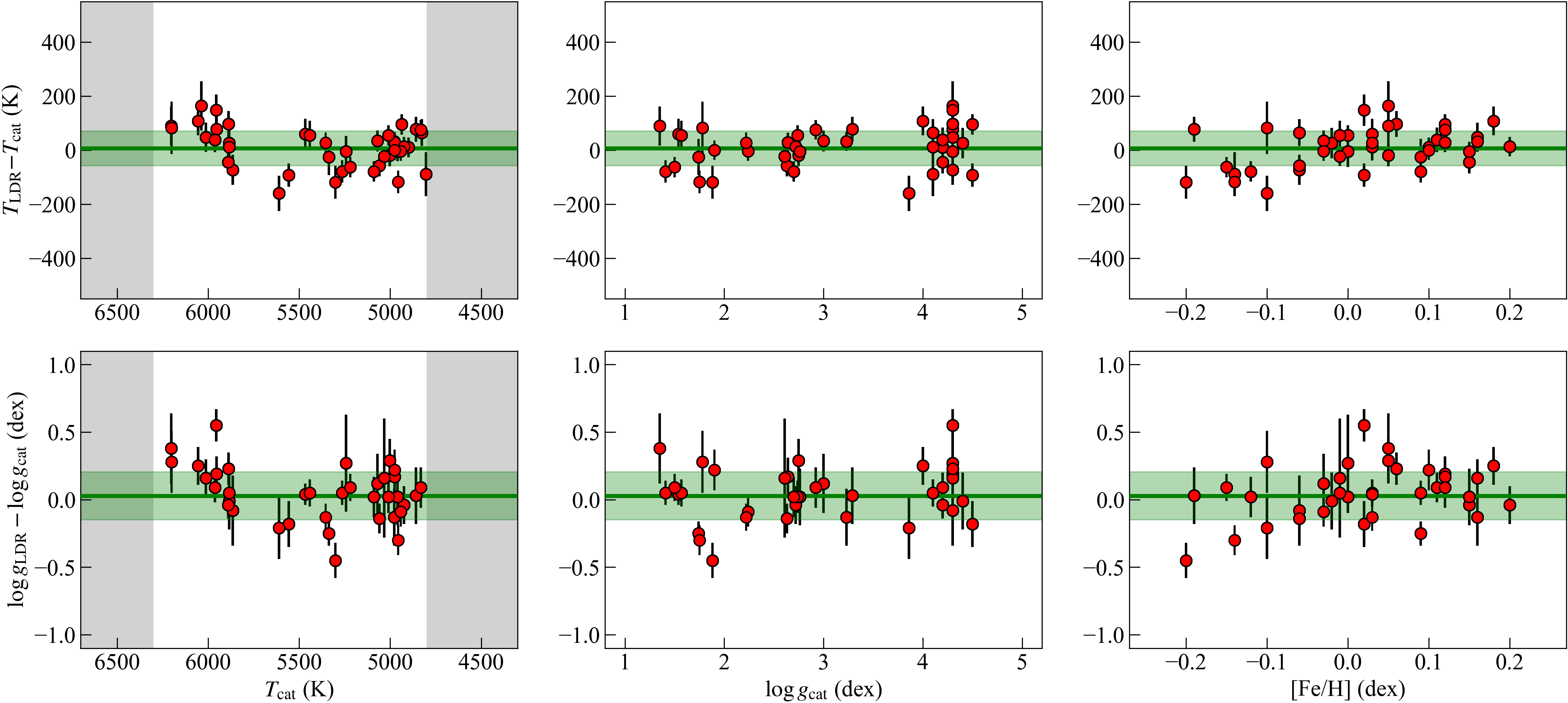
Figure 6: Plotted against three stellar parameters are $\Delta_{T}$ (upper panels) and $\Delta_{G}$ (lower panels). The horizontal strips indicate the weighted standard deviations, $\pm$42 K in $\Delta_{T}$ and $\pm$0.17 dex in $\Delta_{G}$.

Fig. 7 plots $\Delta_{T}/{\varepsilon_{\,T}}$ and $\Delta_{G}/\sqrt{{\varepsilon_{G}}^{2}+{\delta_{G}}^{2}}$ against the errors estimated with the LDR method. Roughly speaking, the deviations from the catalogue values are consistent with the scatter expected with the estimation errors. In the upper panel, 69 % and 88 % of the points are located within $\pm 1$ and $\pm 2$, respectively, while 75 % and 97 % are within $\pm 1$ and $\pm 2$ in the lower panel. The Gaussian error distribution would give 68 % and 95 % within $\pm 1$ and $\pm 2$. The estimated errors, i.e., ${\varepsilon_{\,T}}$ and $\sqrt{{\varepsilon_{G}}^{2}+{\delta_{G}}^{2}}$, seem to represent realistic uncertainties. The median of ${\varepsilon_{\,T}}$ in Table 4 is $\sim$45 K, while the median of $\sqrt{{\varepsilon_{G}}^{2}+{\delta_{G}}^{2}}$, is $\sim$0.18 dex.

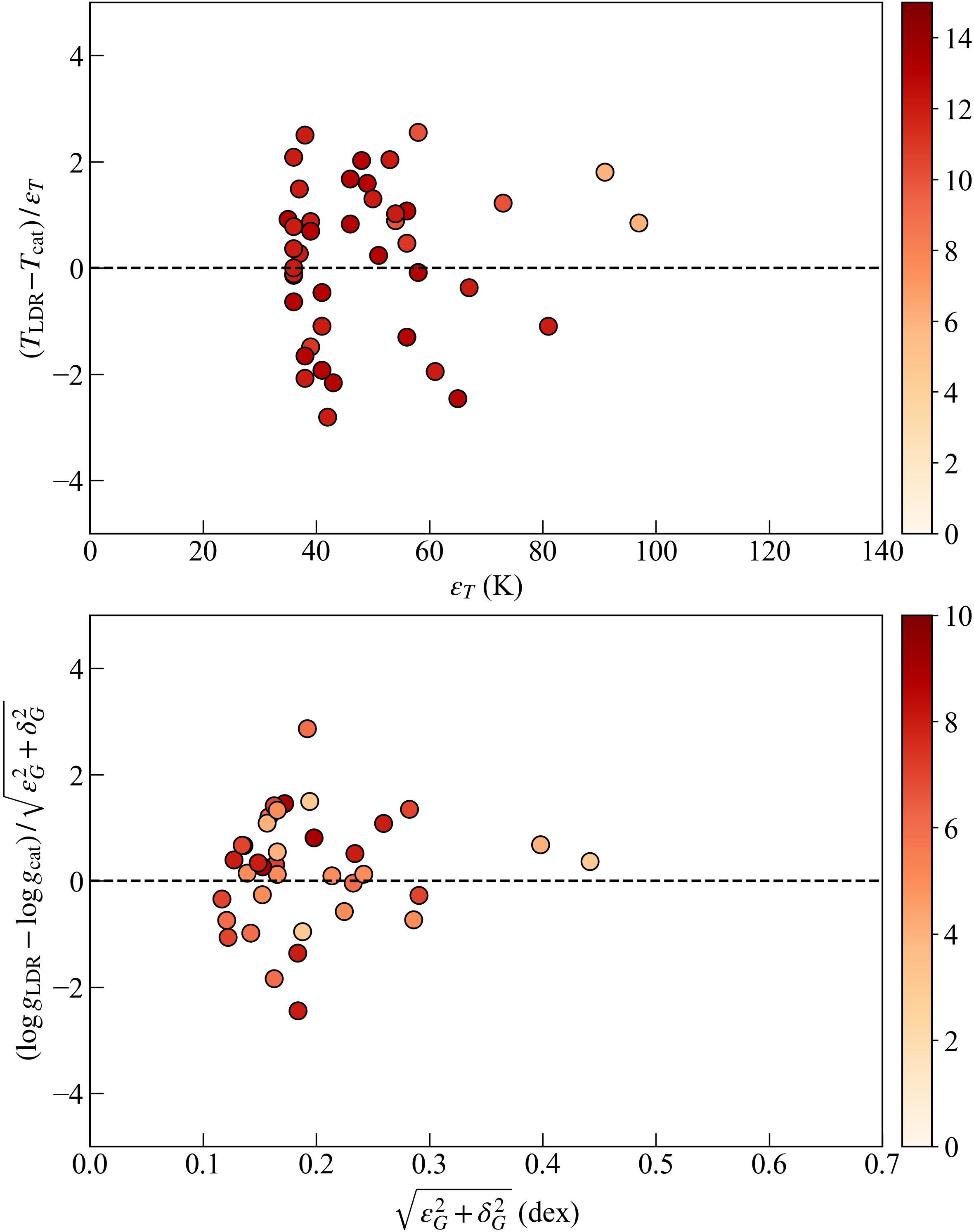
Figure 7: The differences between the LDR-based values and the catalogue values are compared with the estimated errors in the LDR-based values. The points’ colours indicate the numbers of line pairs used for the estimation.

4.2 Comparison with other gravity scales

In the previous section, we have examined the consistency and the internal precision of the method. However, the accuracy of the resultant $\log g$ scale depends entirely on the $\log g$ used for the calibration. The literature values we used were obtained with spectroscopic methods, and the balance between the neutral and ionized lines has an essential role in giving constraints on $\log g$. The previous works assumed that the approximations of LTE and hydrostatic equilibrium hold. These kinds of equilibrium have been questioned, and including the non-LTE effects has often modified and improved results of spectroscopic analysis (e.g., Asplund 2005; Bergemann et al. 2019; Amarsi et al. 2020; Bialek et al. 2020). Moreover, it has been demonstrated that significant non-LTE effects appear in some Fe lines (Bergemann et al., 2012) and Ca lines (Osorio et al., 2019) that are located within the wavelength range of our interest. Such non-canonical effects may be important for the LDR method if the stellar parameters for the calibration are affected by those effects. In Section 3.1, we used synthetic spectra with the equilibrium assumed for selecting the candidates of lines to use, but such an assumption has no impact on the steps after this selection because the calibration of the LDR relations is entirely empirical. However, if the literature values we used had systematic errors caused by the classical assumption of equilibrium, the current relations would lead to results affected by the same errors.

Here, we compare the $\log\,{g_{\mathrm{LDR}}}$ values with the surface gravities obtained using other studies for a sub-sample of the calibrators: 22 objects from Allende Prieto & Lambert (1999), 14 objects from Anders et al. (2019) and five objects from Gray & Kaur (2019). Allende Prieto & Lambert (1999) used the trigonometric parallaxes from the Hipparcos mission to put nearby stars within 100 pc from the Sun on the $(B-V)$–$M_{V}$ plane and compared their positions with the evolutionary models of Bertelli et al. (1994). Although these observational and theoretical data can be replaced with more up-to-date sets, their results give the largest sample for the comparison. Anders et al. (2019) obtained the stellar parameters together with the distance and interstellar extinction by comparing the broad-band magnitudes from Gaia DR2 and other large photometric surveys with the theoretical values based on the PAdova and TRieste Stellar Evolution Code (PARSEC; Bressan et al., 2012) and the synthetic stellar spectra (Kurucz, 1993). These two works, i.e. Allende Prieto & Lambert (1999) and Anders et al. (2019), are photometry-based. In contrast, Gray & Kaur (2019) took a spectroscopic approach to estimate ${T_{\mathrm{eff}}}$ and $\log g$, together, of 26 G and early K-type stars (dwarfs and giants) by comparing the observed and theoretical equivalent widths of Ni i, V i, Fe i and Fe ii lines (10 lines in total). Their lines are well-characterized and situated within a narrow range of the optical regime 6224–6266 Å. As far as $\log g$ is concerned, the solutions in their analysis were obtained by postulating that the stellar abundances derived with Fe ii agree with those derived with the neutral lines.

Fig. 8 presents the comparison of $\log\,{g_{\mathrm{LDR}}}$ with the $\log\,{g_{\mathrm{cat}}}$ from Allende Prieto & Lambert (1999), Anders et al. (2019) and Gray & Kaur (2019). Using our errors for the weights, $w=({\varepsilon_{G}}^{2}+{\delta_{G}}^{2})^{-1}$, the weighted means ($\mu_{\Delta}$) and standard deviations ($\sigma_{\Delta}$) of the differences from the literature values are as follows: $\mu_{\Delta}=0.07$ dex and $\sigma_{\Delta}=0.24$ dex in comparison with Allende Prieto & Lambert (1999), and $\mu_{\Delta}=-0.13$ dex and $\sigma_{\Delta}=0.43$ dex in comparison with Gray & Kaur (2019). In the case of Anders et al. (2019), their catalogue lists errors in $\log g$, some of which are as large as our errors. Therefore, we combined these errors in quadrature and obtained $\mu_{\Delta}=0.26$ dex and $\sigma_{\Delta}=0.27$ dex. Although we cannot rule out the systematic trends between the sets of $\log g$ obtained from different studies, our $\log\,{g_{\mathrm{LDR}}}$ values are found to be similar to the surface gravity scales in the literature, within $\sim$0.2 dex, across a wide range over 3 dex in $\log g$. The reasonable agreement of our values with both photometry- and spectroscopy-based results in the literatures indicates that the systematic error in our $\log g$ scale is not enormous.

Two objects show relatively large offsets. HD 202109 ($\zeta$ Cyg, with ${T_{\mathrm{eff}}}=4976$ K and $\log g=1.90$ dex in Table 1) is a spectroscopic binary with a white dwarf companion (Dominy & Lambert, 1983; Griffin & Keenan, 1992). We obtained $\log\,{g_{\mathrm{LDR}}}=2.12$ dex. It is slightly higher than the value in Table 1 taken from Luck (2014) and 1.98 dex by Anders et al. (2019), but lower than 2.51 dex by Allende Prieto & Lambert (1999) and 3.0 dex in Gray & Kaur (2019). HD 171635 (d Dra or 45 Dra) has ${T_{\mathrm{eff}}}=6201$ K and $\log g=1.78$ dex in Table 1. Our value, 2.06 dex, is higher than the value in Table 1 taken from Luck (2014) and 0.99 dex by Anders et al. (2019). We used five and eight line pairs (among the nine Fe i–Fe ii and Ca i–Ca ii pairs in Table 3) for HD 202109 and HD 171635, respectively, and the estimates with individual line pairs agree with each other for each object. It is unclear how the large deviations took place, and their true $\log g$ values need to be established.

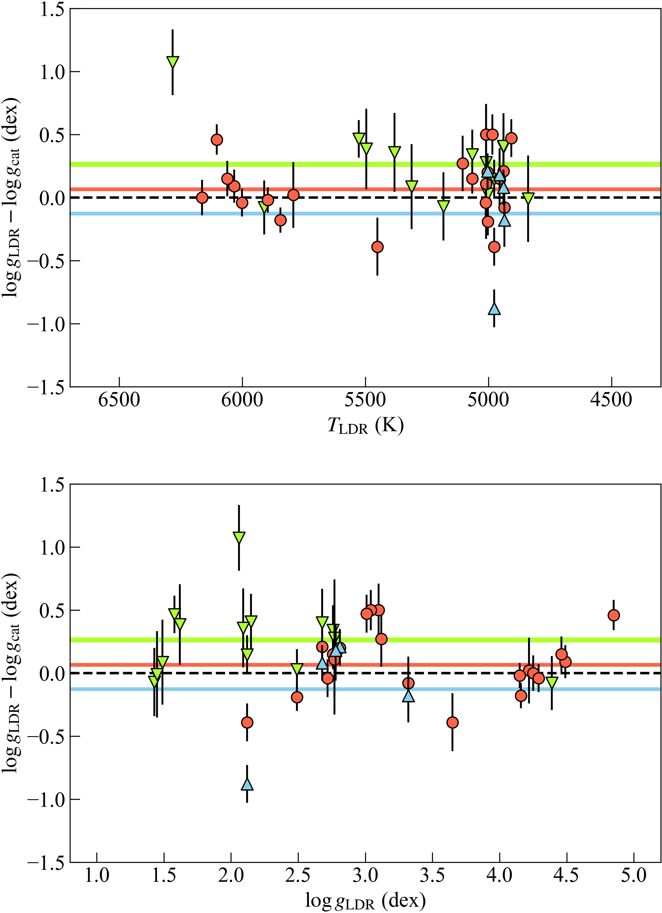
Figure 8: Comparison of the LDR-based surface gravities with $\log g$ obtained by Allende Prieto & Lambert (1999, indicated by blue upright triangles), Anders et al. (2019, green upside-down triangles) and Gray & Kaur (2019, red circles). The differences from the literature values are plotted against ${T_{\mathrm{LDR}}}$ in the upper panel and against $\log\,{g_{\mathrm{LDR}}}$ in the lower panel. Horizontal solid lines indicate the weighted means ($\mu_{\Delta}$) of the differences from the literature values (given in Section 4.2), and the dashed line merely indicates the zero difference.

4.3 Expected targets

Our method requires both neutral and ionized lines of each element to be visible in a given star. This requirement is satisfied only in stars with the spectral types around G. Fig. 9 represents the numbers of the line pairs we could use for deriving ${T_{\mathrm{LDR}}}$ (upper panel) and $\log\,{g_{\mathrm{LDR}}}$ (lower panel). The isochrones for four different ages (30 Myr, 100 Myr, 1 Gyr and 10 Gyr) are included to illustrate what kinds of stars can be the targets of our relations. We generated these isochrones for the solar metallicity using the CMD 3.4 tool for which the PARSEC models are used (Bressan et al., 2012). We include evolutionary stages up to early asymptotic giant branch (E-AGB), i.e. the thermally pulsing and post-AGB stages are not included. The upper panels of Fig. 9 shows that $T_{\rm LDR}$ was derived for all the 42 objects. As mentioned in Section 3.4.1, we required that every line pair gives the LDRs measured for the four groups, the groups (a) to (d) in Fig. 2, across the HRD. In the highest temperature range (${T_{\mathrm{eff}}}\gtrsim 6000$ K), the numbers of the LDRs tend to be small because Fe i lines get weak. In contrast, we could not derive $\log\,{g_{\mathrm{LDR}}}$ of five objects indicated by the crosses in the lower panel of Fig. 9, because the available LDRs are less than 3 for them. Towards the low ${T_{\mathrm{eff}}}$ end (${T_{\mathrm{eff}}}\lesssim 5250$ K), Fe ii lines become weak, especially among the higher-$\log g$ objects. Three of them are located above the main sequence, where no star is expected. Their $\log g$ are taken from Kovtyukh, Soubiran, & Belik (2004), while some recent references give higher values, $\log g\simeq 4.6$, consistent with the isochrones (e.g., Soubiran et al., 2016). Most of the ionized lines (Fe ii and Ca ii) were not measured well for these objects, and they have no significant impact on the calibration of our relations. On the other hand, the warm dwarf at ${T_{\mathrm{eff}}}>6000$ K lacking $\log\,{g_{\mathrm{LDR}}}$ is HD 137107, the double-lined binary mentioned in Section 2. In the case of this object, the large FWHM (Section 3.2) in combination with its relatively high ${T_{\mathrm{eff}}}$ prevents us from measuring some lines among both neutral and ionized ones.

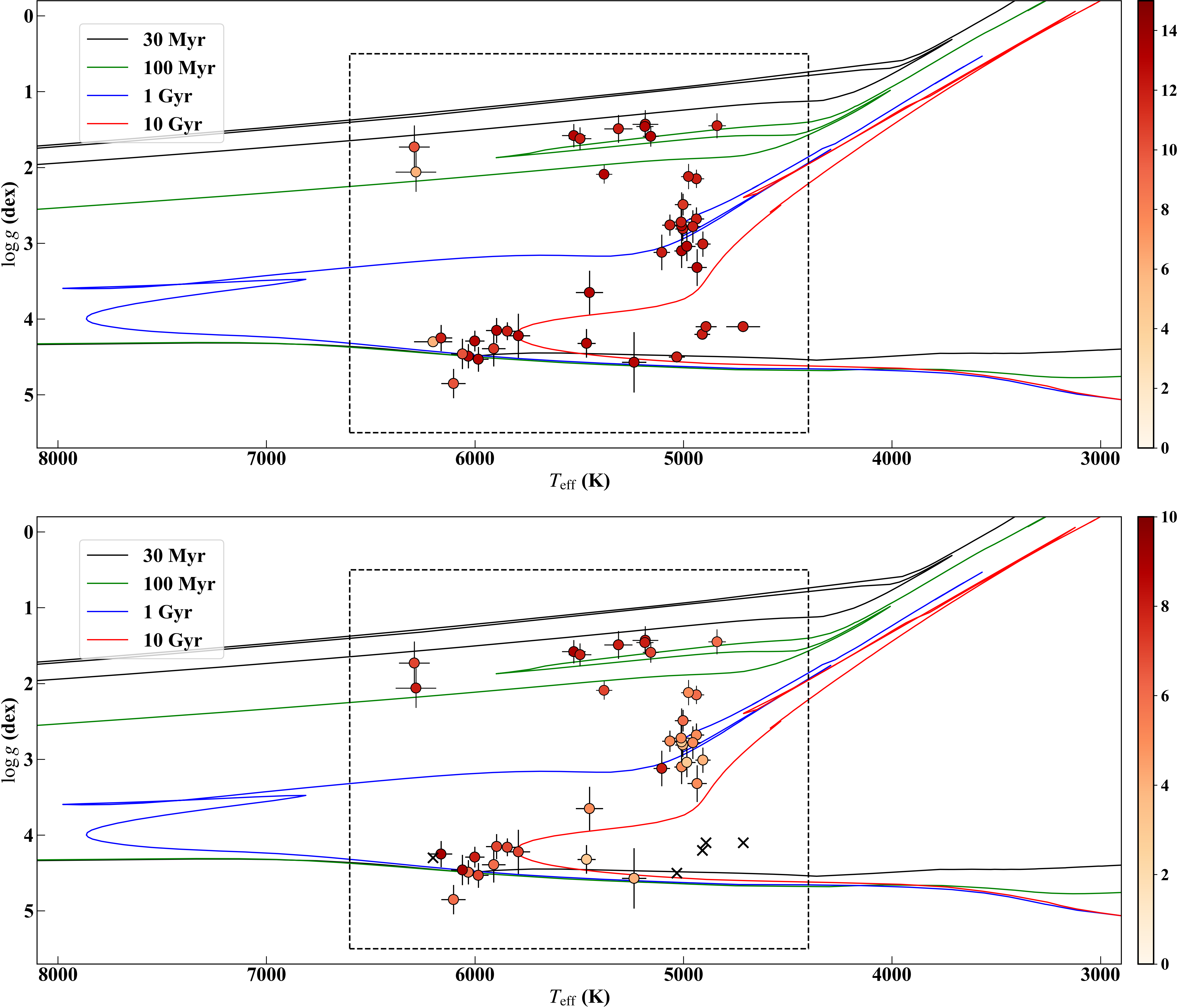
Figure 9: Locations of ${T_{\mathrm{eff}}}$ and $\log g$ derived with the LDR relations. The colour of circles indicates the number of used line pairs, i.e., Fe i–Fe i pairs ($N_{T}$) in the upper panel and Fe i–Fe ii plus Ca i–Ca ii pairs ($N_{G}$) in the lower panel. As presented in the upper panel, ${T_{\mathrm{eff}}}$ were derived with $N_{T}\geq 5$ for all the objects. In contrast, $\log g$ was not derived if $N_{G}$ is smaller than 3, and such objects are indicated by crosses in the lower panel. The isochrones for four different ages are drawn (see more details in text), and the dashed rectangle indicates the range covered in Fig. 2.

Unfortunately, the ${T_{\mathrm{eff}}}$ range in which both neutral and ionized lines appear is narrow. For Fe i–Fe ii and Ca i–Ca ii pairs, our examination of $YJ$-band spectra including synthetic ones indicates that the LDRs of these pairs are useful at around 4800–6300 K only. This range corresponds to the spectral types of late F to early K, which roughly covers the Cepheid instability strip.

Pulsating stars in the instability strip, classical Cepheids and RR Lyrs in particular, are useful tracers of the Galactic chemical evolution (Beaton et al., 2018; Matsunaga et al., 2018). Our sample does not include any of these pulsating stars, and it is necessary to test how well our method works for them. For example, classical Cepheids have been used to measure the metallicity gradient of the Galactic disk (Genovali et al., 2014, 2015; da Silva et al., 2016). A vast majority of the previous spectroscopic analyses on Cepheids were done with optical spectra, but the application of infrared spectra has been initiated (Inno et al., 2019; Minniti et al., 2020). In the pioneering two papers, Cepheids’ stellar parameters were determined by searching for the best-matched synthetic spectra (Section 1). However, the infrared spectra of Cepheids are poorly reproduced compared to the optical spectra. In terms of the determined metallicities, for example, Inno et al. (2019) and Minniti et al. (2020) estimated the errors to be 0.15 dex and 0.20 dex, respectively, while the errors $\sim$0.1 dex or lower have been achieved with high-quality optical spectra (e.g., Luck et al., 2011; Genovali et al., 2013; Takeda et al., 2013). The analysis with infrared spectra of Cepheids need to be developed and tested more extensively. Recently, a large number of classical Cepheids have been discovered across a very large area of the disk (Chen et al., 2019; Dékány et al., 2019; Skowron et al., 2019). Many distant Cepheids at ${\gtrsim}4$ kpc are heavily reddened by interstellar dust. They tend to be rather faint in the optical range, but many of them are still bright in the infrared range. Therefore, developing methods of analysing the Cepheids’ infrared spectra is essential for future investigations on the emerging sample of dust-obscured Cepheids. We can also find other interesting objects in this temperature range, e.g., yellow supergiants (Neugent et al., 2010, 2012) and yellow hypergiants (de Jager, 1998), planet-hosting dwarfs with ${T_{\mathrm{eff}}}$ not far from that of the Sun (Ramírez, Meléndez, & Asplund, 2009; Adibekyan et al., 2013), etc.

5 Conclusions

In near-infrared high-resolution spectra (0.97–1.32 $\mu$m with $\lambda/\Delta\lambda=28\,000$) of 42 FGK stars, we have selected line pairs of Fe i–Fe i, Fe i–Fe ii and Ca i–Ca ii combinations whose LDRs show tight relations with ${T_{\mathrm{eff}}}$ and $\log g$. Their simple linear relations allow us to predict ${T_{\mathrm{eff}}}$ and $\log g$ with a moderate precision (50 K and 0.2 dex) for late F to early K type stars (mainly G-type ones) in a wide range of luminosity class (from supergiants to dwarfs). This method does not require complex calculations with numerical models like the inference of chemical abundances. The current analysis suggests that the metallicity effect on the derived ${T_{\mathrm{eff}}}$ and $\log g$ is negligible, at least, within the metallicity range, $-0.2<{\mathrm{[Fe/H]}}<0.2$ dex, covered by our sample, although this independency and the ${\mathrm{[Fe/H]}}$ range of application need to be tested with larger datasets. We used simple linear formulae given in Section 3.4.1 and 3.4.2 considering the limited number and the non-uniform distribution of calibrators. Using a larger sample for calibration would allow us to try higher-order or more complex formulae, and this may reduce the fitting residuals. Moreover, it will be essential to improve the calibration by observing stars with accurate and precise $\log g$ known. In particular, objects with asteroseismic $\log g$ are very nice calibrators (e.g., Morel & Miglio 2012; Hekker et al. 2013; Pinsonneault et al. 2018), and empirical LDR relations would enable us to obtain surface gravities consistent with the asteroseismic estimates without introducing the systematic errors caused in the spectroscopic analysis such as the LTE/non-LTE difference.

Data Availability

The data underlying this article will be shared on a reasonable request with the corresponding author.

Supporting Information

Supplementary data are available at MNRAS online.

Table 2. List of the 97 confirmed lines that are used in search of line-depth ratio pairs (see Section 3.3). The last column lists the number of objects for which the depth measurements were validated. Among these lines, Ca ii 9890.6280 includes two transitions with $\log{gf}=0.900$ and $1.013$ at the same EP in VALD. Our electric table lists the combined strength ($\log{gf}=1.261$) with the “*” mark.

Figure 3. The relation between LDR ($r$ or $\log r$) and effective temperature (${T_{\mathrm{eff}}}$ or $\log{T_{\mathrm{eff}}}$) for the 13 Fe i–Fe i pairs in Table 3.

Figure 4. The relation between LDR ($r$ or $\log r$), effective temperature (${T_{\mathrm{eff}}}$ or $\log{T_{\mathrm{eff}}}$) and the surface gravity ($\log g$) for the 5 Fe i–Fe ii and 4 Ca i–Ca ii pairs in Table 3.

Table 2: The entire part of Table 2 available in Supporting Information. List of the 97 confirmed lines that are used to search line-depth ratio pairs (see Section 3.3). The last column lists the number of objects for which the depth measurements were validated. Fe i, Fe ii, Ca i and Ca ii lines are combined together. The first 10 lines are presented here, and the full table is available in Supporting Information.

Species	$\lambda_{\mathrm{air}}$	EP	$\log{gf}$ (dex)		$N_{\mathrm{obj}}$
	(Å)	(eV)	VALD	MB99
Fe i	9800.3075	5.086	$-0.453$	—	37
Fe i	9811.5041	5.012	$-1.362$	—	41
Fe i	9861.7337	5.064	$-0.142$	—	42
Fe i	9868.1857	5.086	$-0.979$	—	42
Fe i	9889.0351	5.033	$-0.446$	—	41
Fe i	9944.2065	5.012	$-1.338$	—	40
Fe i	9980.4629	5.033	$-1.379$	—	42
Fe i	10041.472	5.012	$-1.772$	$-1.84$	37
Fe i	10065.045	4.835	$-0.289$	$-0.57$	40
Fe i	10081.393	2.424	$-4.537$	$-4.53$	33
Fe i	10114.014	2.759	$-3.692$	$-3.76$	39
Fe i	10145.561	4.795	$-0.177$	$-0.41$	42
Fe i	10155.162	2.176	$-4.226$	$-4.36$	40
Fe i	10167.468	2.198	$-4.117$	$-4.26$	41
Fe i	10195.105	2.728	$-3.580$	$-3.63$	42
Fe i	10216.313	4.733	$-0.063$	$-0.29$	42
Fe i	10218.408	3.071	$-2.760$	$-2.93$	42
Fe i	10227.994	6.119	$-0.354$	—	21
Fe i	10265.217	2.223	$-4.537$	$-4.67$	34
Fe i	10332.327	3.635	$-2.938$	$-3.15$	35
Fe i	10340.885	2.198	$-3.577$	$-3.65$	42
Fe i	10347.965	5.393	$-0.551$	$-0.82$	42
Fe i	10353.804	5.393	$-0.819$	$-1.09$	42
Fe i	10364.062	5.446	$-0.960$	$-1.19$	42
Fe i	10395.794	2.176	$-3.393$	$-3.42$	42
Fe i	10423.743	3.071	$-2.918$	$-3.13$	41
Fe i	10435.355	4.733	$-1.945$	$-2.11$	41
Fe i	10469.652	3.884	$-1.184$	$-1.37$	42
Fe i	10532.234	3.929	$-1.480$	$-1.76$	42
Fe i	10535.709	6.206	$-0.108$	—	42
Fe i	10555.649	5.446	$-1.108$	$-1.39$	39
Fe i	10577.139	3.301	$-3.136$	$-3.28$	41
Fe i	10611.686	6.169	$0.021$	$-0.09$	42
Fe i	10616.721	3.267	$-3.127$	$-3.34$	41
Fe i	10674.070	6.169	$-0.466$	—	39
Fe i	10717.806	5.539	$-0.436$	$-1.68$	22
Fe i	10725.185	3.640	$-2.763$	$-2.98$	41
Fe i	10753.004	3.960	$-1.845$	$-2.14$	40
Fe i	10780.694	3.237	$-3.289$	$-3.59$	39
Fe i	10783.050	3.111	$-2.567$	$-2.80$	42
Fe i	10818.274	3.960	$-1.948$	$-2.23$	42
Fe i	10849.465	5.539	$-1.444$	$-0.73$	41
Fe i	10863.518	4.733	$-0.895$	$-1.06$	42
Fe i	10881.758	2.845	$-3.604$	$-3.50$	37
Fe i	10884.262	3.929	$-1.925$	$-2.18$	40

Table 2: — continued.

Species	$\lambda_{\mathrm{air}}$	EP	$\log{gf}$ (dex)		$N_{\mathrm{obj}}$
	(Å)	(eV)	VALD	MB99
Fe i	11607.572	2.198	$-2.009$	$-2.46$	41
Fe i	11638.260	2.176	$-2.214$	$-2.59$	41
Fe i	11689.972	2.223	$-2.068$	$-2.67$	37
Fe i	11783.265	2.832	$-1.574$	$-1.86$	42
Fe i	11882.844	2.198	$-1.668$	$-2.20$	42
Fe i	11884.083	2.223	$-2.083$	$-2.45$	42
Fe i	11973.046	2.176	$-1.483$	$-2.28$	42
Fe i	12053.082	4.559	$-1.543$	$-1.75$	41
Fe i	12119.494	4.593	$-1.635$	$-1.88$	39
Fe i	12190.098	3.635	$-2.330$	$-2.75$	39
Fe i	12213.336	4.638	$-1.845$	$-2.09$	38
Fe i	12227.112	4.607	$-1.368$	$-1.60$	42
Fe i	12283.298	6.169	$-0.537$	$-0.61$	39
Fe i	12342.916	4.638	$-1.463$	$-1.68$	28
Fe i	12556.996	2.279	$-3.626$	$-4.07$	41
Fe i	12615.928	4.638	$-1.517$	$-1.77$	40
Fe i	12638.703	4.559	$-0.783$	$-1.00$	41
Fe i	12648.741	4.607	$-1.140$	$-1.32$	41
Fe i	12789.450	5.010	$-1.514$	$-1.92$	37
Fe i	12807.152	3.640	$-2.452$	$-2.76$	35
Fe i	12808.243	4.988	$-1.362$	$-1.87$	26
Fe i	12824.859	3.018	$-3.835$	$-3.68$	28
Fe i	12840.574	4.956	$-1.329$	$-1.76$	36
Fe i	12879.766	2.279	$-3.458$	$-3.61$	35
Fe i	12896.118	4.913	$-1.424$	$-1.80$	30
Fe i	12934.666	5.393	$-0.948$	$-1.28$	41
Fe i	13006.684	2.990	$-3.744$	$-3.49$	41
Fe i	13014.841	5.446	$-1.693$	$-1.68$	38
Fe i	13039.647	5.655	$-0.731$	$-1.32$	27
Fe i	13098.876	5.010	$-1.290$	$-1.73$	34
Fe i	13147.920	5.393	$-0.814$	$-0.93$	42
Fe ii	9997.5980	5.484	$-1.867$	—	27
Fe ii	10173.515	5.511	$-2.736$	$-2.79$	13
Fe ii	10366.167	6.724	$-1.825$	$-1.76$	16
Fe ii	10501.500	5.549	$-2.086$	$-2.17$	40
Fe ii	10862.652	5.589	$-2.199$	$-2.11$	23
Ca i	10343.819	2.933	$-0.300$	$-0.40$	42
Ca i	10516.156	4.744	$-1.438$	$-0.52$	41
Ca i	10838.970	4.878	$0.238$	$0.03$	42
Ca i	10846.792	4.744	$-1.318$	$-0.64$	41
Ca i	11767.481	4.532	$-0.536$	$-0.80$	32
Ca i	11955.955	4.131	$-0.849$	$-0.91$	41
Ca i	12105.841	4.554	$-0.305$	$-0.54$	41
Ca i	12823.867	3.910	$-0.997$	$-1.34$	25
Ca i	12909.070	4.430	$-0.224$	$-0.50$	42
Ca i	13033.554	4.441	$-0.064$	$-0.31$	42
Ca i	13134.942	4.451	$0.085$	$-0.14$	33
Ca ii	9854.7588	7.505	$-0.205$	—	26
Ca ii	9890.6280	8.438	1.261∗	—	27
Ca ii	9931.3741	7.515	$0.092$	—	28
Ca ii	11838.997	6.468	$0.312$	$0.24$	40
Ca ii	11949.744	6.468	$0.006$	$-0.04$	39

Here presented are individual plots for Figure 3 which are available as the online material.

Here presented are individual plots for Figure 3 which are available as the online material.

Here presented are individual plots for Figure 3 which are available as the online material.

Here presented are individual plots for Figure 4 which are available as the online material.

Here presented are individual plots for Figure 4 which are available as the online material.

References

- Adibekyan et al. (2013) Adibekyan V. Z., Figueira P., Santos N. C., Mortier A., Mordasini C., Delgado Mena E., Sousa S. G., et al., 2013, A&A, 560, A51
- Allende Prieto & Lambert (1999) Allende Prieto C., Lambert D. L., 1999, A&A, 352, 555
- Allende Prieto et al. (2014) Allende Prieto C., Fernández-Alvar E., Schlesinger K. J., Lee Y. S., Morrison H. L., Schneider D. P., Beers T. C., et al., 2014, A&A, 568, A7
- Allende Prieto et al. (2006) Allende Prieto C., Beers T. C., Wilhelm R., Newberg H. J., Rockosi C. M., Yanny B., Lee Y. S., 2006, ApJ, 636, 804
- Amarsi et al. (2020) Amarsi A. M., Lind K., Osorio Y., Nordlander T., Bergemann M., Reggiani H., Wang E. X., et al., 2020, A&A, 642, A62
- Anders et al. (2019) Anders F., Khalatyan A., Chiappini C., Queiroz A. B., Santiago B. X., Jordi C., Girardi L., et al., 2019, A&A, 628, A94
- Andreasen et al. (2016) Andreasen D. T., Sousa S. G., Delgado Mena E., Santos N. C., Tsantaki M., Rojas-Ayala B., Neves V., 2016, A&A, 585, A143
- Asplund (2005) Asplund M., 2005, ARA&A, 43, 481
- Beaton et al. (2018) Beaton R. L., Bono G., Braga V. F., Dall’Ora M., Fiorentino G., Jang I. S., Martínez-Vázquez C. E., et al., 2018, SSRv, 214, 113
- Bergemann et al. (2012) Bergemann M., Kudritzki R.-P., Plez B., Davies B., Lind K., Gazak Z., 2012, ApJ, 751, 156
- Bergemann et al. (2019) Bergemann M., Gallagher A. J., Eitner P., Bautista M., Collet R., Yakovleva S. A., Mayriedl A., et al., 2019, A&A, 631, A80
- Bertelli et al. (1994) Bertelli G., Bressan A., Chiosi C., Fagotto F., Nasi E., 1994, A&AS, 106, 275
- Bialek et al. (2020) Bialek S., Fabbro S., Venn K. A., Kumar N., O’Briain T., Yi K. M., 2020, MNRAS, 498, 3817
- Bressan et al. (2012) Bressan A., Marigo P., Girardi L., Salasnich B., Dal Cero C., Rubele S., Nanni A., 2012, MNRAS, 427, 127
- Caffau et al. (2019) Caffau E., Bonifacio P., Oliva E., Korotin S., Capitanio L., Andrievsky S., Collet R., et al., 2019, A&A, 622, A68
- Catanzaro (2014) Catanzaro G., 2014, Determination of Atmospheric Parameters of B-, A-, F- and G-Type Stars. Springer International Publishing (Chambridge), eds. E. Niemczura, B. Smalley and W. Pych, 97
- Chaplin & Miglio (2013) Chaplin W. J., Miglio A., 2013, ARA&A, 51, 353
- Chen et al. (2019) Chen X., Wang S., Deng L., de Grijs R., Liu C., Tian H., 2019, NatAs, 3, 320
- da Silva, Milone, & Rocha-Pinto (2015) da Silva R., Milone A. de C., Rocha-Pinto H. J., 2015, A&A, 580, A24
- da Silva et al. (2016) da Silva R., Lemasle B., Bono G., Genovali K., McWilliam A., Cristallo S., Bergemann M., et al., 2016, A&A, 586, A125
- de Jager (1998) de Jager C., 1998, A&ARv, 8, 145
- Dékány et al. (2019) Dékány I., Hajdu G., Grebel E. K., Catelan M., 2019, ApJ, 883, 58
- Dominy & Lambert (1983) Dominy J. F., Lambert D. L., 1983, ApJ, 270, 180
- Duquennoy, Mayor, & Halbwachs (1991) Duquennoy A., Mayor M., Halbwachs J.-L., 1991, A&AS, 88, 281
- Follert et al. (2014) Follert R., Dorn R. J., Oliva E., Lizon J. L., Hatzes A., Piskunov N., Reiners A., et al., 2014, SPIE, 9147, 914719
- Fuhrmann et al. (1997) Fuhrmann K., Pfeiffer M., Frank C., Reetz J., Gehren T., 1997, A&A, 323, 909
- Fukue et al. (2015) Fukue K., Matsunaga N., Yamamoto R., Kondo S., Kobayashi N., Ikeda Y., Hamano S., et al., 2015, ApJ, 812, 64
- Fukue et al. (2021) Fukue K., Matsunaga N., Kondo S., Taniguchi D., Ikeda Y., Kobayashi N., Sameshima H., et al., 2021, ApJ, 913, 62
- García Pérez et al. (2016) García Pérez A. E., Allende Prieto C., Holtzman J. A., Shetrone M., Mészáros S., Bizyaev D., Carrera R., et al., 2016, AJ, 151, 144
- Genovali et al. (2013) Genovali K., Lemasle B., Bono G., Romaniello M., Primas F., Fabrizio M., Buonanno R., et al., 2013, A&A, 554, A132
- Genovali et al. (2014) Genovali K., Lemasle B., Bono G., Romaniello M., Fabrizio M., Ferraro I., Iannicola G., et al., 2014, A&A, 566, A37
- Genovali et al. (2015) Genovali K., Lemasle B., da Silva R., Bono G., Fabrizio M., Bergemann M., Buonanno R., et al., 2015, A&A, 580, A17
- Gray (2005) Gray D. F., 2005, The Observation and Analysis of Stellar Photospheres, Cambridge, UK, Cambridge University Press
- Gray & Johanson (1991) Gray D. F., Johanson H. L., 1991, PASP, 103, 439
- Gray & Kaur (2019) Gray D. F., Kaur T., 2019, ApJ, 882, 148
- Griffin & Keenan (1992) Griffin R. F., Keenan P. C., 1992, Obs, 112, 168
- Hekker et al. (2013) Hekker S., Elsworth Y., Mosser B., Kallinger T., Basu S., Chaplin W. J., Stello D., 2013, A&A, 556, A59
- Ikeda et al. (2016) Ikeda Y., Kobayashi N., Kondo S., Otsubo S., Hamano S., Sameshima H., Yoshikawa T., et al., 2016, SPIE, 9908, 99085Z
- Inno et al. (2019) Inno L., Urbaneja M. A., Matsunaga N., Bono G., Nonino M., Debattista V. P., Sormani M. C., et al., 2019, MNRAS, 482, 83
- Jian, Matsunaga, & Fukue (2019) Jian M., Matsunaga N., Fukue K., 2019, MNRAS, 485, 1310
- Jian et al. (2020) Jian M., Taniguchi D., Matsunaga N., Kobayashi N., Ikeda Y., Yasui C., Kondo S., et al., 2020, MNRAS, 494, 1724
- Kondo et al. (2019) Kondo S., Fukue K., Matsunaga N., Ikeda Y., Taniguchi D., Kobayashi N., Sameshima H., et al., 2019, ApJ, 875, 129
- Korn, Shi, & Gehren (2003) Korn A. J., Shi J., Gehren T., 2003, A&A, 407, 691
- Kotani et al. (2018) Kotani T., Tamura M., Nishikawa J., Ueda A., Kuzuhara M., Omiya M., Hashimoto J., et al., 2018, SPIE, 10702, 1070211
- Kovtyukh & Andrievsky (1999) Kovtyukh V. V., Andrievsky S. M., 1999, A&A, 351, 597
- Kovtyukh (2007) Kovtyukh V. V., 2007, MNRAS, 378, 617
- Kovtyukh et al. (2003) Kovtyukh V. V., Soubiran C., Belik S. I., Gorlova N. I., 2003, A&A, 411, 559
- Kovtyukh, Soubiran, & Belik (2004) Kovtyukh V. V., Soubiran C., Belik S. I., 2004, A&A, 427, 933
- Kovtyukh et al. (2006) Kovtyukh V. V., Soubiran C., Bienaymé O., Mishenina T. V., Belik S. I., 2006, MNRAS, 371, 879
- Kurucz (1993) Kurucz, R. 1993, ATLAS Stellar Atmosphere Programs and 2 km/s grid. Kurucz CD-ROM No. 13 (Cambridge, Mass.: Smithsonian Astrophysical Observatory), 13
- Liu et al. (2014) Liu Y. J., Tan K. F., Wang L., Zhao G., Sato B., Takeda Y., Li H. N., 2014, ApJ, 785, 94
- Luck et al. (2011) Luck R. E., Andrievsky S. M., Kovtyukh V. V., Gieren W., Graczyk D., 2011, AJ, 142, 51
- Luck (2014) Luck R. E., 2014, AJ, 147, 137
- Marfil et al. (2020) Marfil E., Tabernero H. M., Montes D., Caballero J. A., Soto M. G., González Hernández J. I., Kaminski A., et al., 2020, MNRAS, 492, 5470
- Matsunaga et al. (2018) Matsunaga N., Bono G., Chen X., de Grijs R., Inno L., Nishiyama S., 2018, SSRv, 214, 74
- Matsunaga et al. (2020) Matsunaga N., Taniguchi D., Jian M., Ikeda Y., Fukue K., Kondo S., Hamano S., et al., 2020, ApJS, 246, 10
- Meléndez & Barbuy (1999) Meléndez J., Barbuy B., 1999, ApJS, 124, 527
- Mészáros et al. (2013) Mészáros S., Holtzman J., García Pérez A. E., Allende Prieto C., Schiavon R. P., Basu S., Bizyaev D., et al., 2013, AJ, 146, 133
- Minniti et al. (2020) Minniti J. H., Sbordone L., Rojas-Arriagada A., Zoccali M., Contreras Ramos R., Minniti D., Marconi M., et al., 2020, A&A, 640, A92
- Morel & Miglio (2012) Morel T., Miglio A., 2012, MNRAS, 419, L34
- Mortier et al. (2014) Mortier A., Sousa S. G., Adibekyan V. Z., Brandão I. M., Santos N. C., 2014, A&A, 572, A95
- Muterspaugh et al. (2010) Muterspaugh M. W., Hartkopf W. I., Lane B. F., O’Connell J., Williamson M., Kulkarni S. R., Konacki M., et al., 2010, AJ, 140, 1623
- Neugent et al. (2012) Neugent K. F., Massey P., Skiff B., Meynet G., 2012, ApJ, 749, 177
- Neugent et al. (2010) Neugent K. F., Massey P., Skiff B., Drout M. R., Meynet G., Olsen K. A. G., 2010, ApJ, 719, 1784
- Osorio et al. (2019) Osorio Y., Lind K., Barklem P. S., Allende Prieto C., Zatsarinny O., 2019, A&A, 623, A103
- Park et al. (2013) Park S., Kang W., Lee J.-E., Lee S.-G., 2013, AJ, 146, 73
- Pinsonneault et al. (2018) Pinsonneault M. H., Elsworth Y. P., Tayar J., Serenelli A., Stello D., Zinn J., Mathur S., et al., 2018, ApJS, 239, 32
- Prugniel, Vauglin, & Koleva (2011) Prugniel P., Vauglin I., Koleva M., 2011, A&A, 531, A165
- Pourbaix (2000) Pourbaix D., 2000, A&AS, 145, 215
- Pourbaix et al. (2004) Pourbaix D., Tokovinin A. A., Batten A. H., Fekel F. C., Hartkopf W. I., Levato H., Morrell N. I., et al., 2004, A&A, 424, 727
- Ramírez, Meléndez, & Asplund (2009) Ramírez I., Meléndez J., Asplund M., 2009, A&A, 508, L17
- Ryabchikova et al. (2015) Ryabchikova T., Piskunov N., Kurucz R. L., Stempels H. C., Heiter U., Pakhomov Y., Barklem P. S., 2015, Phys. Scr., 90, 054005
- Sameshima et al. (2018) Sameshima H., Matsunaga N., Kobayashi N., Kawakita H., Hamano S., Ikeda Y., Kondo S., et al., 2018, PASP, 130, 074502
- Shetrone et al. (2015) Shetrone M., Bizyaev D., Lawler J. E., Allende Prieto C., Johnson J. A., Smith V. V., Cunha K., et al., 2015, ApJS, 221, 24
- Skowron et al. (2019) Skowron D. M., Skowron J., Mróz P., Udalski A., Pietrukowicz P., Soszyński I., Szymański M. K., et al., 2019, Sci, 365, 478
- Sneden et al. (2021) Sneden C., Afşar M., Bozkurt Z., Topcu G. B., Özdemir S., Zeimann G. R., Froning C. S., et al., 2021, AJ, 161, 128. doi:10.3847/1538-3881/abd7ee
- Sneden et al. (2012) Sneden C., Bean J., Ivans I., Lucatello S., Sobeck J., 2012, MOOG: LTE line analysis and spectrum synthesis (ascl:1202.009)
- Soubiran et al. (2016) Soubiran C., Le Campion J.-F., Brouillet N., Chemin L., 2016, A&A, 591, A118
- Takeda et al. (2013) Takeda Y., Kang D.-I., Han I., Lee B.-C., Kim K.-M., 2013, MNRAS, 432, 769
- Taniguchi et al. (2018) Taniguchi D., Matsunaga N., Kobayashi N., Fukue K., Hamano S., Ikeda Y., Kawakita H., et al., 2018, MNRAS, 473, 4993
- Taniguchi et al. (2021) Taniguchi D., Matsunaga N., Jian M., Kobayashi N., Fukue K., Hamano S., Ikeda Y., et al., 2021, MNRAS, 502, 4210
- Tsantaki et al. (2019) Tsantaki M., Santos N. C., Sousa S. G., Delgado-Mena E., Adibekyan V., Andreasen D. T., 2019, MNRAS, 485, 2772