A Note on Optimizing Distributions
using Kernel Mean Embeddings

Abstract

Kernel mean embeddings are a popular tool that consists in representing probability measures by their infinite-dimensional mean embeddings in a reproducing kernel Hilbert space. When the kernel is characteristic, mean embeddings can be used to define a distance between probability measures, known as the maximum mean discrepancy (MMD). A well-known advantage of mean embeddings and MMD is their low computational cost and low sample complexity. However, kernel mean embeddings have had limited applications to problems that consist in optimizing distributions, due to the difficulty of characterizing which Hilbert space vectors correspond to a probability distribution. In this note, we propose to leverage the kernel sums-of-squares parameterization of positive functions of Marteau-Ferey et al. (2020) to fit distributions in the MMD geometry. First, we show that when the kernel is characteristic, distributions with a kernel sum-of-squares density are dense. Then, we provide algorithms to optimize such distributions in the finite-sample setting, which we illustrate in a density fitting numerical experiment.

1 Introduction

Mean embeddings (Muandet et al., 2017) are a way of representing probability distributions through the moments of a potentially infinite-dimensional feature vector, usually corresponding to the feature map $\phi(x)$ of a reproducing kernel Hilbert space (RKHS) ${\mathcal{H}}$. When this RKHS is large enough (i.e., when the kernel is characteristic (Sriperumbudur et al., 2011)) this embedding is injective, i.e., a distribution is uniquely characterized by its mean embedding. From there, one may define a distance between probability distributions as the distance between their embeddings in the Hilbert space, known as the maximum mean discrepancy (MMD) (Gretton et al., 2012).

MMD benefits from a low computational cost and a favorable sample complexity. More precisely, given two distributions $\mu,\nu$ on $\mathbb{R}^{d}$, one may get a estimate of the MMD distance based on $n$ samples from $\mu$ and $\nu$ with a precision $O(n^{-1/2})$, independently from the dimension $d$, at a $O(dn^{2})$ computational cost. For those reasons, MMD has become a popular distance in the machine learning community that has had applications to testing (Gretton et al., 2012; Sejdinovic et al., 2013) and generative modeling (Li et al., 2015; Bińkowski et al., 2018), among others.

However, numerous machine learning applications such as density fitting (Parzen, 1962; Silverman, 1986) or distributionally robust optimization (DRO) (Rahimian and Mehrotra, 2019) place the focus on optimizing distributions themselves. Despite its practical advantages, MMD has had limited applications to those tasks, due to the difficulty of characterizing which functions in a RKHS are the mean embeddings of a probability distribution. Indeed, while ${\mathcal{H}}$ corresponds to the space spanned by $\{\phi(x),x\in\mathbb{R}^{d}\}$, the set of mean embeddings ${\mathfrak{M}}$ is only the convex hull of this set, whose extreme points are the feature vectors $\phi(x),x\in\mathbb{R}^{d}.$ This can be related to the pre-image problem (Kwok and Tsang, 2004): given an element $v$ of ${\mathcal{H}}$, the pre-image problem consists in finding a point $x$ whose feature vector $\phi(x)$ is equal or close to $v$. In comparison, we aim here at finding a distribution $\mu$ such that $\mathbb{E}_{\mu}[\phi(x)]$ is close to $v$.

As a workaround, Staib and Jegelka (2019) propose to relax such problems by optimizing over any function in ${\mathcal{H}}$, instead of restricting to those in ${\mathfrak{M}}$. As a result, the output of those methods are not guaranteed to correspond to probability distributions: they may correspond to measures that do not have unit mass, or that take negative values. Alternatively, in some settings it is possible to obtain a tractable exact problem by deriving the dual (Zhu et al., 2021).

Contributions.

In this short note, we leverage the kernel sum-of-squares representation for positive functions proposed by Marteau-Ferey et al. (2020) to design a method to optimize over probability distributions in the MMD distance. In the finite-sample setting, this parameterization can be approximated with a finite-rank positive-semidefinite (PSD) matrix. Based on this fact, we provide algorithmic tools to solve optimization problems over distributions in the MMD geometry. Finally, we illustrate our methods on a density fitting example.

2 Background and notation

Notation.

For $n\in\mathbb{N},[n]$ denotes the set $\{1,...,n\}$. We use lower-case fonts for vectors (e.g., $v$), and bold upper-case fonts for matrices (e.g., $\mathbf{B}$). We denote inner products $\langle\cdot,\,\cdot\rangle$ to which we add a subscript: $F$ for the Frobenius product between matrices, ${\mathcal{H}}$ for the Hilbert inner product on ${\mathcal{H}}$, HS for the Hilbert-Schmidt product between bounded operators on ${\mathcal{H}}$. For a set $\mathcal{X}$, $\mathcal{P}(\mathcal{X})$ denotes the space of probability distributions on $\mathcal{X}$, and when applicable $\mathcal{AC}(\mathcal{X})$ is the subset of absolutely continuous probability distributions (i.e., that admit a density w.r.t. the Lebesgue measure on $\mathcal{X}$). $\mathcal{C}_{0}(\mathcal{X})$ denotes the set of real-valued continuous functions on $\mathcal{X}$ that vanish at infinity.

Kernels and reproducing kernel Hilbert spaces (RKHS).

We refer to Steinwart and Christmann (2008) and Paulsen and Raghupathi (2016) for a more complete covering of the subject. Let $\mathcal{X}$ be a set and $k:\mathcal{X}\times\mathcal{X}\mapsto\mathbb{R}$. $k$ is a positive-definite kernel if and only if for any set of points $x_{1},...,x_{n}\in\mathcal{X}$, the matrix of pairwise evaluations $K_{ij}=k(x_{i},x_{j}),i,j\in[n]$ is positive semi-definite. Given a kernel $k$, there exists a unique associated reproducing kernel Hilbert space (RKHS) ${\mathcal{H}}$, that is, a Hilbert space of functions from $\mathcal{X}$ to $\mathbb{R}$ satisfying the two following properties:

• For all $x\in\mathcal{X}$, $k_{x}\operatorname{\overset{\operatorname{def}}{=}}k(x,\cdot)\in{\mathcal{H}}$;

• For all $f\in{\mathcal{H}}$ and $x\in\mathcal{X}$, $f(x)=\langle f,\,k_{x}\rangle_{\mathcal{H}}$. In particular, for all $x,x^{\prime}\in\mathcal{X}$ it holds $\langle k_{x},\,k_{x^{\prime}}\rangle_{\mathcal{H}}=k(x,x^{\prime})$.

A feature map is a bounded map $\phi:\mathcal{X}\mapsto{\mathcal{H}}$ such that $\forall x,x^{\prime}\in\mathcal{X},\langle\phi(x),\,\phi(x^{\prime})\rangle_{\mathcal{H}}=k(x,x^{\prime})$. A particular instance is $x\mapsto k_{x}$, which is referred to as the canonical feature map. Many practical applications of RKHS theory can be cast as minimization problems of the form

$$\underset{f\in\mathcal{H}}{\min}~{}~{}L(f(x_{1}),...,f(x_{n}))+\Omega(\|f\|_{\mathcal{H}}),$$ (1)

where $\Omega:\mathbb{R}_{+}\mapsto\mathbb{R}$ is a strictly increasing function. In that case, the representer theorem (see, e.g., Steinwart and Christmann, 2008; Paulsen and Raghupathi, 2016, and references therein) shows that solutions of $\eqref{eq:generic_rkhs_pb}$ admit the following finite representation: $f=\sum_{i=1}^{n}\alpha_{i}k_{x_{i}}$ for some $\alpha\in\mathbb{R}^{n}$.

Kernel mean embeddings and maximum mean discrepancy (MMD).

Given a probability measure $\mu$, we define its kernel mean embedding as the element $w_{\mu}$ of ${\mathcal{H}}$ that satisfies $\forall f\in{\mathcal{H}},\,\mathbb{E}_{X\sim\mu}[f(x)]=\langle f,\,w_{\mu}\rangle_{\mathcal{H}}$, which may be expressed as $w_{\mu}=\int_{\mathcal{X}}\phi(x)\mathrm{d}\mu(x)$. When the kernel is characteristic (Sriperumbudur et al., 2011) – such as the Gaussian kernel – the embedding $\mu\mapsto w_{\mu}$ is injective. Note that mean embeddings are a strict subset of ${\mathcal{H}}$: as mentioned in Section 1, an element of ${\mathcal{H}}$ is the kernel mean embedding of a distribution if and only if it lies in ${\mathfrak{M}}\operatorname{\overset{\operatorname{def}}{=}}\operatorname{Conv}(\{\phi(x):x\in{\mathcal{H}}\})$, whereas ${\mathcal{H}}=\operatorname{Span}(\{\phi(x):x\in{\mathcal{H}}\})$. Using kernel mean embeddings, we may define a distance between probability measures, called the maximum mean discrepancy (Gretton et al., 2012):

$$\text{MMD}(\mu,\nu)\operatorname{\overset{\operatorname{def}}{=}}\|w_{\mu}-w_{\nu}\|_{\mathcal{H}}.$$

When $\nu$ admits a density $p$, we write by abuse $\text{MMD}(\mu,p)$ for $\text{MMD}(\mu,\nu)$.

2.1 Relaxing mean embedding constraints: a counter-example

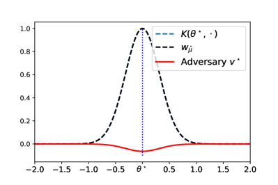
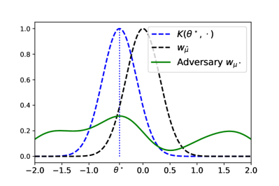
Figure 1: RKHS norm relaxation (left) vs. MMD solution (right). Note that the relaxed adversary (left) is not the mean embedding of a probability distribution (it is the embedding of a Dirac in $0$ with a negative mass). The solution of the unrelaxed problem is evaluated by discretizing the support interval [-2, 2], for which we obtain $\theta^{\star}\approx-0.4$. A equivalent symmetrical saddle point with $\theta^{\star}\approx 0.4$ also exists.

We conclude this section with a simple example to illustrate how replacing MMD constraints over distributions with RKHS norm constraints over vectors can be detrimental. Let $\hat{\mu}$ denote a distribution of observed data points, and $K$ a positive-definite translation-invariant kernel (e.g., the Gaussian kernel $K(x,y)=e^{-\frac{\|x-y\|^{2}}{\sigma^{2}}}$) with corresponding RKHS ${\mathcal{H}}$. Assume the convolution $(K\ast\hat{\mu})$ of $\hat{\mu}$ by $K$ denotes a “return function”, that a player wants to maximize by picking the highest mode:

$$\max_{\theta\in\mathbb{R}^{d}}~{}(K\ast\hat{\mu})(\theta).$$ (2)

The player knows that an adversary might have perturbed the data $\hat{\mu}$ that they have observed, compared to a true underlying distribution $\mu$ from which the player will get their returns. To hedge themselves against the adversary, the player decides to optimize $\theta$ over the worst distribution in a MMD ball around the observed distribution $\hat{\mu}$:

$$\max_{\theta\in\mathbb{R}^{d}}\min_{\mu\in\mathcal{P}(\mathbb{R}^{d})}(K\ast\mu)(\theta)~{}~{}~{}\text{s.t.}~{}~{}~{}\text{MMD}(\mu,\hat{\mu})\leq\varepsilon.$$ (3)

As mentioned in the introduction, problems of this form are generally intractable. As an example, Staib and Jegelka (2019) are confronted to this issue in applications to distributionally robust optimization, and propose to circumvent the difficulty by relaxing the problem: instead of restricting to distributions in the MMD distance, they optimize over ${\mathcal{H}}$ in the RKHS norm. Observing that the objective of eq. 3 can be rewritten as the inner product $(K\ast\mu)(\theta)=\langle w_{\mu},\,\phi(\theta)\rangle_{\mathcal{H}}$, this yields the following relaxed problem:

$$\max_{\theta\in\mathbb{R}^{d}}\min_{v\in{\mathcal{H}}}~{}~{}\langle v,\,\phi(\theta)\rangle_{\mathcal{H}}~{}~{}~{}\text{s.t.}~{}~{}~{}\|v-w_{\hat{\mu}}\|_{\mathcal{H}}\leq\varepsilon.$$ (4)

Equation 4 is a saddle point problem, in which the inner minimum a is convex problem. Writing the optimality conditions for the min, we get that the optimal adversary is $v^{\star}(\theta)=w_{\hat{\mu}}-\varepsilon\frac{\phi(\theta)}{\|\phi(\theta)\|}$. Plugging this back in eq. 4, the problem becomes

$$\max_{\theta\in\mathbb{R}^{d}}~{}(K\ast\hat{\mu})(\theta)-\varepsilon\sqrt{K(\theta,\theta)}.$$ (5)

Let us observe two things: first, in general $v^{\star}(\theta)$ is not the mean embedding of a probability distribution, and may even take negative values. Second, given that $K$ is a translation-invariant kernel, the solution $\theta^{\star}$ of eq. 5 is the same as the non-robust version (2) and does not depend on $\varepsilon$: only the value of the objective does. Hence, the relaxed version (4) fails at guaranteeing adversarial robustness. On the other hand, the original adversarial problem over distributions in eq. 3 does not admit a simple analytical expression, but does guarantee robustness against adversarial perturbations. This is illustrated in Figure 1 in a 1D case where $\hat{\mu}$ is a Dirac centered in 0 and $K$ is the Gaussian kernel. The discrepancy between the MMD geometry over distributions and the RKHS norm over general functions is already visible in this toy example. This suggests that the RKHS norm relaxation is ill-suited to more complex, higher-dimensional tasks and settings, and calls for better ways of dealing with optimization problems on distributions with MMD.

3 Optimizing over distributions using kernel sums-of-squares

As mentioned in Section 1, problems of the form

$$\inf_{\mu\in\mathcal{P}(\mathcal{X})}F(v)~{}~{}\text{s.t.}~{}v=\int\phi(x)\mathrm{d}\mu(x)$$ (6)

are notoriously difficult to tackle. In this note, we introduce a parametric model for smooth distributions that is compatible with MMD, that can be plugged in eq. 6. We focus on measures that admit a smooth density $p$ w.r.t. to a reference measure $\rho\in\mathcal{M}(\mathcal{X})$ (e.g., for $\mathcal{X}\subset\mathbb{R}^{d}$ we may consider the Lebesgue measure), and propose to represent such densities using the kernel sum-of-squares (SoS) representation of non-negative functions of Marteau-Ferey et al. (2020):

$$p_{A}(x)=\langle\phi(x),\,A\phi(x)\rangle_{\mathcal{H}},~{}~{}~{}x\in\mathcal{X},$$ (7)

with $A\in\mathbb{S}_{+}({\mathcal{H}})$. The following lemma (which is a particular case of Proposition 4 of Marteau-Ferey et al. (2020)) characterizes the operators $\mathbb{S}_{+}({\mathcal{H}})$ that lead to a valid density $p_{A}$ (i.e., with total mass equal to $1$). Its proof is deferred to the appendix.

Lemma 1.

Let $A\in\mathbb{S}_{+}({\mathcal{H}})$ and $\rho\in\mathcal{M}(\mathcal{X})$. Define $\Sigma_{\rho}\operatorname{\overset{\operatorname{def}}{=}}\int_{\mathcal{X}}\phi(x)\otimes\phi(x)\mathrm{d}\rho(x)$. The function $p_{A}$ defined in eq. 7 is a density w.r.t. $\rho$ if and only if $\langle A,\,\Sigma_{\rho}\rangle_{\text{HS}}=1$.

From there, we propose to handle problems of the form (6) using the parameterization in eq. 7, i.e., to solve

$$\inf_{A\in\mathbb{S}_{+}({{\mathcal{H}}})}F(w_{p_{A}})~{}~{}\text{s.t.}~{}~{}\mathrm{Tr}(A\Sigma_{\rho})=1.$$ (8)

We will denote $\mathcal{F}_{\rho}\operatorname{\overset{\operatorname{def}}{=}}=\{p_{A}:A\in\mathbb{S}_{+}({{\mathcal{H}}}),\mathrm{Tr}A\Sigma_{\rho}=1\}$. This representation has the double advantage of being parametric – and thus amenable to learning, as we will show in the remainder of this work – and universal. Indeed, as proved by Marteau-Ferey et al. (2020), any continuous positive function can be approximated arbitrarily well in maximum norm over compact subsets by a function of the form of eq. 7 provided ${\mathcal{H}}$ is large enough: this is referred to as universality (Micchelli et al., 2006).

Proposition 1 (Marteau-Ferey et al. (2020)).

Let ${\mathcal{H}}$ be a RKHS with a universal feature map $\phi:\mathcal{X}\mapsto\mathbb{R}^{d}$. Then $\{p_{A}:A\in\mathbb{S}_{+}({{\mathcal{H}}}),\mathrm{Tr}A<\infty\}$ is a universal approximator of continuous non-negative functions on $\mathcal{X}$.

In particular, this representation allows to approximate continuous density functions on $\mathcal{X}$ arbitrarily well. However, depending on the choice of topology, Proposition 1 alone does not guarantee that any distribution can be approximated by a distribution with a density in $\mathcal{F}_{\rho}$. For instance, in the total variation distance such densities may approach distributions with continuous density functions, but may not approach Dirac distributions. We show in the following theorem that distributions with densities in $\mathcal{F}_{\rho}$ are dense in the set of probability distributions for the weak topology. When the kernel is continuous (like most usual kernels) and when ${\mathcal{H}}\subset\mathcal{C}_{0}$, this implies in turn that $\mathcal{F}_{\rho}$ is dense for the MMD distance (Simon-Gabriel et al., 2020, Lemma 2.1).

Theorem 1.

Let $\mathcal{X}$ be a compact subset of $\mathbb{R}^{d}$, ${\mathcal{H}}$ be a RKHS with a universal feature map $\phi:\mathcal{X}\mapsto\mathbb{R}^{d}$, and assume $\rho$ is absolutely continuous. Then distributions with densities w.r.t. $\rho$ in $\mathcal{F}_{\rho}$ are dense in $\mathcal{P}(\mathcal{X})$ for the topology of the weak convergence.

Examples.

Kernels and RKHS satisfying the hypothesis of Proposition 1 and Theorem 1 include (but do not limit to):

• the Gaussian kernel $k(x,x^{\prime})=e^{-\frac{\|x-x^{\prime}\|^{2}}{\sigma^{2}}}$;

• the Laplace kernel $k(x,x^{\prime})=e^{-\frac{\|x-x^{\prime}\|}{\sigma}}$;

• more generally, the Sobolev kernels $k_{s}(x,x^{\prime})\propto\|x-x^{\prime}\|^{s-d/2}\mathcal{K}_{s-d/2}(\|x-x^{\prime}\|)$ with $s>d/2$ and where $\mathcal{K}_{s-d/2}$ is the Bessel function of the second kind, whose corresponding RKHS are the Sobolev spaces of smoothness $s$ (Adams and Fournier, 2003).

Finally, Hilbert space distances of mean embeddings with densities of the form eq. 7 (and MMD in particular) can be expressed as functions of $\phi$-tensors of order $4$:

Lemma 2.

Let $A\in\mathbb{S}_{+}({{\mathcal{H}}}),\mathrm{Tr}A<\infty$ and $v\in{\mathcal{H}}$. It holds

$$\|v-w_{p_{A}}\|^{2}_{\mathcal{H}}=\|v\|_{\mathcal{H}}^{2}+\langle A,\,\mathcal{T}(A)\rangle_{\text{HS}}-2\langle A,\,\mathcal{V}\rangle_{\text{HS}},$$ (9)

$$\text{with}~{}~{}\mathcal{V}\operatorname{\overset{\operatorname{def}}{=}}\int v(x)\phi(x)\otimes\phi(x)\mathrm{d}\rho(x)$$

$$\text{and}~{}~{}\mathcal{T}(A)\operatorname{\overset{\operatorname{def}}{=}}\iint\phi(x)\otimes\phi(x)\langle\phi(y),\,A\phi(y)\rangle_{\text{HS}}\,k(x,y)\mathrm{d}\rho(x)\mathrm{d}\rho(y)\ \in\ \mathbb{S}_{+}({{\mathcal{H}}}).$$

3.1 Low-rank representations

As recalled in Section 2, a key benefit of working in an RKHS is the existence of the representer theorem, which allows to learn functions from samples in a finite-dimensional representation. Marteau-Ferey et al. (2020) prove an extension of the representer theorem for kernel SoS of the form (7). More precisely, the solution of a problem of the form

$$\underset{A\in\mathbb{S}_{+}({{\mathcal{H}}})}{\min}L(p_{A}(x_{1}),...,p_{A}(x_{n}))+\lambda\mathrm{Tr}A$$ (10)

admits a representation of the form $A=\sum_{ij}^{n}B_{ij}\phi(x_{i})\otimes\phi(x_{j})$ with $\mathbf{B}\in\mathbb{S}_{+}({\mathbb{R}^{n}})$. However, unless $\Sigma_{\rho}$ admits a finite-rank parameterization, this result does not hold under the additional constraint $\langle A,\,\Sigma_{\rho}\rangle_{\text{HS}}=1$ that is required to ensure that $p_{A}$ is a density (Lemma 1).

As a workaround, we make an approximation and consider problems between vectors that are projected on a finite-dimensional subspace ${\mathcal{H}}_{m}=\operatorname{Span}\{\phi(\tilde{x}_{1}),...,\phi(\tilde{x}_{m})\}$ where $\tilde{x}_{1},...,\tilde{x}_{m}$ are a set of supporting points, and consider the case where $A\in\mathbb{S}_{+}({{\mathcal{H}}_{m}})$. In that case, we can write $A=\sum_{i=1}^{m}B_{ij}\phi(\tilde{x}_{i})\otimes\phi(\tilde{x}_{j})$ with $\mathbf{B}\in\mathbb{S}_{+}({\mathbb{R}^{m}})$, and we define $p_{\mathbf{B}}(x)=\sum_{ij=1}^{m}B_{ij}k(x,\tilde{x}_{i})k(x,\tilde{x}_{j})$. From Lemma 1, $p_{\mathbf{B}}$ is a valid density if and only if $\mathrm{Tr}(\mathbf{B}\mathbf{W})=1$ with $W_{ij}\operatorname{\overset{\operatorname{def}}{=}}\int_{\mathcal{X}}k(x,\tilde{x}_{i})k(x,\tilde{x}_{j})\mathrm{d}\rho(x),i,j\in[m]$. Let $P_{m}$ denote the orthogonal projection onto ${\mathcal{H}}_{m}$, i.e. $P_{m}(\phi(x))=\sum_{i=1}^{m}c_{i}\phi(\tilde{x}_{i})$ with $c=\tilde{\mathbf{K}}^{-1}\tilde{k}_{x}$ where $\tilde{K}_{ij}=k(\tilde{x}_{i},\tilde{x}_{j}),i,j\in[m]$ and $(\tilde{k}_{x})_{i}=k(x,\tilde{x}_{i}),i\in[m]$. In particular, for a function that admits a finite representation $v=\sum_{i=1}^{n}a_{i}\phi(x_{i})$, we have $P_{m}(v)=\sum_{i=1}^{m}b_{i}\phi(\tilde{x}_{i})$ with $b=\tilde{\mathbf{K}}^{-1}\mathbf{K}(\tilde{X},X)a$ and $\mathbf{K}(\tilde{X},X)_{ij}=k(\tilde{x}_{i},x_{j}),i\in[m],j\in[n]$. The following lemma gives a closed-form expression of the RKHS distance between a vector in ${\mathcal{H}}$ that admits a finite representation, and the mean embedding $w_{p_{\mathbf{B}}}$. Its proof is deferred to Appendix A.

Lemma 3.

Let $\mathbf{B}\in\mathbb{S}_{+}({\mathbb{R}^{m}})$ and $v=\sum_{i=1}^{n}a_{i}\phi(x_{i})$, and $W_{ij}\operatorname{\overset{\operatorname{def}}{=}}\int_{\mathcal{X}}k(x,\tilde{x}_{i})k(x,\tilde{x}_{j})\mathrm{d}\rho(x),i,j\in[m]$. For $p,q\in[m]$, denote $\mathbf{u}_{pq}=\int k(x,\tilde{x}_{p})k(x,\tilde{x}_{q})\tilde{k}_{x}\mathrm{d}\rho(x)\in\mathbb{R}^{m}$. Then, $p_{\mathbf{B}}$ is a density function if and only if $\mathrm{Tr}(\mathbf{B}\mathbf{W})=1$, and it holds

$$\|P_{m}(v-w_{p_{\mathbf{B}}})\|^{2}_{\mathcal{H}}=\mathcal{U}(\mathbf{B})^{T}\tilde{\mathbf{K}}^{-1}\mathcal{U}(\mathbf{B})-2\langle\mathbf{B},\,\mathbf{V}\rangle_{F}+\|P_{m}(v)\|_{\mathcal{H}}^{2},$$ (11)

with $\forall p,q\in[m],V_{pq}=\mathbf{u}_{pq}^{T}\tilde{\mathbf{K}}^{-1}\mathbf{K}(\tilde{X},X)a$, and $\mathcal{U}$ is the map from $\mathbb{R}^{m\times m}$ to $\mathbb{R}^{m}$ such that $\mathcal{U}(\mathbf{B})=\sum_{1\leq p,q\leq m}B_{pq}\mathbf{u}_{pq}$.

In particular, whenever the vectors $\mathbf{u}_{pq},p,q\in[m]$ are available in closed form (see examples in Appendix B), $\|P_{m}(v-w_{p_{\mathbf{B}}})\|^{2}_{\mathcal{H}}$ can be computed in $O(m^{3}+nm^{2})$ time.

3.2 Algorithms

We now provide algorithmic tools to optimize distributions with densities in $\mathcal{F}_{\rho}$. We illustrate those techniques on the sample problem of fitting a distribution with a kernel SoS density to observed data, with an optional trace regularization term:

$$\inf_{A\in\mathbb{S}_{+}({{\mathcal{H}}_{m}})}\|P_{m}(v-w_{p_{A}})\|^{2}_{\mathcal{H}}+\lambda\mathrm{Tr}A~{}~{}\text{s.t.}~{}~{}\mathrm{Tr}(A\Sigma_{\rho})=1.$$ (12)

Writing $A=\sum_{ij}B_{ij}\phi(\tilde{x}_{i})\otimes\phi(\tilde{x}_{j})$, we have $\mathrm{Tr}A=\sum_{ij}B_{ij}k(\tilde{x}_{i},\tilde{x}_{j})$. Hence, from Lemma 3 and ignoring terms that do not depend on $\mathbf{B}$, eq. 12 can be reformulated as

$$\inf_{\mathbf{B}\succeq 0}\mathcal{U}(\mathbf{B})^{T}\tilde{\mathbf{K}}^{-1}\mathcal{U}(\mathbf{B})-\langle\mathbf{B},\,2\tilde{\mathbf{V}}-\lambda\tilde{\mathbf{K}}\rangle_{F}~{}~{}\text{s.t.}~{}~{}\mathrm{Tr}(\mathbf{B}\mathbf{W})=1,$$ (13)

with $W_{ij}\operatorname{\overset{\operatorname{def}}{=}}\int_{\mathcal{X}}k(x,\tilde{x}_{i})k(x,\tilde{x}_{j})\mathrm{d}\rho(x),i,j\in[m]$. Equation 13 is a smooth convex optimization problem, and can therefore be solved using (accelerated) gradient descent. However, the projection on the set $\mathcal{A}\operatorname{\overset{\operatorname{def}}{=}}\{\mathbf{M}\in\mathbb{S}_{+}({\mathbb{R}^{m}}):\mathrm{Tr}(\mathbf{M}\mathbf{W})=1\}$ is computationally expensive (it is an instance of the covariance adjustment problem (Malick, 2004; Boyd and Xiao, 2005)). We circumvent this issue by changing the parameterization to $\mathbf{C}=\mathbf{R}\mathbf{B}\mathbf{R}^{T}$, where $\mathbf{R}$ satisfies $\mathbf{W}=\mathbf{R}^{T}\mathbf{R}$ (e.g., the Cholesky factor of $\mathbf{W}$). With this parameterization, we have

$$\mathbf{B}\in\mathcal{A}\iff\mathbf{C}\in\mathcal{B}\operatorname{\overset{\operatorname{def}}{=}}\{\mathbf{M}\in\mathbb{S}_{+}({\mathbb{R}^{m}}):\mathrm{Tr}(\mathbf{M})=1\},$$

with the advantage that the projection on $\mathcal{B}$ is much easier to compute: see Algorithm 1. This projection relies on computing the eigenvalue decomposition of $\mathbf{C}$ (in $O(m^{3})$ time) followed by the projection of its eigenvalues on the simplex in $O(m)$ time (Maculan and de Paula Jr, 1989). With this parameterization, eq. 13 becomes

$$\inf_{\mathbf{C}\succeq 0}\mathcal{U}(\mathbf{R}^{-1}\mathbf{C}\mathbf{R}^{-T})^{T}\tilde{\mathbf{K}}^{-1}\mathcal{U}(\mathbf{R}^{-1}\mathbf{C}\mathbf{R}^{-T})+\langle\mathbf{C},\,\mathbf{R}^{-T}(\lambda\tilde{\mathbf{K}}-2\mathbf{V})\mathbf{R}^{-1}\rangle_{F}~{}~{}\text{s.t.}~{}~{}\mathrm{Tr}(\mathbf{C})=1.$$ (14)

We may optimize this objective using projected gradient descent, or FISTA (Beck and Teboulle, 2009). The initial formation of $\mathbf{V}$, $\mathbf{R}^{-1}$ and $\mathbf{u}_{pq},p,q\in[m]$ has a $O(mn+m^{3})$ computational cost, and $O(mn+m^{3})$ memory footprint. From then, each (accelerated) projected gradient iteration has complexity $O(m^{3})$ and $O(m^{3})$ memory footprint (since storing $\mathbf{K}(\tilde{X},X)$ is not necessary once $\mathbf{V}$ is formed). Hence, using FISTA eq. 13 can be minimized to precision $\varepsilon$ with a total $O\left(mn+\frac{m^{3}}{\varepsilon^{2}}\right)$ computational cost (Beck and Teboulle, 2009, Theorem 4.4).

Algorithm 1 Projection on $\mathcal{B}$

0:  $\mathbf{X}\in\mathrm{Sym}({\mathbb{R}^{n}})$

  Compute the EVD of $\mathbf{X}$: $\mathbf{X}=\mathbf{U}\operatorname{diag}(\lambda_{1},...,\lambda_{n})\mathbf{U}^{T}$.

  Project on the simplex: $(\lambda_{1},...,\lambda_{n})_{+}\leftarrow\mathrm{proj}_{\Delta_{n}}(\lambda_{1},...,\lambda_{n})$,   $\Delta_{n}\operatorname{\overset{\operatorname{def}}{=}}\{x\in\mathbb{R}_{+}^{n}:\sum_{i=1}^{n}x_{i}=1\}$

  $\mathbf{X}_{+}=\mathbf{U}\operatorname{diag}(\lambda_{1},...,\lambda_{n})_{+}\mathbf{U}^{T}$

Remark 1.

Depending on the choice of kernel parameters, eq. 13 and eq. 14 may have poor conditioning. In particular, forming the Cholesky decomposition $\mathbf{W}=\mathbf{R}^{T}\mathbf{R}$ and inverting $\mathbf{R}$ may suffer from numerical stability issues. While a classical way of dealing with such issues is to use pre-conditioning (Rudi et al., 2017) on $\mathbf{B}$, this approach is not compatible with the projection strategy described in Algorithm 1. As an alternative, when the conditioning is problematic we propose to add a small diagonal term to $\mathbf{W}$ and to apply the constraint $\mathrm{Tr}(\mathbf{B}(\mathbf{W}+\lambda\mathbf{I}))=1$, and then renormalize $\mathbf{B}$ to satisfy Lemma 1: $\mathbf{B}\leftarrow\frac{\mathbf{B}}{1-\lambda\mathrm{Tr}\mathbf{B}}$.

4 Applications and numerical experiments

Motivated by Theorem 1, we propose to handle problems of the form (6) using our parameterization, i.e., to solve

$$\inf_{A\in\mathbb{S}_{+}({{\mathcal{H}}})}F(w_{p_{A}})~{}~{}\text{s.t.}~{}~{}\mathrm{Tr}(A\Sigma_{\rho})=1.$$ (15)

Example 1: density fitting.

Given $n$ points $x_{1},...,x_{n}$ sampled from an unknown distribution $\mu$, density fitting (Parzen, 1962) aims at estimating a parametric model $\mu_{\theta}$ for $\mu$ based on its samples. Motivated by Theorem 1, we propose to fit a density estimator $p_{\mathbf{B}}\in\mathcal{F}_{\rho}$ using MMD, with an optional regularization term:

$$\min_{\mathbf{B}\succeq 0}~{}~{}\text{MMD}(\frac{1}{n}\sum_{i=1}^{n}\delta_{x_{i}},p_{\mathbf{B}})+\lambda\mathrm{Tr}\mathbf{B}\mathbf{K}~{}~{}\text{such that}~{}~{}\mathrm{Tr}(\mathbf{B}\mathbf{W})=1.$$ (16)

Example 2: distributionally robust optimization.

Kernel distributionally robust optimization (DRO) (Staib and Jegelka, 2019; Zhu et al., 2021) consists in minimizing a loss function $\ell_{f}$ over $f\in{\mathcal{H}}$ under bounded adversarial perturbations of the input data $\hat{\mu}=\sum_{i=1}^{n}\delta_{x_{i}}$:

$$\begin{split}\min_{f\in{\mathcal{H}}}\max_{\mu\in\mathcal{P}(\mathcal{X})}&\mathbb{E}_{x\sim\mu}[\ell_{f}(x)]~{}~{}\text{s.t.}~{}~{}\text{MMD}(\mu,\hat{\mu})\leq\varepsilon.\end{split}$$ (17)

Due to the difficulty of optimizing under the constraint $\text{MMD}(\mu,\hat{\mu})\leq\varepsilon$, several relaxations of this problem have been proposed, leading to problems that do not respect the MMD geometry, as illustrated in Section 2.1. We propose instead to perform DRO with the parameterization (15). Problem (17) then becomes

$$\begin{split}\min_{f\in{\mathcal{H}}}\max_{\mathbf{B}\in\mathbb{S}_{+}({\mathbb{R}^{n}})}&\sum_{i,j=1}^{n}B_{ij}\int\ell_{f}(x)k(x,x_{i})k(x,x_{j})\mathrm{d}\rho(x)\\ \textrm{subject to}~{}~{}~{}&\mathrm{Tr}(\mathbf{B}\mathbf{W})=1~{}~{}\text{and}~{}~{}\text{MMD}(\hat{\mu},p_{\mathbf{B}})\leq\varepsilon.\end{split}$$ (18)

Provided $\ell_{f}$ is convex in $f$, (17) is a convex-concave min-max problem. Hence, whenever the integral $\int\ell_{f}(x)k(x,x_{i})k(x,x_{j})\mathrm{d}\rho(x)$ can be computed in closed form (e.g., for the square loss with a Gaussian kernel), eq. 17 can be solved using standard min-max optimization techniques.

Numerical experiments.

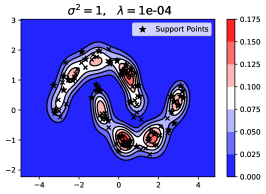
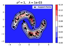
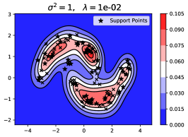
(a) Effect of regularization.

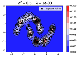
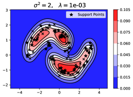
(b) Effect of bandwidth.

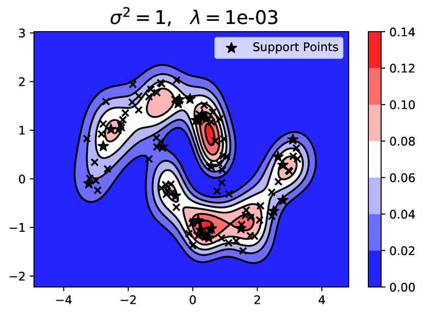
$m=25$

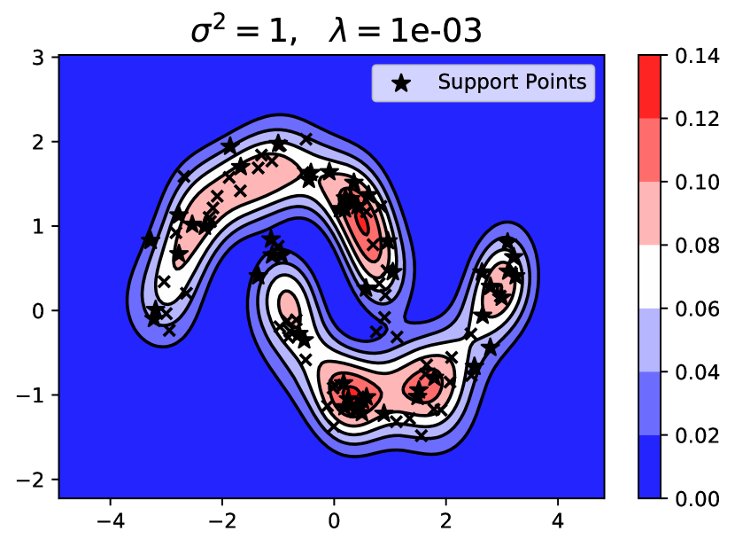
$m=50$

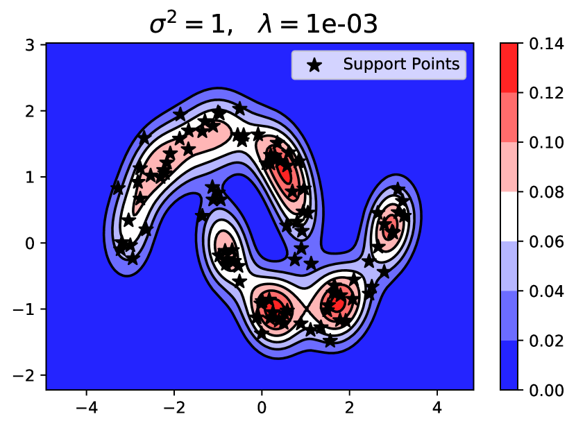
$m=100$

(c) Effect of sample size v.s. support size: $m$ out of $n=100$ supporting points are sampled.

We provide numerical results of a 2D density fitting task. We leave to future work the implementation of more complex applications, such as the DRO problem described above. In Figures 2(a), 2(b) and 2(c), we sample $n=100$ points from a “two moons” distribution, out of which $m$ points are used as support points $\tilde{x}_{1},...,\tilde{x}_{m}$, and minimize eq. 16 using the Gaussian kernel. In Figures 2(a) and 2(b), we fix $m=50$ and we illustrate the effect of bandwidth v.s. trace regularization, while in Figure 2(c) we show the impact of varying the support size $m$. The code to reproduce these figures is available at https://github.com/BorisMuzellec/kernel-SoS-distributions.

Conclusion and future work

In this note, we proposed to represent smooth probability distributions using kernel sums-of-squares as a way to address the intractability of optimizing distributions in the MMD geometry. We showed that this representation is dense for the weak topology, and can therefore be used to approximate arbitrarily well the solution of such problems on the whole space of probability measures. Finally, we provided efficient algorithms to fit kernel sum-of-squares densities. We leave to future work the application of this model to more complex tasks, such as distributionally robust optimization.

Appendix A Appendix

A.1 Proof of Lemma 1

Proof.

By definition it holds $\forall x\in\mathcal{X},p_{A}(x)\geq 0$. Hence, $p_{A}$ is a density if and only if $\int_{\mathcal{X}}p_{A}(x)\mathrm{d}\rho(x)=1$. We have

$$\int_{\mathcal{X}}p_{A}(x)\mathrm{d}\rho(x) =\int_{\mathcal{X}}\langle\phi(x),\,A\phi(x)\rangle_{\mathcal{H}}\mathrm{d}\rho(x)$$

$$=\langle A,\,\int_{\mathcal{X}}\phi(x)\otimes\phi(x)\mathrm{d}\rho(x)\rangle_{\text{HS}}$$

$$=\langle A,\,\Sigma_{\rho}\rangle_{\text{HS}},$$

where $\langle\cdot,\,\cdot\rangle_{\text{HS}}$ denotes the Hilbert-Schmidt inner product, and the operator $\Sigma_{\rho}\operatorname{\overset{\operatorname{def}}{=}}\int_{\mathcal{X}}\phi(x)\otimes\phi(x)\mathrm{d}\rho(x)$ is well-defined from the assumption $\sup_{x\in\mathcal{X}}k(x,x)<\infty$. ∎

A.2 Proof of Theorem 1

Proof.

We consider w.l.o.g. the case where $\rho$ is the Lebesgue measure on $\mathcal{X}$. Since $\mathcal{AC}(\mathcal{X})$ is dense in $\mathcal{P}(\mathcal{X})$ for the weak topology, it suffices to show that absolutely continuous probability measures with densities in $\mathcal{F}_{\rho}$ are dense in $\mathcal{AC}(\mathcal{X})$.

Let $\mu\in\mathcal{AC}(\mathcal{X})$ with density function $f$. By compacity of $\mathcal{X}$, using Proposition 1 we may construct a sequence $(A_{n})_{n\in\mathbb{N}}\in\mathbb{S}_{+}({{\mathcal{H}}})^{\mathbb{N}}$ with finite trace such that $p_{A_{n}}$ converges to $f$ almost-everywhere. Further, since $f$ is a density function, we may assume w.l.o.g. that $\forall n\in\mathbb{N},\mathrm{Tr}A_{n}\Sigma_{\rho}=1$. By Scheffé’s lemma [Scheffé, 1947], we then have that $p_{A_{n}}\mathrm{d}x$ converges in distribution to $\mu$, which implies weak convergence. This concludes the proof.

∎

A.3 Proof of Lemma 2

Proof.

Let $A\in\mathbb{S}_{+}({{\mathcal{H}}}),\mathrm{Tr}A<\infty$ and $v\in{\mathcal{H}}$. It holds

$$\|v-w_{p_{A}}\|^{2}_{\mathcal{H}}=\|v\|_{\mathcal{H}}^{2}+\|w_{p_{A}}\|_{\mathcal{H}}^{2}-2\langle v,\,w_{p_{A}}\rangle_{\mathcal{H}}.$$

Since $w_{p_{A}}=\int\phi(x)\langle\phi(x),\,A\phi(x)\rangle_{\mathcal{H}}\mathrm{d}\rho(x)$, we have

$$\|w_{p_{A}}\|_{\mathcal{H}}^{2} =\langle\int\phi(x)\langle\phi(x),\,A\phi(x)\rangle_{\mathcal{H}}\mathrm{d}\rho(x),\,\int\phi(y)\langle\phi(y),\,A\phi(y)\rangle_{\mathcal{H}}\mathrm{d}\rho(y)\rangle_{\mathcal{H}}$$

$$=\iint\langle\phi(x),\,\phi(y)\rangle_{\mathcal{H}}\langle\phi(x),\,A\phi(x)\rangle_{\mathcal{H}}\langle\phi(y),\,A\phi(y)\rangle_{\mathcal{H}}\mathrm{d}\rho(x)\mathrm{d}\rho(y)$$

$$=\iint k(x,y)\langle A,\,\phi(x)\otimes\phi(x)\rangle_{\text{HS}}\langle A,\,\phi(y)\otimes\phi(y)\rangle_{\text{HS}}\mathrm{d}\rho(x)\mathrm{d}\rho(y)$$

$$=\langle A,\,\mathcal{T}(A)\rangle_{\text{HS}}~{}~{}\text{with}~{}~{}\mathcal{T}(A)\operatorname{\overset{\operatorname{def}}{=}}\iint\phi(x)\otimes\phi(x)\langle\phi(y),\,A\phi(y)\rangle_{\mathcal{H}}k(x,y)\mathrm{d}\rho(x)\mathrm{d}\rho(y).$$

Likewise, we have

$$\langle v,\,w_{p_{A}}\rangle_{\mathcal{H}} =\langle v,\,\int\phi(x)\langle\phi(x),\,A\phi(x)\rangle_{\mathcal{H}}\mathrm{d}\rho(x)\rangle_{\mathcal{H}}$$

$$=\int\langle v,\,\phi(x)\rangle_{\mathcal{H}}\langle\phi(x),\,A\phi(x)\rangle_{\mathcal{H}}\mathrm{d}\rho(x)$$

$$=\int v(x)\langle A,\,\phi(x)\otimes\phi(x)\rangle_{\text{HS}}\mathrm{d}\rho(x)$$

$$=\langle A,\,\int v(x)\phi(x)\otimes\phi(x)\rangle_{\text{HS}}\mathrm{d}\rho(x)$$

$$=\langle A,\,\mathcal{V}\rangle_{\text{HS}}~{}~{}\text{with}~{}~{}\mathcal{V}\operatorname{\overset{\operatorname{def}}{=}}\int v(x)\phi(x)\otimes\phi(x)\mathrm{d}\rho(x).$$

∎

A.4 Proof of Lemma 3

Proof.

Let ${\mathcal{H}}_{m}=\operatorname{Span}\{\phi(\tilde{x}_{1}),...,\phi(\tilde{x}_{m})\}$ and $A\in\mathbb{S}_{+}({{\mathcal{H}}_{m}})$, there exists $\mathbf{B}\in\mathbb{S}_{+}({\mathbb{R}^{m}})$ such that $A=\sum_{i,j=1}^{n}B_{ij}\phi(\tilde{x}_{i})\otimes\phi(\tilde{x}_{j})$. From Lemma 1, $p_{A}$ (and therefore $p_{\mathbf{B}}$) is a density function if and only if $\mathrm{Tr}A\Sigma_{\rho}=1$. Since

$$\mathrm{Tr}A\Sigma_{\rho} =\sum_{i,j=1}B_{ij}\langle\phi(\tilde{x}_{i})\otimes\phi(\tilde{x}_{j}),\,\int\phi(x)\otimes\phi(x)\mathrm{d}\rho(x)\rangle_{\text{HS}}$$

$$=\sum_{i,j=1}B_{ij}\int\langle\phi(\tilde{x}_{i})\otimes\phi(\tilde{x}_{j}),\,\phi(x)\otimes\phi(x)\rangle_{\text{HS}}\mathrm{d}\rho(x)$$

$$=\sum_{i,j=1}B_{ij}\int\langle\phi(\tilde{x}_{i}),\,\phi(x)\rangle_{\mathcal{H}}\langle\phi(\tilde{x}_{j}),\,\phi(x)\rangle_{\mathcal{H}}\mathrm{d}\rho(x)$$

$$=\sum_{i,j=1}B_{ij}\int k(\tilde{x}_{i},x)k(\tilde{x}_{j},x)\mathrm{d}\rho(x),$$

this yields the equivalent condition $\mathrm{Tr}\mathbf{B}\mathbf{W}=1$ with $W_{ij}=\int k(\tilde{x}_{i},x)k(\tilde{x}_{j},x)\mathrm{d}\rho(x),i,j\in[m].$

Let now $v=\sum_{i=1}^{n}a_{i}\phi(x_{i})$, let us derive a finite-dimensional expression of $\|P_{m}(v-w_{p_{A}})\|^{2}_{\mathcal{H}},$ where $P_{m}$ is the projection operator on ${\mathcal{H}}_{m}$. Let $\tilde{K}_{i,j}=k(\tilde{x}_{i},\tilde{x}_{j}),i,j\in[m],K(\tilde{X},X)_{ij}=k(\tilde{x}_{i},x_{j}),i\in[m],j\in[n]$ and $\tilde{k}_{x}=[k(x,\tilde{x}_{i})]_{i=1}^{m}$. $P_{m}$ satisifies $P_{m}(\phi(x))=\sum_{i=1}^{n}\alpha_{i}\phi(\tilde{x}_{i})$ with $\alpha=\tilde{\mathbf{K}}^{-1}\tilde{k}_{x}$. For $p,q\in[m]$, let $\mathbf{u}_{pq}=\int k(x,\tilde{x}_{p})k(x,\tilde{x}_{q})\tilde{k}_{x}\mathrm{d}\rho(x)\in\mathbb{R}^{m}$. Since $A\in\mathbb{S}_{+}({\mathcal{H}_{m}})$, $A$ can be written as $A=\sum_{ij}B_{ij}\phi(\tilde{x}_{i})\otimes\phi(\tilde{x}_{j})$ with $\mathbf{B}\in\mathbb{S}_{+}({\mathbb{R}^{m}})$. Hence, it holds

$$P_{m}(v) =\sum_{i=1}c_{i}\phi(\tilde{x}_{i})~{}~{}~{}\text{with}~{}~{}~{}c=\tilde{\mathbf{K}}^{-1}\mathbf{K}(\tilde{X},X)a,$$

and

$$P_{m}(w_{p_{A}}) =\sum_{pq}B_{pq}\int P_{m}(\phi(x))k(x,\tilde{x}_{p})k(x,\tilde{x}_{q})\mathrm{d}\rho(x)$$

$$=\sum_{i,p,q}B_{pq}\phi(x_{i})\left(\tilde{\mathbf{K}}^{-1}\int k(x,\tilde{x}_{p})k(x,\tilde{x}_{q})\tilde{k}_{x}\mathrm{d}\rho(x)\right)_{i}$$

$$=\sum_{i=1}\beta_{i}\phi(\tilde{x}_{i})~{}~{}~{}\text{with}~{}~{}~{}\beta=\sum_{pq}B_{pq}\tilde{\mathbf{K}}^{-1}\mathbf{u}_{pq}.$$

Further, we have

$$\|P_{m}(v)\|_{\mathcal{H}}^{2} =a^{T}\mathbf{K}(\tilde{X},X)^{T}\tilde{\mathbf{K}}^{-1}\mathbf{K}(\tilde{X},X)a,$$

and

$$\langle P_{m}(v),\,P_{m}(w_{p_{A}})\rangle_{\mathcal{H}} =c^{T}\tilde{\mathbf{K}}\beta$$

$$=\langle\mathbf{B},\,\tilde{\mathbf{V}}\rangle_{F}~{}~{}\text{with}~{}~{}\tilde{V}_{pq}=a^{T}\mathbf{K}(\tilde{X},X)^{T}\tilde{\mathbf{K}}^{-1}\mathbf{u}_{pq}$$

$$=c^{T}\mathcal{U}(\mathbf{B}),$$

and finally

$$\|P_{m}(w_{p_{A}})\|^{2}_{\mathcal{H}} =\beta^{T}\tilde{\mathbf{K}}\beta$$

$$=\sum_{pqrs}B_{pq}B_{rs}\mathbf{u}_{pq}^{T}\tilde{\mathbf{K}}^{-1}\mathbf{u}_{rs}$$

$$=\mathcal{U}(\mathbf{B})^{T}\tilde{\mathbf{K}}^{-1}\mathcal{U}(\mathbf{B}),$$

where $\mathcal{U}:\mathbb{R}^{m\times m}\rightarrow\mathbb{R}^{m}$ is the tensor of order 3 defined as $\mathcal{U}(\mathbf{B})=\sum_{pq}B_{pq}\mathbf{u}_{pq}$.

∎

Appendix B Closed forms in the Gaussian kernel

In this section, we provide as an example closed forms for $\mathbf{W}$ and $\mathbf{u}_{pq},p,q,\in[m]$ in the case where $\mathcal{X}=\mathbb{R}^{d}$, $\rho$ is the Lebesgue measure and $k(x,x^{\prime})=e^{-\frac{\|x-x^{\prime}\|^{2}}{\sigma^{2}}}$. Closed-forms for different kernels, supports and reference measures can be obtained in a similar way.

Lemma 4.

Let $\mathcal{X}=\mathbb{R}^{d}$, $\rho$ be the Lebesgue measure on $\mathbb{R}^{d}$ and $\forall x,x^{\prime}\in\mathbb{R}^{d},k(x,x^{\prime})=e^{-\frac{\|x-x^{\prime}\|^{2}}{\sigma^{2}}}$. For $p,q,r\in[m]$, we have

$$W_{pq} =\left(\frac{\pi\sigma^{2}}{2}\right)^{d/2}e^{-\frac{\|x_{p}-x_{q}\|^{2}}{2\sigma^{2}}}$$

$$u_{pqr} =\left(\frac{\pi\sigma^{2}}{3}\right)^{d/2}e^{-\frac{1}{\sigma^{2}}\left(\|x_{p}\|^{2}+\|x_{q}\|^{2}+\|x_{r}\|^{2}-\tfrac{1}{3}\|x_{p}+x_{q}+x_{r}\|^{2}\right)}.$$

Proof.

Let $p,q\in[m]$. Since $\|x-x_{p}\|^{2}+\|x-x_{p}\|^{2}=2\|x-\frac{x_{p}+x_{q}}{2}\|^{2}+\frac{1}{2}\|x_{p}-x_{q}\|^{2}$, we have

$$W_{pq} \operatorname{\overset{\operatorname{def}}{=}}\int_{\mathbb{R}^{d}}k(x,x_{p})k(x,x_{q})\mathrm{d}x$$

$$=\int_{\mathbb{R}^{d}}e^{-\frac{\|x-x_{p}\|^{2}}{\sigma^{2}}}e^{-\frac{\|x-x_{q}\|^{2}}{\sigma^{2}}}\mathrm{d}x$$

$$=e^{-\frac{\|x_{p}-x_{q}\|^{2}}{2\sigma^{2}}}\int_{\mathbb{R}^{d}}e^{-\frac{2}{\sigma^{2}}\|x-\frac{x_{p}+x_{q}}{2}\|^{2}}\mathrm{d}x$$

$$=\left(\frac{\pi\sigma^{2}}{2}\right)^{d/2}e^{-\frac{\|x_{p}-x_{q}\|^{2}}{2\sigma^{2}}}.$$

Likewise, for $p,q,r\in[m]$ we have

$$\|x-x_{p}\|^{2}+\|x-x_{p}\|^{2}+\|x-x_{r}\|^{2}=3\left\|x-\frac{x_{p}+x_{q}+x_{r}}{3}\right\|^{2}-\frac{1}{3}\|x_{p}+x_{q}+x_{r}\|^{2}+\|x_{p}\|^{2}+\|x_{q}\|^{2}+\|x_{r}\|^{2}.$$

Hence, it holds

$$u_{pqr} \operatorname{\overset{\operatorname{def}}{=}}\int_{\mathbb{R}^{d}}k(x,x_{p})k(x,x_{q})k(x,x_{r})\mathrm{d}x$$

$$=\int_{\mathbb{R}^{d}}e^{-\frac{\|x-x_{p}\|^{2}}{\sigma^{2}}}e^{-\frac{\|x-x_{q}\|^{2}}{\sigma^{2}}}e^{-\frac{\|x-x_{r}\|^{2}}{\sigma^{2}}}\mathrm{d}x$$

$$=e^{-\frac{1}{\sigma^{2}}\left(\|x_{p}\|^{2}+\|x_{q}\|^{2}+\|x_{r}\|^{2}-\frac{1}{3}\|x_{p}+x_{q}+x_{r}\|^{2}\right)}\int_{\mathbb{R}^{d}}e^{-\frac{3}{\sigma^{2}}\left\|x-\frac{x_{p}+x_{q}+x_{r}}{3}\right\|^{2}}\mathrm{d}x$$

$$=\left(\frac{\pi\sigma^{2}}{3}\right)^{d/2}e^{-\frac{1}{\sigma^{2}}\left(\|x_{p}\|^{2}+\|x_{q}\|^{2}+\|x_{r}\|^{2}-\tfrac{1}{3}\|x_{p}+x_{q}+x_{r}\|^{2}\right)}.$$

∎

References

• Adams and Fournier [2003] Robert A. Adams and John J. F. Fournier. Sobolev Spaces. Elsevier, 2003.
• Beck and Teboulle [2009] Amir Beck and Marc Teboulle. A fast iterative shrinkage-thresholding algorithm for linear inverse problems. SIAM Journal on Imaging Sciences, 2(1):183–202, 2009.
• Bińkowski et al. [2018] Mikołaj Bińkowski, Dougal J Sutherland, Michael Arbel, and Arthur Gretton. Demystifying mmd gans. In International Conference on Learning Representations, 2018.
• Boyd and Xiao [2005] Stephen Boyd and Lin Xiao. Least-squares covariance matrix adjustment. SIAM Journal on Matrix Analysis and Applications, 27(2):532–546, 2005.
• Gretton et al. [2012] Arthur Gretton, Karsten M Borgwardt, Malte J. Rasch, Bernhard Schölkopf, and Alexander Smola. A kernel two-sample test. The Journal of Machine Learning Research, 13(1):723–773, 2012.
• Kwok and Tsang [2004] J.T.-Y. Kwok and I.W.-H. Tsang. The pre-image problem in kernel methods. IEEE transactions on neural networks, 15(6):1517–1525, 2004.
• Li et al. [2015] Yujia Li, Kevin Swersky, and Rich Zemel. Generative moment matching networks. In International Conference on Machine Learning, pages 1718–1727. PMLR, 2015.
• Maculan and de Paula Jr [1989] Nelson Maculan and Geraldo Galdino de Paula Jr. A linear-time median-finding algorithm for projecting a vector on the simplex of $\mathbb{R}^{n}$. Operations research letters, 8(4):219–222, 1989.
• Malick [2004] Jérôme Malick. A dual approach to semidefinite least-squares problems. SIAM Journal on Matrix Analysis and Applications, 26(1):272–284, 2004.
• Marteau-Ferey et al. [2020] Ulysse Marteau-Ferey, Francis Bach, and Alessandro Rudi. Non-parametric models for non-negative functions. In Advances in Neural Information Processing Systems, volume 33, pages 12816–12826. Curran Associates, Inc., 2020.
• Micchelli et al. [2006] Charles A Micchelli, Yuesheng Xu, and Haizhang Zhang. Universal kernels. Journal of Machine Learning Research, 7(12), 2006.
• Muandet et al. [2017] Krikamol Muandet, Kenji Fukumizu, Bharath Sriperumbudur, Bernhard Schölkopf, et al. Kernel mean embedding of distributions: A review and beyond. Foundations and Trends® in Machine Learning, 10(1-2):1–141, 2017.
• Parzen [1962] Emanuel Parzen. On estimation of a probability density function and mode. The annals of mathematical statistics, 33(3):1065–1076, 1962.
• Paulsen and Raghupathi [2016] Vern I. Paulsen and Mrinal Raghupathi. An Introduction to the Theory of Reproducing Kernel Hilbert Spaces, volume 152. Cambridge University Press, 2016.
• Rahimian and Mehrotra [2019] Hamed Rahimian and Sanjay Mehrotra. Distributionally robust optimization: A review. arXiv preprint arXiv:1908.05659, 2019.
• Rudi et al. [2017] Alessandro Rudi, Luigi Carratino, and Lorenzo Rosasco. Falkon: an optimal large scale kernel method. In Proceedings of the International Conference on Neural Information Processing Systems, pages 3891–3901, 2017.
• Scheffé [1947] Henry Scheffé. A useful convergence theorem for probability distributions. The Annals of Mathematical Statistics, 18(3):434–438, 1947.
• Sejdinovic et al. [2013] Dino Sejdinovic, Bharath Sriperumbudur, Arthur Gretton, and Kenji Fukumizu. Equivalence of distance-based and rkhs-based statistics in hypothesis testing. The Annals of Statistics, pages 2263–2291, 2013.
• Silverman [1986] B. W. Silverman. Density Estimation for Statistics and Data Analysis. 1986.
• Simon-Gabriel et al. [2020] Carl-Johann Simon-Gabriel, Alessandro Barp, and Lester Mackey. Metrizing weak convergence with maximum mean discrepancies. arXiv preprint arXiv:2006.09268, 2020.
• Sriperumbudur et al. [2011] Bharath K. Sriperumbudur, Kenji Fukumizu, and Gert R. G. Lanckriet. Universality, characteristic kernels and rkhs embedding of measures. Journal of Machine Learning Research, 12(7), 2011.
• Staib and Jegelka [2019] Matthew Staib and Stefanie Jegelka. Distributionally robust optimization and generalization in kernel methods. In Advances in Neural Information Processing Systems 32, pages 9131–9141. 2019.
• Steinwart and Christmann [2008] Ingo Steinwart and Andreas Christmann. Support Vector Machines. Springer Science & Business Media, 2008.
• Zhu et al. [2021] Jia-Jie Zhu, Wittawat Jitkrittum, Moritz Diehl, and Bernhard Schölkopf. Kernel distributionally robust optimization: Generalized duality theorem and stochastic approximation. In International Conference on Artificial Intelligence and Statistics, pages 280–288, 2021.