Limits of Eliashberg Theory and Bounds for Superconducting Transition Temperature

Abstract

The discovery of record – breaking values of superconducting transition temperature $T_{c}$ in quite a number of hydrides under high pressure was an impressive demonstration of capabilities of electron – phonon mechanism of Cooper pairing. This lead to an increased interest to foundations and limitations of Eliashberg – McMillan theory as the main theory describing superconductivity in a system of electrons and phonons. Below we shall consider both elementary basics of this theory and a number of new results derived only recently. We shall discuss limitations on the value of the coupling constant related to lattice instability and a phase transition to another phase (CDW, bipolarons). Within the stable metallic phase the effective pairing constant may acquire arbitrary values. We consider extensions beyond the traditional adiabatic approximation. It is shown that Eliasberg – McMillan theory is also applicable in the strong antiadiabatic limit. The limit of very strong coupling, being most relevant for the physics of hydrides, is analyzed in details. We also discuss the bounds for $T_{c}$ appearing in this limit.

I Introduction

The discovery H3S of superconductivity with critical temperature approaching $T_{c}=$ 203 K under pressure in the interval of 100-250 GPa (in diamond anvils) in H₃S system lead to a stream of papers devoted to experimental studies of high – temperature superconductivity in hydrides in megabar region (cf. reviews Er ; ErD ; ErPR ). Theoretical analysis immediately confirmed, that these record – breaking values of $T_{c}$ are ensured by traditional electron – phonon interaction in the limit of strong enough electron – phonon coupling Ash ; Grk-Krs . More so, the detailed calculations for a number of rare earth hydrides under pressure Ash lead to the prediction of pretty large number of such systems with record values of $T_{c}$. In some cases these predictions were spectacularly confirmed. In particular experimentally the values of $T_{c}=$ 220 - 260 K were obtained in systems like LaH₁₀ DrEr ; Som , YH₆ P2 , (La,Y)H_6,10 P3 , YH₉ Snider . At last, quite recently a psychological border was crossed, when in Ref. RT superconductivity with $T_{c}=$ 287.7$\pm$1.2 K (i.e. about +15 degrees Celsius) was obtained in C-H-S systems at pressures of 267$\pm$10 GPa.

The matter of principle here is that these works explicitly demonstrated the absence of any significant limitations for $T_{c}$ within electron – phonon mechanism of Cooper pairing, where it was traditionally believed that $T_{c}$ can not exceed 30-40 K. Correspondingly, the most pressing now became the question of the upper limit of $T_{c}$, which can be achieved due to this pairing mechanism.

Since the appearance of BCS theory it became obvious, that the increase of $T_{c}$ in superconductors can be realized by increasing the frequency of phonons responsible for Cooper pairing, as well as by the increase of the effective interaction of these phonons with electrons. These questions were studied by numerous authors. The most developed approach for description of superconductivity in the system of electrons of phonons remains Eliashberg – McMillan theory Grk-Krs ; Scal ; All ; Kres ; VIK . It is well known that this theory is entirely based upon the adiabatic approximation and Migdal theorem Mig ; AGD ; Schr ; Diagr , which allows to neglect vertex corrections while calculating the effects of electron – phonon interaction in typical metals. The real small parameter of perturbation theory here is $\lambda\frac{\Omega_{0}}{E_{F}}\ll 1$, where $\lambda$ is dimensionless constant of electron – phonon interaction, $\Omega_{0}$ is characteristic phonon frequency and $E_{F}$ is Fermi energy of electrons. In particular, this leads to the conclusion that vertex corrections in this theory can be neglected even in case of $\lambda>1$, because of inequality $\frac{\Omega_{0}}{E_{F}}\ll 1$ being valid in typical metals. Recently, a number of papers appeared Est_1 ; Est_2 ; Est_3 , where some doubts were expressed on these conclusions and some revisions proposed, based on the results of quantum Monte – Carlo calculations for electron – phonon system.

In Refs. MS_Eli ; MS_Elis ; MS_Elias we have shown that under conditions of strong nonadiabaticity, when $\Omega_{0}\gg E_{F}$, the theory acquires new small parameter $\lambda_{D}\sim\lambda\frac{E_{F}}{\Omega_{0}}\sim\lambda\frac{D}{\Omega_{0}}\ll 1$ ($D$ is the half – width of electron band), so that corrections to electronic spectrum becomes insignificant. Vertex corrections can also be neglected in this case, as was earlier shown in Ref. Ikeda . In general case the renormalization of electron spectrum (effective mass of an electron) is determined by the new dimensionless coupling constant $\tilde{\lambda}$, which tends to the usual $\lambda$ in adiabatic limit, while in the strong antiadiabatic limit it tends to $\lambda_{D}$. At the same time, the temperature of superconducting transition $T_{c}$ in antiadiabatic limit is determined by the usual pairing constant of Eliashberg – McMillan theory $\lambda$, generalized for the account of the finiteness of phonon frequency. Thus, the Eliashberg – McMillan approach remains valid also in the strong antiadiabatic limit.

In general, the interest towards the problem of superconductivity in the strong antiadiabatic limit is stimulated by the discovery of a number of other superconductors, where adiabatic approximation becomes invalid and characteristic phonon frequencies are of the order of or even higher than electron Fermi energy. Typical in this respect are intercalated systems with FeSe monolayers, as well as single – layer films of FeSe on Sr(Ba)TiO₃ (FeSe/STO) substrates UFN . The nonadiabatic nature of superconductivity in FeSe/STO system was first noted by Gor’kov Gork_1 ; Gork_2 , while discussing the possible mechanism of superconducting $T_{c}$ enhancement in FeSe/STO due to interaction with high – energy optical phonons of SrTiO₃ UFN . Similar situation in fact appears also in an old problem of superconductivity in doped SrTiO₃ Gork_3 , as well as in twisted bi(tri)layers of graphene Graf . In hydrides there are also possibility of existence of some small “pockets” of the Fermi surface with small values of Fermi energy Grk-Krs .

This paper is devoted to the critical review of these problems on rather elementary level. Our presentation does not pretend to be exhaustive or giving the complete review of multiple papers devoted to to studies of Eliashberg equations in recent decades. However, the author hopes that such presentation can be useful both to young theorists and also to some experts in this field.

II Eliashberg – McMillan approximation

Fröhlich Hamiltonian which is usually used to describe electron – phonon interaction can be written as Schr ; Scal :

$$H=\sum_{\bf p}\varepsilon_{\bf p}a^{+}_{\bf p}a_{\bf p}+\sum_{\bf k}\Omega_{0{\bf k}}b^{+}_{\bf k}b_{\bf k}+$$

$$+\frac{1}{\sqrt{N}}\sum_{\bf pk}g_{\bf k}a^{+}_{\bf p+k}a_{\bf p}(b_{\bf k}+b^{+}_{-\bf k})$$ (1)

where $\varepsilon_{\bf p}$ is electron spectrum counted from the Fermi level, $\Omega_{0{\bf k}}$ is phonon spectrum and we have introduced the standard notations for creation $a^{+}_{\bf p}$ and annihilation $a_{\bf p}$ operators of electrons and phonons – $b^{+}_{\bf k}$ and $b_{\bf k}$, $N$ is the number of atoms in crystal.

The matrix element of electron – phonon interaction has the following form Schr ; Scal :

$$g_{\bf k}=-\frac{1}{\sqrt{2M\Omega_{0{\bf k}}}}\langle{\bf p}|{\bf e(\bf q)}\nabla V_{ei}({\bf r})|{\bf p+q}\rangle$$

$$\equiv-\frac{1}{\sqrt{2M\Omega_{0{\bf k}}}}I({\bf k})$$ (2)

where $V_{ei}$ is electron – ion interaction potential, $M$ is ion mass, and ${\bf e(q)}$ is polarization vector of a phonon with frequency $\Omega_{0\bf q}$.

To describe the phonon spectrum we often use simplified Debye and Einstein models. In Debye model the phonon spectrum is assumed to be $\Omega_{0{\bf k}}=ck$ ($c$ is the speed of sound) for all $k<k_{D}$, which gives an elementary model of acoustic phonons. In this case Debye frequency $\Omega_{D}=ck_{D}$ defines the upper limit of phonon frequencies. In Einstein model phonon frequency is assumed to be independent of the wave vector: $\Omega_{0{\bf k}}=\Omega_{0}$ for all $k$ within Brillouin zone, which gives the simplified model of optical phonons.

To describe interaction of electrons with optical (Einstein) phonons often the so called Holstein model is also used. Its Hamiltonian is commonly written in coordinate (site) representation in the lattice and electron – phonon interaction is assumed to be local (single – site):

$$H=-t\sum_{ij\sigma}(t_{ij}a^{+}_{i\sigma}a_{j\sigma}+c.c.)+\Omega_{0}\sum_{i}b^{+}_{i}b_{i}\ -\mu\sum_{i\sigma}n_{i\sigma}$$

$$+g\sum_{i}(b_{i}+b^{+}_{i})\sum_{\sigma}n_{i\sigma}$$ (3)

where $a^{+}_{i\sigma}$ and $a_{i\sigma}$ are creation and annihilation operators of electron with spin $\sigma$ on lattice site $i$, $n_{i}=a^{+}_{i\sigma}a_{i\sigma}$ is electron density operator on site, $t_{ij}$ – transfer integrals of electrons between lattice sites, determining their spectrum (bandwidth) in tight – binding approximation, $b^{+}_{i}$ and $b_{i}$ corresponding operators for phonons with frequency $\Omega_{0}$. The strength of electron – phonon interaction is determined by interaction constant $g$. Obviously this interaction describes the local interaction of Einstein phonon with electron density at a lattice site. The chemical potential $\mu$ is determined by conduction band filling and defines the origin of the energy scale for electrons.

Figure 1: Second – order diagram for electronic self – energy.

Consider the simplest second – order diagram of electron – phonon interaction, shown in Fig. 1. Let us perform calculations in Matsubara technique (i.e at finite temperatures $T>0$). Analytical expression corresponding to this diagram has the form:

$$\Sigma(i\omega_{n},{\bf p})=-T\sum_{n=-\infty}^{\infty}\sum_{\bf p^{\prime}}|g_{\bf pp^{\prime}}|^{2}G_{0}(i\omega_{n^{\prime}},{\bf p^{\prime}})\times$$

$$\times D_{0}(i\omega_{n}-i\omega_{n^{\prime}},{\bf p-p^{\prime}})$$ (4)

Subscript 0 at Green’s functions of electron $G_{0}(i\omega_{n^{\prime}},{\bf p^{\prime}})$ and phonon $D_{0}(i\omega_{n}-i\omega_{n^{\prime}},{\bf p-p^{\prime}})$ (4) indicates that these are Green’s functions of free particles.

Summation over Matsubara frequencies is performed in a standard way Schr ; Diagr , so that:

$$\Sigma(i\omega_{n},{\bf p})=\sum_{\bf p^{\prime}}|g_{\bf pp^{\prime}}|^{2}\Biggl{\{}\frac{f_{\bf p^{\prime}}+n_{\bf p-p^{\prime}}}{i\omega_{n}-\varepsilon_{\bf p^{\prime}}+\Omega_{0\bf p-p^{\prime}}}$$

$$+\frac{1-f_{\bf p^{\prime}}+n_{\bf p-p^{\prime}}}{i\omega_{n}-\varepsilon_{\bf p^{\prime}}-\Omega_{0\bf p-p^{\prime}}}\Biggr{\}}$$ (5)

where $f({\bf p})=\frac{1}{e^{\frac{\varepsilon_{p}}{T}}+1}$ is Fermi distribition of electrons, while $n_{q}=\frac{1}{e^{\frac{\Omega_{0q}}{T}}+1}$ is Planckian (Bose) distribition of phonons. For temperatures $T\to 0$ Fermi distribution of electrons transforms into step – function, while Planckian function of phonons tends to zero, so that the first term in figure brackets is different from zero only for $\varepsilon_{p^{\prime}}<0$, while the second one for $\varepsilon_{p^{\prime}}>0$. Correspondingly, in the limit of $T=0$, after the substitution $i\omega_{n}\to\varepsilon+i\delta sign\varepsilon_{p^{\prime}}$, the contribution of diagram of Fig. 1 can be written as Scal :

$$\Sigma(\varepsilon,{\bf p})=\sum_{\bf p^{\prime}}|g_{\bf pp^{\prime}}|^{2}\Biggl{\{}\frac{f_{\bf p^{\prime}}}{\varepsilon-\varepsilon_{\bf p^{\prime}}+\Omega_{0\bf p-p^{\prime}}-i\delta}+$$

$$+\frac{1-f_{\bf p^{\prime}}}{\varepsilon-\varepsilon_{\bf p^{\prime}}-\Omega_{0\bf p-p^{\prime}}+i\delta}\Biggr{\}}$$ (6)

Eq. (6) can be identically rewritten as:

$$\Sigma(\varepsilon,{\bf p})=$$

$$=\int d\omega\sum_{\bf p^{\prime}}|g_{\bf pp^{\prime}}|^{2}\delta(\omega-\Omega_{0\bf p-p^{\prime}})\Biggl{\{}\frac{f_{\bf p^{\prime}}}{\varepsilon-\varepsilon_{\bf p^{\prime}}+\omega-i\delta}+$$

$$+\frac{1-f_{\bf p^{\prime}}}{\varepsilon-\varepsilon_{\bf p^{\prime}}-\omega+i\delta}\Biggr{\}}$$ (7)

Scattering of electrons by phonons in fact takes place in some narrow energy layer close to Fermi level with the width of the order of double Debye frequency $2\Omega_{D}$, and in typical metals we always have $\Omega_{D}\ll E_{F}$. In this situation with high accuracy we can assume that both initial and final momenta of electron ${\bf p}$ and ${\bf p^{\prime}}$ are at the Fermi surface. The main idea of Eliashberg – McMillan approach is that we can avoid explicit dependence on momenta, performing the averaging of the matrix element of electron – phonon interaction over surfaces of constant energy, corresponding to initial and final momenta ${\bf p}$ and ${\bf p^{\prime}}$, which is practically the same as the averaging over corresponding real Fermi surfaces of a metal, which are define by equations $\varepsilon({\bf p})=0$ and $\varepsilon({\bf p^{\prime}})=0$. This is achieved by the following substitution ($N(0)$ is the density of states at the Fermi level):

$$|g_{\bf pp^{\prime}}|^{2}\delta(\omega-\Omega_{0\bf p-p^{\prime}})\Longrightarrow$$

$$\frac{1}{N(0)}\sum_{\bf p}\frac{1}{N(0)}\sum_{\bf p^{\prime}}|g_{\bf pp^{\prime}}|^{2}\delta(\omega-\Omega_{0\bf p-p^{\prime}})\delta(\varepsilon_{\bf p})\delta(\varepsilon_{\bf p^{\prime}})$$

$$\equiv\frac{1}{N(0)}\alpha^{2}(\omega)F(\omega)$$ (8)

where in the final line we have introduced the standard definition of Eliashberg function $\alpha^{2}(\omega)$, which reflects the strength of electron – phonon interaction, while $F(\omega)=\sum_{\bf q}\delta(\omega-\Omega_{0\bf q})$ is the ohonon density of states, In principle, these functions can be directly determined from experiments.

In the case when phonon energy becomes comparable or even exceeds Fermi energy, electron scattering takes place not in a narrow layer close to Fermi surface, but in much wider energy interval. Then, for an initial $|{\bf p}|\sim p_{F}$ the averaging over ${\bf p^{\prime}}$ in expression like (8) should be made over surface of constant energy, corresponding to $E_{F}+\Omega_{0\bf p-p^{\prime}}$ MS_Eli ; MS_Elias . Correspondingly, Eq. (8) is obviously generalized as:

$$|g_{\bf pp^{\prime}}|^{2}\delta(\omega-\Omega_{\bf p-p^{\prime}})\Longrightarrow\frac{1}{N(0)}\sum_{\bf p}\frac{1}{N(0)}\sum_{\bf p^{\prime}}$$

$$|g_{\bf pp^{\prime}}|^{2}\delta(\omega-\Omega_{0\bf p-p^{\prime}})\delta(\varepsilon_{\bf p})\delta(\varepsilon_{\bf p^{\prime}}-\Omega_{0\bf p-p^{\prime}})$$

$$\equiv\frac{1}{N(0)}\alpha^{2}(\omega)F(\omega)$$ (9)

which in the last $\delta$-function simply corresponds to a transition from chemical potential $\mu$ to $\mu+\Omega_{\bf p-p^{\prime}}$. Remember, that we always put the origin of an energy scale at $\mu=0$.

After the replacement (8) the explicit dependence on momenta in self – energy vanishes and in the following we are dealing with the average over the Fermi surface $\Sigma(\varepsilon)\equiv\frac{1}{N(0)}\sum_{\bf p}\delta(\varepsilon_{\bf p})\Sigma({\varepsilon,{\bf p}})$, which is written now as:

$$\Sigma(\varepsilon)=\int d\varepsilon^{\prime}\int d\omega\alpha^{2}(\omega)F(\omega)\Biggl{\{}\frac{f(\varepsilon^{\prime})}{\varepsilon-\varepsilon^{\prime}+\omega-i\delta}+$$

$$+\frac{1-f(\varepsilon^{\prime})}{\varepsilon-\varepsilon^{\prime}-\omega+i\delta}\Biggr{\}}$$ (10)

In case of the self – energy depending only on frequency (and not on momentum), we can use the usual expressions for the (inverse) residue at the pole of Green’s function and electron mass renormalization Diagr

$$Z=1-\left.\frac{\partial\Sigma(\varepsilon)}{\partial\varepsilon}\right|_{\varepsilon=0}$$ (11)

$$m^{\star}=Zm=m\left.\left(1-\frac{\partial\Sigma(\varepsilon)}{\partial\varepsilon}\right|_{\varepsilon=0}\right)$$ (12)

Defining the dimensionless electron – phonon coupling constant of Eliashberg – McMillan theory as:

$$\lambda=2\int_{0}^{\infty}\frac{d\omega}{\omega}\alpha^{2}(\omega)F(\omega)$$ (13)

by direct calculations we immediately obtain from (10) the standard expression for electron mass renormalization due to interaction with phonons as:

$$m^{\star}=m(1+\lambda)$$ (14)

The function $\alpha^{2}(\omega)F(\omega)$ in the expression for Eliashberg constant of electron – phonon interaction (13) is to be calculated via (8) or is to be determined from experiments.

Using Eq. (8) we can rewrite (13) as:

$$\lambda=\frac{2}{N(0)}\int_{0}^{\infty}\frac{d\omega}{\omega}\sum_{\bf p}\sum_{\bf p^{\prime}}|g_{\bf pp^{\prime}}|^{2}\delta(\omega-\Omega_{0\bf p-p^{\prime}})\delta(\varepsilon_{\bf p})\delta(\varepsilon_{\bf p^{\prime}})$$ (15)

which gives the standard way to calculate electron – phonon coupling constant $\lambda$, which determines, in particular, the Cooper pairing in Eliashberg – McMillan theory.

In the model of Einstein phonons $\Omega_{0k}\to\Omega_{0}$ and $g_{k}\to g_{0}$, so that dimensionless electron – phonon coupling constant (15) immediately reduces to the standard form Diagr :

$$\lambda_{0}=\frac{2g_{0}^{2}N(0)}{\Omega_{0}}$$ (16)

However, we must remember, that in general case the function $\alpha^{2}(\omega)F(\omega)$ in the expression for Eliashberg electron – phonon coupling constant (13) is to be calculated either via (8) or from (9), depending on the ratio of Fermi energy $E_{F}$ and characteristic phonon frequency $\Omega_{0}$. Until $\Omega_{0}\ll E_{F}$ we can use the standard expression (8), while in the case of $\Omega)\sim E_{F}$ we have to use (9). Using Eq. (9) we can rewrite (13) in the following form:

$$\lambda=\frac{2}{N(0)}\int_{0}^{\infty}\frac{d\omega}{\omega}\sum_{\bf p}\sum_{\bf p^{\prime}}|g_{\bf pp^{\prime}}|^{2}\times$$

$$\times\delta(\omega-\Omega_{0\bf p-p^{\prime}})\delta(\varepsilon_{\bf p})\delta(\varepsilon_{\bf p^{\prime}}-\Omega_{0\bf p-p^{\prime}})$$ (17)

which gives the most general way to calculate electron – phonon constant $\lambda$, determining the Cooper pairing in Eliashberg – McMillan theory.

III Migdal theorem

Above, while calculating electron self – energy due to electron – phonon interaction we have limited ourselves to a simplest contribution shown in Fig. 1. It may seem that we must take into account also other graphs related to corrections to one of the vertices in this diagram. In fact this is unnecessary, as these corrections to vertex part are small over adiabatic parameter $\frac{\Omega_{0}}{E_{F}}\sim\sqrt{\frac{m}{M}}\ll 1$ (Migdal theorem) Mig (cf. also Refs. AGD ; Diagr ; Schr ; Scal ). Here $\Omega_{0}$ is characteristic phonon frequency of the order of Debye frequency.

Let us show this by estimating the simplest vertex correction determined by graph shown in Fig. 2.

Figure 2: Simplest vertex correction due to electron – phonon interaction.

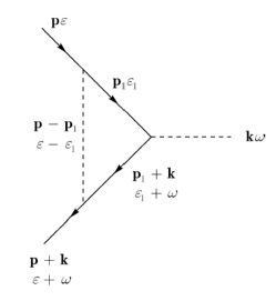
We shall limit our analysis to a model with Einstein spectrum of phonons. The analytic expression corresponding to diagram of Fig. 2 is:

$$\Gamma^{(1)}=-g_{0}^{3}\int G_{0}({\bf p}_{1}\varepsilon_{1})G_{0}({\bf p}_{1}+{\bf k},\varepsilon_{1}+\omega)\times$$

$$\times D_{0}(\varepsilon-\varepsilon_{1},{\bf p-p}_{1})\frac{d^{3}p_{1}d\varepsilon_{1}}{(2\pi)^{4}}$$ (18)

Let us make a rough estimate of this expression. Consider first the integral over $\varepsilon_{1}$. Assuming that the characteristic momentum transfer due to phonon exchange is of the order of $k_{D}\sim p_{F}$, and taking into account that $D_{0}(\varepsilon-\varepsilon_{1})$ drops quadratically in the region of $|\varepsilon-\varepsilon_{1}|\gg\Omega_{0}$, we obtain the main contribution to this integral from the region of $|\varepsilon-\varepsilon_{1}|\sim\Omega_{0}$. Then the integral over $\varepsilon_{1}$ is of the order of 1, and we can write:

$$\Gamma^{(1)}\sim g_{0}^{3}\int d^{3}p_{1}$$

$$\frac{1}{(\varepsilon_{1}-\varepsilon_{\bf p_{1}}+i\delta sign\varepsilon_{\bf p_{1}})(\varepsilon_{1}+\omega-\varepsilon_{\bf p+k}+i\delta sign\varepsilon_{\bf p_{1}+k})}$$

(19)

Consider now the remaining integral over $p_{1}$. Characteristic momentum transfer here is of the order of $k_{D}\sim p_{F}$. Then we can estimate all denominators to be $\sim E_{F}$, and $\int d^{3}p_{1}\sim N(0)E_{F}$. Then we obtain:

$$\Gamma^{(1)}\sim g_{0}^{3}N(0)\frac{E_{F}}{E_{F}^{2}}\sim g_{0}^{3}\frac{N(0)}{\Omega_{0}}\frac{\Omega_{0}}{E_{F}}\sim g_{0}\lambda_{0}\frac{\Omega_{0}}{E_{F}}$$ (20)

Thus the relative size of this correction is:

$$\frac{\Gamma^{(1)}}{g_{0}}\sim\lambda_{0}\frac{\Omega_{0}}{E_{F}}\sim\lambda_{0}\sqrt{\frac{m}{M}}$$ (21)

where we have used $\frac{\Omega_{0}}{E_{F}}\sim\frac{\omega_{D}}{E_{F}}\sim\sqrt{\frac{m}{M}}$, where $m$ is electron mass, $M$ is ion mass. Electrons are much lighter than ions (nuclei) and this correction to vertex part is negligible. More accurate analysis confirms this conclusion AGD ; Scal , which is the essence of Migdal theorem.

Migdal’s theorem allows us to neglect vertex corrections in calculations related to electron – phonon interaction in typical metals. The actual small parameter of perturbation theory is $\lambda_{0}\frac{\Omega_{0}}{E_{F}}\ll 1$, where $\lambda_{0}$ is the dimensionless constant of electron – phonon interaction, $\Omega_{0}$ is characteristic phonon frequency, while $E_{F}$ is Fermi energy of electrons, which in typical metals is of the order of conduction band width and determines the maximal energy scale. In particular this leads to a common belief, that vertex corrections in this theory can be neglected even in case of $\lambda_{0}>1$, until inequality $\frac{\Omega_{0}}{E_{F}}\ll 1$ is valid, which is characteristic for typical metals. In fact this means that taking into account the diagram of Fig. 1 only is sufficient even in the case of strong enough coupling between electrons and phonons.

Previous analysis implicitly assumed conduction band of infinite width. In case of sufficiently large characteristic frequency of phonons it may become comparable not only to Fermi energy, but also to conduction band width. Curiously enough in the limit of very strong nonadiabaticity, when $\Omega_{0}\gg E_{F}\sim D$ ($D$ is conduction band half – width), a new small parameter of perturbation theory $\lambda_{D}/\Omega_{0}\sim\lambda E_{F}/\Omega_{0}$

appears MS_Eli ; MS_Elias . Naturally, $\lambda$ in this case should be calculated using Eq. (17).

Consider the case of conduction band of finite width $2D$ with constant density of states (two – dimensional case). Fermi level as above is assumed to be at zero of energy scale and we assume the typical case of half – filled band, so that $E_{F}=D$. Then Eq. (10) reduces to:

$$\noindent\Sigma(\varepsilon)=\int_{-D}^{D}d\varepsilon^{\prime}\int_{0}^{\infty}d\omega\alpha^{2}(\omega)F(\omega)\Biggl{\{}\frac{f(\varepsilon^{\prime})}{\varepsilon-\varepsilon^{\prime}+\omega-i\delta}+$$

$$+\frac{1-f(\varepsilon^{\prime})}{\varepsilon-\varepsilon^{\prime}-\omega+i\delta}\Biggr{\}}=$$

$$=\int_{0}^{\infty}d\omega\alpha^{2}(\omega)F(\omega)\Biggl{\{}\ln\frac{\varepsilon+D+\omega-i\delta}{\varepsilon-D-\omega+i\delta}$$

$$\noindent-\ln\frac{\varepsilon+\omega-i\delta}{\varepsilon-\omega+i\delta}\Biggr{\}}$$

Correspondingly, from Eq. (III) we get:

$$-\left.\frac{\partial\Sigma(\varepsilon)}{\partial\varepsilon}\right|_{\varepsilon=0}=2\int_{0}^{D}d\varepsilon^{\prime}\int_{0}^{\infty}d\omega\alpha^{2}(\omega)F(\omega)\frac{1}{(\omega+\varepsilon^{\prime})^{2}}$$

$$\noindent=2\int_{0}^{\infty}d\omega\alpha^{2}(\omega)F(\omega)\frac{D}{\omega(\omega+D)}$$

(23)

so that we can define the generalized coupling constant as:

$$\tilde{\lambda}=2\int_{0}^{\infty}\frac{d\omega}{\omega}\alpha^{2}(\omega)F(\omega)\frac{D}{\omega+D}$$ (24)

which for $D\to\infty$ reduces to the usual Eliashberg – McMillan constant (13), while for $D\to 0$ it gives the “antiadiabatic” coupling constant:

$$\lambda_{D}=2D\int\frac{d\omega}{\omega^{2}}\alpha^{2}(\omega)F(\omega)$$ (25)

Eq. (24) describes a smooth crossover between the limits of wide and narrow conduction bands. Mass renormalization, in general, is determined by constant $\tilde{\lambda}$:

$$m^{\star}=m(1+\tilde{\lambda})$$ (26)

For the model of one Einstein phonon with frequency $\Omega_{0}$ we have $F(\omega)=\delta(\omega-\Omega_{0})$, so that:

$$\tilde{\lambda}=\frac{2}{\Omega_{0}}\alpha^{2}(\Omega_{0})\frac{D}{\Omega_{0}+D}=\lambda\frac{D}{\Omega_{0}+D}=\lambda_{D}\frac{\Omega_{0}}{\Omega_{0}+D}$$ (27)

where Eliashberg – McMillan coupling constant:

$$\lambda=2\int_{0}^{\infty}\frac{d\omega}{\omega}\alpha^{2}(\omega)F(\omega)=\alpha^{2}(\Omega_{0})\frac{2}{\Omega_{0}}$$ (28)

Comparison with Eq. (16) gives $\alpha^{2}(\Omega_{0})=g_{0}^{2}N(0)$ and $\lambda_{D}$ reduces to:

$$\lambda_{D}=2\alpha^{2}(\Omega_{0})\frac{D}{\Omega_{0}^{2}}=2\alpha^{2}(\Omega_{0})\frac{1}{\Omega_{0}}\frac{D}{\Omega_{0}}$$ (29)

where in the last term we have explicitly written the new small parameter $D/\Omega_{0}\ll 1$, appearing in the strong antiadiabatic limit. Correspondingly, in this limit we always have:

$$\lambda_{D}=\lambda\frac{D}{\Omega_{0}}\sim\lambda\frac{E_{F}}{\Omega_{0}}\ll\lambda$$ (30)

so that for reasonable values of $\lambda$ (up to the strong coupling region of $\lambda\sim 1$) the “antiadiabatic” coupling constant remains small.

It is obvious that vertex corrections also become small in this limit as was shown by direct calculations in Ref. Ikeda . Thus we came to an unexpected conclusion — in strong antiadiabatic limit electron – phonon coupling becomes weak again! In this sense we can again speak of validity of Migadl theorem also in antiadiabatic limit. The physics here is simple – in strong nonadiabatic limit ions move much faster than electrons, so that electrons can not “adjust” to rapidly changing ion configurations and, in this sense, only are only weakly reacting to ion movements.

IV Strong coupling and lattice instability

The general expression for phonon Green’s function, taking into account the interaction with electrons, is given by Dyson equation shown in Fig. 3.

Figure 3: Dyson equation for the full (“dressed”) phonon Green’s function.

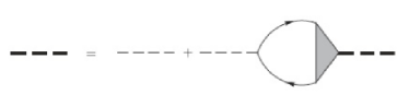
In analytic form we have:

$$D^{-1}({\bf k},i\omega_{m})=D_{0}^{-1}({\bf k},i\omega_{m})-|g_{\bf k}|^{2}\Pi({\bf k},i\omega_{m})$$ (31)

Then we obtain:

$$D({\bf k},i\omega_{m})=\frac{2\Omega_{0{\bf k}}}{(i\omega_{m})^{2}-\Omega_{0{\bf k}}^{2}-2\Omega_{0{\bf k}}|g_{\bf k}|^{2}\Pi({\bf k},i\omega_{m})}$$ (32)

After the usual transition to real frequencies the phonon spectrum (renormalized by interaction) is determined from the equation:

$$\Omega^{2}_{\bf k}=\Omega_{0{\bf k}}^{2}\left[1+\frac{2|g_{\bf k}|^{2}}{\Omega_{0{\bf k}}}\Pi({\bf k},\Omega_{\bf k})\right]$$ (33)

In adiabatic approximation, taking into account Migdal theorem, polarization operator here can be taken as a simple loop. In the simplest case of free electrons we have Diagr :

$$\Pi({\bf k},\omega_{m})=-2N(0)\left\{1+\frac{i\omega_{m}}{2v_{F}k}\ln\frac{i\omega_{m}-v_{F}k}{i\omega_{m}+v_{F}k}\right\}$$ (34)

or, after $i\omega_{m}\to\omega+i\delta$

$$\Pi({\bf k},\omega+i\delta)=-2N(0)\left\{1+\frac{\omega}{2v_{F}k}\ln\frac{\omega-v_{F}k+i\delta}{\omega+v_{F}k+i\delta}\right\}$$ (35)

where $v_{F}$ is electron velocity at Fermi surface, which much exceeds the sound velocity, so that the values of $v_{F}k$ are much higher than frequencies of acoustical phonons, and for typical $k\sim p_{F}$ also those of optical phonons. This again demonstrates the importance of adiabatic approximation in metals. Thus, in calculations of phonon spectrum using (33) we can, with high accuracy, immediately put $\omega=0$ in polarization operator. In this case the imaginary part of polarization operator becomes zero and we simply have $\Pi(0,0)=-2N(0)$. Then the phonon spectrum, renormalized by interaction with electrons, is determined from:

$$\Omega^{2}_{\bf k}=\Omega_{0{\bf k}}^{2}\left[1+\frac{2|g_{\bf k}|^{2}}{\Omega_{0\bf k}}\Pi(0,0)\right]=\Omega_{0\bf k}^{2}\left[1+\frac{\lambda_{0}^{k}}{N(0)}\Pi(0,0)\right]$$ (36)

and takes the form:

$$\Omega^{2}_{\bf k}=\Omega_{0\bf k}^{2}[1-2\lambda_{0}^{k}]$$ (37)

where we have introduced the usual definition of dimensionless coupling constant of electron – phonon interaction Diagr :

$$\lambda_{0}^{k}=\frac{2|g_{\bf k}|^{2}N(0)}{\Omega_{0{\bf k}}}$$ (38)

In this (rough enough) approximation the relatively small damping of phonons due to electron – phonon interaction just vanishes. It can be obtained with more accurate treatment of the imaginary part of polarization operator Diagr .

The “bare” Green’ function of phonons at real frequencies ($T=0$)

$$D_{0}({\bf k}\omega)=\frac{1}{\omega-\Omega_{0{\bf k}}+i\delta}-\frac{1}{\omega+\Omega_{0{\bf k}}-i\delta}=\frac{2\Omega_{0{\bf k}}}{\omega^{2}-\Omega^{2}_{0{\bf k}}+i\delta}$$ (39)

after such “dressing” by interaction with electrons transforms into Diagr :

$$D({\bf k}\omega)=\frac{2\Omega_{0{\bf k}}}{\omega^{2}-\Omega^{2}_{\bf k}+i\delta}$$ (40)

where the renormalized phonon spectrum is given by (37).

The spectrum given by Eq. (37) signifies the lattice instability for $\lambda_{0}^{k}>1/2$. This instability is often considered to be unphysical, as was noted already in an early paper by Fröhlich Frol , where it was obtained for the first time. This point can be explained as follows. Let us rewrite the “dressed” Green’s function (40) identically as:

$$D({\bf k}\omega)=\frac{2\Omega_{\bf k}}{\omega^{2}-\Omega^{2}_{\bf k}+i\delta}\frac{\Omega_{0{\bf k}}}{\Omega_{\bf k}}$$ (41)

Then it becomes clear that during diagram calculations, and Fig. 1 in particular for electron self – energy, using from the very beginning this renormalized Green’s function of phonons, the physical coupling constant of electron – phonon coupling takes the form (instead of (38)):

$$\lambda^{k}=\frac{2|g_{\bf k}|^{2}N(0)}{\Omega_{\bf{k}}}\frac{\Omega_{0{\bf k}}}{\Omega_{\bf k}}=\frac{2|g_{\bf k}|^{2}N(0)}{\Omega_{0{\bf k}}}\frac{\Omega^{2}_{0{\bf k}}}{\Omega^{2}_{\bf k}}=\lambda_{0}^{k}\frac{\Omega^{2}_{\bf k}}{\Omega^{2}_{\bf k}}$$ (42)

or, using (37):

$$\lambda^{k}=\frac{\lambda_{0}^{k}}{1-2\lambda_{0}^{k}}$$ (43)

We see, that for $\lambda_{0}^{k}\to 1/2$ the renormalized coupling constant $\lambda^{k}$ monotonously grows and finally diverges. It is this costant that determines the “true” value of electron – phonon interaction (with “dressed” phonons) and there is no limitations for its value at all. This physical picture was discussed in detail, e.g. in the famous book MaxKh .

In a model with single Einstein phonon, which is a reasonable approximation for an optical phonon, we have $\Omega_{\bf k}=\Omega_{0}$ and we can forget about dependence of the coupling constant on phonon momentum, so that:

$$\lambda_{0}=\frac{2g_{0}^{2}N(0)}{\Omega_{0}}$$ (44)

$$\Omega^{2}=\Omega_{0}^{2}[1-2\lambda_{0}]$$ (45)

$$\lambda=\frac{2g_{0}^{2}N(0)}{\Omega_{0}}\left(\frac{\Omega_{0}}{\Omega}\right)^{2}=\frac{\lambda_{0}}{1-2\lambda_{0}}$$ (46)

Eq. (43) can be reversed and we can write:

$$\lambda_{0}^{k}=\frac{\lambda^{k}}{1+2\lambda^{k}}$$ (47)

expressing nonphysical “bare” constant of electron – phonon coupling $\lambda_{0}^{k}$ via the “true” physical coupling constant $\lambda^{k}$. Using this relation in the equation for renormalized phonon spectrum (37), we can write it as:

$$\Omega^{2}_{\bf k}=\Omega_{0{\bf k}}^{2}\left[1-\frac{2\lambda^{k}}{1+2\lambda^{k}}\right]=\Omega_{0{\bf k}}^{2}\frac{1}{1+2\lambda^{k}}$$ (48)

so that in this representation there is no instability of spectrum (lattice), and the growth of $\lambda^{k}$ just leads to continuous “softening” of spectrum due to the growth of electron – phonon coupling.

In a model of Einstein phonon all relations simplify and we get:

$$\lambda_{0}=\frac{\lambda}{1+2\lambda}$$ (49)

$$\Omega=\frac{\Omega_{0}}{\sqrt{1+2\lambda}}$$ (50)

In Eliashberg – McMillan formalism, where we perform the averaging over the momenta of electrons on the (arbitrary) Fermi surface, McMillan function $\alpha^{2}(\omega)F(\omega)$, naturally should be determined bu the physical (renormalized) spectrum of phonons:

$$\alpha^{2}(\omega)F(\omega)=\frac{1}{N(0)}\sum_{\bf pp^{\prime}}|g_{\bf pp^{\prime}}|^{2}\delta(\omega-\Omega_{\bf p-p^{\prime}})\delta(\varepsilon_{\bf p})\delta(\varepsilon_{\bf p^{\prime}})$$ (51)

In particular case of Einstein phonon it immediately reduces to (46) and there is no limitations on the value of $\lambda$.

In self – consistent derivation of Eliashberg equations we have to use the diagram of Fig. 1, where the the phonon Green’s function is taken in “dressed” form (40) or (41) and describes the physical (renormalized) phonon spectrum. In this case we do not have to include corrections to this function due to electron – phonon interaction, as they are already taken into account in phonon spectrum (37).

It should be noted that the value of critical coupling constant obtained above, at which Fröhlich instability of phonon spectrum appears, is obviously directly related to the use of the simplest expression for polarization operator of the gas of free electrons (34), (35), which was calculated neglecting vertex corrections and self – consistent “dressing” of electron Green’s functions entering the loop. Naturally, even in the simplest cases like the problem with Einstein spectrum accounting for these higher corrections, as well as more realistic structure of electron spectrum in a lattice, can somehow change the value of $\lambda_{0}$, corresponding to instability of the “bare” phonon spectrum, so that it will differ from 1/2. In this sense it is better to speak about instability at some “critical” value $\lambda_{0}^{c}\sim 1/2$.

In general case the inverse influence of electrons on phonons can be taken into account by generalizing Eq. (51) in the following way:

$$\alpha^{2}(\omega)F(\omega)=\frac{1}{N(0)}\sum_{\bf pp^{\prime}}|g_{\bf pp^{\prime}}|^{2}\left(-\frac{1}{\pi}ImD^{R}(\omega,{\bf p-p^{\prime}})\right)$$

$$\times\delta(\varepsilon_{\bf p})\delta(\varepsilon_{\bf p^{\prime}})=$$

$$=\frac{1}{N(0)}\sum_{\bf pp^{\prime}}|g_{\bf pp^{\prime}}|^{2}B({\bf p-p^{\prime}},\omega)\delta(\varepsilon_{\bf p})\delta(\varepsilon_{\bf p^{\prime}})$$ (52)

where we have introduced phonon spectral density $B({\bf q},\omega)$, which determines the phonon Green’s function (in Matsubara representation) via the spectral relation:

$$D({\bf q},i\omega_{m})=\int_{0}^{\infty}B({\bf q},\omega)\frac{2\omega}{(i\omega_{m}^{2})-\omega^{2}}d\omega$$ (53)

In particular, from here we get:

$$D({\bf q},0)=-2\int_{0}^{\infty}\frac{d\omega}{\omega}B({\bf q},\omega)$$ (54)

Then we can write the following general relation for Eliashberg – McMillan constant $\lambda$:

$$\lambda=2\int_{0}^{\infty}\frac{d\omega}{\omega}\alpha^{2}(\omega)F(\omega)=$$

$$=\frac{2}{N(0)}\int_{0}^{\infty}\frac{d\omega}{\omega}\sum_{\bf pp^{\prime}}|g_{\bf pp^{\prime}}|^{2}B({\bf p-p^{\prime}},\omega)\delta(\varepsilon_{\bf p})\delta(\varepsilon_{\bf p^{\prime}})=$$

$$=-\frac{1}{N(0)}\sum_{\bf pp^{\prime}}|g_{\bf pp^{\prime}}|^{2}D({\bf p-p^{\prime}},0)\delta(\varepsilon_{\bf p})\delta(\varepsilon_{\bf p^{\prime}})$$ (55)

For the model of optical phonon with frequency $\Omega_{0}$ this immediately reduces to:

$$\lambda=-g_{0}^{2}N(0)\left\langle D({\bf p-p^{\prime}},0)\right\rangle_{FS}=-\frac{\lambda_{0}\Omega_{0}}{2}\left\langle D({\bf p-p^{\prime}},0)\right\rangle_{FS}$$ (56)

where we have introduced the usual notation for momentum averaging over Fermi surface.

The previous analysis can be significantly improved within simplified Holstein model (3), where the local (single site) nature of interaction allows solving it using the dynamical mean field theory (DMFT) DMFT1 ; DMFT2 ; DMFT3 ; DMFT4 , which becomes (numerically) exact in the limit of lattice of infinite dimensions (infinite number of nearest neighbors). Such analysis was performed e.g. in Ref. Gunn , using as quantum Monte – Carlo (QMC) as impurity solver in DMFT. The main results are shown in Figs. 4, 5.

Figure 4: Dependence of the renormalized coupling constant $\lambda$, calculated from (56), on the “bare” $\lambda_{0}$, obtained within self – consistent Eliashberg theory (ME(RA) – real frequency technique, ME(IA) – Matsubara technique) and in DMFT(QMC) Gunn . Vertical dashed line corresponds to $\lambda_{0}^{c}\approx$0.464.

Figure 5: Dependence of renormalized Einstein phonon frequency $\Omega$ on “bare” $\lambda_{0}$, obtained within self – consistent Eliashberg theory (ME(RA) – real frequency technique, ME(IA) – Matsubara technique) and in DMFT(QMC) Gunn . Vertical dashed line corresponds to $\lambda_{0}^{c}\approx$0.464.

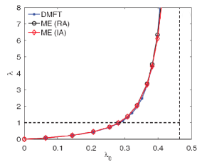
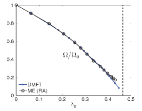
In particular in Fig. 4 we show the dependence of renormalized $\lambda$ on “bare” $\lambda_{0}$. It can be seen, that the usual behavior of Fröhlich theory is nicely reproduced with slightly changed $\lambda_{0}^{c}$=0.464. Similar behavior is observed for renormalized phonon frequency $\Omega$, as seen in Fig. 5. Rather insignificant deviations from predictions of Eliashberg theory are observed only in immediate vicinity of $\lambda_{0}^{c}$, especially for $\lambda_{0}>$0.4.

The instability appearing at $\lambda_{0}=\lambda_{0}^{c}$ in Holstein model (in DMFT approximation) with half – filled bare band, was convincingly interpreted in Ref. Bull as transition into the state of bipolaron insulator. Until this transition the system remains metallic and is nicely described by Eliashberg theory (with insignificant numerical corrections).

In a series of papers Est_1 ; Est_2 ; Est_3 direct calculations by dynamical quantum Monte – Carlo (DQMC) were performed for a number of characteristics of Holstein model on two – dimensional (square) lattice. The results obtained were in some respects similar to the conclusions of Refs. Gunn ; Bull — up to the values of the “bare” constant $\lambda_{0}$=0.4 there is a good agreement with predictions of Eliashberg theory, but in the interval of $\lambda_{0}$ from 0.4 to 0.5 certain deviations are observed. This interval of $\lambda_{0}$ values, according to the same calculations, corresponds to the interval of renormalized $\lambda$ from 1.7 to 4.6. For $\lambda_{0}\approx$ 0.5 system undergoes transition into the state of bipolaron insulator with commensurate charge density wave (CDW).

It is quite clear that the critical value of electron – phonon coupling constant obtained above, corresponding to Fröhlich instability of phonon spectrum at $\lambda_{0}$=1/2, was the direct result of our use of the simplest expression for polarization operator of free electron gas (34), (35), where there was no significant dependence on the wave vector $\bf k$. Naturally, this dependence is also absent in DMFT approximation. If we go to some more realistic model of electron spectrum, like tight – binding approximation in some definite crystal lattice (not in infinite dimensions!), we can obtain instability of phonon spectrum at some finite value of phonon wave vector $\bf k$ Est_1 ; Est_2 ; Est_3 ; Opp . The appearance of such instabilities, as is well known, usually corresponds to formation in the system of charge density waves (CDW) Diagr . In the case of the “nesting” properties of Fermi surface, these instabilities appear (at $T=0$) even for infinitesimal values of the coupling constant of electron – phonon interaction Diagr . After that, metal acquires the new ground state (of dielectric nature) so that all theoretical analysis is to be performed in a new way. In general case, considered here, this instability appears at finite (large enough) values of the “bare” constant of electron – phonon interaction. Naturally, the usual Eliashberg – McMillan theory “works” only within usual metallic phase, which is of the main interest to theory of superconductivity. In this sense, we are in certain disagreement with terminology of Refs. Est_1 ; Est_2 ; Est_3 , where it was claimed, that Eliashberg theory becomes invalid for the values of $\lambda_{0}\sim\lambda_{0}^{c}$. In reality, in this rather narrow region we are observing corrections due to closeness of the system to instability — the phase transition into a new ground state (bipolarons, CDW), where become important fluctuations of corresponding order parameter. Eliashberg theory, considered as a mean – field theory, nicely describes almost all metallic region, except this “critical” neighborhood of $\lambda_{0}^{c}$, including large enough values of physical coupling constant $\lambda$ (which simply diverges at this transition).

It should be stressed here, that all conclusions on instability of metallic phase were done above in the framework of purely model approaches (Fröhlich and Holstein models) and in terms of “bare” parameters of these models like $\lambda_{0}$ and $\Omega_{0}$, which, as was often noted in the literature, are not so well defined physically. This is known for a long time and was discussed many times. The problem nere is that the phonon spectrum in a metal, considered as system of ions and electrons, is usually assumed to be calculated in adiabatic approximation BK . This spectrum is relatively weakly renormalized due to nonadiabatic effects, which are small over the small parameter $\sqrt{\frac{m}{M}}$ BK ; Geilik . In this respect, it is drastically different from the “bare” spectra of Fröhlich or Holstein models, which, as we have seen above, is significantly renormalized by electron – phonon interaction. The physical meaning of the “bare” spectrum $\Omega_{0}$ in these models remains not so clear, in contrast to phonon spectrum in metals, calculated in adiabatic approximation. In any case it can not be determined from any experiments, Similarly, the same can be said about the parameters of electron – phonon interaction. There were numerous attempts to build a consistent theory of electron – phonon interaction on the background of physical (adiabatic) phonon spectrum Geilik , but these were not so successful. Rather detailed discussion of the modern state of this problem can be found in Ref. Maks . The short recipe for practical calculations is to identify the renormalized (“dressed”) spectrum of phonons $\Omega$ in Fröhlich or Holstein models with physical (adiabatic) phonon spectrum, which is not to be further renormalized, and should be taken from adiabatic calculations or from the experiment Precisely this point of view is usually implicitly accepted in calculations within Eliashberg – McMillan theory. Until the system remains in metallic phase, this point of view remains quite consistent. Then there are practically no limitations on the value of physical (renormalized) coupling constant $\lambda$ and Eliashberg – McMillan theory remains valid up to its large enough values (limited only by Migdal theorem).

V McMillan expression for electron – phonon coupling constant

McMillan has derived a simple expression for the dimensionless electron – phonon coupling in Eliashberg theory VIK . Let us write down Eliashberg – McMillan function (8) using (2) as:

$$\alpha^{2}(\omega)F(\omega)=$$

$$=\frac{1}{N(0)}\sum_{\bf p}\sum_{\bf p^{\prime}}|g_{\bf pp^{\prime}}|^{2}\delta(\omega-\Omega_{\bf p-p^{\prime}})\delta(\varepsilon_{\bf p})\delta(\varepsilon_{\bf p^{\prime}})=$$

$$=\frac{1}{N(0)}\sum_{\bf p}\sum_{\bf p^{\prime}}\frac{1}{2M\Omega_{\bf p-p^{\prime}}}|I({\bf p-p^{\prime}})|^{2}\delta(\omega-\Omega_{\bf p-p^{\prime}})$$

$$\times\delta(\varepsilon_{\bf p})\delta(\varepsilon_{\bf p^{\prime}})$$ (57)

where $\Omega_{\bf p-p^{\prime}}$ is assumed to be the physical frequency of phonons. Then we immediately get:

$$\int_{0}^{\infty}d\omega\alpha(\omega)F(\omega)\omega=\frac{N(0)\langle I^{2}\rangle}{2M}$$ (58)

Now rewrite (13)as:

$$\lambda=2\int_{0}^{\infty}\frac{d\omega}{\omega}\alpha^{2}(\omega)F(\omega)=$$

$$=\frac{1}{\langle\Omega^{2}\rangle}\int_{0}^{\infty}d\omega\alpha^{2}(\omega)F(\omega)\omega$$ (59)

where the mean square phonon frequency is defined as:

$$\langle\Omega^{2}\rangle=\frac{\int_{0}^{\infty}d\omega\alpha^{2}(\omega)F(\omega)\omega}{\int_{0}^{\infty}\frac{d\omega}{\omega}\alpha^{2}(\omega)F(\omega)}=$$

$$=\frac{2}{\lambda}\int_{0}^{\infty}d\omega\alpha^{2}(\omega)F(\omega)\omega$$

(60)

From this expression we can immediately see that:

$$\lambda=\frac{N(0)\langle I^{2}\rangle}{M\langle\Omega^{2}\rangle}$$ (61)

where we have introduces the matrix element of the gradient of electron – ion potential averaged over Fermi surface:

$$\langle I^{2}\rangle=\frac{1}{[N(0)]^{2}}\sum_{\bf p}\sum_{\bf p^{\prime}}\left|I({\bf p-p^{\prime}})\right|^{2}\delta(\varepsilon_{\bf p})\delta(\varepsilon_{\bf p^{\prime}})=$$

$$=\frac{1}{[N(0)]^{2}}\sum_{\bf p}\sum_{\bf p^{\prime}}\left|\langle{\bf p}|\nabla V_{ei}({\bf r})|{\bf p^{\prime}}\rangle\right|^{2})\delta(\varepsilon_{\bf p})\delta(\varepsilon_{\bf p^{\prime}})=$$

$$=\langle|\langle{\bf p}|\nabla V_{ei}({\bf r})|{\bf p^{\prime}}\rangle|^{2}\rangle_{FS}$$ (62)

Eq. (61) gives very useful representation for $\lambda$, which is often used in the literature and in practical calculations.

VI Eliashberg equations

Eliashberg theory is based on a system of equations for normal and anomalous Green’s functions of a superconductor Diagr . Obviously, the solution of these integral equations, taking into account the real spectrum of phonons, represents rather difficult problem. However, a significant progress was achieved and the theory of traditional superconductors, based on the picture of pairing due to electron – phonon interaction, is an example of very successful application of Green’s functions. Very good presentation of methods used and applications of Eliashberg equations can be found in Ref. VIK .

Below we shall present somehow simplified derivation of Eliashberg equations, dropping some technical details. In particular, we shall not consider the role of direct Coulomb repulsion of electrons within Cooper pair, which is accounted for in the complete Eliashberg – McMillan theory VIK , limiting ourselves only to electron – phonon interaction. The accounting for Coulomb contributions is not especially difficult VIK and reduces at the end to introduction of Coulomb pseudopotential $\mu^{\star}$ VIK , which in typical metals is rather small and not so important in the limit of very strong coupling with phonons, which will be of the main interest for us in the following

Taking into account Migdal theorem, in adiabatic approximation vertex corrections are irrelevant, so that Eliashberg equations can be derived by calculating the diagram of Fig. 1, where electron Green’s function in superconducting state is taken in Nambu matrix representation Schr . Calculations are similar to derivation of (10) and can be performed in Matsubara technique ($T\neq 0$). In Nambu formalism electronic Green’s function of superconductor is written in a standard way as ($\hat{\sigma}_{i}$ are Pauli matrices) VIK :

$$\hat{G}^{-1}(i\omega_{n},{\bf p})=i\omega_{n}\hat{1}-\varepsilon_{\bf p}\hat{\sigma}_{z}-\hat{\Sigma}(i\omega_{n},{\bf p})$$ (63)

where matrix self – energy is represented as:

$$\hat{\Sigma}(i\omega_{n},{\bf p})=(1-Z(i\omega_{n}))i\omega_{n}\hat{1}+Z(i\omega_{n})\Delta(i\omega_{n})\hat{\sigma}_{x}$$ (64)

Here we are introducing a number of simplifying assumptions like independence of renormalization factor $Z(i\omega_{n})$ and gap function $\Delta(i\omega_{n})$ on momentum VIK . Then we have:

$$\hat{G}(i\omega_{n},{\bf p})=\frac{Z(i\omega_{n})i\omega_{n}\hat{1}+\varepsilon_{\bf p}\hat{\sigma}_{z}+Z(i\omega_{n})\Delta(i\omega_{n})\hat{\sigma}_{x}}{Z^{2}(i\omega_{n})(i\omega_{n})^{2}-Z^{2}(i\omega_{n})\Delta^{2}(i\omega_{n})-\varepsilon^{2}_{\bf p}}$$ (65)

Self – energy part corresponding to diagram like Fig. 1 with matrix Green’s function of electron (65) is written as:

$$\hat{\Sigma}(\omega_{n},{\bf p})=-T\sum_{m}\sum_{\bf p^{\prime}}|g_{\bf pp^{\prime}}|^{2}D(i\omega_{n}-i\omega_{m},{\bf p-p^{\prime}})\times$$

$$\times\hat{\sigma}_{z}\hat{G}({i\omega_{m},\bf p^{\prime}})\hat{\sigma}_{z}$$ (66)

where phonon Green’s function $D(i\omega_{n}-i\omega_{m},{\bf p-p^{\prime}})$ can be taken as in Eq. (39), denoting the phonon frequency $\Omega_{\bf p-p^{\prime}}$ as in Eq. (6).

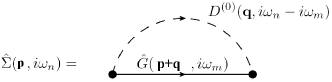
As we know, all physics of conventional superconductivity develops in a layer with the width of the order of $2\Omega_{D}\ll E_{F}$ close to Fermi surface. Thus we can make here the substitution (8) and obtain from (66) the expression for self – energy part averaged over momenta on Fermi surface (similar to (10)). As a result, we obtain the general system of equations for the gap $\Delta(\omega_{n})$ and renormalization factor $Z(\omega_{n})$ of the following form:

$$\Delta(\omega_{n})Z(\omega_{n})=T\sum_{n^{\prime}}\int_{-\infty}^{\infty}d\xi\int_{0}^{\infty}d\omega\alpha^{2}(\omega)F(\omega)\times$$

$$\times D(\omega_{n}-\omega_{n^{\prime}};\omega)\frac{\Delta(\omega_{n}^{\prime})}{\omega^{2}{{}_{n}^{\prime}}+\xi^{2}+\Delta^{2}(\omega_{n^{\prime}})}$$ (67)

$$1-Z(\omega_{n})=\frac{\pi T}{\omega_{n}}\sum_{n^{\prime}}\int_{-\infty}^{\infty}d\xi\int_{0}^{\infty}d\omega\alpha^{2}(\omega)F(\omega)\times$$

$$\times D(\omega_{n}-\omega_{n^{\prime}};\omega)\frac{\omega_{n}^{\prime}}{\omega^{2}{{}_{n}^{\prime}}+\xi^{2}+\Delta^{2}(\omega_{n^{\prime}})}$$ (68)

where we have introduced

$$D(\omega_{n}-\omega_{n^{\prime}};\omega)=\frac{2\omega}{(\omega_{n}-\omega_{n^{\prime}})^{2}+\omega^{2}}$$ (69)

The integral over $\xi$ here is easily calculated and gives:

$$\int_{-\infty}^{\infty}d\xi\frac{1}{\omega_{n^{\prime}}^{2}+\xi^{2}+\Delta^{2}(\omega_{n^{\prime}})}=\frac{\pi}{\sqrt{\omega_{n^{\prime}}^{2}+\Delta^{2}(\omega_{n^{\prime}})}}\to$$

$$\to\frac{\pi}{|\omega_{n^{\prime}}|}\ \mbox{for}\ \Delta(\omega_{n^{\prime}})\to 0$$ (70)

Then the linearized gap equation (equation for $T_{c}$) has the form:

$$\Delta(\omega_{n})Z(\omega_{n})=\pi T\sum_{n^{\prime}}\int_{0}^{\infty}\alpha^{2}(\omega)F(\omega)\times$$

$$\times D(\omega_{n}-\omega_{n^{\prime}};\omega)\frac{\Delta(\omega_{n^{\prime}})}{|\omega_{n^{\prime}}|}$$ (71)

where

$$1-Z(\omega_{n})=\frac{\pi T}{\omega_{n}}\sum_{n^{\prime}}\int_{-\infty}^{\infty}d\xi\int_{0}^{\infty}d\omega\alpha^{2}(\omega)F(\omega)\times$$

$$\times D(\omega_{n}-\omega_{n^{\prime}};\omega)\frac{\omega_{n^{\prime}}}{|\omega{{}_{n}^{\prime}}|}$$ (72)

The general gap equation is:

$$\Delta(\omega_{n})Z(\omega_{n})=\pi T\sum_{n^{\prime}}\int_{0}^{\infty}\alpha^{2}(\omega)F(\omega)\times$$

$$\times D(\omega_{n}-\omega_{n^{\prime}};\omega)\frac{\Delta(\omega_{n^{\prime}})}{\sqrt{\omega^{2}_{n^{\prime}}+\Delta^{2}(\omega_{n^{\prime}})}}$$ (73)

where factor $Z(\omega_{n})$ is determined from the following equation:

$$1-Z(\omega_{n})=\frac{\pi T}{\omega_{n}}\sum_{n^{\prime}}\int_{0}^{\infty}d\omega\alpha^{2}(\omega)F(\omega)\times$$

$$\times D(\omega_{n}-\omega_{n^{\prime}};\omega)\frac{\omega_{n^{\prime}}}{\sqrt{\omega_{n^{\prime}}^{2}+\Delta^{2}(\omega_{n^{\prime}})}}$$ (74)

to be solved jointly with (73).

In a model with Einstein spectrum of phonons Eq. (73) reduces to:

$$\Delta(\omega_{n})Z(\omega_{n})=\pi T\lambda\sum_{n^{\prime}}\frac{\Omega_{0}^{2}}{(\omega_{n}-\omega_{n^{\prime}})^{2}+\Omega_{0}^{2}}\times$$

$$\times\frac{\Delta(\omega_{n^{\prime}})}{\sqrt{\omega^{2}_{n^{\prime}}+\Delta^{2}(\omega_{n^{\prime}})}}$$ (75)

while Eq. (74) becomes:

$$Z(\omega_{n})=1+\frac{\pi T\lambda}{\omega_{n}}\sum_{n^{\prime}}\frac{\Omega_{0}^{2}}{(\omega_{n}-\omega_{n^{\prime}})^{2}+\Omega_{0}^{2}}\frac{\omega_{n^{\prime}}}{\sqrt{\omega_{n^{\prime}}^{2}+\Delta^{2}(\omega_{n^{\prime}})}}$$ (76)

where the coupling constant $\lambda$, determined by standard expressions (13) or (28), appears explicitly.

To determine $T_{c}$ (in the limit of $\Delta(\omega_{n^{\prime}})\to 0$) in a system with Einstein spectrum of phonons we obtain the following system of linear homogeneous Eliashberg equations:

$$\Delta(\omega_{n})Z(\omega_{n})=\pi T\lambda\sum_{n^{\prime}}\frac{\Omega^{2}_{0}}{(\omega_{n}-\omega_{n^{\prime}})^{2}+\Omega_{0}^{2}}\frac{\Delta(\omega_{n^{\prime}})}{|\omega_{n^{\prime}}|}$$ (77)

where

$$Z(\omega_{n})=1+\frac{\pi T\lambda}{\omega_{n}}\sum_{n^{\prime}}\frac{\Omega_{0}^{2}}{(\omega_{n}-\omega_{n^{\prime}})^{2}+\Omega_{0}^{2}}\frac{\omega_{n^{\prime}}}{|\omega_{n^{\prime}}|}$$ (78)

It is clear that the value of $T_{c}$ is determined by zero determinant of this system of equations.

Note that in general equations (73), (74) the coupling constant $\lambda$ does not appear explicitly. Usually this is achieved by reduction of these equations to “Einstein” form like (75), (76) by introduction of the average square of phonon frequency, defined as:

$$\langle\Omega^{2}\rangle=\frac{2}{\lambda}\int_{0}^{\infty}d\omega\alpha^{2}(\omega)F(\omega)\omega$$ (79)

and the following replacement in (73), (74):

$$\frac{1}{(\omega_{n}-\omega_{n^{\prime}})^{2}+\omega^{2}}\Longrightarrow\frac{1}{(\omega_{n}-\omega_{n^{\prime}})^{2}+\langle\Omega^{2}\rangle}$$ (80)

which gives (75), (76), and also the equations for $T_{c}$ (77), (78) with simple replacement of $\Omega^{2}_{0}$ by $\langle\Omega^{2}\rangle$. In this sense the general structure “Einstein” Eliashberg equations conserves also for the case of general phonon spectrum. This approximation with identification of $\Omega^{2}_{0}$ and $\langle\Omega^{2}\rangle$ is always assumed in the following.

For the model of phonon spectrum consisting of discreet set of Einstein phonons:

$$\alpha^{2}(\omega)F(\omega)=\sum_{i}\alpha^{2}(\Omega_{i})\delta(\omega-\Omega_{i})$$

$$=\sum_{i}\frac{\lambda_{i}}{2}\Omega_{i}\delta(\omega-\Omega_{i})$$ (81)

In this case from (79) we simply obtain:

$$\langle\Omega^{2}\rangle=\frac{1}{\lambda}\sum_{i}\lambda_{i}\Omega_{i}^{2}$$ (82)

where $\lambda=\sum_{i}\lambda_{i}$.

VI.1 Weak and intermediate coupling

There is a vast literature on solving Eliashberg equations in the weak or intermediate coupling region $\lambda<$1 Scal ; All ; VIK . Here we only present qualitative results for $T_{c}$, dropping unimportant (for our aims) numerical coefficients $\sim$1. In a model with Einstein spectrum of phonons and Coulomb potential $\mu^{\star}$=0 we have Diagr :

$$T_{c}\sim\Omega_{0}\exp\left(-\frac{1+\lambda}{\lambda}\right)$$ (83)

This expression is in fact close to the results of an exact numerical analysis performed at a time by McMillan Scal ; All ; VIK

Similar estimates of $T_{c}$ can be obtained also in the strong antiadiabatic limit, considering Eliashberg equations for $\lambda<$1 in the problem with a narrow electron band of half – width $D\sim E_{F}\ll\Omega_{0}$ MS_Eli ; MS_Elis ; MS_Elias . Then the appropriately generalized Eliashberg equations give for the same model with Einstein spectrum:

$$T_{c}\sim\frac{D}{1+D/\Omega_{0}}\exp\left(-\frac{1+\tilde{\lambda}}{\lambda}\right)$$ (84)

where the effective constant $\tilde{\lambda}$ was defined above in Eqs. (24), (27) and (30).

Eq. (84) interpolates between adiabatic and antiadiabatic limits. For $D\gg\Omega_{0}$ it gives (83), while for $D\ll\Omega_{0}$ it reduces to:

$$T_{c}\sim D\exp\left(-\frac{1}{\lambda}\right)$$ (85)

i.e. to BCS – like expression (weak coupling!), where preexponential factor is determined not by phonon frequency, but by the electron band half – width (Fermi energy), which now plays the role of cutoff parameter for divergence in Cooper channel. This fact was first noted by Gor’kov in Refs. Gork_1 ; Gork_2 ; Gork_3 .

For more general model of phonon spectrum consisting of discrete set of Einstein phonons (81) these relations are obviously generalized to MS_Elis ; MS_Elias :

$$\lambda=2\sum_{i}\frac{\alpha^{2}(\Omega_{i})}{\Omega_{i}}\equiv\sum_{i}\lambda_{i}$$ (86)

$$\tilde{\lambda}=2\sum_{i}\frac{\alpha^{2}(\Omega_{i})D}{\Omega_{i}(\Omega_{i}+D)}=\sum_{i}\lambda_{i}\frac{D}{\Omega_{i}+D}\equiv\sum_{i}\tilde{\lambda}_{i}$$ (87)

and instead of (84) we have:

$$T_{c}\sim\prod_{i}\left(\frac{D}{1+\frac{D}{\Omega_{i}}}\right)^{\frac{\lambda_{i}}{\lambda}}\exp\left(-\frac{1+\tilde{\lambda}}{\lambda}\right)$$ (88)

In the simplest case of two Einstein phonons with frequencies $\Omega_{1}$ and $\Omega_{2}$ this gives:

$$T_{c}\sim\left(\frac{D}{1+\frac{D}{\Omega_{1}}}\right)^{\frac{\lambda_{1}}{\lambda}}\left(\frac{D}{1+\frac{D}{\Omega_{2}}}\right)^{\frac{\lambda_{2}}{\lambda}}\exp\left(-\frac{1+\tilde{\lambda}}{\lambda}\right)$$ (89)

where $\tilde{\lambda}=\tilde{\lambda}_{1}+\tilde{\lambda}_{2}$ and $\lambda=\lambda_{1}+\lambda_{2}$. In case of $\Omega_{1}\ll D$ (adiabatic phonon), and $\Omega_{2}\gg D$ (antiadiabatic phonon) (89) reduces to:

$$T_{c}\sim(\Omega_{1})^{\frac{\lambda_{1}}{\lambda}}(D)^{\frac{\lambda_{2}}{\lambda}}\exp\left(-\frac{1+\tilde{\lambda}}{\lambda}\right)$$ (90)

Eq. (88) is easily rewritten as:

$$T_{c}\sim\langle\Omega_{\ln}\rangle\exp\left(-\frac{1+\tilde{\lambda}}{\lambda}\right)$$ (91)

where we have introduced mean logarithmic frequency $\langle\Omega_{\ln}\rangle$:

$$\ln\langle\Omega_{\ln}\rangle=\ln\prod_{i}\left(\frac{D}{1+\frac{D}{\Omega_{i}}}\right)^{\frac{\lambda_{i}}{\lambda}}=\sum_{i}\frac{\lambda_{i}}{\lambda}\ln\frac{D}{1+\frac{D}{\Omega_{i}}}$$ (92)

In the limit of continuous distribution of phonon frequencies the last expression reduces to:

$$\ln\langle\Omega_{\ln}\rangle=\frac{2}{\lambda}\int\frac{d\omega}{\omega}\alpha^{2}(\omega)F(\omega)\ln\frac{D}{1+\frac{D}{\omega}}$$ (93)

where $\lambda$ is given by the usual relation (13).

In general case, the preexponential factor in the expression for $T_{c}$ in Eliashberg theory for weak or intermediate coupling is always given by mean logarithmic phonon frequency VIK , and Eq. (93) gives the generalization of the standard expression for this frequency for the case of electron band of finite width. From Eq. (93) we can easily obtain the standard expression VIK (see also below) for adiabatic limit, when $D\to\infty$.

VI.2 Lower bound for $T_{c}$ in the limit of very strong coupling

To achieve really high values of $T_{c}$ the region of strong and very strong coupling $\lambda>1$ is of the main interest and will be discussed in the following. The general Eliashberg equations in Matsubara representation, determining superconducting gap $\Delta(\omega_{n})$ at arbitrary temperatures, are given in (73), (74) Scal ; All .

Limitations on the value of $T_{c}$ in the limit of very strong coupling are easily derived analytically. We shall see shortly, that appropriate behavior follows form the estimate of the lower bound for $T_{c}$ AD . Consider the linearized gap equation (71), determining $T_{c}$:

$$\Delta(\omega_{n})Z(\omega_{n})=\pi T\sum_{n^{\prime}}\int_{0}^{\infty}\alpha^{2}(\omega)F(\omega)\times$$

$$\times D(\omega_{n}-\omega_{n^{\prime}};\omega)\frac{\Delta(\omega_{n^{\prime}})}{|\omega_{n^{\prime}}|}$$ (94)

where phonon Green’s function is defined in (69). Let us consider the term with $n=0$. Then, leaving in the sum in Eq. (78) only the contribution from $n^{\prime}=0$, we obtain:

$$Z(0)=1+\lambda$$ (95)

which after the substitution into Eq. (94) for $n=0$ just cancels the similar (corresponding to $n^{\prime}=0$) term in the r.h.s. of Eq. Kres ; Kresin_Gut , so that the equation for $\Delta(0)=\Delta(\pi T)$ takes the form:

$$\Delta(0)=\pi T\sum_{n^{\prime}\neq 0}\int_{0}^{\infty}\alpha^{2}(\omega)F(\omega)\frac{2\omega}{(\pi T-\omega_{n^{\prime}})^{2}+\omega^{2}}\frac{\Delta(\omega_{n^{\prime}})}{|\omega_{n^{\prime}}|}$$ (96)

All terms in the r.h.s. here are positive. Let us leave only the contribution from $n^{\prime}=-1$, so that taking into account $\Delta(-1)=\Delta(-\pi T)=\Delta(\pi T)=\Delta(0)$, and canceling $\Delta(0)$ in l.h.s and r.h.s. we immediately get the inequality AD :

$$1>\int_{0}^{\infty}d\omega\frac{2\alpha^{2}(\omega)F(\omega)\omega}{(2\pi T)^{2}+\omega^{2}}$$ (97)

Actually here $T=T_{c}$, and this equation gives the lower estimate of $T_{c}$. In particular, in the model with Einstein spectrum of phonons $F(\omega)=\delta(\omega-\Omega_{0})$ and this inequality is immediately rewritten as:

$$1>2\alpha^{2}(\Omega_{0})\frac{\Omega_{0}}{(2\pi T)^{2}+\Omega_{0}^{2}}=\lambda\frac{\Omega^{2}_{0}}{(2\pi T)^{2}+\Omega_{0}^{2}}$$ (98)

so that for $T_{c}$ we get:

$$T_{c}>\frac{1}{2\pi}\sqrt{\lambda-1}\Omega_{0}$$ (99)

which for $\lambda\gg 1$ reduces to:

$$T_{c}>\frac{1}{2\pi}\sqrt{\lambda}\Omega_{0}\approx 0.16\sqrt{\lambda}\Omega_{0}$$ (100)

Figure 6: Temperature of superconducting transition in Einstein model of phonon spectrum in units of $T_{c}/\Omega_{0}$ as a function of pairing constant $\lambda$ AD : 1 – lower bound (99), 2 – solution of the system of two linear equations ($n=0,\pm 1$), 3 – numerically exact solution of the full system of equations ($n\leq 63$) AD . McMillan expression for $T_{c}$ VIK is shown by dashed line (for the case of $\mu^{\star}$=0).

For discrete spectrum of phonons (81) inequality (97) reduces to:

$$1>\sum_{i}\lambda_{i}\frac{\Omega_{i}^{2}}{(2\pi T)^{2}+\Omega_{i}^{2}}$$ (101)

which in the limit of very strong coupling for $2\pi T\gg\Omega_{i}$ immediately gives the natural generalization of (100):

$$T_{c}>\frac{1}{2\pi}\sqrt{\lambda\langle\Omega^{2}\rangle}$$ (102)

where $\lambda=\sum_{i}\lambda_{i}$ and $\langle\Omega^{2}\rangle$ was defined above in Eq. (82).

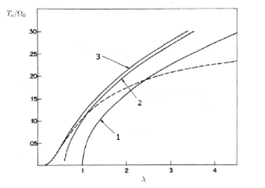
If we solve 2$\times$2 system of equations and appropriate quadratic equation for $T_{c}$, following from Eqs. (77), (78) for $n=0;\pm 1$, the constant 0.16 in (100) is replaced by 0.18. The solution of system with $n\leq$63, performed in Ref. AD lead to replacement of 0.18 by 0.182, which practically corresponds to numerically exact solution. It is obvious, that even the simplest solution (99) is quite sufficient for qualitative estimates of $T_{c}$ in the limit of very strong coupling. The general situation is illustrated in Fig. 6. From this figure it can be seen, in particular, that asymptotic behavior of $T_{c}$ for $\lambda\gg$1 (100) with coefficient 0.18, rather well approximates the values of critical temperature already starting from the values of $\lambda>$1.5-2.0 (cf. curve 2 in this figure).

Consider now the very strong coupling case in strong antiadiabatic limit, though realization of such coupling in this limit is rather doubtful, as pairing constant $\lambda$, defined according to (17), typically rapidly drops with the growth of phonon frequency, as it exceeds Fermi energy MS_Eli ; MS_Elias .

Consider again the electron band of finite width $2D$ (constant density of states). Then in general Eliashberg equations considered above, instead of integral in infinite limits (70) we have:

$$\int_{-D}^{D}d\xi\frac{1}{\omega_{n^{\prime}}^{2}+\xi^{2}+\Delta^{2}(\omega_{n^{\prime}})}=$$

$$=\frac{2}{\sqrt{\omega_{n^{\prime}}^{2}+\Delta^{2}(\omega_{n^{\prime}})}}arctg\frac{D}{\sqrt{\omega_{n^{\prime}}^{2}+\Delta^{2}(\omega_{n^{\prime}})}}\to$$

$$\to\frac{2}{|\omega_{n^{\prime}}|}arctg\frac{D}{|\omega_{n^{\prime}}|}\ \mbox{for}\ \Delta(\omega_{n^{\prime}})\to 0$$ (103)

Then the linearized Eliashberg equations take the following general form:

$$\Delta(\omega_{n})Z(\omega_{n})=$$

$$=T\sum_{n^{\prime}}\int_{0}^{\infty}d\omega\alpha^{2}(\omega)F(\omega)D(\omega_{n}-\omega_{n^{\prime}};\omega)\times$$

$$\times\frac{2\Delta(\omega_{n^{\prime}})}{|\omega_{n^{\prime}}|}arctg\frac{D}{|\omega_{n^{\prime}}|}$$ (104)

where

$$Z(\omega_{n})=1+\frac{T}{\omega_{n}}\sum_{n^{\prime}}\int_{0}^{\infty}d\omega\alpha^{2}(\omega)F(\omega)\times$$

$$\times D(\omega_{n}-\omega_{n^{\prime}};\omega)\frac{\omega_{n^{\prime}}}{|\omega_{n^{\prime}}|}arctg\frac{D}{|\omega_{n^{\prime}}|}$$ (105)

Now we directly obtain the equation for $\Delta(0)$:

$$\Delta(0)=T\sum_{n^{\prime}\neq 0}\int_{0}^{\infty}d\omega\alpha^{2}(\omega)F(\omega)\frac{2\omega}{(\pi T-\omega_{n^{\prime}})^{2}+\omega^{2}}\times$$

$$\times\frac{2\Delta(\omega_{n^{\prime}})}{|\omega_{n^{\prime}}|}arctg\frac{D}{|\omega_{n^{\prime}}|}$$ (106)

Again, taking into account only the contribution of $n^{\prime}=-1$ in the r.h.s., we immediately obtain an inequality:

$$1>\frac{2}{\pi}\int_{0}^{\infty}d\omega\alpha^{2}(\omega)F(\omega)\frac{2\omega}{(2\pi T)^{2}+\omega^{2}}arctg\frac{D}{\pi T}$$ (107)

In Einstein model of phonon spectrum we have $F(\omega)=\delta(\omega-\Omega_{0})$, so that Eq. (107) reduces to:

$$1>\frac{2}{\pi}\lambda arctg\frac{D}{\pi T}\frac{\Omega^{2}_{0}}{(2\pi T)^{2}+\Omega^{2}_{0}}$$ (108)

For $D\gg\pi T$ it immediately gives the result of Allen and Dynes:

$$T_{c}>\frac{1}{2\pi}\sqrt{\lambda-1}\Omega_{0}\to 0.16\sqrt{\lambda}\Omega_{0}\ \mbox{for}\ \lambda\gg 1\$$ (109)

For $D\ll\pi T$ Eq. (108) gives:

$$T>\frac{1}{2\pi}\sqrt{\lambda^{*}(T)-1}\Omega_{0}$$ (110)

where

$$\lambda^{*}(T)=\frac{2D}{\pi^{2}T}\lambda$$ (111)

so that in strong antiadiabatic limit we have:

$$T_{c}>(2\pi^{4})^{-1/3}(\lambda D\Omega_{0}^{2})^{1/3}\approx 0.17(\lambda D\Omega_{0}^{2})^{1/3}$$ (112)

From the obvious condition $\lambda^{*}(T)>0$ we get:

$$T_{c}<\frac{2}{\pi^{2}}\lambda D\approx 0.202\lambda D$$ (113)

which bounds $T_{c}$ from above.

Figure 7: Temperature of superconducting transition (lower bound) in Einstein model of phonon spectrum in units of $2\pi T_{c}/\Omega_{0}$, as a function of pairing constant $\lambda$ for different values of inverse adiabaticity parameter $D/\Omega_{0}$. Dashed lines show appropriate dependencies for $2\pi T_{c}/\Omega_{0}$ in the region of weak and intermediate coupling (84). Black dashed line — Allen – Dynes estimate (99), valid in adiabatic limit AD

.

Figure 8: Temperature of superconducting transition (lower bound) in Einstein model of phonon spectrum in units of $2\pi T_{c}/D$, as a function of pairing constant $\lambda$ for different values of adiabaticity parameter $\Omega_{0}/D$. Dashed lines show appropriate dependencies for $2\pi T_{c}/D$ in weak and intermediate coupling region (84).

Thus we have to satisfy an inequality:

$$(2\pi^{4})^{-1/3}(\lambda D\Omega_{0}^{2})^{1/3}<T_{c}<\frac{2}{\pi^{2}}\lambda D$$ (114)

which reduces to the condition:

$$\Omega_{0}<\frac{4}{\pi}\lambda D\approx 1.27\lambda D\ \mbox{or}\ \frac{D}{\Omega_{0}}>\frac{0.78}{\lambda}$$ (115)

so that for self – consistency of our analysis we have to satisfy the condition:

$$\lambda\gg\frac{\Omega_{0}}{D}\gg 1$$ (116)

where the last equality corresponds to the limit of strong antiadiabaticity. Correspondingly, all the previous estimates become invalid for $\lambda\sim 1$ and can describe only the limit of very strong coupling.

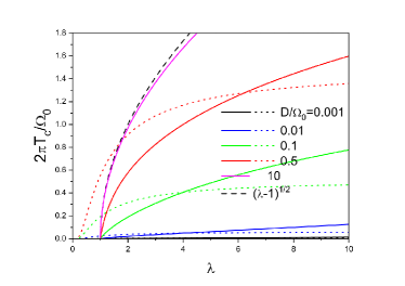
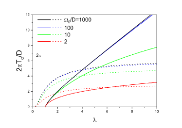
In Fig. 7 and Fig. 8 we show the results of numerical calculations of $T_{c}$ boundaries, following from the solution of (108), as compared to the values of $T_{c}$ in the region of weak and intermediate coupling (84), for different values of adiabaticity parameter $\Omega_{0}/D$. It is clear that in the vicinity of crossing dashed and continuous lines in graphs, shown in Fig. 7 and Fig. 8, we actually have a smooth crossover from $T_{c}$ behavior in the region of weak and intermediate coupling to its asymptotic behavior in very strong coupling region of $\lambda\gg 1$. From Fig. 8 it is seen that the boundary (113) is practically achieved in the region of large values of $\lambda$ and $\Omega_{0}/D$. From these figures we can also see that simple rising of phonon frequency and transition to antiadiabatic limit do not lead, in general, to an increase of $T_{c}$ as compared with adiabatic case.

VII Maximal $T_{c}$?

The problem of maximal possible temperature of superconducting transition has arisen immediately after the creation of BCS theory. It was studied in numerous papers with sometimes contradictory results. Among these papers was the notorious paper by Cohen and Anderson CA , where rather elegant arguments were given, seemingly quite convincing, that characteristic scale of $T_{c}$ values due to electron – phonon, or any other similar mechanism, based on exchange of Bose – like excitations in metals, can be of the order of about 10–30 K only. This paper was immediately seriously criticized in Refs. MaxKh ; DMK , with conclusion that in reality there are no such limitations. Even more, the analysis performed in these papers has shown that Ref. CA is just erroneous. However, the point of view expressed in Cohen – Anderson paper became popular in physics community (Anderson himself till the end of his life adhered to the view expressed in Ref. CA ), so that at the time of discovery of high – temperature superconductivity in cuprates (1986 – 1987), almost total belief was that the “usual” electron – phonon mechanism does not allow values of $T_{c}$ higher, that 30-40 K. Because of this after the discovery of superconductivity in cuprates the “great race” has started for new theoretical models and mechanisms of superconductivity, which may explain the high values of $T_{c}$. The problems of superconductivity in cuprates are outside the scope of this work. Most probably, in cuprates really dominates some kind of non – phonon pairing mechanism (due to antiferromagnetic fluctuations). But most important result of discovery of record values of $T_{c}$ in hydrides under high pressures, in our opinion, is the final (and experimental!) rebuttal of the point of view expressed in Ref. CA .

Thus, the problem of maximal value of $T_{c}$, which may be achieved due to electron – phonon mechanism of Cooper pairing is most important as ever. Below we try to discuss this problem once again within standard approach, based on Eliashberg equations, as most successful theory, describing superconductivity in the system of electrons and phonons in metals.

There is a vast literature on numerical solution of Eliashberg equations for different temperatures and different models of phonon spectrum VIK ; All .

A number of analytic expressions for $T_{c}$ were proposed by different authors, to approximate the results of numerical computations. As an example we quote here the popular interpolation formula for $T_{c}$ due to Allen and Dynes All , which is appropriate for rather wide interval of values of dimensionless coupling constant of electron – phonon interaction $\lambda$, including the strong coupling region of $\lambda>1$:

$$T_{c}=\frac{f_{1}f_{2}}{1.20}\langle\Omega_{\ln}\rangle\exp\left\{-\frac{1.04(1+\lambda)}{\lambda-\mu^{\star}(1+0.62\lambda)}\right\}$$ (117)

where

$$f_{1}=[1+(\lambda/\Lambda_{1})^{3/2}]^{1/3};\ f_{2}=1+\frac{[\langle\Omega^{2}\rangle^{1/2}/\langle\Omega_{\ln}\rangle-1]\lambda^{2}}{\lambda^{2}+\Lambda_{2}^{2}}$$

$$\Lambda_{1}=2.46(1+3.8\mu^{\star});\ \Lambda_{2}=1.82(1+6.3\mu^{\star})\frac{\langle\Omega^{2}\rangle^{1/2}}{\langle\Omega_{\ln}\rangle}$$

(118)

Here $\langle\Omega_{\ln}\rangle$ is the mean logarithmic frequency of phonons:

$$\ln\langle\Omega_{\ln}\rangle=\frac{2}{\lambda}\int_{0}^{\infty}\frac{d\omega}{\omega}\alpha^{2}(\omega)F(\omega)\ln\omega=$$

$$=\frac{\int_{0}^{\infty}\frac{d\omega}{\omega}\ln\omega\alpha^{2}(\omega)F(\omega)}{\int_{0}^{\infty}\frac{d\omega}{\omega}\alpha^{2}(\omega)F(\omega)}$$ (119)

$\langle\Omega^{2}\rangle$ is the average (over the phonon spectrum) square of frequency, defined in Eq. (79):

$$\langle\Omega^{2}\rangle=\frac{2}{\lambda}\int_{0}^{\infty}d\omega\alpha^{2}(\omega)F(\omega)\omega=\frac{\int_{0}^{\infty}d\omega\omega\alpha^{2}(\omega)F(\omega)}{\int_{0}^{\infty}\frac{d\omega}{\omega}\alpha^{2}(\omega)F(\omega)}$$ (120)

The Coulomb pseudopotential $\mu^{\star}$ determines repulsion between electrons within Cooper pair. According to most calculations VIK ; All its values are small and belong to the interval 0.1 – 0.15.

In the limit of very strong coupling $\lambda>10$ this gives the expression for $T_{c}$, which was. in fact. obtained above from simple inequality (99):

$$T_{c}\approx 0.18\sqrt{\lambda\langle\Omega^{2}\rangle}$$ (121)

It may seem now, that limitations on the values of $T_{c}$ are simply absent, so that in the limit of very strong coupling very high $T_{c}$ can be obtained from electron – phonon mechanism. The only more or less obvious limit is related to the limits of adiabatic approximation, which is usually considered to be the cornerstone of Eliashberg theory. However, we have seen above. that similar results can be obtained also in the strong antiadiabatic limit (cf. estimated for $T_{c}$ given in Eqs. (112), (113)).

In the model with Einstein spectrum of phonons we simply have: $\langle\Omega_{\ln}\rangle=\langle\Omega^{2}\rangle^{1/2}=\Omega$, where $\Omega$ is assumed to be the renormalized phonon frequency. Then (121) reduces to:

$$T_{c}=0.18\sqrt{\lambda}\Omega$$ (122)

so that seemingly for $\lambda\gg 1$ we can, in principle, obtain even $T_{c}>\Omega$. However, if we remember the renormalization of phonon spectrum and take into account Eq. (50), we immediately obtain from Eq. (122):

$$T_{c}=0.18\sqrt{\lambda}\Omega=0.18\Omega_{0}\sqrt{\frac{\lambda}{1+2\lambda}}$$ (123)

which in the limit of $\lambda\gg 1$ tends to the value $T_{c}^{max}\approx 0.13\Omega_{0}$, because of significant softening of phonon spectrum. At the same time, as noted above, the physical meaning of “bare” frequency $\Omega_{0}$ in a metal is poorly defined, and in particular it can not be determined from experiments. Correspondingly, the estimate of Eq. (123) somehow hangs in the air.

However, this analysis is valid only under the condition of rigid fixation of all relation between “bare” and “dressed” phonon spectra. If we “forget” about “bare” spectrum of phonons and consider parameters $\Omega$ and $\lambda$ independent, we can obtain from Eq. (122) very high values of $T_{c}$. A certain , though rather artificial model, leading precisely to this kind of behavior was recently introduced in Ref. KivBerg . It considers the interaction of $N$–component electrons with $N\times N$–component system of Einstein phonons in the limit of $N\to\infty$. It was shown that in this model the renormalization of phonon spectrum due to interaction with conduction electrons is suppressed, so that in the limit of very strong coupling with 1$\ll\lambda\ll N$ we always have Allen – Dynes estimate (122) with $\Omega=\Omega_{0}$.

However, the problem her is, that in real situation we never can consider $\Omega$ and $\lambda$ as independent parameters simply because of the general relations (13) and (79), which express $\lambda$ and $\langle\Omega^{2}\rangle$ via integrals of Eliashberg – McMillan function $\alpha^{2}(\omega)F(\omega)$. In fact, we may rewrite the expression for $T_{c}$ in the region of very strong coupling as:

$$T_{c}=0.18\sqrt{\lambda\langle\Omega^{2}\rangle}=0.25\left[\int_{0}^{\infty}d\omega\alpha^{2}(\omega)F(\omega)\omega\right]^{1/2}$$ (124)

in adiabatic case and, correspondingly

$$T_{c}=(2\pi^{4})^{-1/3}(\lambda D\langle\Omega^{2}\rangle)^{1/3}=$$

$$=(2\pi)^{-1/3}\left[2D\int_{0}^{\infty}d\omega\alpha^{2}(\omega)F(\omega)\omega\right]^{1/3}$$ (125)

in antiadiabatic limit. We see, that these expressions for $T_{c}$ are completely determined by integrals of $\alpha^{2}(\omega)F(\omega)$.

In famous Ref. Leav a simple inequality for $T_{c}$ was proposed, limiting its value by the square $A$ under $\alpha^{2}(\omega)F(\omega)$:

$$T_{c}\leq 0.2309\int_{0}^{\infty}d\omega\alpha^{2}(\omega)F(\omega)\equiv 0.2309A$$ (126)

For the case of Einstein spectrum of phonons, taking into account Eq. (28), this inequality can be rewritten as:

$$T_{c}\leq 0.115\lambda\Omega_{0}$$ (127)

This inequality is relatively often used in calculations.

The limitation given by Eq. (113) obtained above in antiadiabatic limit is essentially quite similar to Eq. (127), with replacement $\Omega_{0}\to 2D$, which is quite natural in antiadiabatic limit.

Connection of $\lambda$ and $\langle\Omega^{2}\rangle$ is markedly expressed in McMillan formula (61) for $\lambda$. If we use this expression in (121), we immediately obtain:

$$T_{c}=0.18\sqrt{\frac{N(0)\langle I^{2}\rangle}{M}}$$ (128)

where

$$\langle I^{2}\rangle=\frac{1}{[N(0)]^{2}}\sum_{\bf p}\sum_{\bf p^{\prime}}\left|I({\bf p-p^{\prime}})\right|^{2}\delta(\varepsilon_{\bf p})\delta(\varepsilon_{\bf p^{\prime}})=$$

$$=\frac{1}{[N(0)]^{2}}\sum_{\bf p}\sum_{\bf p^{\prime}}\left|\langle{\bf p}|\nabla V_{ei}({\bf r})|{\bf p^{\prime}}\rangle\right|^{2})\delta(\varepsilon_{\bf p})\delta(\varepsilon_{\bf p^{\prime}})=$$

$$=\langle|\langle{\bf p}|\nabla V_{ei}({\bf r})|{\bf p^{\prime}}\rangle|^{2}\rangle_{FS}$$ (129)

so that both $\lambda$ and $\langle\Omega^{2}\rangle$ just drop out from expression for $T_{c}$, which is expressed now simply via the averaged over Fermi surface matrix element of the gradient of electron – ion potential, ion mass and electron density of states at the Fermi level. This expression is convenient for “first principle” calculations, where it is often used, but it does not contain illustrative physical parameters in terms of which we usually treat $T_{c}$.

Figure 9: Experimental values of the temperature of superconducting transition for conventional superconductors dependence on their Debye temperature $\Theta_{D}$ Kiv .

In Ref. Kiv a new semiempirical limit for $T_{c}$ was proposed for conventional (electron – phonon) semiconductors, which is written in a very simple form:

$$k_{B}T_{c}\leq A_{max}\Theta_{D}=A_{max}\hbar\Omega_{D}$$ (130)

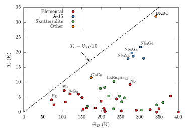
where $A_{max}\approx$ 0.10, and $\Theta_{D}=\hbar\Omega_{D}$ is Debye temperature, which may be determined e.g. from standard measurements of specific heat. This inequality obviously correlated with $T^{max}_{c}$, obtained above in the limit of $\lambda\to\infty$ in Eq. (123), if we identify $\Omega_{0}$ with $\Omega_{D}$. It is seen from Fig. 9 this limitation is satisfied for most of conventional superconductors Kiv . Below we shall see, that is apparently not so in superhydrides.

VIII Superhydrides and Eliashberg theory

In this Section we shall briefly discuss some results of application of Eliashberg theory to $T_{c}$ calculations in hydrides under high pressures. Our presentation here will be very short, much more details may be found, for example, in reviews Grk-Krs ; ErPR ; Ash and in original papers, some of these will be quoted below.

Eliashberg equations were widely used for calculations of $T_{c}$ in hydrides. Actually, both crystal structure of H₃S under high pressures and high values of $T_{c}\sim$200K were predicted in Ref. Duan . For the structure $Im-3m$ under pressure of 200GPa, they obtained the value of pairing constant $\lambda\approx$ 2.2 and mean logarithmic frequency of phonons $\Omega_{ln}\approx$ 1335K, so that for $T_{c}$ calculated from Allen – Dynes expression (117) with Coulomb pseudopotential values $\mu^{\star}=$0.1–0.13 the values of $T_{c}=$191K–204K were obtained. These results were found to be in quite satisfactory agreement with experiment H3S . The achievement of room temperature values of $T_{c}$ in C-S-H system RT was reasonably explained in a recent paper Ge , where it was shown that hole doping of $Im-3m$ structure of H₃S by introduction of carbon shifts Fermi level to a maximum of Van – Hove singularity in the density of states and certain softening of phonon spectrum. Combined, all these lead to the growth of $\lambda$ up to the value of 2.4, which is sufficient, in principle, to explain the values of $T_{c}\approx$288K.

Table 1: Calculated values of $T_{c}$ for La-H and Y-H compounds, obtained from numerical solution of Eliashberg equations Ash compared with its boundary values.

Compound	Pressure (GPa)	$\lambda$	$\Omega_{\ln}$(K)	$T_{c}(\mu^{\star}=0.1)$(K)	$T_{c}$($\mu^{\star}=0.13)$(K)	$\frac{1}{2\pi}\sqrt{\lambda-1}\Omega$	0.18$\sqrt{\lambda}\Omega$
LaH10	210	3.41	848	286	274	209	282
LaH10	250	2.29	1253	274	257	226	341
LaH10	300	1.78	1488	254	241	209	357
YH10	250	2.58	1282	326	305	256	370
YH10	300	2.06	1511	308	286	247	390

In Table 1 we show the calculated parameters of several hydrides of rare – earth elements from Ref. Ash , for which the record values of $T_{c}$ were predicted. In last two columns of the Table we give the boundaries for $T_{c}$, calculated from inequality (99) and from asymptotic expression of Allen and Dynes (122), under the simplest assumption of $\langle\Omega_{\ln}\rangle=\langle\Omega^{2}\rangle^{1/2}=\Omega$. We can see that these values are close enough to those obtained from more detailed calculations of Ref. Ash and determine in fact the lower and upper bounds for $T_{c}$. This clearly shows that the systems with highest values of $T_{c}$ achieved are practically already in the very strong coupling region of Eliashberg theory.

In a recent paper Pick the extensive calculations of $T_{c}$ were performed for practically all possible binary compounds of hydrogen with other elements of periodic system for the values of external pressure 100, 200 and 300 GPa (for which the stable crystal structures were also determined). As many as 36 new systems were discovered for which $T_{c}$ may exceed 100K, and in 18 cases $T_{c}$ exceeded 200K. In particular, for NaH₆ system the values of $T_{c}=$248-279K were obtained, and for CaH₆ — $T_{c}=$216-253K, already for pressured of 100 GPa. The results of this paper clearly show, that the highest possible values of $T_{c}$ are achieved in the region of very strong coupling, up to the values of $\lambda=$5.81 in NaH₆ (under 100 GPa).

Summarizing we may say, that the record values of $T_{c}$ in superhydrides are achieved for typical values of $\lambda=$ 2–3.5 (or even more) and for characteristic phonon frequencies from 1000K to 2000K. We must also note, that the upper bound expressed by Eq. (130) is already quite surpassed in some of the known superhydrides.

IX Conclusions

We consciously presented all problems related to derivation and use of Eliashberg equations on sufficiently elementary level, trying to stress all approximations and simplifications.

Eliashberg theory remains the main theory, which completely explains the values of the critical temperature in superconductors with electron – phonon mechanism of pairing. This theory is also applicable in the region of strong electron – phonon coupling, limited only by the applicability of adiabatic approximation, based on Migdal theorem, which is valid in the vast majority of metals, including the new superhydrides with record values of $T_{c}$. The values of (renormalized, physical) pairing coupling constant $\lambda$ can surely exceed unity until the system possess the metallic ground state. This is not so in the vicinity of phase transition to a new ground state like charge density wave (CDW) or Bose – condensate of bipolarons.

More so, Eliashberg theory is qualitatively applicable also in strong antiadiabatic limit. Simple interpolation expressions for $T_{c}$ can be constructed, connecting adiabatic and antiadiabatic regions, The strong antiadiabatic limit may be of importance in exotic enough systems with very narrow electronic bands and(or) anomalously small values of Fermi energy (like monolayers of FeSe, SrTiO₃ and, probably, some hydrides).

Unfortunately this theory does not produce a simple expression for maximal values of $T_{c}$ in terms of experimentally measurable (or calculated) parameters like characteristic (average) values of phonon frequencies and pairing coupling constant. Formally, such limit is just absent, if we consider these parameters as independent. However, if take into account their interdependence, the maximal values of $T_{c}$ are in fact determined by some “game” of atomic constants. However, all new data on superhydrides strongly indicate that all these systems are very close to the strong coupling region coupling of Eliashberg theory, which means that maximal values of $T_{c}$ for “usual” metals are already achieved. The only hope probably remains only for metallic hydrogen Max .

This work was partially supported by RFBR grant No. 20-02-00011.

References

- (1) A.P. Drozdov, M.I. Eremets, I.A. Troyan, V. Ksenofontov, S.I. Shylin. Nature 525, 73 (2015)
- (2) M.I. Eremets, A.P. Drozdov. Usp. Fiz. Nauk 186, 1257 (2016)
- (3) L.P. Gor’kov, V.Z. Kresin. Rev. Mod. Phys. 90, 01001 (2018)
- (4) C.J. Pickard, I. Errea, M.I. Eremets. Annual Reviews of Condensed Matter Physics 11, 57 (2020)
- (5) J.A. Flores-Livas, L. Boeri, A. Sanna, G. Pinofeta, R. Arita, M. Eremets. Physics Reports 856, 1 (2020)
- (6) H. Liu, I.I. Naumov, R. Hoffman, N.W. Ashcroft, R.J. Hemley. PNAS 114, 6990 (2018)
- (7) A.P. Drozdov, et al. Nature 569, 528 (2019)
- (8) M. Somayazulu, et al. Phys. Rev. Lett. 122, 027001 (2019)
- (9) I.A. Troyan et al. ArXiv:1908.01534; Advanced Materials (2021)
- (10) D.V. Semenok et al. ArXiv:2012.04787; Nature Materials (2021)
- (11) E.Snider, N. Dasenbrock-Gammon, R. McBride, X. Wang, N. Meyers, K.V. Lawler, E. Zurek, A. Salamat, R.P. Dias. Phys. Rev. Lett. 126, 117003 (2021)
- (12) E. Snider, N. Dasenbrock-Gammon, R. McBride, M. Debessai, H. Vindana, K. Vencatasamy, K.V. Lawler, A. Salamat, R.P. Dias. Nature 586, 373 (2020)
- (13) D.J. Scalapino. In “Superconductivity”, p. 449, Ed. by R.D. Parks, Marcel Dekker, NY, 1969
- (14) P.B. Allen, B. Mitrović. Solid State Physics, Vol. Vol. 37 (Eds. F. Seitz, D. Turnbull, H. Ehrenreich), Academic Press, NY, 1982, p. 1
- (15) V.Z. Kresin, H. Morawitz, S.A. Wolf. Superconducting State. Mechanisms and Properties. Oxford University Press, 2014
- (16) S.V. Vonsovsky, Yu. A. Izyumov, E.Z. Kurmaev. Superconductivity of Transition Metals, Their Alloys and Compounds, Springer, Berlin – Heidelberg, 1982
- (17) A.B. Migdal. Zh. Eksp. Teor. Fiz. 34, 1438 (1958) [Sov. Phys. JETP 7, 996 (1958)]
- (18) A.A. Abrikosov, L.P. Gor’kov, I.E. Dzyaloshinskii. Quantum Field Theoretical Methods in Statistical Physics. Pergamon Press, Oxford, 1965
- (19) J.R. Schrieffer. Theory of Superconductivity, WA Benjamin, NY, 1964
- (20) M.V. Sadovskii. Diagrammatics. World Scientific, Singapore, 2019
- (21) I. Esterlis, B. Nosarzewski, E.W. Huang, B. Moritz, T.P. Devereaux, D.J. Scalapino, S.A. Kivelson. Phys. Rev. B97, 140501(R) (2018)
- (22) I. Esterlis, S.A. Kivelson, D.J. Scalapino. Phys. Rev. B99, 174516 (2019)
- (23) A.V. Chubukov, A. Abanov, I. Esterlis, S.A. Kivelson. Ann. Phys. 417, 168190 (2020)
- (24) M.V. Sadovskii. Zh. Eksp. Teor. Fiz. 155, 527 (2019); [JETP 128, 455 (2019)]
- (25) M.V. Sadovskii. Pis’ma J. Esp. Teor. Fiz. 109, 165 (2019) [JETP Letters 109, 166 (2019)]
- (26) M.V. Sadovskii. Journal of Superconductivity and Novel Magnetism 33, 19 (2020)
- (27) M.A. Ikeda, A. Ogasawara, M. Sugihara. Phys. Lett. A 170. 319 (1992)
- (28) M.V. Sadovskii. Usp. Fiz. Nauk 186, 1035 (2016) [Physics Uspekhi 59, 947 (2016)]
- (29) L.P. Gor’kov. Phys. Rev. B93, 054517 (2016)
- (30) L.P. Gor’kov. Phys. Rev. B93, 060507 (2016)
- (31) L.P. Gor’kov. PNAS 113, 4646 (2016)
- (32) Young Woo Choi, Hyong Joon Choi. ArXiv:2103.161132
- (33) H. Fröhlich. Proc. Roy. Soc. A215, 291 (1952)
- (34) High – Temperature Superconductivity. Ed. by V.L. Ginzburg and D.A. Kirzhnits, Consultants Bureau, NY, 1982, Ch. 3
- (35) D. Vollhardt. Correlated Electron Systems (Ed. by V.J. Emery), World Scientific, Singapore, 1993, p. 57
- (36) Th. Pruschke, M. Jarrell, J.K. Freericks. Adv. Phys. 44, 210 (1995)
- (37) A. Georges, G. Kotliar, W. Krauth, M.J. Rozenberg. Rev. Mod. Phys. 68, 13 (1996)
- (38) D. Vollhardt. AIP Conference Proceedings 1297, 339 (2010)
- (39) J. Bauer, J.E. Han, O. Gunnarsson. Phys. Rev. B84, 184531 (2011)
- (40) D. Meyer, A.C. Hewson, R. Bulla. Phys. Rev. Lett. 89, 196401 (2002).
- (41) F. Schrodi, A. Aperis, P.M. Oppeneer. Phys. Rev. B103, 064511 (2021)
- (42) E.G. Brovman, Yu.M. Kagan. Usp. Fiz. Nauk 112, 369 (1974)
- (43) B.T. Geilikman. Usp. Fiz. Nauk 115, 403 (1975)
- (44) E.G. Maksimov, A.E. Karakozov. Usp. Fiz. Nauk 178, 561 (2008)
- (45) P.B. Allen, R.C. Dynes. Phys. Rev. 12, 905 (1975)
- (46) V.Z. Kresin, H. Gutfreund, W.A. Little. Solid State Communications 51, 339 (1984)
- (47) M.L. Cohen, P.W. Anderson. AIP Conference Proceedings on – and – Band Superconductivity, Rochester, NY, 1972, p. 17
- (48) O.V. Dolgov. E.G. Maksimov, D.A. Kirzhnits. Rev. Mod. Phys. 53, 81 (1981)
- (49) J.S. Hoffmann, D. Chowdhuri, S.A. Kivelson, E.Berg. ArXiv:2105.09322
- (50) C.R. Leavens. Solid State Communications 17, 1499 (1975)
- (51) I. Esterlis, S.A. Kivelson, D.J. Scalapino. npj Quant. Mater. 3, 59 (2018)
- (52) D. Duan, Y. Liu, F. Tian, D. Li, X. Huang, Z. Zhao, H. Yu, B. Liu, W. Tian, T. Cui. Sci. Rep. 4, 6968 (2014)
- (53) Y. Ge, F. Zhang, R.P. Dias, R.J. Hemley, Y. Yao. Materials Today Physics 15, 100330 (2020)
- (54) A.M.Shipley, M.J. Hutcheon, R.J. Needs, C.J. Pickard. ArXiv:2105.02296
- (55) E.G. Maksimov. Usp. Fiz. Nauk 178, 175 (2008)