Indicators of Attack Failure: Debugging and Improving Optimization of Adversarial Examples

Abstract

Evaluating robustness of machine-learning models to adversarial examples is a challenging problem. Many defenses have been shown to provide a false sense of security robustness by causing gradient-based attacks to fail, and they have been broken under more rigorous evaluations. Although guidelines and best practices have been suggested to improve current adversarial robustness evaluations, the lack of automatic testing and debugging tools makes it difficult to apply these recommendations in a systematic manner. In this work, we overcome these limitations byproposing: (i) a set of quantitative indicators of failure, which unveil common failures in categorizing attack failures based on how they affect the optimization of gradient-based attacks; and , while also unveiling two novel failures affecting many popular attack implementations and past evaluations; (ii) specific fixes to overcome such failures , which are applied according to a systematic evaluation protocol proposing six novel indicators of failure, to automatically detect the presence of such failures in the attack optimization process; and (iii) suggesting a systematic protocol to apply the corresponding fixes. Our extensive experimental analysis, involving more than 15 models in 3 distinct application domains, shows that our indicators of failure can be used to visualize, debug and improve current adversarial robustness evaluations, thereby providing a first concrete step towards automatizing and systematizing the process of evaluating adversarial robustness of machine-learning modelsthem.

1 Introduction

Despite their unprecedented success in many different applications, machine-learning models have been shown to be vulnerable to adversarial examples [szegedy14-iclr, biggio13-ecml], i.e., inputs intentionally crafted to mislead such models at test time. While hundreds of defenses have been proposed to overcome this issue [xiao19-surv, papernot16-distill, xiao2019resisting, roth2019odds], many of them turned out to only spread a false sense of securitybe ineffective, as their robustness to adversarial inputs was significantly overestimated. In particular, some of them defenses were evaluated by running existing attacks for too few iterations or using inappropriate attack hyperparameters , with inappropriate hyperparameters (e.g., using an insufficient number of iterations), while others were causing implicitly obfuscating gradients, thereby causing the optimization of gradient-based attacks to failby making gradients uninformative or obfuscating them. Such defenses have been indeed shown to yield much lower robustness by running under more rigorous robustness evaluations and adapting attacks using attacks carefully adapted to evade them [carlini17-sp, athalye18].

To prevent the same evaluation mistakesfrom occurring multiple times such evaluation mistakes, and help develop better defenses, several recommendations have been releasedevaluation guidelines and best practices have been described in recent work [carlini2019evaluating]. However, their application is non-trivial, and they have been mostly neglected ; in particular, as their application is non-trivial; in fact, 13 defenses published after the release of these checklists were found to be ineffective due to the difficulty of optimizing the attacks correctlyguidelines were found again to be wrongly evaluated, reporting overestimated adversarial robustness values [tramer2020adaptive]. Moreover, the proposed checklists can themselves provide a false sense of security [popovicgradient], as their application is insufficient to ensure evaluation correctness. While It has also been shown that, even when following such guidelines, robustness can still be overestimated [popovicgradient]. Finally, while recently-proposed evaluation frameworks may frameworks combining diverse attacks seem to provide more reliable evaluations by combining diverse attacksadversarial robustness evaluations [croce2020reliable, yao2021automated], it is still unclear whether the reported results are and to what extent the considered attacks can also be affected by subtle failuresof the underlying attacks.

To address these limitations, we formalize a systematic methodology to detect and fix the issues that hinder the correct evaluation of machine-learning models’ robustness against adversarial examples by providing in this work we propose the first testing approach aimed to debug and automatically detect misleading adversarial robustness evaluations. The underlying idea, similar to traditional software testing, is to lower the entry barrier for researchers and practitioners towards performing more reliable robustness evaluations. To this end, we provide the following contributions: (i) we introduce a unified attack framework that captures the predominant styles of existing categorize four known attack failures by connecting them to the optimization process of gradient-based attack methods, allowing us to identify six main failures that may arise during their optimization attacks, which enabled us also to identify two additional, never-before-seen failures affecting many popular attack implementations and past evaluations (Sect. 2.1); (ii) we propose six indicators of attack failures (IoAF), i.e., metrics and principles that help understand why and when quantitative metrics derived by analyzing the optimization process of gradient-based attacksfail , which can automatically detect the corresponding failures (Sect. 2); 2.2); and (iii) we suggest a systematic, semi-automated protocol to apply the corresponding fixes (Sect. 2.1). We empirically validate our methodology by re-evaluating the robustness of seven recently-published defenses, showing how their evaluations approach on three distinct application domains (images, audio, and malware), showing how recently-proposed, wrongly-evaluated defenses could have been improved evaluated correctly by monitoring the IoAF values and following our evaluation protocol (Sect. 3; and (iv)we ). We also open source our code and data to enable reproducibility of our findings , at https://github.com/ioaf-todo. We conclude by discussing related work (Sect. 4), limitations, and future research directions (Sect. 5).

2 Debugging Adversarial Robustness : Gradient-based Attacks and FailuresEvaluations

We introduce here our automated testing approach for adversarial robustness evaluations, based on the design of novel metrics, referred to as Indicators of Attack Failure (IoAF), each aimed to detect a specific failure within the optimization process of gradient-based attacks.

2.1 Optimizing Gradient-based Attacks

To identify the main categories of attack failure , we introduce here a unifying framework that encompasses many different gradient-based attack algorithms proposed so far for optimizing adversarial examples. We start by pointing out that such attacks solve a multiobjective Before introducing the IoAF, we discuss how gradient-based attacks are optimized, and provide a generalized attack algorithm that will help us to identify the main attack failures. In particular, we consider attacks that solve the following optimization problem:

$$\min{\color[rgb]{1,0,0}\sout{{}_{\boldsymbol{\delta}\in\Delta}}}{\color[rgb]{0,0,1}\uwave{{}_{\boldsymbol{\delta}}}} L(\boldsymbol{x}+\boldsymbol{\delta},y{\color[rgb]{0,0,1}\uwave{{}_{t}}};\boldsymbol{\theta}),$$ (1)

$${\rm{\color[rgb]{0,0,1}\uwave{s.t.}}} \|\boldsymbol{\delta}\|_{p}{\color[rgb]{1,0,0}\sout{\,}}{\color[rgb]{0,0,1}\uwave{\leq\epsilon}},{\color[rgb]{0,0,1}\uwave{\;\;}}{\rm{\color[rgb]{0,0,1}\uwave{and}}}{\color[rgb]{0,0,1}\uwave{\;\;\;}}\boldsymbol{{\color[rgb]{0,0,1}\uwave{missing}}}{x+}\boldsymbol{{\color[rgb]{0,0,1}\uwave{missing}}}{\delta\in}[{\color[rgb]{0,0,1}\uwave{0,1}}]{\color[rgb]{0,0,1}\uwave{{}^{d},}}$$ (2)

where $\boldsymbol{x}\in[0,1]^{d}$ is the $d$-dimensional input sample, $y\in\{1,\ldots,c\}$ is either its label (for untargeted attacks) or the label of $y_{t}\in\mathcal{Y}=\{1,\ldots,c\}$ is the target class label (chosen to be different from the true label $y$ of the input sample), $\boldsymbol{\delta}\in\mathbb{R}^{d}$ is the perturbation applied to the target class (for targeted attacks), $\boldsymbol{\delta}\in\Delta$ is the computed perturbation to achieve misclassification within the feasible input domaininput sample during the optimization, and $\boldsymbol{\theta}$ are the parameters of the model. This problem presents an inherent tradeoff: minimizing $L$ amounts to finding an adversarial example with large misclassification confidence and perturbation size, while minimizing $\|\boldsymbol{\delta}\|_{p}$ penalizes larger perturbations (in the given $\ell_{p}$ norm) at the expense of decreasing misclassification confidence. Typically the loss The loss function $L$ is defined as the cross-entropy is defined such that minimizing it amounts to having the perturbed sample $\boldsymbol{x}+\boldsymbol{\delta}$ misclassified as $y_{t}$. Typical examples include the Cross-Entropy (CE) lossor the logit difference [carlini17-sp]. The choice of the loss function (along with the target model) defines the , or the so-called loss landscape, , logit loss [carlini17-sp], i.e., $L(\boldsymbol{x}+\boldsymbol{\delta},y_{t},\boldsymbol{\theta})=\max_{k\neq y_{t}}f_{k}(\boldsymbol{x}+\boldsymbol{\delta},\boldsymbol{\theta})-f_{y_{t}}(\boldsymbol{x}+\boldsymbol{\delta},\boldsymbol{\theta})$, being $f_{i}(\cdot,\boldsymbol{\theta})$ the model’s prediction (logit) for class $i$. Let us finally discuss the constraints in Eq. (2). While the $\ell_{p}$-norm constraint $\|\boldsymbol{\delta}\|_{p}\leq\epsilon$ bounds the maximum perturbation size, the high-dimensional surface that the optimization algorithm must navigate to find adversarial examples.box constraint $\boldsymbol{x}+\boldsymbol{\delta}\in[0,1]^{d}$ ensures that the perturbed sample stays withing the given (normalization) bounds.

Multiobjective problems can be solved by establishing a different tradeoff between the given objectives along the Pareto frontier, by using either soft- or hard-constraint reformulations.For example, Carlini-Wagner (CW) [carlini17-sp] is a soft-constraint attack, which reformulates Eq. (1) as an unconstrained optimization: $\min_{\boldsymbol{\delta}}\|\boldsymbol{\delta}\|_{p}+c\cdot\min(L(\boldsymbol{x}+\boldsymbol{\delta},y,\boldsymbol{\theta}),-\kappa)$, where the hyperparameters $\kappa$ and $c$ tune the trade-off between misclassification confidence and perturbation size. Hard-constraint reformulations instead aim to minimize one objective while constraining the other. They include maximum-confidence attacks like Projected Gradient Descent (PGD) [madry18-iclr], which is formulated as $\min_{\boldsymbol{\delta}}L(\boldsymbol{x}+\boldsymbol{\delta},y;\boldsymbol{\theta})$ s.t. $\|\boldsymbol{\delta}\|_{p}\leq\epsilon$, and minimum-norm attacks like Brendel-Bethge (BB) [brendel2019accurate], the Decoupling Direction-Norm (DDN) attack [rony2019decoupling], and the Fast Minimum-Norm (FMN) attack [pintor2021fast] which can be formulated as $\min_{\boldsymbol{\delta}}\|\boldsymbol{\delta}\|_{p}$ s. t. $L(\boldsymbol{x}+\boldsymbol{\delta},y;\boldsymbol{\theta})\leq k$. In these cases, $\epsilon$ and $k$ upper bound the perturbation size and the misclassification confidence, respectively, thereby optimizing a different tradeoff between these two. Each of the above attacks often needs to use an approximation $\hat{\boldsymbol{\theta}}$ of the target model , since the original model may be Transfer Attacks. When the target model is either non-differentiable or not sufficiently smooth [athalye18], hindering the gradient-based attack optimizationprocess. In this case, once the attacker loss has been a surrogate model $\hat{\boldsymbol{\theta}}$ can be used to provide a smoother approximation of the loss $L$, and facilitate the attack optimization. The attack is thus optimized on the surrogate model$\hat{\boldsymbol{\theta}}$, the attack is considered successfulif it evades the targetmodel $\boldsymbol{\theta}$, and then evaluated against the target model. If the attack is successful, then it is said to correctly transfer to the target [papernot16-transf].

Input : $\boldsymbol{x}$, the initial sample; $y_{t}$, the target class label; $n$, the number of iterations; $\alpha$, the step size; $\boldsymbol{\theta}$, the target model; $L$ the loss function; $\Pi$, the projection operator enforcing the constraints in Eq. (2).

Output : $\boldsymbol{x}^{\star}$, the solution found by the algorithm

$\boldsymbol{x}_{0}\leftarrow$ initialize$(\boldsymbol{x})$

  $\triangleright$ Initialize starting point

$\hat{\boldsymbol{\theta}}\leftarrow$ approximation$(\boldsymbol{\theta})$

  $\triangleright$ Use surrogate model (if required)

1 $\boldsymbol{\delta}_{0}\leftarrow\boldsymbol{0}$

$\boldsymbol{\delta}^{\star}\leftarrow$

  $\triangleright$ Initialize $\delta$

2 for $i\in[1,n]$ do

       $\boldsymbol{\delta}_{i}\leftarrow\boldsymbol{\delta}_{i-1}-\alpha\nabla_{\boldsymbol{x}}L(\boldsymbol{x}+\boldsymbol{\delta}_{i-1},y_{t};\hat{\boldsymbol{\theta}})$

        $\triangleright$ Compute gradient update(s)

3      

      $\boldsymbol{\delta}_{i}\leftarrow\Pi(\boldsymbol{x},\boldsymbol{\delta}_{i})$

        $\triangleright$ Project $\boldsymbol{\delta}$ onto the feasible domain (Eq. 2)

4      

return $\boldsymbol{x}^{\star}\leftarrow$ $\boldsymbol{{\color[rgb]{0,0,1}\uwave{missing}}}$x + best$(\boldsymbol{\delta}_{0},...,\boldsymbol{\delta}_{n})$return $\boldsymbol{\delta}^{\star}$

  $\triangleright$ Return best solution

Algorithm 1 Generalized gradient-based attack for optimizing adversarial examples.

Generalized Attack Algorithm. While each of the attacks discussed above minimizes different objectives with different constraints, we observe that they can all be seen as solutions to a common multiobjective problem, based on gradient descent. We summarize their main steps in Algorithm 1We provide here a generalized algorithm, given as Algorithm 1, which summarizes the main steps followed by gradient-based attacks to solve Problem (1)-(2). The algorithm starts by define defining an initialization point (line 1), which can be achieved by directly using the input point the input sample $\boldsymbol{x}$, a randomly-perturbed version of it, or even a sample from the target class [brendel2019accurate]. Then, if If the target model $\boldsymbol{\theta}$ is difficult to directly exploit (e.g., because it is either non-differentiable ) the attacker has to use or not sufficiently smooth, a surrogate model $\hat{\boldsymbol{\theta}}$ to approximate the target $\boldsymbol{\theta}$ can be used to approximate it, and perform a transfer attack (line 1). The attack then iteratively updates the initial point searching for a better point to find an adversarial example (line 1), computing in each iteration one (or more) gradient descent steps updates in each iteration (line 1)using the initial point and the perturbation $\boldsymbol{\delta}_{i}$ computed so far. The new perturbation , while the perturbation $\boldsymbol{\delta}_{i+1}$ is obtained by enforcing the constraints defined in the problem projected onto the feasible domain (i.e., the intersection of the constraints in Eq. 2) via a projection operator $\Pi$ (line 1), which can then be updated according to the chosen strategy [pintor2021fast, rony2019decoupling]. For maximum-confidence attacks, the perturbation is prevented from exiting the $\Delta$ region, by projecting the perturbed input sample onto the feasible domain at each iteration. For minimum-norm attacks, instead, success is achieved only if an adversarial example is found inside the $\Delta$ region, while fulfilling the misclassification loss constraint. During gradient descent, the attacker collects all the perturbations along the iterations to form an attack path. The algorithm should then return the best perturbation found anywhere in the attack path, , the perturbation for which the objective function is minimized (line 1. The algorithm finally returns the best perturbation across the whole attack path, i.e., the perturbed sample that evades the (target) model with the lowest loss (line 1). This generalized attack algorithm provides the basis for identifying known and novel attack failures, by connecting each failure to a specific step of the algorithm, as discussed in the next section.

Other Perturbation Models. We conclude this section by remarking that, even if we consider additive $\ell_{p}$-norm perturbations in our formulation, the proposed approach can be easily extended to more general perturbation models (e.g. , represented as $\boldsymbol{x}^{\prime}=h(\boldsymbol{x},\boldsymbol{\delta})$, being $\boldsymbol{x}^{\prime}$ the perturbed feature representation of a valid input sample, and $h$ a manipulation function parameterized by $\boldsymbol{\delta}$, as in [demetrio2021adversarial]). In fact, our approach can be used to debug and evaluate any attack as long as it is optimized via gradient descent, regardless of the given perturbation model and constraints, as also demonstrated in our experiments (A.4,A.5, A.6).

2.2 Gradient-based Indicators of Attack FailuresFailure

We now describe the failures that hinder the success of gradient-based attacks. We identify introduce here our approach, compactly represented in Fig. 1, by describing the identified attack failures, along with the corresponding indicators and mitigation strategies. We describe two main categories of failures, which we refer to respectively as loss landscape and attack optimization failures. We provide a graphical representation of each failure in Fig. 3. respectively referred to as loss-landscape and attack-optimization failures.

Loss-landscape Failures, Mitigations, and Indicators. The first category of failures is connected to the definition of the optimization problem given in Eq. (1) and, in particular, to the combination of the loss function and depends on the choice of the loss function $L$ and of the target model . In principle, these failures can be identified before running any gradient-based attack, by inspecting the values of the loss function around some input points.This category encompasses all failures related to the presence of $\boldsymbol{\theta}$, regardless of the specific attack implementation. In fact, it has been shown that the objective function in Eq. (1) may exhibit obfuscated gradients [carlini17-sp, athalye18], which prevents prevent gradient-based attacks to find adversarial examples even when they exist within the feasible domain. We refer to such failures as $F_{1}$ and $F_{2}$ in Fig. 3, corresponding to shattered and stochastic gradients, respectively.report two known failures linked to this issue, referred as F₁ and F₂ below.
F₁: Shattered Gradients. Useful gradients of the model can not be computed, due to the presence of This failure is reported in  [athalye18-iclr, carlini2016defensive]. It compromises the computation of the input gradient $\nabla_{\boldsymbol{x}}L$, and the whole execution of the attack, when at least one of the model’s components (e.g., a specific layer) is non-differentiable operations, or numerically unstable defense components  [papernot16-distill].This prevents any optimization algorithm from returning useful information, preventing the attack from reaching its objective or causes numerical instabilities (F₁ in Fig. 3).
M₁: Use BPDA. This failure can be overcome using the Backward Pass Differentiable Approximation (BPDA) [athalye18-iclr, tramer2020adaptive], i.e. , replacing the derivative of the problematic components with the identity matrix.
I₁: Unavailable Gradients. Despite the failure and mitigation being known, no automated, systematic approach has ever been proposed to detect F₁ . This newly-proposed indicator is able to automatically detect the presence of non-differentiable components and numerical instabilities when computing gradients; in particular, for each given input $\boldsymbol{x}$, if the input gradient $\nabla_{\boldsymbol{x}}L(\boldsymbol{x},y_{t},\boldsymbol{\theta})$ has zero norm, or if its computation returns an error, we set $I_{1}(\boldsymbol{x})=1$ (and $0$ otherwise).

F₂: Stochastic Gradients. Gradients of the model This failure is reported in [athalye18, tramer2020adaptive]. The input gradients can be computed, but their value is uninformative, as following the gradient direction does not correctly minimize the objective function of the attackloss function $L$. Such issue arises when models introduce randomness inside their in the inference process [guo2018countering], or when their training induces noisy gradients [tramer2020adaptive, carlini2016defensive] [xiao2019resisting] (F₂ in Fig. 3).
M₂: Use EoT. Previous work mitigates this failure using Expectation over Transformation (EoT) [athalye18, tramer2020adaptive], i.e. , by averaging the loss $L$ over the same transformations performed by the randomized model, or over random perturbations of the input (sampled from a given distribution).
I₂: Unstable Predictions. Despite the failure and mitigation being known, no automated, systematic approach has been considered to automatically detect F₂ . This novel indicator measures the relative variability $V(\boldsymbol{x})$ of the loss function $L$ around the input samples. Given an input sample $\boldsymbol{x}$, we draw $s$ perturbed inputs uniformly from a small $\ell_{2}$ ball centered on $\boldsymbol{x}$, with radius $r$, and compute $V(\boldsymbol{x})=\min(\frac{1}{s}\sum_{i=1}^{s}|(L_{0}-L_{i})/L_{0}|,1)\in[0,1]$, where $L_{0}$ is the loss obtained at $\boldsymbol{x}$, $L_{1},...,L_{s}$ are the loss values computed on the perturbed samples, and the $\min$ operator is used to upper bound $V(\boldsymbol{x})\leq 1$. We then set $I_{2}(\boldsymbol{x})=1$ if $V(\boldsymbol{x})\geq\tau$ (and $0$ otherwise). In our experiments, we set the parameters of this indicator as $s=100$, $r=10^{-}3$ and $\tau=10\%$, as explained in Sect. 3.

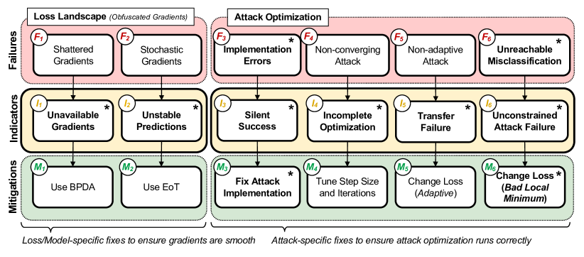
Figure 1: Indicators of Attack Failure (IoAF). We show the connections among the distinct attack failures (top), the proposed IoAF (center), and the corresponding mitigations (bottom). The novel failures, indicators, and mitigations found in this work are highlighted in bold and marked with “$\ast$”.

Attack-optimization Failures, Mitigations, and Indicators. The second category of failures is connected to problems encountered when running a gradient-based attack to solve the optimization problem given in Eq. (1)Problem (1)-(2) with Algorithm 1. This category encompasses failures $F_{3}$-$F_{6}$ in Fig. 3.
F₃: Implementation Errors. If the attack algorithm is unable to find adversarial examples, the implementation might be flawed. For example, we isolated a bug inside the PGD attack procedure proposed by Madry  [madry18-iclr]. This attack returns the We are the first to identify and characterize this failure, which affects many widely-used attack implementations and past evaluations. In particular, we find that many attacks return the last point sample of the attack path (line 1 of Algorithm 2.1) even if this point is non-adversarial, discarding potentially successful it is not adversarial, discarding valid adversarial examples found earlier along the optimization process in the attack path (F₃ in Fig. 3). Similarly, a recent work showed how This issue affects: (i) the PGD attack implementations [madry18-iclr] currently used in the four most-used Python libraries for crafting adversarial examples, i.e. , Foolbox, CleverHans, ART, and Torchattacks (for further details, please refer to A.7); and also (ii) AutoAttack [croce2020reliable]returns the original point when no adversarial examples are found. While this is not a problem per se, it becomes faulty when applied against a surrogate model and later transferred to the real target, since it will use the unperturbed point to calculate the adversarial robustness [croce2022evaluating]. , as it returns the initial sample if no adversarial example is found, leading to flawed evaluations when used in transfer settings [croce2022evaluating].
Once executed, attacks may not reach convergence (in Fig. 3). This problem can be caused by sub-optimal choices of the attack hyperparameters, including the step size $\alpha$ and the number of iterations $n$ (as shown in Algorithm 1). If $\alpha$ is too small, the gradient update step is not sufficiently exploring the space (line 1 of Algorithm 1), while using too few iterations $n$ might cause an early stopping of the attack (line 1 of Algorithm 1). An example of this failure can be found inthe evaluations of the defenses proposed by Buckmanet al. M₃: Fix Attack Implementation. To fix the issue, we propose to modify the optimization algorithm to return the best result. This mitigation can also be automated using the same mechanism used to automatically evaluate the IoAF, i.e. , by wrapping the attack algorithm with a function that keeps track of the best sample found during the attack optimization and eventually returns it.
I₃: Silent Success. We design $I_{3}(\boldsymbol{x})$ as a binary indicator that is set to $1$ when the final point in the path is not adversarial, but an adversarial example is found along the attack path (and $0$ otherwise).

F₄: Non-converging Attack. This failure is reported in [tramer2020adaptive], noting that the flawed evaluations performed by Buckman et al.  [buckman2018thermometer] and Panget al. [pmlr-v97-pang19a] et al.  [pmlr-v97-pang19a], respectively, where they respectivelyused only 7 and 10 steps of PGD for testing the robustness of their defense. The loss function that the attacker optimizes does not match the actual loss of the target system (their defenses. More generally, attacks may not reach convergence (F₄ in Fig. 3) . This failure might have different causes. One of them depends on a bad choice of the surrogate model due to inappropriate choices of their hyperparameters, including not only an insufficient number of iterations $n$ (line 1 1 of Algorithm 1), and it manifests when either the attack is (i) computed on a undefended model or a portion of the real target, and later tested against the defense; or (ii)the target model is not differentiable, and the chosen surrogate does not correctly approximate it. Another cause lays in the choice of an attack with poor transferability performance, that are later tested on the real target [demontis2019adversarial] with no success. Since we consider all these cases, we differ from the literature where the term non-adaptive has been used only for attacks that were not specifically designed to target a given defense  [tramer2020adaptive]. An example of this failure is found in the evaluation of Das et al. [das2018shield], where they attack an undefended model, and then evaluated the robustness by directly applying these adversarial examples on the defended model. but also an inadequate step size $\alpha$ (line 1 of Algorithm 1).

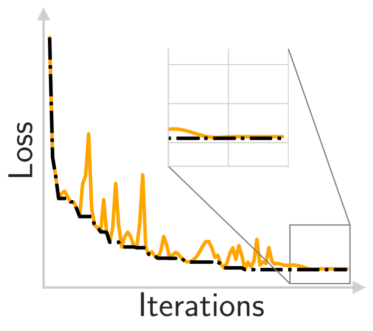
Figure 2: I₄ indicator.

M₄: Tune Step Size and Iterations. The failure can be patched by increasing either the step size $\alpha$ or the number of iterations $n$.
The attack runs, it does not encounter any other failure, but it converges to a local minimum without finding any adversarial misclassification (I₄: Incomplete Optimization. To automatically evaluate if the attack has not converged, we propose a novel indicator that builds a monotonically decreasing curve $\hat{L}$ for the loss, by keeping track of the best minimum found at each attack iteration (a.k.a. cumulative minimum curve, shown in black in Fig. 2). Then, we compute the relative loss decrement $D(\boldsymbol{x})$ in the last $k$ iterations (out of $n$) as: $D(\boldsymbol{x})=|\hat{L}^{(n)}-\hat{L}^{(n-k)}|/(\max_{i}\hat{L}^{(i)}-\min_{i}\hat{L}^{(i)})\in[0,1]$ . We set $I_{4}(\boldsymbol{x})=1$ if $D(\boldsymbol{x})\geq\mu$ (and 0 otherwise). In our experiments, we set the parameters $k=10$ and $\mu=1\%$, as detailed in Sect. 3.

F₅: Non-adaptive attack. This failure is only qualitatively discussed in [athalye18-iclr, carlini2019evaluating, tramer2020adaptive], showing that many previously-published defenses can be broken by developing adaptive attacks that specifically target the given defense mechanism. However, to date, it is still unclear how to evaluate if an attack is really adaptive or not (as it is mostly left to a subjective judgment). We try to shed light on this issue below. We first note that this issue arises when existing attacks are executed against defenses that may either have non-differentiable components [das2018shield] or use additional detection mechanisms [meng17-ccs]. In both cases, the attack is implicitly executed in a transfer setting against a surrogate model which retains the main structure of the target, but ignores the problematic components/detectors; e.g. , Das et al.  [das2018shield] simply removed the JPEG compression component from the model. However, it should be clear that optimizing the attack against such a bad surrogate $\hat{\boldsymbol{\theta}}$ (line 1 of Algorithm 1) is not guaranteed to also bypass the target model $\boldsymbol{\theta}$ (F₅ in Fig. 3).Since we already have excluded the presence of gradient obfuscation, the causes of this failure are hidden in the combination of both the objective function and the optimizer used to reach the goal, that is not successfully explore the loss landscape of the target model
M₅: Change Loss (Adaptive). Previous work [athalye18-iclr, carlini2019evaluating, tramer2020adaptive] applied custom fixes by using better approximations of the target, i.e. , loss functions and surrogate models that consider all the components of the defense in the attack optimization. This is unfortunately a non-trivial step to automate.
I₅: Transfer Failure. Despite the failure and some qualitative ideas to implement mitigations being known, it is unclear how to measure and evaluate if an attack is really adaptive. To this end, we propose an indicator that detects F₅ by evaluating the misalignment between the loss $L$ optimized by the attack on the surrogate $\hat{\boldsymbol{\theta}}$ and the same function evaluated on the target $\boldsymbol{\theta}$. We thus set $I_{5}(\boldsymbol{x})=1$ if the attack sample bypasses the surrogate but not the target model (and $0$ otherwise).

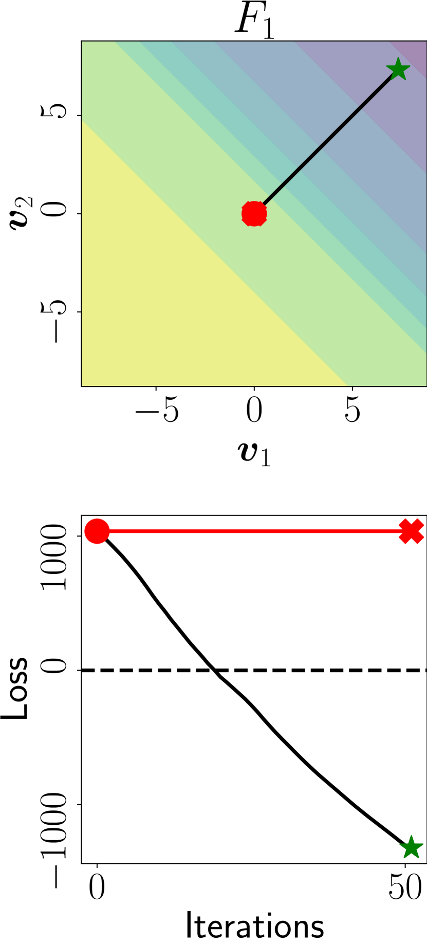
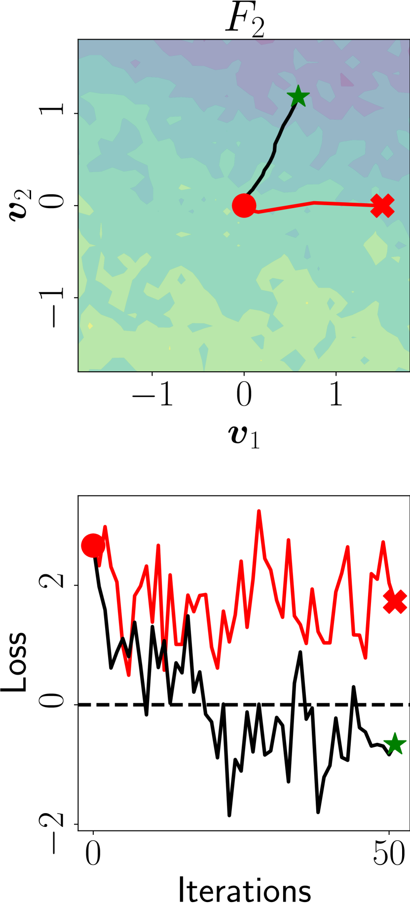
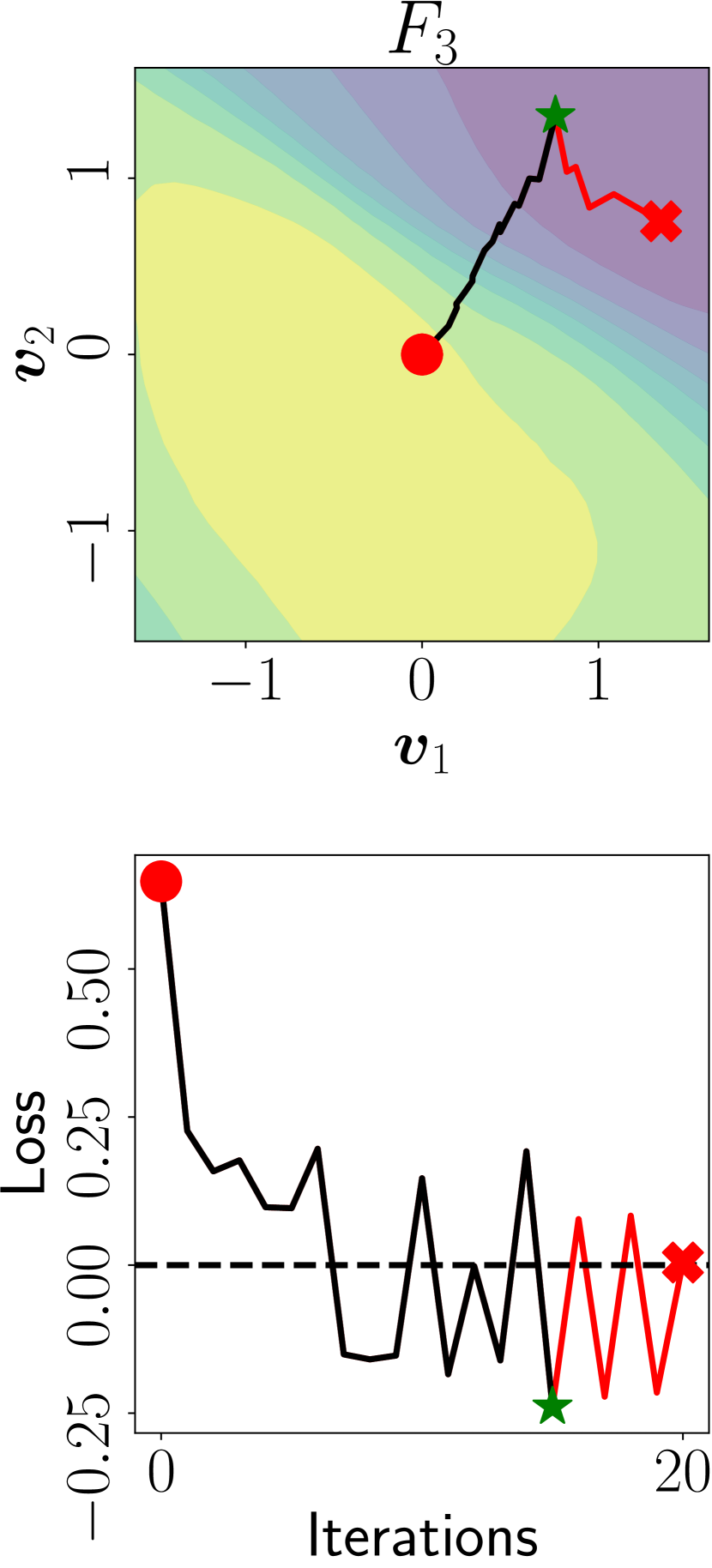
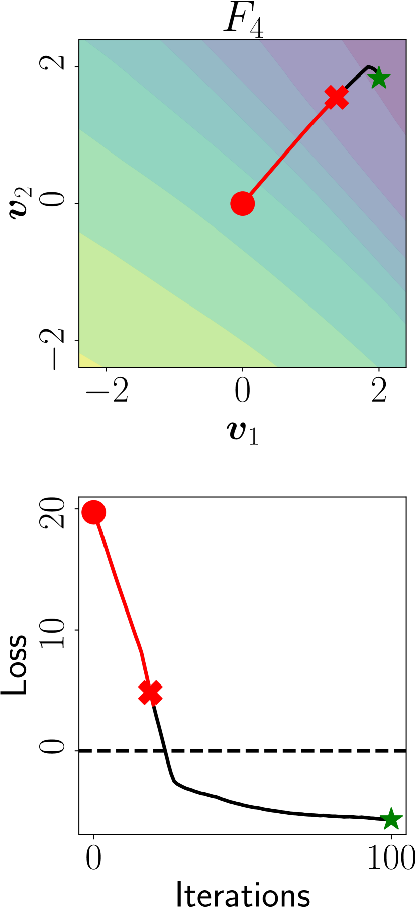
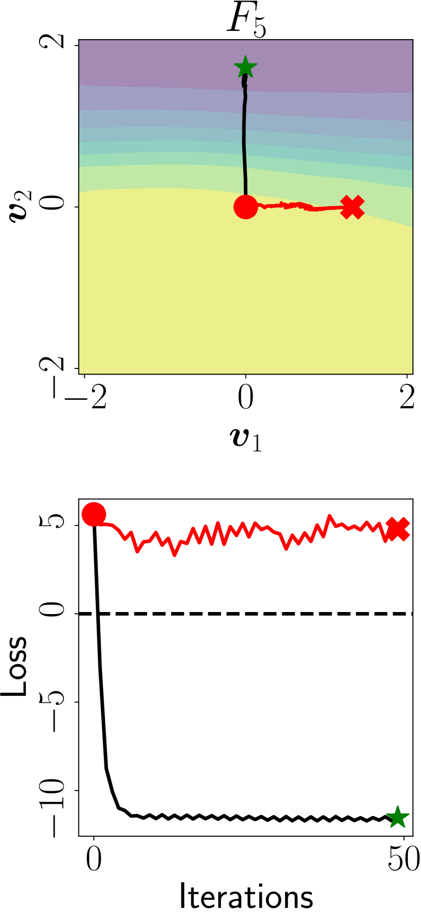
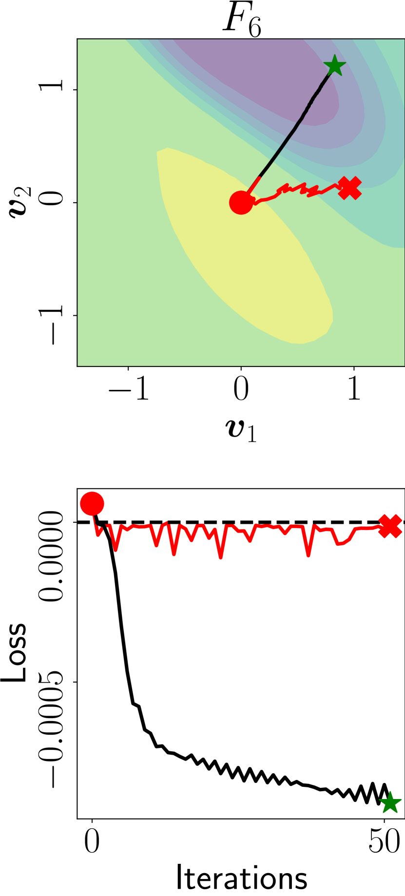
Figure 3: The six attack failures that can be encountered during the optimization of an attack. The failed attack path is shown in grayred, while the successful attack is displayed in black. The point $\boldsymbol{x}_{0}$ is marked with the red dot, the returned point of the failed attack with a red cross, and the successful adversarial point with the green star. The top row shows the loss landscape, as $L(\boldsymbol{x}+a\boldsymbol{v}_{1}+b\boldsymbol{v}_{2},y_{i};\boldsymbol{\theta})$. $\boldsymbol{v}_{1}$ is the normalized direction $(\boldsymbol{x}_{n}-\boldsymbol{x}_{0})$, while $\boldsymbol{v}_{2}$ is a representative direction for the displayed case. In the second row we show the value of $L(\boldsymbol{x}+\boldsymbol{\delta}_{i},y_{i};\boldsymbol{\theta})$ for the evaluated model.

3 Indicators of Attack Failure

Indicators of Attack Failures. The top row lists the six general failures encountered in gradient-based attacks. The second row lists the Indicators of Attack failures we propose, and the last row depicts possible mitigations that can be applied.

We now introduce the Indicators of Attack Failure (IoAF): metrics that quantify the presence of failures in the robustness evaluations of machine-learning models. For each indicator, we also identify suitable fixes that can be applied when failures are detected, as summarized in Fig. 1.

This indicator detects the presence of non-differentiable components or numerical instabilities when computing gradients (). The indicator computes the gradient of the loss of the attack a batch of 10 input samples, triggering if at least one of them has zero norm or if the gradient computation returns an error.This indicator quantifies the high variability of the loss landscape, caused by the the presence of noisy gradients (). We hence measure how much the CE loss of the model’s predictions varies in absolute value when sampled from an $\ell_{2}$-ball with a radius comparable to the step size, centered on an input sample. Let $L_{0}$ be the loss at the center of this ball, and $L_{1}...L_{n}$ the sampled values, the indicator is computed as $\min(\frac{1}{n}\sum_{i=1}^{n}|(L_{0}-L_{i})/L_{0}|,1)$. We repeat this computation on a batch of 10 samples, and the indicator signals the failurewhen the mean fluctuation exceeds the 10% of the original value. Such a threshold has been decided by observing the empirical results of our work, and that value already signals the presence of the failure.This indicator is designed as a binary flag that triggers when the final point in the path is non-adversarial, but a legitimate F₆: Unreachable Misclassification. We are the first to identify and characterize this failure. It assumes that gradient-based attacks can get stuck in bad local minima (e.g. , characterized by flat regions), where no adversarial example is found inside the attack path, as described by the implementation errors failure ().indicator. This indicator quantifies the non-convergence of the attack ()caused by flawed choices for the number of iterations and the step size. Intuitively, a well-converged attack is characterized by negligible improvement of the objective in the last iterations. This indicator builds a monotonically decreasing curve, by keeping track of the best minimum found at each iteration of the attack, as pictured in Fig. 2. Then, the indicator computes the decrement of the loss of the last 10 iterations, and it returns 1 if it does not decrease by at least 1%. Again, this threshold has been decided by observing the results of our experimental analysis(F₆ in Fig. 3). When this failure is present, unconstrained attacks (i.e. , attacks with $\epsilon\rightarrow\infty$ in Eq. 2) are also expected to fail, even if adversarial examples exist for sure in this setting (since the feasible domain includes samples from all classes).
This indicator looks for the non-adaptive failure () by measuring if the attack fails against the target model while succeeding against the surrogate one. If the attacktransfers successfully, the indicator is set to 0, otherwise it is set to 1.M₆: Change Loss (Bad Local Minimum). We argue that this failure can be fixed by modifying the loss function optimized by the attack, to avoid attack paths that lead to bad local minima. However, similarly to M₅ , this is not a trivial issue to fix, and it is definitely not easy to automate.
I₆: Unconstrained Attack Failure. This indicator demonstrates the inability of the optimizer Despite being difficult to find a misclassification even when using an unbounded perturbation (suitable mitigation for F₆ ). This configuration should always lead to successful attacks as the optimization algorithm has no constraints [carlini2019evaluating]. To measure such behavior, we re-compute adversarial attacks on a set of 10 points by setting an infinite perturbation bound. Hence, this indicator returns 1 if at least one of these attacks fails , detecting it is straightforward. To this end, we run an unconstrained attack on the given input $\boldsymbol{x}$, and we set $I_{6}(\boldsymbol{x})=1$ if such an attack fails (and $0$ otherwise).

2.1 Fixing FailuresWe now propose a systematic evaluation protocol that leverages the output of our indicators of attack failure to improve the reliability of robustness evaluations . Mitigating Loss Landscape Failures. The evaluation should ensure that the objective function is smooth enough to be explored by the attackalgorithm. Hence, the loss landscape failures should be mitigated first, to improve the likelihood of the attack succeeding.How to Use Our Framework

We summarize here the required steps that developers and practitioners should follow to debug their robustness evaluations with our IoAF.
If is active, one of the functions composed to compute the model ’s predictions $f=f_{K}\circ\ldots\circ f_{i}\circ\ldots\circ f_{1}$ is affecting the computation of the input gradient $\nabla_{\boldsymbol{x}}f(\boldsymbol{x})=\frac{\partial f_{K}}{\partial f_{K-1}}\circ\ldots\circ\frac{\partial f_{i}}{\partial f_{i-1}}\circ\ldots\circ\frac{\partial f_{1}}{\partial x}$, as it may either be non-differentiable, or cause numerical instabilities. In this case, the Backward Pass Differentiable Approximation (BPDA) [athalye18-iclr] can be used to approximate the derivative of the problematic function $f_{i}$ as $\frac{\partial f_{i}}{\partial f_{i-1}}=\mathbf{I}$, being $\mathbf{I}$ the identity matrix(1) Initialize Evaluation. The evaluation is initialized with a chosen attack, along with its hyperparameters, number of samples, and the model to evaluate.
If is active, the computed gradients point towards uninformative, random directions that cause the attackto fail. This issue is fixed by applying the Expectation over Transformation (EoT) technique [athalye18, tramer2020adaptive], which smooths the attack loss $L$ as $\hat{L}=\frac{1}{\gamma}\sum_{i=1}^{\gamma}L(\boldsymbol{x}+\boldsymbol{\delta}_{i},y;\boldsymbol{\theta})$, where $\boldsymbol{\delta}_{i}$ is sampled from an isotropic Normal distribution $\mathcal{N}(\boldsymbol{0},\sigma^{2}\mathbf{I})$. The parameters $\sigma$ and $\gamma$ have to be chosen based on the problem at hand, to provide sufficiently-informative gradients.

Mitigating Attack Optimization Failures. Once the issues related to gradient obfuscation are solved, we can focus on fixing the failures encountered during the (2) Mitigate Loss-landscape Failures. Before computing the attackoptimization. , the evaluation should get rid of loss-landscape failures, by computing I₁ and I₂ , and applying M₁ and M₂ accordingly.
If is active, adversarial examples are correctly computed but they are not exploitable since the implementation is flawed.Hence, such attack implementation must be fixed accordingly, by ensuring that the optimization algorithm returns the best result.These indicators are computed on a small random subset of $N$ samples, as the presence of either F₁ or F₂ would render useless the execution of the attack on all points. Both F₁ and F₂ are reported if they are detected on at least one sample in the given subset.
If is active, it means that the optimization result can still be improved, and hence both the step size and the number of iterations can be increased(3) Run the Attack. If F₁ and F₂ are absent or have been fixed, the attack can be run on all samples.
(4) Mitigate Attack-specific Failures. Once the attack completes its execution, indicators I₃ , I₄ and I₅ should be checked. Depending on their output, M₃ , M₄ , and M₅ are applied, and the attack is repeated (on the affected samples). If is active, the attack should be repeated upon changing the surrogate to better approximate the target, choosing a stronger attack, or including the defense inside the attack objective itself [tramer2020adaptive]. This step implies repeating the previous debugging steps and thus ensuring that the new attack is not suffering from the previous failures. If no failures are found, but the attack is still failing, the value of I₆ should be checked, and M₆ applied if needed. As I₁ and I₂ , I₆ is active, the chosen optimization algorithm is not exploring sufficiently the loss landscape of the model. Hence, the evaluation should be repeated with a better attack strategy that converges to adversarial examples when the hard constraints are removed, like applying the normalization of the gradient norm  [sotgiu2020deep, Yu_2019_NeurIPSweakness]. is also computed on a subset of $N$ samples to avoid unnecessary computations. The failure is reported if $\textit{I\textsubscript{6}}=1$ for at least one sample.

Let us finally remark that , when no indicator triggers, one should not conclude that robustness may not be worsened by a different, more powerful attack. This is indeed a problem of any empirical evaluation, including software testing – which does not ensure that software is bug-free, but only that some known issues get fixed. Our methodology, similarly, highlights the presence of known failures in adversarial robustness evaluations , and suggests how to mitigate them with a systematic protocol, taking a first concrete step towards toward making robustness evaluations more systematic and reliable.

3 Experiments

We now demonstrate the efficacy of our indicators, In this section, we demonstrate the effectiveness of our approach by re-evaluating the robustness of $7$ defenses, and using our IoAF framework to fix them. We also conduct the following additional experiments, reported in the appendix: (i) we describe how we set the thresholds $\tau$ for I₂ and $\mu$ for I₄ in A.2; (ii) we evaluate 6 more robust image classification models, discovering that their robustness claims might be unreliable in A.3; and (iii) we offer evidence that IoAF can encompass perturbation models beyond $\ell_{p}$ norms by analyzing the robustness evaluations of selected models through the lens of our methodologyone Windows malware detector in A.4, one Android malware detector in A.5, and one audio keyword-spotting model in A.5.

Experimental Setup. We run our attacks on an Intel^® Xeon^® CPU E5-2670 v3, with 48 cores, 126 128 GB of RAM, equipped with a Nvidia Quadro M6000 with 24 GB of memory, and we leverage the SecML library [pintor2022secml] to implement our methodology. We show failures of gradient-based attacks on 7 previously published defenses [das2018shield, guo2018countering, papernot16-distill, xiao2019resisting, pmlr-v97-pang19a, Yu_2019_NeurIPSweakness, sotgiu2020deep, robustness, zagoruyko2016wide], by inspecting them with our evaluation protocol. Most of these modelsIoAF, and most of them [das2018shield, guo2018countering, papernot16-distill, xiao2019resisting, pmlr-v97-pang19a, Yu_2019_NeurIPSweakness] are characterized by wrong robustness evaluations, hindered by failures that spread a false sense of security among the community. . We choose these defenses in particular because it is known that the original evaluation is their original evaluations are incorrect [athalye18, tramer2020adaptive]; our goal here is to show that our framework would have been able to identify these errorsin the first place even before performing a correct attack. Additionally, we show how our framework could have been used to fix the original attack evaluation for the encountered issues, offering a more accurate robustness evaluation. We also IoAF would have identified and mitigated such errors. We include the evaluation of an adversarial detector [sotgiu2020deep] to highlight that our framework IoAF is able to detect possible failures of this family of classifiers. Lastly, we We include the robustness evaluations of a Wide-ResNet [zagoruyko2016wide] and an adversarially-trained model [robustness], to highlight that our indicators do not trigger when they inspect sound evaluations. We defer details of the selected original evaluations to the Appendix. To A.1. Lastly, to demonstrate that automated attacks do not provide guarantees on performing correct evaluations (without human intervention), we also apply the AutoPGD attack [croce2020reliable] with two different loss functions, namely the Cross-Entropy loss (APGD_CE) and the Difference of Logits Ratio (APGD_DLR). Robustness is computed with the robust accuracy (RA) metric, quantified as the ratio of samples classified correctly within a given perturbation bound $\epsilon$. For I₁ , I₂ , and I₆ we set $N=10$, and for I₄ we set $k=10$. For I₂ , we set the number of sampled neighboors $s=100$, and the radius of the $\ell_{2}$ ball $r=10^{-3}$, to match the step size $\alpha$ of the evaluations. The thresholds $\tau$ of I₂ and $\mu$ of I₄ are set to $10\%$ and $1\%$ respectively (details about their calibration in A.2). All the robustness evaluations are performed on a pool of 100 samples from the test dataset of the considered model, and for each attack we evaluate the robust accuracy with $\epsilon=8/255$ for CIFAR models, and $\epsilon=0.5$ for the MNIST ones. The step size $\alpha$ is set to match the original evaluations (as detailed in  A.1).

Table 1: Indicator values (cols.) computed on the selected models (rows) using different attacks. The robust accuracy (RA) is reported in the last column (best values in bold). The symbol "Tr" denotes a transfer attack. The $\checkmark$ represents the detection of a specific failure. We report in parentheses the mean indicator value for , and the fraction of samples which triggered the indicator for which indicators I₂ , I₃, I₄, and I₆ are active.

Model	Attack	I1	I2	I3	I4	I5	I6	RA
ST	PGD							0.00
ADV-T	PGD							0.48
DIST	Original	$\checkmark$					$\checkmark$(10/10)	0.95
	APGDCE	$\checkmark$					$\checkmark$(10/10)	0.99
	APGDDLR							0.00
	Patched							0.01
k-WTA	Original		$\checkmark$(10/10)	$\checkmark$(23%)	$\checkmark$(11%)		$\checkmark$(4/10)	0.67
	APGDCE		$\checkmark$(10/10)		$\checkmark$(21%)		$\checkmark$(2/10)	0.35
	APGDDLR		$\checkmark$(10/10)				$\checkmark$(4/10)	0.28
	Patched				$\checkmark$(6%)		$\checkmark$(2/10)	0.09
IT	Original		$\checkmark$(10/10)	$\checkmark$(33%)	$\checkmark$(90%)			0.32
	APGDCE		$\checkmark$(10/10)	$\checkmark$(3% )			$\checkmark$(2/10)	0.12
	APGDDLR		$\checkmark$(10/10)	$\checkmark$(5%)			$\checkmark$(1/10)	0.12
	Patched				$\checkmark$(3%)			0.00
EN-DV	Original				$\checkmark$(100%)		$\checkmark$(3/10)	0.48
	APGDCE							0.00
	APGDDLR							0.00
	Patched							0.00
TWS	Original				$\checkmark$(74%)	$\checkmark$(6%)	$\checkmark$(8/10)	0.77
	APGDCE							0.03
	APGDDLR						$\checkmark$(7/10)	0.68
	Patched				$\checkmark$(1%)			0.01
JPEG-C	Original	$\checkmark$						0.85
	Original (Tr)					$\checkmark$(78%)		0.74
	APGDCE (Tr)					$\checkmark$(62%)		0.51
	APGDDLR (Tr)					$\checkmark$(85%)		0.70
	Patched							0.01
DNR	Original				$\checkmark$(100%)		$\checkmark$(10/10)	0.75
	APGDCE				$\checkmark$(3%)			0.02
	APGDDLR						$\checkmark$(2/10)	0.20
	Patched				$\checkmark$(1%)			0.03

Identifying and Fixing Attack Failures. We now delve into the description of the considered evaluations, which failures we detect and how we patch mitigate them, reporting the results in Table 1.

Correct Evaluations (ST, ADV-T). We first evaluate the robustness analysis of the Wide-ResNet and the adversarially-trained model, by applying PGD with CE loss, with $n=100$ (number of steps) and $\alpha=0.03$ (step size). Since no gradient obfuscation techniques have been used, the loss landscape indicators do not trigger. Also, since the attacks smoothly converge, these evaluations do not trigger any attack optimization indicator. Their robust accuracy is, respectively, 0% and 48%.

Defensive Distillation (DIST). Papernot et al. [papernot16-distill] use distillation to train a classifier to saturate the last layer of the network, making the computations of gradients numerically unstable and impossible to calculate, triggering the I₁ indicator, but also I₆ indicator as the optimizer can not explore the space. To patch this evaluation, we apply M₁ to overcome the numerical instability caused by DIST, forcing the attack to leverage the logits of the model instead of computing the softmax. Such a fix reduces the robust accuracy from 95% to 1%. In contrast, APGD_DLR manages to decrease the robust accuracy to 0%, as it avoids the saturation issue by considering only the logits of the model, while APGD_CE triggers the same issues of the original evaluation.

k-Winners Take All (k-WTA). Xiao et al. [xiao2019resisting] develop a classifier with a very noisy loss landscape, that destroys the meaningfulness of the directions of computed gradients. The original evaluation triggers I₂, since the loss landscape is characterized by frequent fluctuations, but also I₃, as the applied PGD [madry18-iclr] returns the last point of the attack discarding adversarial examples found within the path. Moreover, due to the noise, the attack is not always reaching convergence, as signaled by I₄, also performing little exploration of the space, as flagged by I₆. Hence, we apply M₂, performing the EoT on the loss of PGD  [tramer2020adaptive] with $\gamma=2000$ and $\sigma=8/255$, we PGD loss, sampling 2000 points from a Normal distribution $\mathcal{N}(0,\sigma^{2}\mathbf{I})$, with $\sigma=8/255$. We fix the implementation with M₃, and increase the iterations with M₄, thus reducing the robust accuracy from 67% to 9%. However, our evaluation still triggers I₄ and I₆, implying that for some points the result can be improved further by increasing the number of steps or the smoothing parameter $\gamma$. Both APGD_CE and APGD_DLR trigger I₂, since they are not applying EoT, and they partially activate I₆, similarly to the original evaluation. Interestingly, APGD_DLR converges better than APGD_CE, as the latter triggers I₄. Both attacks decrease the robust accuracy to 35% and 28%, a worst estimate than the one computed with the patched attack that directly handles the presence of the gradient obfuscation.

Input Transformations (IT). Guo et al. [guo2018countering] apply random affine input transformations to input images, producing a noisy loss landscape that varies at each prediction, thus its original robustness evaluation I₂, I₃, and I₄ indicators, for the same reasons of k-WTA. Again, we apply M₂, M₃ and M₄, using EoT with $\gamma=200$ and $\sigma=8/255$, decreasing the robust accuracy from 32% to 0%. Still, for some points (even if adversarial) the objective could still be improved, as I₄ is active for them. Both APGD_CE and APGD_DLR are able to slightly decrease the robust accuracy to 12%, but they both trigger the I₂ and I₆ indicator since they are not addressing the high variability of the loss landscape.

Ensemble Diversity (EN-DV). Pang et al. [pmlr-v97-pang19a] propose an ensemble model, evaluated with only 10 steps of PGD, thus triggers the I₅ indicator since the attack is not reaching convergence. As a consequence, also the unbounded attack is failing, thus triggering I₆. We apply the M₄ mitigation and we set $n=100$, as already done by previous work [tramer2020adaptive]. This fix changes the robust accuracy from 48% to 0%. Not surprisingly, both APGD_CE and APGD_DLR are able to bring the robust accuracy to 0%, since they both automatically modulate the step size.

Turning a Weakness into a Strength (TWS). Yu et al. [Yu_2019_NeurIPSweakness] propose an adversarial example defense, composed of different detectors. For simplicity, we only consider one of these, and we repeat their original evaluation with PGD without the normalization operation on the computed gradients, and $n=50$. This attack does not converge, triggering I₄, and if fails to navigate the loss landscape due to the very small gradients, triggering also I₆. We apply M₄, by settint setting $n=100$, and we use the original implementation of PGD (with the normalization step), hence applying also M₆, achieving a drop in the robust accuracy from 77% to 1%. For only one point, our evaluation triggers I₄, as better convergence could be achieved. Moving forward, APGD_CE finds a robust accuracy of 3%, as it is modulating the step size along with using the normalization of the gradient. On the other hand, APGD_DLR triggers the I₆ indicator and the robust accuracy remains at 68%, as the attack is not able to avoid the rejection applied by the model.

JPEG Compression (JPEG-C). Das et al. [das2018shield] pre-process all input samples using JPEG compression, before feeding the input to the undefended network. We apply this defense on top of a model with a reverse sigmoid layer [lee2019defending], as was done in [yao2021automated]. The authors firstly state that they can not directly attack the defense due to its non-differentiability (thus triggering I₁), then they apply the DeepFool [moosavi16-deepfool] attack against the undefended model. This attack has low transferability, as it is not maximizing the misclassification confidence [demontis2019adversarial]. The robustness evaluation triggers I₅ since the attack computed on the undefended model is not successful on the real defense. To patch this evaluation, we apply M₁, approximating the back-propagation of the JPEG compression layer and the reverse sigmoid layers with BPDA [tramer2020adaptive], and we apply M₅ by using PGD to maximize the misclassification confidence of the model. This fix is sufficient to reduce its robust accuracy from 74% to 46%. However, is active, implying that the chosen BPDA strategy might be refined to get a better result. 0.01%. Since APGD can not attack non-differentiable models, we run the attack against the undefended target and we transfer the adversarial examples on the defense. However, both of them trigger I₅ as transfer attacks are not effective, keeping the robust accuracy to 51% and 70%.

Deep Neural Rejection (DNR). Sotgiu et al. [sotgiu2020deep] propose an adversarial detector encoding it as an additional class that captures the presence of attacks. Similarly to TWS, it was evaluated with PGD with no normalization of the norms of gradients. The attack does not converge, as it triggers I₄, but also sometimes gets trapped inside the rejection class, triggering I₆. Hence, we apply both M₄ and M₆, by increasing the number of iterations and considering an attack that avoids minimizing the score of the rejection class. These fixes reduce the robust accuracy from 75% to 3%. Interestingly, only APGD_CE is able to reduce the robust accuracy to 2%, also noting that it might be still beaten since it is triggering I₄. On the contrary, APGD_DLR is reducing the robust accuracy only to 20%, by also triggering I₆. By manually inspecting the outputs of the model, we found that its scores tend to have all the same values, due to the SVM-RBF kernel that assigns low prediction outputs to samples that are outside the distributions of the training samples. This causes the DLR loss to saturate due to the denominator becoming extremely small, making this attack weak against the DNR defense.

4 Related Work

Robustness Evaluations. Prior work focused on analyzing the quality of robustness evaluations of selected re-evaluating already-published defenses[carlini17-aisec, athalye18, tramer2020adaptive, carlini2019evaluating], by inspecting and correcting their over-emphasized security claims with sound analysis. On top of this, the authors also suggest  [carlini17-aisec, athalye18, tramer2020adaptive, carlini2019evaluating], showing that their adversarial robustness was significantly overestimated. The authors then suggested qualitative guidelines and best practices to avoid repeating the mistakes of past robustness evaluationssame evaluation mistakes in the future. However, these can neither specify the reasons why the attacks fail nor be applied automatically on the tested defense. In contrast, our work is inspired by these suggestions, as it offers a systematic methodology to provide better robustness evaluations , also quantifying why and how attack fails. the application of such guidelines remained mostly neglected, due to the inherent difficulty of applying them in an automated and systematic manner. To overcome this issue, in this work we have provided a systematic approach to debug adversarial robustness evaluations via the computation of the IoAF, which identify and characterize the main causes of failure of gradient-based attacks known to date. In addition, we have provided a semi-automated protocol that suggests how to apply the corresponding mitigations in the right order, whenever possible.

Benchmarks. Instead of measuring the robustness of individual models as the prior re-evaluating robustness of previously-proposed defenses with an ad-hoc approach, as the aforementioned papers do, researchers of the community proposedbenchmarks that provide a complete evaluation framework that can be applied to any future defense, with the ultimate goal of understanding which technique is bettersome more systematic benchmarking approaches have been proposed. Ling et al. [ling-19-deepsec] propose have proposed DEEPSEC, a benchmark that tests several attacks against a wide range of defenses. However, this framework was shown to be flawed by several implementation issues and problems in the configuration of the attacks [carlini2019critique]. Croce et al. [croce2020robustbench] propose RobustBench [croce2020robustbench]have proposed RobustBench, a benchmark that accepts state-of-the-art models as submissionsthat are automatically tested , and tests them automatically with AutoAttack [croce2020reliable]. Also, the same authors recently introduced alerts inside AutoAttack, displaying textual warnings The same authors have also recently introduced some textual warnings when executing AutoAttack, which are displayed if the strategy encounters specific issues (e.g. , randomness and zero gradients), taking inspiration from what we have done more systematically in this paper. Yao et al. [yao2021automated] propose the Adaptive AutoAttack evaluation protocol, that have proposed an approach referred to as Adaptive AutoAttack, which automatically tests a variety of attacks, by applying different configurations of parameters and objective functions, hence extending the procedure proposed by AutoAttack. This approach has been shown to outperform AutoAttack by some margin, but at the expense of being much more computationally demanding.

While all these protocols approaches are able to automatically compute security evaluations and rank defenses by their evaluate adversarial robustness, they are just applying attacks one after the other, hence missing either the real rationale behind attack failures or possible flaws of the applied techniques, spreading again a false sense of security. In contrast, our methodology improves these processes, as we are able to detect and patch faults encountered while computing adversarial mostly blindly apply different attacks to show that the robust accuracy of some models can be decreased by a small fraction. None of the proposed benchmarks has implemented any mechanisms to detect known failures of gradient-based attacks and use them to patch the evaluations, except for the aforementioned warnings present in AutoAttack, and a recent flag added to RobustBench. This flag reports a potentially flawed evaluation when the black-box (square) attack finds lower robust accuracy values than the gradient-based attacks , hence improving the evaluation protocol. Here we imagine that our framework could be used to help these tools automatically detect when their evaluationsare incomplete so that they could flag potential errors that should be investigatedAPGD_CE , APGD_DLR , and FAB. However, this is not guaranteed to correctly detect all flawed evaluations, as finding adversarial examples with black-box attacks is even more complicated and computationally demanding. Our approach finds the same issues without running any computationally-demanding black-box attack, but just inspecting the failures in the optimization process of gradient-based attacks. For these reasons, we firmly believe that our approach based on the IoAF will be extremely useful not only to debug in a more systematic and automated manner future robustness evaluations, but also to improve the current benchmarks.

5 Contributions, Limitations and Future Work

In this work, we propose the Indicators of Attack Failures (IoAF), quantitative tests that help debug failures of have proposed the first automated testing approach that helps debug adversarial robustness evaluations. We use them to develop a pipeline that detects and suggests how to mitigate the encountered failures , improving the reliability of adversarial robustness evaluations. To demonstrate that our indicators are useful, we select 7 defenses that have been previously shown to be weak against adversarial attacks, and we assess the reliability of their original evaluations using our indicators. We find that our methodology would have identified errors in all of these broken defenses, and could have predicted that future attacks would break them., by characterizing and quantifying four known and two novel causes of failures of gradient-based attacks. To this end, we have developed six Indicators of Attack Failure (IoAF), and connected them with the corresponding (semi-automated) fixes. We have demonstrated the effectiveness of our methodology by analyzing more than 15 models on three different domains, showing that most of the reported evaluations were flawed, and how to fix them with the systematic protocol we have defined.

An inherent limitation of our methodology is that, similarly to software testing, it does not ensure that an evaluation is failure-free, but only that none of the known failures we characterize and measure is present. It is indeed not possible to guarantee that a gradient-based attack has found the global optimum of a non-convex optimization problem. This is however a general limitation of empirical evaluations . We nevertheless believe that our set of indicators may also help unveil novel kinds of failure, e.g., if attacks with unbounded perturbation keep failing even after fixes are applied, thereby fostering the development of novel mitigations and indicators that will help extend our framework and improve it in the future.

Another avenue An interesting direction for future work is to further automate our analysis, by systematizing the steps required to make an attack adaptiveto the defensewould be to define mitigations that can be applied in a fully-automated way, including how to make attacks adaptive. Still, our work provides a set of debugging tools and systematic procedures that aim to significantly reduce the number of manual interventions and the required skills to detect and fix flawed robustness evaluations. We

To conclude, we firmly believe that integrating our work in current attack libraries and benchmarks will help avoid factual mistakes in adversarial robustness evaluations which have substantially hindered the development of effective defense mechanisms against adversarial examples thus far.

Checklist

1. For all authors…

   1. Do the main claims made in the abstract and introduction accurately reflect the paper’s contributions and scope? [Yes]

   2. Did you describe the limitations of your work? [Yes] We discuss the limitations in Sect. 5.

   3. Did you discuss any potential negative societal impacts of your work? [Yes] In Sect. 5, we specified that the aim of our work is not to break defenses in an harmful way. Our purpose is only to help researchers improving their security evaluation.

   4. Have you read the ethics review guidelines and ensured that your paper conforms to them? [Yes]

2. If you are including theoretical results…

   1. Did you state the full set of assumptions of all theoretical results? [N/A]

   2. Did you include complete proofs of all theoretical results? [N/A]

3. If you ran experiments…

   1. Did you include the code, data, and instructions needed to reproduce the main experimental results (either in the supplemental material or as a URL)? [Yes] The code will be submitted as supplementary material, and the instructions for reproducing the experiments are described in Sect. 3.

   2. Did you specify all the training details (e.g., data splits, hyperparameters, how they were chosen)? [Yes] We describe the experimental protocol in Sect. 3.

   3. Did you report error bars (e.g., with respect to the random seed after running experiments multiple times)? [N/A]

   4. Did you include the total amount of compute and the type of resources used (e.g., type of GPUs, internal cluster, or cloud provider)? [Yes] The resourced used for the experiments are listed in Sect. 3.

4. If you are using existing assets (e.g., code, data, models) or curating/releasing new assets…

   1. If your work uses existing assets, did you cite the creators? [Yes] We cited all the existing assets used for the experiments.

   2. Did you mention the license of the assets? [Yes] We cited the authors of the assets, and we provide the list of external assets along with the code.

   3. Did you include any new assets either in the supplemental material or as a URL? [Yes] We provide the code for computing the metrics as supplementary material.

   4. Did you discuss whether and how consent was obtained from people whose data you’re using/curating? [N/A] All the assets we used are publicly available.

   5. Did you discuss whether the data you are using/curating contains personally identifiable information or offensive content? [N/A]

5. If you used crowdsourcing or conducted research with human subjects…

   1. Did you include the full text of instructions given to participants and screenshots, if applicable? [N/A]

   2. Did you describe any potential participant risks, with links to Institutional Review Board (IRB) approvals, if applicable? [N/A]

   3. Did you include the estimated hourly wage paid to participants and the total amount spent on participant compensation? [N/A]

Appendix

Appendix A Appendix

Additional Details on Models and Original Evaluations

A.1 Additional Details on Models and Original Evaluations

We collect here the implementation details of the models considered in our experimental analysis, along with their original evaluations used to determine their adversarial robustness.

Distillation (DIST). Papernot et al. [papernot16-distill], develop a model to have zero gradients around the training points. However, this technique causes the loss function to saturate and produces zero gradients for the Cross-Entropy loss, but the defense was later proven ineffective when removing the Softmax layer [carlini2016defensive]. We re-implemented such defense, by training a distilled classifier on the MNIST dataset to mimic the original evaluation. Then, we apply the original evaluation, by using $\ell_{\infty}$-PGD  [madry18-iclr], with step size $\alpha=0.01$, maximum perturbation $\epsilon=0.3$ for 50 iterations on 100 samples, resulting in a robust accuracy of 95%.

k-Winners-Take-All (k-WTA). Xiao et al. [xiao2019resisting] propose a defense that applies discontinuities on the loss function, by keeping only the top-k outputs from each layer. This addition causes the output of each layer to drastically change even for very close points inside the input space. Unfortunately, this method only causes gradient obfuscation that prevents the attack optimization to succeed, but it was proven to be ineffective by leveraging more sophisticated attacks [tramer2020adaptive]. We leverage the implementation provided by Tramèr et al.. [tramer2020adaptive] trained on CIFAR10, and we replicate the original evaluation by attacking it with $\ell_{\infty}$-PGD [madry18-iclr] with a step size of $\alpha=0.003$, maximum perturbation $\epsilon=0.031$ and 50 iterations, scoring a robust accuracy of 67% on 100 samples.

Input-transformation Defense (IT). Guo et al. [guo2018countering] propose to preprocess input images with random affine transformations, and later feed them to the neural network. This preprocessing step is differentiable, thus training is not affected by these perturbations, and the network should be more resistant to adversarial manipulations. Similarly to k-WTA, this model is also affected by a highly-variable loss landscape, leading to gradient obfuscation [athalye18-iclr], again proven to be ineffective as a defense [tramer2020adaptive]. We replicate the original evaluation, by attacking this defense with PGD [madry18-iclr] with $\alpha=0.003$, with 10 iterations and a maximum perturbation of $0.031$, scoring 32% of robust accuracy.

Ensemble diversity (EN-DV). Pang et al. [pmlr-v97-pang19a] propose a defense that is composed of different neural networks, trained with a regularizer that encourages diversity. This defense was found to be evaluated with a number of iterations not sufficient for the attack to converge [tramer2020adaptive]. We adopt the implementation provided by Tramèr et al. [tramer2020adaptive]. Then, following its original evaluation, we apply $\ell_{\infty}$-PGD [madry18-iclr], with step size $\alpha=0.003$, maximum perturbation $\epsilon=0.031$ for 10 iterations on 100 samples, resulting in a robust accuracy of 48%.

Turning a Weakness into a Strength (TWS).Yu et al. [Yu_2019_NeurIPSweakness] propose a defense that applies a mechanism for detecting the presence of adversarial examples on top of an undefended model, measuring how much the decision changes locally around a sample. The authors evaluated this model with a self-implemented version of PGD that does not apply the sign operator to the gradients and hinders the optimization performance as the magnitude of the gradients is too small for the attack to improve the objective [tramer2020adaptive]. We apply this defense on a VGG model trained on CIFAR10, provided by PyTorch torchvision module . Following the original evaluation, we attack this model with $\ell_{\infty}$-PGD without the normalization of the gradients, with step size $\alpha=0.01$, maximum perturbation $\epsilon=0.031$ for 50 iterations on 100 samples, and then we query the defended model with all the computed adversarial examples, scoring a robust accuracy of 77%.

JPEG Compression (JPEG-C). Das et al. [das2018shield] propose a defense that applies the JPEG compression to input images, before feeding them to a convolutional neural network. The authors also study the variation of the robustness and clean accuracy by increasing or decreasing the level of compressionWe combine this defense with a defense from Lee et al.  [lee2019defending], originally proposed against black-box model-stealing attacks. This defense adds a reverse sigmoid layer after the model, causing the gradients to be misleading. This model was evaluated first directly, raising errors because of the non-differentiable transformation applied to the input, then re-evaluated with BPDA but with DeepFool, a minimum-distance attack, and finally found vulnerable to maximum-confidence attacks [athalye18-iclr]. We attack this model by replicating the original evaluation proposed by the author, and we first apply a standard PGD [madry18-iclr] attack that triggers the F₁ failures (as also mentioned by the author of the defense). Hence, we continue the original evaluation by applying the DeepFool attack against a model without the compression, with maximum perturbation $\epsilon=0.031$, 100 iterations on 100 samples. These samples are transferred to the defended model, scoring a robust accuracy of 85%.

Deep Neural Rejection (DNR). Sotgiu et al. [sotgiu2020deep] propose an adversarial detector built on top of a pretrained network, by adding a rejection class to the original output. The defense consists of several SVMs trained on top of the learned feature representation of selected internal layers of the original neural network, and they are combined to compute the rejection score. If this score is higher than a threshold, the rejection class is chosen as the output of the prediction. The defense was evaluated, similarly to TWS, with a PGD implementation not using the sign operator, leading the sample to reach regions where the gradients become unusable for improving the objective. This model was never found vulnerable by others, hence we are the first to show its evaluation issues. Following the original evaluation, we apply PGD without the normalization of gradients, with $\alpha=0.3$, 50 iterations with maximum perturbation $\epsilon=0.031$, and the scored robust accuracy is 75%.

A.2 Thresholding Indicators I₂ and I₄

We discuss here how to set the threshold values $\tau$ and $\mu$, respectively used to compute I₂ and I₄ .

For I₂ , we report the value of $V(\boldsymbol{x})$ for each model, averaged over the considered $N=10$ samples (along with its standard deviation) in Table LABEL:tab:i2_values. As one may notice, models with unstable/noisy gradients exhibit values higher than $0.4$, whereas non-obfuscated models exhibit values that are very close to $0$ (and the standard deviations are negligible). We set $\tau=10\%$ as the per-sample threshold in this case, but any other value between $0.1$ and $0.3$ would still detect the failure correctly on all samples. This threshold is thus not tight, but a conservative choice is preferred, given that missing a flawed evaluation would be far more problematic than detecting a non-flawed evaluation.

For I₄ , we report the mean value (and standard deviation) of $D(\boldsymbol{x})$ for each model and averaged over $N=10$ samples, in Table LABEL:tab:i4_values. Here, attacks that use few iterations (EN-DV ), and attacks that use PGD without the step normalization (TWS , DNR ) trigger the indicator. The evaluations that trigger already I₂ are not trusted as it is not worth checking convergence for models that present obfuscated gradients. Again, we used for I₄ a very conservative threshold to avoid missing the failure.

Table 2: Analysis of the threshold values $\tau$ and $\mu$ for indicators I₂ and I₄ .

	Mean $V(\boldsymbol{x})$	$I_{2}:V(\boldsymbol{x})$ $>\tau=10\%$
ST	0.02162 $\pm$ 0.00122
ADV-T	0.00059 $\pm$ 0.00003
DIST	0.00000 $\pm$ 0.00000
k-WTA	0.40732 $\pm$ 0.03256	$\checkmark$ (10/10)
IT	1.00000 $\pm$ 0.00000	$\checkmark$ (10/10)
EN-DV	0.00014 $\pm$ 0.00001
TWS	0.00862 $\pm$ 0.00080
JPEG-C	0.03129 $\pm$ 0.00152
DNR	0.00000 $\pm$ 0.00000

(a)

	Mean $D(\boldsymbol{x})$	$I_{4}:D(\boldsymbol{x})$ $>\mu=1\%$
ST	0.00279 $\pm$ 0.00778
ADV-T	0.00000 $\pm$ 0.00000
DIST	0.00000 $\pm$ 0.00000
k-WTA	0.04345 $\pm$ 0.10144	not trusted (I2 $\checkmark$ )
IT	0.00623 $\pm$ 0.01869	not trusted (I2 $\checkmark$ )
EN-DV	1.00000 $\pm$ 0.00000	$\checkmark$
TWS	0.16835 $\pm$ 0.10307	$\checkmark$
JPEG-C	0.00002 $\pm$ 0.00007
DNR	0.06857 $\pm$ 0.01660	$\checkmark$

(b)

A.3 Evaluation of Robust Image Classification Models

We evaluate 6 defenses recently published on top-tier venues, available through RobustBench [carmon2019unlabeled, sehwag2020hydra, wu2020adversarial, ding2019mma, rebuffi2021data] or their official repository [stutz2020confidence], by applying APGD_CE and APGD_DLR, using an $\ell_{\infty}$ perturbation bounded by $\epsilon=8/255$. We report the results in Table 3. Interestingly, we found that all these evaluations are unreliable, as they trigger the I₆ indicator. Hence, even without bounds on the perturbation model, the optimizer is unable to reach regions where adversarial examples are found. This suggests that applying M₆ , i.e. making the attacks adaptive, can improve the trustworthiness of these robustness evaluations.

Table 3: Indicator values (cols.) computed on the robust models (rows), using the APGD_CE and APGD_DLR attacks [croce2020reliable]. The robust accuracy (RA) is reported in the last column.

Model	Attack	I1	I2	I3	I4	I5	I6	RA
Stutz et al. [stutz2020confidence]	APGDCE						✓(10/10)	0.90
	APGDDLR						✓(10/10)	0.90
Carmon et al. [carmon2019unlabeled]	APGDCE						✓(4/10)	0.59
	APGDDLR						✓(3/10)	0.55
Sehwag et al. [sehwag2020hydra]	APGDCE						✓(4/10)	0.62
	APGDDLR						✓(4/10)	0.57
Wu et al. [wu2020adversarial]	APGDCE						✓(4/10)	0.62
	APGDDLR						✓(3/10)	0.59
Ding et al. [ding2019mma]	APGDCE						✓(2/10)	0.47
	APGDDLR						✓(2/10)	0.49
Rebuffi et al. [rebuffi2021data]	APGDCE						✓(4/10)	0.64
	APGDDLR						✓(5/10)	0.65

A.4 Application on Windows Malware

We replicate the evaluation of the MalConv neural network [raff2018malware] for Windows malware detection done by Demetrio et al.  [demetrio2021adversarial]. We used the "Extend" attack, which manipulates the structure of Windows programs while preserving the intended functionality [demetrio2021adversarial]. We replicate the same setting described in the paper by executing the Extend attack on 100 samples (all initially flagged as malware by MalConv), and we report its performances and the values of our indicators in Table 4. As highlighted by the collected results, this evaluation can be improved by using BPDA instead of the sigmoid applied on the logits of the model (M₁ ), and also by patching the implementation to return the best point in the path (M₃ ). Since MalConv applies an embedding layer to impose distance metrics on byte values (that have no notion of norms and distance), we need to adapt I₂ to sample points inside such embedding space of the neural network. Hence, the sampled values must then be projected back to byte values by inverting the lookup function of the embedding layer [demetrio2021adversarial]. However, this change to I₂ is minimal, and all the other indicators are left untouched.

Table 4: Indicator values (cols.) computed on the the Windows Malware use case, using the Extend attack from [demetrio2021adversarial]. The robust accuracy (RA) is reported in the last column.

Model	Attack	I1	I2	I3	I4	I5	I6	RA
MalConv	Extend	✓		✓(12%)			✓(3/10)	0.26

A.5 Application on Android Malware Detection

We replicate the evaluation of the Drebin malware detector by Arp et al.  [rieck14-drebin] from Demontis et al.  [demontis17-tdsc]. The considered attack only injects new objects into Android applications to ensure that feature-space samples can be properly reconstructed in the problem space. We limit the budget of the attack to include only 5 and 25 new objects, and we report the collected results in Table 5. The attack is implemented using the PGD-LS [demontis17-tdsc] implementation from SecML [pintor2022secml]. Note that, since the evaluated model is a linear SVM, the input gradient is constant and proportional to the feature weights of the model. Accordingly, the attack is successfully executed without failures.

Table 5: Indicator values (cols.) computed on the Android Malware use case, using the PGD-LS attack from [demontis17-tdsc]. The robust accuracy (RA) is reported in the last column.

Model	Attack	I1	I2	I3	I4	I5	I6	RA
SVM-ANDROID	PGD-LS (budget=5)							0.58
	PGD-LS (budget=25)							0.00

A.6 Application on Keyword Spotting

To demonstrate the applicability of our indicators to different domains, we applied our procedure to the audio domain, using a reduced version of the Google Speech Commands Dataset, including only the 4 keywords “up”, “down”, “left”, and “right”. We first convert the audio waveforms to linear spectrograms and then use these spectrograms to train a ConvNet (AUDIO-ConvNet) that achieves 99% accuracy on the test set. The spectrograms are then perturbed in the feature space using the PGD $\ell_{2}$ attack (in the feature space) and transformed back to the input space using the Griffin-Lim transformation [perraudin2013fast]. The samples are transformed again and passed through the network to ensure the attack still works after the reconstruction of the perturbed waveform. We leverage the PGD $\ell_{2}$ attack with $n=200$, $\alpha=5$, and $\epsilon=50$. Our indicators do not require any change to be applied to this domain. We report the values of our indicators and the robust accuracy in Table 6.

Table 6: Indicator values (cols.) computed on the keyword-spotting use case, using the PGD $\ell_{2}$ attack. The robust accuracy (RA) is reported in the last column.

Model	Attack	I1	I2	I3	I4	I5	I6	RA
AUDIO-ConvNet	PGD							0.00

A.7 Implementation Errors of Adversarial Machine Learning Libraries

As discussed in Sect. 2, we found F₃ in the PGD implementations of the most widely-used adversarial robustness libraries, namely Cleverhans (PyTorch, Tensorflow, JAX), ART (NumPy, PyTorch, and Tensorflow), Foolbox (EagerPy, which wraps the implementation of NumPy, PyTorch, Tensorflow, and JAX), Torchattacks (PyTorch). We detail further in Table 7 the specific versions and statistics. In particular, we report the GitHub stars (✰) to provide an estimate of the number of users potentially impacted by this issue. Let us also assume that there are a large number of defenses that have been evaluated with these implementations (or their previous versions, which most likely have the same problem). After this problem is fixed, all these defenses should be re-evaluated with the more powerful version of the attack, perhaps revealing faulty robustness performances.

Table 7: Versions and GitHub stars (✰) of the libraries where we found F₃.

Library	Version	GitHub ✰
Cleverhans	4.0.0	5.6k
ART	1.11.0	3.1k
Foolbox	3.3.3	2.3k
Torchattacks	3.2.6	984

A.8 Pseudo-code of Indicators

We report here the implementation of our proposed indicators. Since we write here a pseudo-code, we refer to the repository for the actual Python code.

Input : $\boldsymbol{x}$, input sample; $L(\cdot,y;\boldsymbol{\theta})$, the loss function of the attack with fixed label and model

Output : The value of I₁$(\boldsymbol{x})$

1 try :

2       return $\parallel\nabla_{x}L(\boldsymbol{x},y;\boldsymbol{\theta})\parallel_{\infty}=0$

3catch  gradient not computable:

4       return 1

Algorithm 2 Pseudo-code for the Unavailable Gradients indicator I₁$(\boldsymbol{x})$ .

Input : $\boldsymbol{x}$, input sample; $L(\cdot,y;\boldsymbol{\theta})$, the loss function of the attack with fixed label and model; $r$, noise radius; $s$, number of neighboring samples; $\tau$ threshold for triggering the indicator

Output : The value of I₂$(\boldsymbol{x})$

1

2$L^{(0)}\leftarrow L(\boldsymbol{x}_{j},y;\boldsymbol{\theta})$

3$\boldsymbol{x}^{(1)},...\boldsymbol{x}^{(s)}\sim\mathcal{U}(\boldsymbol{x}_{j}-\frac{r}{2}\mathbf{I},\boldsymbol{x}_{j}+\frac{r}{2}\mathbf{I})$

4$L^{(1)},...,L^{(s)}\leftarrow L(\boldsymbol{x}^{(1)},y;\boldsymbol{\theta}),...,L(\boldsymbol{x}^{(s)},y;\boldsymbol{\theta})$

5$V(\boldsymbol{x})\leftarrow\min(\frac{1}{s}\sum_{i=1}^{m}|(L^{(0)}-L^{(i)})/L^{(0)}|,1)$

6return $V(\boldsymbol{x})>\tau$

Algorithm 3 Pseudo-code for the Unstable Predictions indicator I₂$(\boldsymbol{x})$ .

Input : $\boldsymbol{x}$, the initial sample; $\boldsymbol{x}^{\star}$, the result returned by the attack; $\boldsymbol{\delta}_{0},...,\boldsymbol{\delta}_{n}$, the attack path; $\boldsymbol{\theta}$, the target model

Output : The value of I₃$(\boldsymbol{x})$

return $\boldsymbol{x}^{\star}$ is not adversarial for $\boldsymbol{\theta}$ and $\exists j\in[0,n]$ | $\boldsymbol{x}+\boldsymbol{\delta}_{j}$ is adversarial for $\boldsymbol{\theta}$

Algorithm 4 Pseudo-code for the Silent Success indicator I₃$(\boldsymbol{x})$ .

Input : $\boldsymbol{x}$, the initial sample; $\boldsymbol{\delta}_{0},...,\boldsymbol{\delta}_{n}$, the attack path; $L(\cdot,y;\boldsymbol{\theta})$, the loss function of the attack with fixed label and model; $k$, the length of the last part of the loss to retain;$\mu$ threshold for triggering the indicator

Output : The value of I₄$(\boldsymbol{x})$

1 $L^{(0)},...,L^{(n)}\leftarrow L(\boldsymbol{x}+\boldsymbol{\delta}_{0},y;\boldsymbol{\theta}),...,L(\boldsymbol{x}+\boldsymbol{\delta}_{n},y;\boldsymbol{\theta})$

2$L^{(0)},...,L^{(n)}\leftarrow$ rescale($L^{(0)},...,L^{(n)}$, $\left[0,1\right]$)

3$\hat{L}^{(0)},...,\hat{L}^{(n)}=$ cumulative-minimum$(L^{(0)},...,L^{(n)})$

4$D(\boldsymbol{x})\leftarrow\max(\hat{L}^{(n-k-1)},...,\hat{L}^{(n)})-\min(\hat{L}^{(n-k-1)},...,\hat{L}^{(n)})$

return $D(\boldsymbol{x})>\mu$

Algorithm 5 Pseudo-code for the Incomplete Optimization indicator I₄$(\boldsymbol{x})$ .

Input : $\boldsymbol{x}$, the initial sample; $\boldsymbol{x}^{\star}$, the result returned by the attack; $\boldsymbol{\delta}_{0},...,\boldsymbol{\delta}_{n}$, the attack path; $\boldsymbol{\theta}$, the target model; $\hat{\boldsymbol{\theta}}$, the model used for crafting the attack

Output : The value of I₅$(\boldsymbol{x})$

1 return $\boldsymbol{x}^{\star}$ is adversarial for $\hat{\boldsymbol{\theta}}$ and $\nexists j\in[0,n]$ | $\boldsymbol{x}+\boldsymbol{\delta}_{j}$ is adversarial for $\boldsymbol{\theta}$

Algorithm 6 Pseudo-code for the Transfer Failure indicator I₅$(\boldsymbol{x})$ .

Input : $\boldsymbol{x}$, input sample; $n$, the number of iterations; $\alpha$, the learning rate; $\mathcal{A}$, an attack that can be formulated as Algorithm 1

Output : The value of I₆$(\boldsymbol{x})$

1

2$\boldsymbol{x}^{\star}\leftarrow$ run $\mathcal{A}$ as Algorithm 1 skipping line 1 (projection into feasible domain)

3return $\boldsymbol{x}^{\star}$ is not adversarial for $\boldsymbol{\theta}$

Algorithm 7 Pseudo-code for the Unconstrained Attack Failure indicator I₆$(\boldsymbol{x})$ .