Off diagonal charged scalar couplings with the Z boson: the Zee model as an example

Abstract

Models with scalar doublets and charged scalar singlets have the interesting property that they have couplings between one $Z$ boson and two charged scalars of different masses. This property is often ignored in phenomenological analysis, as it is absent from models with only extra scalar doublets. We explore this issue in detail, considering $h\rightarrow Z\gamma$, $B\to X_{s}\gamma$, and the decay of a heavy charged scalar into a lighter one and a $Z$ boson. We propose that the latter be actively searched for at the LHC, using the scalar sector of the Zee model as a prototype and proposing benchmark points which obey all current experimental data, and could be within reach of the LHC.

I Introduction

Over many decades, the Standard Model (SM) Glashow:1961tr ; Weinberg:1967tq ; Salam:1968rm has been confirmed to unprecedented precision. This culminated with the 2012 experimental detection of a fundamental scalar particle with mass 125GeV (the Higgs Boson $h_{125}$) Aad:2012tfa ; Chatrchyan:2012ufa , which had been proposed in the early 1960’s Higgs:1964ia ; Englert:1964et . Still, the SM leaves unanswered questions, from the nature of neutrino masses, to the origin of Dark Matter (DM). Having found one fundamental scalar, the most pressing question is: are there more fundamental scalars in Nature? There is a large international effort to answer this question, both from the theoretical point of view, and from the robust experimental physics programs currently pursued at CERN’s LHC.

Thus, one is lead to study and search for signals of extra scalars. It is known experimentally that the masses of the $W$ and $Z$ bosons bear a relation very close to that predicted in the SM: $M_{Z}\cos{\theta_{W}}/M_{W}\sim 1$, where $\theta_{W}$ is the Weinberg angle. This holds automatically if the extra scalars are in doublets or singlets of the electroweak gauge group. Thus, we are lead to study theories with any number of scalar doublets and/or singlets; the latter neutral and/or charged.

A case of particular interest is the Zee model zee:1980ai with two Higgs doublets and one charged singlet, originally proposed to explain naturally small neutrino masses, and later adapted to explain also DM Smirnov:1996bv ; Krauss:2002px . The Zee model with an extra $Z_{2}$ symmetry proposed by Wolfenstein Wolfenstein:1980sy is not consistent with current data from neutrino oscillations Koide:2001xy ; He:2003ih , but the original proposal is still consistent with all leptonic experimental results Herrero-Garcia:2017xdu ; Babu:2019mfe . But the scalar sector of the Zee model also has another striking feature which is mostly ignored; it is the minimal model predicting the existence of couplings $ZH_{1}^{\pm}H_{2}^{\mp}$ between the $Z$ gauge boson and two charged scalars ($H_{1}^{+}$ and $H_{2}^{+}$) of different mass. This is the feature highlighted in this article.

Even before direct detection of the extra charged scalar particles, $ZH_{1}^{\pm}H_{2}^{\mp}$ couplings could potentially have a virtual effect on current measurements, such as $h_{125}\rightarrow Z\gamma$. We discuss this example in detail. In fact, the contribution of the charged scalars to the branching ratio can even vanish, but that is not because the $Z$ couples to two different charged scalars, but rather because there are two charged scalars contributing in the loop. Indeed, this feature is already present for instance in the 3HDM, where there are two charged scalars but the coupling of the $Z$ to them is diagonal. Although there is a modulation of the result with the mixing angle between the two charged Higgs, this is hidden when the sum over all diagrams is performed.

To study this model we took into account all the theoretical and experimental constraints coming from the scalar and quark sectors. In particular, we considered in detail the influence of the bounds coming from BR$(B\to X_{s}\gamma)$ Borzumati:1998tg . This is especially important because, as there are two charged Higgs, one can evade the $580$ GeV limit for the 2HDM Misiak:2017bgg . We will discuss the implications of this for the Zee model.

A distinctive signal for this model with its $ZH_{1}^{\pm}H_{2}^{\mp}$ couplings is the decay of the heavier charged Higgs into the lightest one and one $Z$. We performed an analysis of the parameter space to look for regions where this decay can be large. This lead us to identify examples of benchmark points where the decay $H^{+}_{2}\to H^{+}_{1}Z$ can be large as well as the decay $H_{1}^{+}\to t\bar{b}$, leading to a clear signature that should be searched for at the LHC.

The paper is organized as follows. In section II, we review the formalism for models with an arbitrary number of doublets and singlets, and in section III we apply it for the case of the scalar and quark sectors of the Zee model. In section IV we discuss the constraints, both theoretical and experimental on the model. Our results are presented in section V where we discuss the impact on $h\to Z\gamma$ and in section VI where we study the novel decay $H^{+}_{2}\to H^{+}_{1}Z$. For this decay we propose benchmark points with noteworthy features in section VII. After the conclusions in section VIII, some appendices are included. In appendix A we collect the relevant couplings of the charged Higgs. The detailed formulas for the loop decays are presented in appendix B and for perturbative unitarity in appendix C. As far as we know, the latter are presented here for the first time.

II Models with an arbitrary number of doublets and singlets

We consider the models studied in Grimus:2007if and use a similar notation to the one presented there. The scalar part of the model consists of $n_{d}$ doublets of $SU(2)$, $n_{c}$ singly charged singlets and $n_{n}$ real neutral singlets. The fermionic and vector fields are identical to the SM content.

The scalars are denoted by

$$\phi_{a}=\begin{pmatrix}\varphi_{a}^{+}\\ \varphi_{a}^{0}\end{pmatrix},\;\;\;a=1,2,...,n_{d}\,,$$

$$\chi_{i}^{+},\;\;\;i=1,2,...,n_{c}\,,$$ (1)

$$\chi_{r}^{0},\;\;\;r=1,2,...,n_{n}\,,$$

and the neutral fields can be expanded around their vevs as

$$\varphi_{a}^{0}=\frac{1}{\sqrt{2}}(v_{a}+\varphi_{a}^{0}{}^{\prime})$$ (2)

$$\chi_{r}^{0}=u_{r}+\chi_{r}^{0}{}^{\prime}\,,$$

with complex $v_{a}$ and real $u_{r}$, where the former satisfy $v=\left(\sum|v_{a}|^{2}\right)\simeq 246\text{GeV}$. With a total of $n=n_{d}+n_{c}$ complex singly charged scalar fields and $m=2n_{d}+n_{n}$ real neutral scalar fields, we can define the change to the physical basis $S_{\alpha}^{+}$ $(\alpha=1,2,...,n)$ and $S_{\beta}^{0}$ $(\beta=1,2,...,m)$ with masses $m_{\pm\alpha}$ and $m_{0\beta}$ respectively, throughout the unitary transformations

$$\varphi_{a}^{+}=U_{a}^{\alpha}S_{\alpha}^{+}\,,$$

$$\chi_{i}^{+}=T_{i}^{\alpha}S_{\alpha}^{+}\,,$$

$$\varphi_{a}^{0}{}^{\prime}=V_{a}^{\beta}S_{\beta}^{0}\,,$$ (3)

$$\chi_{r}^{0}{}^{\prime}=R_{r}^{\beta}S_{\beta}^{0}\,,$$

where the last matrix is real and the others are complex. In this text, every index appearing up and down in the same expression is assumed to be summed over. The matrices

$$\tilde{U}_{\alpha^{\prime}}^{\alpha}=\begin{pmatrix}U^{\alpha}_{a}\\ T^{\alpha}_{i}\end{pmatrix}\,,$$

$$\tilde{V}_{\beta^{\prime}}^{\beta}=\begin{pmatrix}\text{Re }V^{\beta}_{a}\\ \text{Im }V^{\beta}_{a}\\ R^{\beta}_{r}\end{pmatrix}\,,$$ (4)

are, respectively, the unitary and orthogonal matrices that diagonalize the charged and neutral mass matrices. The physical fields with indices $\alpha=1$ and $\beta=1$ are assigned to the unphysical Goldstone bosons, and the neutral $S_{2}^{0}$ field is assigned to the Higgs particle measured at the LHC with mass $m_{h}\simeq 125\text{GeV}$. We note that even though the matrices defined in eq. (4) are unitary, the matrices in eq. (3) do not need to be. In fact, only if there is no mixing between the doublet fields and the charged singlets, can the matrices be brought to a basis where they become composed of zeros surrounding a unitary square matrix. This characteristic is of significant importance as we will show later.

II.1 Scalar potential

For simplicity, we assume a discrete symmetry under which all fields transform trivially, except the neutral singlet scalars, for which $\chi^{0}_{r}\rightarrow-\chi^{0}_{r}$. The scalar potential may then be conveniently written as

$$V= \;\mu_{1}^{ab}\phi^{\dagger}_{a}\phi_{b}+\mu_{2}^{ij}\chi^{+}_{i}\chi^{-}_{j}+\mu_{3}^{rs}\chi^{0}_{r}\chi^{0}_{s}+(\mu_{4}^{abi}\phi_{a}i\sigma_{2}\phi_{b}\chi_{i}^{-}+h.c.)$$

$$+\lambda_{1}^{abcd}\phi^{\dagger}_{a}\phi_{b}\phi^{\dagger}_{c}\phi_{d}+\lambda_{2}^{ijkl}\chi^{+}_{i}\chi^{-}_{j}\chi^{+}_{k}\chi^{-}_{l}+\lambda_{3}^{rstu}\chi^{0}_{r}\chi^{0}_{s}\chi^{0}_{t}\chi^{0}_{u}$$ (5)

$$+\lambda_{4}^{abij}\phi^{\dagger}_{a}\phi_{b}\chi^{+}_{i}\chi^{-}_{j}+\lambda_{5}^{abrs}\phi^{\dagger}_{a}\phi_{b}\chi^{0}_{r}\chi^{0}_{s}+\lambda_{6}^{ijrs}\chi^{+}_{i}\chi^{-}_{j}\chi^{0}_{r}\chi^{0}_{s}\,,$$

where $\sigma_{2}$ is the second Pauli matrix, $\mu_{3}$ and $\lambda_{3}$ are real and the rest complex, while $h.c.$ stands for hermitian conjugate. The parameters are subject to the relations

$$\mu_{1}^{ab}=\mu_{1}^{ba*}\,,\hskip 21.52771pt\mu_{2}^{ij}=\mu_{2}^{ji*}\,,\hskip 21.52771pt\mu_{3}^{rs}=\mu_{3}^{sr}\,,\hskip 21.52771pt\mu_{4}^{abi}=-\mu_{4}^{bai}\,,$$

and

$$\lambda_{1}^{abcd} =\lambda_{1}^{cdab}=\lambda_{1}^{badc*},\,\;\;\;\lambda_{2}^{ijkl}=\lambda_{2}^{klij}=\lambda_{2}^{jilk*},\;\;\;\;\;\lambda_{3}^{rstu}=\lambda_{3}^{(rstu)},$$ (6)

$$\lambda_{4}^{abij} =\lambda_{4}^{baji*},\;\;\;\;\;\;\;\;\;\;\;\;\;\;\;\;\;\lambda_{5}^{abrs}=\lambda_{5}^{bars*}=\lambda_{5}^{absr},\;\;\;\lambda_{6}^{ijrs}=\lambda_{6}^{jirs*}=\lambda_{6}^{ijsr}\,,$$

where $(rstu)$ stands for any permutation of the indices $rstu$. After expanding around the vevs with eq. (2) and using eqs. (3)-(4) we are interested in the cubic terms

$$V\supset \lambda_{1}^{abcd}(\varphi_{a}^{0}{}^{\prime*}v_{b}+v_{a}^{*}\varphi_{b}^{0}{}^{\prime})\varphi_{c}^{-}\varphi_{d}^{+}+\frac{1}{2}\lambda_{4}^{abij}(\varphi_{a}^{0}{}^{\prime*}v_{b}+v_{a}^{*}\varphi_{b}^{0}{}^{\prime})\chi_{i}^{+}\chi_{j}^{-}$$

$$+2u_{s}\lambda_{5}^{abrs}\varphi_{a}^{-}\varphi_{b}^{+}\chi_{r}^{0}{}^{\prime}+2u_{s}\lambda_{6}^{ijrs}\chi_{i}^{+}\chi_{j}^{-}\chi_{r}^{0}{}^{\prime}$$ (7)

$$\frac{\mu_{4}^{abi}}{\sqrt{2}}(\varphi_{a}^{+}\varphi_{b}^{0}{}^{\prime}-\varphi_{a}^{0}{}^{\prime}\varphi_{b}^{+})\chi_{i}^{-}+\frac{\mu_{4}^{abi*}}{\sqrt{2}}(\varphi_{a}^{-}\varphi_{b}^{0}{}^{\prime*}-\varphi_{a}^{0}{}^{\prime*}\varphi_{b}^{-})\chi_{i}^{+}$$

$$= \Big{[}\lambda_{1}^{abcd}(V_{a}^{\beta*}v_{b}+v_{a}^{*}V_{b}^{\beta})U_{c}^{\alpha_{1}*}U_{d}^{\alpha_{2}}+\frac{1}{2}\lambda_{4}^{abij}(V_{a}^{\beta*}v_{b}+v_{a}^{*}V_{b}^{\beta})T_{i}^{\alpha_{1}}T_{j}^{\alpha_{2}*}$$

$$+2u_{s}\lambda_{5}^{abrs}U_{a}^{\alpha_{1}*}U_{b}^{\alpha_{2}}R_{r}^{\beta}+2u_{s}\lambda_{6}^{ijrs}T_{i}^{\alpha_{1}}T_{j}^{\alpha_{2}*}R_{r}^{\beta}$$ (8)

$$\frac{\mu_{4}^{abi}}{\sqrt{2}}(U_{a}^{\alpha_{1}}V_{b}^{\beta}-V_{a}^{\beta}U_{b}^{\alpha_{1}})T_{i}^{\alpha_{2}*}+\frac{\mu_{4}^{abi*}}{\sqrt{2}}(U_{a}^{\alpha_{2}*}V_{b}^{\beta*}-V_{a}^{\beta*}U_{b}^{\alpha_{2}*})T_{i}^{\alpha_{1}}\Big{]}S_{\alpha_{1}}^{+}S_{\alpha_{2}}^{-}S_{\beta}^{0}$$

$$\equiv g^{\beta\alpha_{1}\alpha_{2}}\,v\,S_{\alpha_{1}}^{+}S_{\alpha_{2}}^{-}S_{\beta}^{0}\,,$$

and in the quadratic terms with charged scalars, given by

$$V\supset( \mu_{1}^{ab}+\lambda_{1}^{abcd}v_{d}v_{c}^{*}+\lambda_{5}^{abrs}u_{r}u_{s})\varphi_{b}^{+}\varphi_{a}^{-}+(\mu_{2}^{ij}+\frac{1}{2}\lambda_{4}^{abij}v_{b}v_{a}^{*}+\lambda_{6}^{ijrs}u_{r}u_{s})\chi_{i}^{+}\chi_{j}^{-}$$

$$+\frac{\mu_{4}^{abi}}{\sqrt{2}}(v_{a}\varphi_{b}^{+}-v_{b}\varphi_{a}^{+})\chi_{i}^{-}+\frac{\mu_{4}^{abi*}}{\sqrt{2}}(v_{a}^{*}\varphi_{b}^{-}-v_{b}^{*}\varphi_{a}^{-})\chi_{i}^{+}$$ (9)

$$= \Big{[}\left(\mu_{1}^{ab}+\lambda_{1}^{abcd}v_{d}v_{c}^{*}+\lambda_{5}^{abrs}u_{r}u_{s}\right)U_{b}^{\alpha_{1}}U_{a}^{\alpha_{2}*}+\left(\mu_{2}^{ij}+\frac{1}{2}\lambda_{4}^{abij}v_{b}v_{a}^{*}+\lambda_{6}^{ijrs}u_{r}u_{s}\right)T_{i}^{\alpha_{1}}T_{j}^{\alpha_{2}*}$$

$$+\frac{\mu_{4}^{abi}}{\sqrt{2}}\left(v_{a}U_{b}^{\alpha_{1}}-v_{b}U_{a}^{\alpha_{1}}\right)T_{i}^{\alpha_{2}*}+\frac{\mu_{4}^{abi*}}{\sqrt{2}}\left(v_{a}^{*}U_{b}^{\alpha_{2}*}-v_{b}^{*}U_{a}^{\alpha_{2}*}\right)T_{i}^{\alpha_{1}}\Big{]}S_{\alpha_{1}}^{+}S_{\alpha_{2}}^{-}\,.$$ (10)

We see from eq. (9) that there is no mixing between the charged fields originating from doublets with the charged fields originating from singlets, unless $\mu_{4}^{abi}\neq 0$ for some combination of indices. Thus, the cubic terms in the potential (5) are essential for the non-unitary behaviour of the matrix $U^{\alpha}_{a}$ that will be shown to be mandatory for the appearance of $ZH_{1}^{+}H_{2}^{-}$ couplings that change the “flavour” of the charged scalars. Also, eq. (7) tells us that the coupling $h^{0}H_{1}^{+}H_{2}^{-}$ exists with $\mu_{4}^{abi}\neq 0$ only for $H_{1}^{+}$ and $H_{2}^{-}$ belonging both to the doublet sector or both to the singlet sector. Since $\mu_{4}^{abi}$ is anti-symmetric in $(a,b)$, the minimal scalar sector containing such a coupling is a model with two doublets and one charged singlet. This corresponds to the Zee model, which we study in the next section.

II.2 Gauge-scalar couplings

The part of the Lagrangian regarding the covariant derivative of the scalars, was derived in equation (29) of Grimus:2007if . The relevant terms for our purposes are

$$\mathcal{L}\supset \;ieA_{\mu}\delta^{\alpha\alpha^{\prime}}(S_{\alpha}^{+}\partial^{\mu}S_{\alpha^{\prime}}^{-}-S_{\alpha^{\prime}}^{-}\partial^{\mu}S_{\alpha}^{+})+e^{2}A_{\mu}A^{\mu}\delta^{\alpha\alpha^{\prime}}S_{\alpha^{\prime}}^{-}S_{\alpha}^{+}$$

$$+g\left(M_{W}W_{\mu}^{+}W^{-\mu}+\frac{M_{Z}}{2c_{W}}Z_{\mu}Z^{\mu}\right)\text{Re}(\omega^{\dagger}V)^{\beta}S_{\beta}^{0}-i\frac{g}{2c_{W}}Z_{\mu}(2s_{W}^{2}\delta^{\alpha\alpha^{\prime}}$$

$$-(U^{\dagger}U)^{\alpha^{\prime}\alpha})(S_{\alpha}^{+}\partial^{\mu}S_{\alpha^{\prime}}^{-}-S_{\alpha^{\prime}}^{-}\partial^{\mu}S_{\alpha}^{+})-\frac{eg}{c_{W}}A_{\mu}Z^{\mu}(2s_{W}^{2}\delta^{\alpha\alpha^{\prime}}-(U^{\dagger}U)^{\alpha^{\prime}\alpha})S_{\alpha^{\prime}}^{-}S_{\alpha}^{+}\,.$$ (11)

where $\omega_{a}=v_{a}/v$. Here we finally check the appearance of the expression $(U^{\dagger}U)^{\alpha^{\prime}\alpha}$ that is diagonal if $U^{\alpha}_{a}$ is unitary. In models without a $\mu_{4}^{abi}$ coupling, this expression will then be diagonal and there will be no “flavour” changing $ZH_{1}^{+}H_{2}^{-}$ coupling. The exploration of this under-appreciated point is one of the distinguishing features of this work.

II.3 Fermion-scalar couplings

The Yukawa Lagrangian is the same as for the NHDM for $N=n_{d}$, and the fermion-scalar couplings were calculated for that model in Bento:2018fmy . The calculation for our model proceeds in a similar fashion, leaving us with the relevant Lagrangian term

$$\mathcal{L} \supset-\frac{1}{v}\bar{d}_{L}\left(N_{d}^{\alpha}B_{\alpha}^{\beta}S_{\beta}^{0}\right)d_{R}-\frac{1}{v}\bar{u}_{L}\left(N_{u}^{\alpha}B_{\alpha}^{\beta*}S_{\beta}^{0}\right)u_{R}-\frac{1}{v}\bar{e}_{L}\left(N_{e}^{\alpha}B_{\alpha}^{\beta}S_{\beta}^{0}\right)e_{R}$$ (12)

$$-\bar{u}_{L}V\left(N_{d}^{\alpha}S_{\alpha}^{+}\right)d_{R}+\bar{d}_{L}V^{\dagger}\left(N_{u}^{\alpha}S_{\alpha}^{-}\right)u_{R}+\text{h.c.}\,,$$

where

$$B_{\alpha}^{\beta} =U^{\dagger a}_{\alpha}V_{a}^{\beta},\;\;\;\;\;\;\;\;\;\;\;\;\;\;\;\;\;\;\;\;\;\,N_{d}^{\alpha}=\frac{v}{\sqrt{2}}U^{\dagger}_{dL}\Gamma^{a}U_{dR}U^{\alpha}_{a}\,,$$ (13)

$$N_{u}^{\alpha} =\frac{v}{\sqrt{2}}U^{\dagger}_{uL}\Delta^{a}U_{uR}U^{\alpha*}_{a},\;\;\;N_{e}^{\alpha}=\frac{v}{\sqrt{2}}U^{\dagger}_{eL}\Gamma^{a}_{e}U_{eR}U^{\alpha}_{a}\,.$$

$V$ is the CKM matrix, $\Gamma^{a}$, $\Delta^{a}$ and $\Gamma^{a}_{e}$ are the Yukawa coupling matrices, and $U_{fL/R}$ are the rotation matrices to the physical basis. We ignore neutrino masses for simplicity. To calculate the Higgs decays, the relevant terms may be written as

$$\mathcal{L}\supset-\sum_{f}\left(\sqrt{2}G_{\mu}\right)^{\frac{1}{2}}m_{f}\bar{\psi}_{f}(a^{\beta}_{f}+i\gamma_{5}b^{\beta}_{f})\psi_{f}S_{\beta}^{0}\,,$$ (14)

where $m_{f}$ are the fermion masses, $G_{\mu}$ is the Fermi constant, satisfying $\left(\sqrt{2}G_{\mu}\right)^{-\frac{1}{2}}=v$, and

$$a^{\beta}_{f} =\frac{v}{2m_{f}}(R^{f\beta}+L^{f\beta})\,,\qquad b^{\beta}_{f}=-i\frac{v}{2m_{f}}(R^{f\beta}+L^{f\beta})\,,$$

$$R^{f\beta} =\frac{1}{v}N_{f}^{\alpha}B_{\alpha}^{\beta}\,,\;\;\;\;\;\;\;L^{f\beta}=\frac{1}{v}N_{f}^{\dagger\alpha}B_{\alpha}^{\beta*}\,,\;\;\;\;\;f=d,e\,,$$ (15)

$$R^{u\beta} =\frac{1}{v}N_{u}^{\alpha}B_{\alpha}^{\beta*}\,,\;\;\;\;\;L^{u\beta}=\frac{1}{v}N_{u}^{\dagger\alpha}B_{\alpha}^{\beta}\,.$$

III The scalar sector of the Zee model

As an example, we look at a particular case of the Zee model zee:1980ai consisting of a type II 2HDM with a complex singly charged singlet scalar. In a type II 2HDM, the fields satisfy a $Z_{2}$ symmetry where $\phi_{2}$ and $u_{R}$ transform as $\psi\to-\psi$, while the other fields do not transform under the symmetry. This means that $\phi_{2}$ will only couple to the up type quarks while $\phi_{1}$ will only couple to the rest of the fermions.

Our purpose is not to make a global fit to the quark, scalar and also the lepton sectors of any specific Zee model, but rather to highlight those features of such types of model that could be probed at LHC. As a result, we do not explore the bounds coming from the lepton sector, including neutrino oscillations; an analysis which can be found, for example, in Refs. Herrero-Garcia:2017xdu ; Babu:2019mfe . These references simplify the analysis by effectively using the $Z_{2}$ symmetry in the quark sector, which is helpful to fix the production and some branching ratios at LHC. Those simulations also assume some scalar couplings to vanish, effectively bringing the result close to that in the $Z_{2}$ scalar sector used here. For simplicity, we take couplings consistent with $Z_{2}$ in the quark-scalar sectors, reducing the number of parameters to scan, and simplifying the analysis of some theoretical constraints, such as bounded from below (BFB) and absence of charge breaking (CB) vacua. Our main result, the importance of searching for the decay $H_{2}^{+}\to H_{1}^{+}Z$, is not affected by this simplification.

III.1 The Higgs potential and rotation matrices

The Higgs potential can in general be written as a particular case of eq. (5),

$$V=\; m_{C}^{2}\chi^{+}\chi^{-}+\lambda_{C}(\chi^{+}\chi^{-})^{2}+\left[\mu_{4}\;\phi_{1}i\sigma_{2}\phi_{2}\chi^{-}+h.c.\right]+m_{1}^{2}\phi_{1}^{\dagger}\phi_{1}+m_{2}^{2}\phi_{2}^{\dagger}\phi_{2}$$

$$-m_{12}^{2}\left(\phi_{1}^{\dagger}\phi_{2}+\phi_{2}^{\dagger}\phi_{1}\right)+\left[k_{1}\phi_{1}^{\dagger}\phi_{1}+k_{2}\phi_{2}^{\dagger}\phi_{2}-k_{12}\left(\phi_{1}^{\dagger}\phi_{2}+\phi_{2}^{\dagger}\phi_{1}\right)\right]\chi^{+}\chi^{-}$$ (16)

$$+\frac{\lambda_{1}}{2}\left(\phi_{1}^{\dagger}\phi_{1}\right)^{2}+\frac{\lambda_{2}}{2}\left(\phi_{2}^{\dagger}\phi_{2}\right)^{2}+\lambda_{3}\phi_{1}^{\dagger}\phi_{1}\phi_{2}^{\dagger}\phi_{2}+\lambda_{4}\phi_{1}^{\dagger}\phi_{2}\phi_{2}^{\dagger}\phi_{1}+\frac{\lambda_{5}}{2}\left[\left(\phi_{1}^{\dagger}\phi_{2}\right)^{2}+\left(\phi_{2}^{\dagger}\phi_{1}\right)^{2}\right]\,,$$

where we generalized the 2HDM potential with a $Z_{2}$ symmetry in Branco:2011iw . For simplicity, we consider all parameters and vevs real, corresponding to CP conservation.

Allowing the doublets to develop vevs, the minimum conditions read

$$m_{1}^{2} =\frac{2m_{12}^{2}v_{2}-v_{1}^{3}\lambda_{1}-v_{1}v_{2}^{2}(\lambda_{3}+\lambda_{4}+\lambda_{5})}{2v_{1}}\,,$$ (17)

$$m_{2}^{2} =\frac{2m_{12}^{2}v_{1}-v_{2}^{3}\lambda_{1}-v_{2}v_{1}^{2}(\lambda_{3}+\lambda_{4}+\lambda_{5})}{2v_{2}}\,.$$

The analytic expressions for the mass matrices have no inherent interest, so we will just state some of their properties, while defining the rotation to the physical basis. First, we note that CP-odd fields do not mix with the CP-even fields. The mass matrix for the CP-odd fields has the eigenvectors $(v_{1},v_{2})$ and $(v_{2},-v_{1})$, with the first corresponding to a null eigenvalue, which is the Goldstone boson. We can transform the fields into the physical mass basis through

$$\begin{pmatrix}S^{0}_{1}\equiv G^{0}\\ S^{0}_{4}\equiv A\end{pmatrix}=\begin{pmatrix}\cos{\beta}&\sin{\beta}\\ -\sin{\beta}&\cos{\beta}\end{pmatrix}\begin{pmatrix}\text{Im}{\varphi_{1}^{0}{}^{\prime}}\\ \text{Im}{\varphi_{2}^{0}{}^{\prime}}\end{pmatrix}\equiv\mathcal{O}_{\beta}\begin{pmatrix}\text{Im}{\varphi_{1}^{0}{}^{\prime}}\\ \text{Im}{\varphi_{2}^{0}{}^{\prime}}\end{pmatrix}\,,$$ (18)

where

$$\cos{\beta}=v_{1}/v,\;\;\;\sin{\beta}=v_{2}/v,\;\;\;v=\sqrt{v_{1}^{2}+v_{2}^{2}}\,.$$ (19)

By applying the same rotation to the doublets’ charged scalars

$$\begin{pmatrix}S^{+}_{1}\equiv G^{+}\\ H^{+}\end{pmatrix}=\begin{pmatrix}\cos{\beta}&\sin{\beta}\\ -\sin{\beta}&\cos{\beta}\end{pmatrix}\begin{pmatrix}\varphi_{1}^{+}\\ \varphi_{2}^{+}\end{pmatrix}\,,$$ (20)

we find the charged Goldstone boson $G^{+}$, and the intermediate field $H^{+}$, not yet a mass eigenstate. Finally, the remaining charged and neutral scalars do not follow such simple relations. So we need to diagonalize, in the general case, with two new independent angles

$$\begin{pmatrix}S^{0}_{2}\\ S^{0}_{3}\end{pmatrix}=\begin{pmatrix}\cos{\alpha}&\sin{\alpha}\\ -\sin{\alpha}&\cos{\alpha}\end{pmatrix}\begin{pmatrix}\text{Re}{\varphi^{0}_{1}{}^{\prime}}\\ \text{Re}{\varphi^{0}_{2}{}^{\prime}}\end{pmatrix}\equiv\mathcal{O}_{\alpha}\begin{pmatrix}\text{Re}{\varphi^{0}_{1}{}^{\prime}}\\ \text{Re}{\varphi^{0}_{2}{}^{\prime}}\end{pmatrix}\,,$$ (21)

$$\begin{pmatrix}S^{+}_{2}\\ S^{+}_{3}\end{pmatrix}=\begin{pmatrix}\cos{\gamma}&\sin{\gamma}\\ -\sin{\gamma}&\cos{\gamma}\end{pmatrix}\begin{pmatrix}H^{+}\\ \chi^{+}\end{pmatrix}\equiv\mathcal{O}_{\gamma}\begin{pmatrix}H^{+}\\ \chi^{+}\end{pmatrix}\,.$$ (22)

Note that, if we had applied the rotation by $\beta$ initially to the doublets themselves, we would get to the so-called Higgs basis Botella:1994cs .

Inverting all the transformations and joining the two charged transformation above, we find that the matrices defined in eqs. (3)-(4) are

$$V= \begin{pmatrix}i\cos{\beta}&\cos{\alpha}&-\sin{\alpha}&-i\sin{\beta}\\ i\sin{\beta}&\sin{\alpha}&\cos{\alpha}&i\cos{\beta}\end{pmatrix}\,,$$ (23)

$$U= \begin{pmatrix}\cos\beta&-\sin\beta\cos\gamma&\sin\beta\sin\gamma\\ \sin\beta&\cos\beta\cos\gamma&-\cos\beta\sin\gamma\end{pmatrix}\,,$$ (24)

$$T= \begin{pmatrix}0&\sin\gamma&\cos\gamma\end{pmatrix}\,.$$ (25)

Some of the relevant combinations of these matrices that appear in the Lagrangian terms calculated in the previous section are

$$U^{\dagger}U= \begin{pmatrix}1&0&0\\ 0&\cos^{2}{\gamma}&-\sin{\gamma}\cos{\gamma}\\ 0&-\sin{\gamma}\cos{\gamma}&\sin^{2}{\gamma}\end{pmatrix}\,,$$ (26)

$$B=U^{\dagger}V= \begin{pmatrix}i&\cos(\beta-\alpha)&\sin(\beta-\alpha)&0\\ 0&-\cos\gamma\sin(\beta-\alpha)&\cos\gamma\cos(\beta-\alpha)&i\cos\gamma\\ 0&\sin\gamma\sin(\beta-\alpha)&-\sin\gamma\cos(\beta-\alpha)&-i\sin\gamma\end{pmatrix}\,,$$ (27)

$$\text{Re}{\omega^{\dagger}V}= \begin{pmatrix}0&\cos(\beta-\alpha)&\sin(\beta-\alpha)&0\end{pmatrix}\,.$$ (28)

Note that, if we had started by bringing the doublets to the Higgs basis, and then defined $\alpha$ as the rotation of the neutral CP-even fields from that basis to the physical one, then $\alpha$ would transform as $\alpha\to\alpha+\beta$, and these matrices would become independent of $\beta$.

The non diagonal nature of $U^{\dagger}U$ is what gives rise to the flavour changing coupling of the charged scalars with the $Z$ boson, adding a new type of diagrams to the process $h\to Z\gamma$ when compared to the general NHDM. In that same sense, the non mixture of the first component of that matrix with the rest ensures that the Goldstone bosons do not take part on those flavour changing couplings, so that the diagrams involving the $W$ bosons remain safely of the same nature.

III.2 The choice of independent parameters

The Higgs potential of eq. (5), after using the minimization eqs. (17) has twelve real independent parameters,

$$m_{C}^{2},\lambda_{C},\mu_{4},m_{12}^{2},k_{1},k_{2},k_{12},\lambda_{1},\lambda_{2},\lambda_{3},\lambda_{4},\lambda_{5}\,.$$ (29)

For phenomenological studies it is convenient to trade some of these parameters for the physical masses of the neutral and charged scalars: $m_{H_{1}^{0}},m_{H_{2}^{0}},m_{A^{0}},m_{H_{1}^{+}}$, and $m_{H_{2}^{+}}$. This follows a standard procedure. We just give the example of the mass matrix for the pseudo-scalars. We have

$$\mathcal{L}\supset-\frac{1}{2}\left[\text{Im}{\varphi_{1}^{0}{}^{\prime}},\text{Im}{\varphi_{2}^{0}{}^{\prime}}\right]M^{2}_{P}\begin{bmatrix}\text{Im}{\varphi_{1}^{0}{}^{\prime}}\\ \text{Im}{\varphi_{2}^{0}{}^{\prime}}\end{bmatrix}+\cdots\ ,$$ (30)

where

$$M^{2}_{P}=\begin{bmatrix}\displaystyle\frac{v_{2}}{v_{1}}\left(m^{2}_{12}-\lambda_{5}v_{1}v_{2}\right)&-m^{2}_{12}+\lambda_{5}v_{1}v_{2}\\ -m^{2}_{12}+\lambda_{5}v_{1}v_{2}&\displaystyle\frac{v_{1}}{v_{2}}\left(m^{2}_{12}-\lambda_{5}v_{1}v_{2}\right)\end{bmatrix}\,.$$ (31)

Now using

$$\begin{bmatrix}\text{Im}{\varphi_{1}^{0}{}^{\prime}}\\ \text{Im}{\varphi_{2}^{0}{}^{\prime}}\end{bmatrix}=\mathcal{O}_{\beta}^{T}\begin{bmatrix}G^{0}\\ A^{0}\end{bmatrix}\,,$$ (32)

we obtain

$$\mathcal{O}_{\beta}M^{2}_{P}\mathcal{O}_{\beta}^{T}=\begin{bmatrix}0&0\\ 0&m^{2}_{A^{0}}\end{bmatrix}\,.$$ (33)

From here we can get $\lambda_{5}$ as a function of the mass $m_{A^{0}}$ and other independent parameters,

$$\lambda_{5}=\frac{1}{v^{2}}\left(-m^{2}_{A^{0}}+\frac{m^{2}_{12}}{\sin\beta\cos\beta}\right)\,.$$ (34)

Following this procedure for the other mass matrices we can solve for the other $\lambda$’s as well as for $\mu_{4},m_{C}^{2}$. We find

$$\lambda_{1}= \frac{1}{v^{2}\cos^{2}\beta}\left(m^{2}_{H_{1}^{0}}\cos^{2}\alpha+m^{2}_{H_{2}^{0}}\sin^{2}\alpha-m^{2}_{12}\tan\beta\right),$$ (35a)

$$\lambda_{2}= \frac{1}{v^{2}\sin^{2}\beta}\left(m^{2}_{H_{2}^{0}}\cos^{2}\alpha^{2}-m^{2}_{12}\cot\beta+m^{2}_{H_{1}^{0}}\sin^{2}\alpha\right),$$ (35b)

$$\lambda_{3}= \frac{1}{v^{2}}\left(2m_{H_{1}^{+}}^{2}\cos^{2}\gamma+2m_{H_{1}^{+}}^{2}\sin^{2}\gamma-\frac{m_{12}^{2}+(m_{H_{2}^{0}}^{2}-m_{H_{1}^{0}}^{2})\cos\alpha\sin\alpha}{\sin\beta\cos\beta}\right),$$ (35c)

$$\lambda_{4}= -\frac{1}{v^{2}}\left(\lambda_{5}v^{2}+2m^{2}_{H_{1}^{+}}\cos^{2}\gamma-\frac{2m^{2}_{12}}{\sin\beta\cos\beta}+2m^{2}_{H_{2}^{+}}\sin^{2}\gamma\right),$$ (35d)

$$\mu_{4}= -\frac{\sqrt{2}}{v}(m^{2}_{H_{1}^{+}}-m^{2}_{H_{2}^{+}})\cos\gamma\sin\gamma,$$ (35e)

$$m^{2}_{C}= -\frac{1}{2}k_{1}v^{2}\cos^{2}\beta+k_{12}v^{2}\cos\beta\sin\beta\ -\frac{1}{2}k_{2}v^{2}\sin^{2}\beta$$

$$+m^{2}_{H_{1}^{+}}\sin^{2}\gamma+m^{2}_{H_{2}^{+}}\cos^{2}\gamma\,.$$ (35f)

This choice is, of course, not unique but it is a convenient one. In the end, our set of twelve independent parameters is

$$m_{H_{1}^{0}},m_{H_{2}^{0}},m_{A^{0}},m_{H_{1}^{+}},m_{H_{2}^{+}},\alpha,\beta,\gamma,\lambda_{C},k_{1},k_{2},k_{12}\,.$$ (36)

III.3 Fermion couplings to scalars

The Yukawa couplings to the quarks can be written as

$$-\mathcal{L}_{Y}=\bar{Q}_{L}\;\tilde{\phi}_{2}Y_{u}u_{R}+\bar{Q}_{L}\;\phi_{1}Y_{d}d_{R}+h.c.$$ (37)

Going to the charged physical basis, we find the couplings

$$-\mathcal{L}_{Y}\supset\frac{\sqrt{2}V_{ud}}{v}\;\bar{u}\;(m_{u}\xi^{u}_{A}P_{L}+m_{d}\xi^{d}_{A}P_{R})\;d\;(\cos{\gamma}S_{1}^{+}-\sin{\gamma}S_{2}^{+})+h.c.\,,$$ (38)

where, with these definitions,

$$\xi^{u}_{A}=\cot{\beta}\,,\ \ \ \ \xi^{d}_{A}=\tan{\beta}\,.$$ (39)

These are exactly the 2HDM couplings of fermions to the only charged scalar existent in that case: $H_{\textrm{2HDM}}^{+}$ Branco:2011iw . We re-obtain them with the substitution $(\cos{\gamma}S_{1}^{+}-\sin{\gamma}S_{2}^{+})\rightarrow H_{\textrm{2HDM}}^{+}$. Said otherwise, the vertices $udS_{1}^{+}$ and $udS_{2}^{+}$ are the same as the 2HDM vertex $udH_{\textrm{2HDM}}^{+}$, but with the factors $\cos{\gamma}$ and $-\sin{\gamma}$, respectively. This is not surprising. Indeed, the combination of scalars appearing above corresponds to the $H^{+}$ field. This field is the one we find in the doublets when in the Higgs basis and so the result is the same as treating the model as we would treat the 2HDM, and then replace the charged scalar by this combination.

IV Constraints on the Model

IV.1 Theoretical Constraints

IV.1.1 Bounded from Below

The necessary and sufficient conditions for the potential to be bounded from below (BFB) are know Kanemura:1993hm ; Ferreira:2004yd for the neutral part of the potential, that coincides with the 2HDM. They are

$$\lambda_{1}\geq 0,\quad\lambda_{2}\geq 0,\quad\lambda_{3}+\sqrt{\lambda_{1}\lambda_{2}}\geq 0,\quad\lambda_{3}+\lambda_{4}-|\lambda_{5}|+\sqrt{\lambda_{1}\lambda_{2}}\geq 0\,.$$ (40)

For the Zee model they were studied in ref. Barroso:2005hc . They extended the conditions in eq. (40) but were not able to find necessary and sufficient conditions, only necessary conditions. To explain these conditions it is better to use their notation and indicate the correspondence with ours. They write the quartic part of the potential as

$$V_{\rm Q}= b_{00}x_{0}^{2}+b_{11}x_{1}^{2}+b_{22}x_{2}^{2}+b_{33}x_{3}^{2}+b_{44}x_{4}^{2}$$

$$+b_{01}x_{0}x_{1}+b_{02}x_{0}x_{2}+b_{03}x_{0}x_{3}+b_{12}x_{1}x_{2}+b_{13}x_{1}x_{3}+b_{23}x_{2}x_{3}\,,$$ (41)

where

$$x_{0}=|\chi^{+}|^{2},\ x_{1}=|\phi_{1}|^{2},\ x_{2}=|\phi_{2}|^{2},\ x_{3}=\text{Re}(\phi_{1}^{\dagger}\phi_{2}),\ x_{4}=\text{Im}(\phi_{1}^{\dagger}\phi_{2})\ .$$ (42)

Comparing with the potential in eq. (III.1) we obtain

$$b_{00}=\lambda_{C},\ b_{11}=\frac{1}{2}\lambda_{1},\ b_{22}=\frac{1}{2}\lambda_{2},\ b_{33}=\lambda_{4}+\lambda_{5},\ b_{44}=\lambda_{4}-\lambda_{5},$$

$$b_{01}=k_{1},\ b_{02}=k_{2},\ b_{03}=-2k_{12},\ b_{12}=\lambda_{3},\ b_{13}=0,\ b_{23}=0\,.$$ (43)

They found the following necessary conditions for the potential to be BFB,

$$b_{11}\geq 0,\ b_{22}\geq 0,\ b_{12}\geq-2\sqrt{b_{11}b_{22}},b_{12}+b_{44}\geq-2\sqrt{b_{11}b_{22}},\ b_{12}+b_{33}\geq-2\sqrt{b_{11}b_{22}},$$ (44a)

$$b_{01}\geq-2\sqrt{b_{00}b_{11}},\ b_{02}\geq-2\sqrt{b_{00}b_{22}},\ f(\alpha,\theta)\geq 0,\ \forall_{\alpha,\theta}.$$ (44b)

where

$$f(\alpha,\theta)= \ \frac{1}{8}b_{03}\sin 2\theta\sin^{2}2\alpha+\frac{1}{4}\left(b_{01}\cos^{2}\theta+b_{02}\sin^{2}\theta\right)\sin^{2}2\alpha$$

$$+\left[b_{11}\cos^{4}\theta+b_{22}\sin^{4}\theta+\frac{1}{4}\left(b_{12}+b_{33}\right)\sin^{2}2\theta\right]\sin^{4}\alpha\,.$$ (45)

It is easy to verify that the conditions in eq. (44a) correspond to the usual conditions for the 2HDM in eq. (40). The others are new for the Zee model. The condition in eq. (IV.1.1) cannot be solved analytically for the $b_{ij}$. Therefore we took a large random sample of $\theta$ and $\alpha$ and excluded points that have $f(\alpha,\theta)<0$. As explained in ref. Barroso:2005hc , even after applying these constraints there are a few points that are still not BFB. We have verified this fact when considering the analysis of the charged breaking minima in the following section, and he have also discarded those points.

IV.1.2 Charged Breaking Minima

The analysis of the charged breaking (CB) minima it is much more complicated that in 2HDM Ferreira:2004yd because of cubic term in potential. Indeed, contrary to the 2HDM, the condition

$$V_{CB}>V_{N}$$ (46)

is not guaranteed to be verified even when we are at the normal neutral minimum, $V_{N}$. As it is very complicated (if not impossible) to solve a set of nonlinear equations for the stationary points of $V_{CB}$, we took a different approach, based on ref. Barroso:2005hc . We parameterize the possible charged break minima as

$$\phi_{1}=\begin{bmatrix}y_{1}\\ y_{2}\end{bmatrix},\ \phi_{2}=\begin{bmatrix}y_{3}\\ y_{4}\end{bmatrix},\ \chi^{+}=y_{5}\,.$$ (47)

Then, for the parameters for which we have a normal minimum $V_{N}$,

$$\text{Set}_{\rm min}=m_{1}^{2},m_{2}^{2},m_{C}^{2},\lambda_{C},\mu_{4},m_{12}^{2},k_{1},k_{2},k_{12},\lambda_{1},\lambda_{2},\lambda_{3},\lambda_{4},\lambda_{5}\,,$$ (48)

we consider the function $V_{\textrm{other}}(\text{Set}_{\rm min},y_{i})$. We start by taking a large set of random values for $y_{i}$

$$y_{i}\in[-1000,1000]\,\text{GeV}\,,$$ (49)

and then for each of these initial values we apply the method of gradient descent to obtain the lowest possible value for $V_{\textrm{other}}(y_{i})$ and compare it with $V_{N}$. If $V_{N}<V_{\textrm{other}}$ we keep the point. In doing this we also verified the claim Barroso:2005hc that the BFB conditions are not sufficient, as we found a small amount of points corresponding to potentials unbounded from below.

There is a final point deserving a comment. When doing the procedure described above, in many cases we got to a point where $y_{5}=0$ (of course numerically there is no such thing as zero and we have considered $|y_{5}|<10^{-6}$). As $y_{1}$ and $y_{3}$ are non-zero, the question is if this is really a charged breaking minimum or not. We can make an SU(2) rotation to bring to zero the upper component of the first doublet

$$\begin{bmatrix}\cos\theta&\sin\theta\\ -\sin\theta&\cos\theta\end{bmatrix}\begin{bmatrix}y_{1}\\ y_{2}\end{bmatrix}=\begin{bmatrix}0\\ y_{2}^{\prime}\end{bmatrix},\quad\tan\theta=-\frac{y_{1}}{y_{2}}\,.$$ (50)

Now, if the same rotation on the second doublet also gives

$$\begin{bmatrix}\cos\theta&\sin\theta\\ -\sin\theta&\cos\theta\end{bmatrix}\begin{bmatrix}y_{3}\\ y_{4}\end{bmatrix}=\begin{bmatrix}0\\ y^{\prime}_{4}\end{bmatrix}\,,$$ (51)

and

$$\sqrt{y^{\prime}_{2}{}^{2}+y^{\prime}_{4}{}^{2}}=\frac{v}{\sqrt{2}}\,,$$ (52)

then this is just a normal minimum. In all occasions we found, this was precisely the same normal minimum $V_{N}$ in a different guise. We have looked at these situations and kept the points if these conditions were verified.

IV.1.3 Perturbative Unitarity

To ensure perturbative unitarity of the quartic couplings we implemented the general algorithm presented in ref. Bento:2017eti . As we are interested in the high energy limit, one just needs to evaluate the scattering S-matrix for the two body scalar bosons, and these arise exclusively from the quartic part of the potential. Since the electric charge and the hypercharge are conserved in this high energy scattering, we can separate the states according to these quantum numbers. In the notation of ref. Bento:2017eti ,

$$\phi_{i}=\begin{bmatrix}w_{i}^{+}\\ n_{i}\end{bmatrix},\quad\phi_{i}^{\dagger}=\begin{bmatrix}w_{i}^{-}\\ n_{i}^{*}\end{bmatrix}^{T},\quad\chi=\chi^{+},\quad\chi^{*}=\chi^{-}\,.$$ (53)

This corresponds to the following possibilities,

$$Q=2,Y=1 S_{\alpha}^{++}= \{w_{1}^{+}w_{1}^{+},w_{1}^{+}w_{2}^{+},w_{1}^{+}\chi^{+},w_{2}^{+}w_{2}^{+},w_{2}^{+}\chi^{+},\chi^{+}\chi^{+}\},$$ (54a)

$$Q=1,Y=1 S_{\alpha}^{+}= \{w_{1}^{+}n_{1},w_{1}^{+}n_{2},w_{2}^{+}n_{1},w_{2}^{+}n_{2},\chi^{+}n_{1},\chi^{+}n_{2}\},$$ (54b)

$$Q=1,Y=0 T_{\alpha}^{+}= \{w_{1}^{+}n^{*}_{1},w_{1}^{+}n^{*}_{2},w_{2}^{+}n^{*}_{1},w_{2}^{+}n^{*}_{2},\chi^{+}n^{*}_{1},\chi^{+}n^{*}_{2}\},$$ (54c)

$$Q=0,Y=1 S_{\alpha}^{0}= \{n_{1}n_{1},n_{1}n_{2},n_{2}n_{2}\},$$ (54d)

$$Q=0,Y=0 T_{\alpha}^{0}= \{w_{1}^{-}w_{1}^{+},w_{1}^{-}w_{2}^{+},w_{1}^{-}\chi^{+},w_{2}^{-}w_{1}^{+},w_{2}^{-}w_{2}^{+},w_{2}^{-}\chi^{+},$$

$$\hskip 5.69054pt\chi^{-}w_{1}^{+},\chi^{-}\chi^{+},\chi^{-}\chi^{+},n_{1}n^{*}_{1},n_{1}n^{*}_{2},n_{2}n^{*}_{1},n_{2}n^{*}_{2}\}.$$ (54e)

With this setup we have to find the scattering matrices for each $(Q,Y)$ combination and their eigenvalues. Let us call this set $\Lambda_{i}$. Then the perturbative unitarity constraints are

$$\text{max}(\Lambda_{i})<8\pi,\quad i=1,\ldots,19.$$ (55)

In appendix C we write explicitly the various scattering matrices and their eigenvalues. In total we have 19 different eigenvalues, as we already anticipated in eq. (55).

IV.1.4 The oblique parameters $S,T,U$

All the points in parameter space have to satisfy the electroweak precision measurements, using the oblique parameters S, T and U. We demand that S, T and U are within 2$\sigma$ of the fit given in Baak:2014ora . For general models with an arbitrary number of doublets and singlets the expressions for the oblique parameters were given in Refs. Grimus:2007if ; Grimus:2008nb . They depend on combinations of the matrices $V$ and $U$ defined in eqs. (23)-(24). The needed matrices are $U^{\dagger}U$ in eq. (26) , $U^{\dagger}V$ in eq. (27), and

$$\text{Im}V^{\dagger}V=\begin{pmatrix}0&-\cos(\beta-\alpha)&-\sin(\beta-\alpha)&0\\ \cos(\beta-\alpha)&0&0&-\sin(\beta-\alpha)\\ \sin(\beta-\alpha)&0&0&\cos(\beta-\alpha)\\ 0&\sin(\beta-\alpha)&-\cos(\beta-\alpha)&0\end{pmatrix}\,.$$ (56)

IV.2 Constraints from the LHC

From the LHC data we have two types of constraints. First we consider the constraints on the $h_{\rm 125}$ Higgs boson. These are normally enforced through the signals strengths for each production mode $i=\texttt{ggF},\texttt{VBF},\texttt{VH},\texttt{ttH}$ and final state $j=H\to\gamma\gamma,H\to ZZ,H\to ZZ,H\to\tau\tau,H\to bb$, and are defined by

$$\mu_{ij}=\frac{\sigma_{i}(pp\to H)}{\sigma^{\rm SM}_{i}(pp\to H)}\frac{\text{BR}(H\to j)}{\text{BR}^{\rm SM}(H\to j)}$$ (57)

The values for the signals strengths are given in Table 1 and were taken from fig. 5 of ref. Aad:2019mbh .

Decay	Production Processes
Mode	ggF	VBF	VH	ttH
$H\to\gamma\gamma$	$0.96^{+0.14}_{-0.14}$	$1.39^{+0.40}_{-0.35}$	$1.09^{+0.58}_{-0.54}$	$1.10^{+0.41}_{-0.35}$
$H\to ZZ$	$1.04^{+0.16}_{-0.15}$	$2.68^{+0.98}_{-0.83}$	$0.68^{+1.20}_{-0.78}$	$1.50^{+0.59}_{-0.57}$
$H\to WW$	$1.08^{+0.19}_{-0.19}$	$0.59^{+0.36}_{-0.35}$	$-$	$1.50^{+0.59}_{-0.57}$
$H\to\tau\tau$	$0.96^{+0.59}_{-0.52}$	$1.16^{+0.58}_{-0.53}$	$-$	$1.38^{+1.13}_{-0.96}$
$H\to bb$	$-$	$3.01^{+1.67}_{-1.61}$	$1.19^{+0.27}_{-0.25}$	$0.79^{+0.60}_{-0.59}$

Table 1: Values for $\mu_{ij}$ taken from Aad:2019mbh

The other type of constraints from the LHC data are the bounds on other neutral and charged scalars. This we implemented using the most recent version of HiggBounds5 Bechtle:2020pkv .

IV.3 Constraints from BR($B\to X_{s}\gamma$)

In models with charged scalar bosons it is well known Borzumati:1998nx ; Borzumati:1998tg ; Misiak:2017bgg ; Misiak:2018cec ; Akeroyd:2020nfj that the experimental limits on the BR($B\to X_{s}\gamma$) can put important constraints in the parameter space of these models. For instance, in ref. Misiak:2017bgg the bound

$$m_{H^{+}}>580\,\text{GeV}\,,$$ (58)

is derived for the type 2 2HDM at 95% CL (2$\sigma$). In fact the exact number depends on the errors both in the theoretical calculation Bernlochner:2020jlt as well in the experimental errors. For instance, the result for the SM at NNLO is Misiak:2020vlo ; Akeroyd:2020nfj

$$\text{BR}^{\rm SM}(B\to X_{s}\gamma)=(3.40\pm 0.17)\times 10^{-4}\,,$$ (59)

which shows an error of 5%, to be compared with the world average Amhis:2019ckw

$$\text{BR}^{\rm exp}(B\to X_{s}\gamma)=(3.32\pm 0.15)\times 10^{-4}\,.$$ (60)

Here we take the approach of considering for the theoretical error a band around the central value of the calculation with an error of 2.5%, and following Akeroyd:2020nfj , for the experimental error, we consider 99%CL (3$\sigma$), that is,

$$2.78\times 10^{-4}<\text{BR}(B\to X_{s}\gamma)<3.77\times 10^{-4}\,.$$ (61)

IV.3.1 The calculation

Our calculation follows closely the original calculation of ref. Borzumati:1998tg . The central point in that calculation is that the new contributions from the charged scalar bosons are encoded in the Wilson coefficients,

$$C^{0,{\rm eff}}_{7}(\mu_{W})= C^{0,{\rm eff}}_{7,\rm SM}(\mu_{W})+|Y|^{2}C^{0,{\rm eff}}_{7,\rm YY}(\mu_{W})+(XY^{*})C^{0,{\rm eff}}_{7,\rm XY}(\mu_{W})\,,$$ (62a)

$$C^{0,{\rm eff}}_{8}(\mu_{W})= C^{0,{\rm eff}}_{8,\rm SM}(\mu_{W})+|Y|^{2}C^{0,{\rm eff}}_{8,\rm YY}(\mu_{W})+(XY^{*})C^{0,{\rm eff}}_{8,\rm XY}(\mu_{W})\,,$$ (62b)

$$C^{1,{\rm eff}}_{4}(\mu_{W})= E_{0}(x)+\frac{2}{3}\log(\frac{\mu_{W}^{2}}{M_{W}^{2}}+|Y|^{2}E_{H}(y)\,,$$ (62c)

$$C^{1,{\rm eff}}_{7}(\mu_{W})= C^{1,{\rm eff}}_{7,\rm SM}(\mu_{W})+|Y|^{2}C^{1,{\rm eff}}_{7,\rm YY}(\mu_{W})+(XY^{*})C^{1,{\rm eff}}_{7,\rm XY}(\mu_{W})\,,$$ (62d)

$$C^{1,{\rm eff}}_{8}(\mu_{W})= C^{1,{\rm eff}}_{8,\rm SM}(\mu_{W})+|Y|^{2}C^{1,{\rm eff}}_{8,\rm YY}(\mu_{W})+(XY^{*})C^{1,{\rm eff}}_{8,\rm XY}(\mu_{W})\,.$$ (62e)

All the expressions needed are given in ref. Borzumati:1998tg . Also there one finds the way to evolve these coefficients to the scale $\mu_{b}=m_{b}$. The dependence on the charged scalar mass appears because the functions, $C^{0,{\rm eff}}_{i,\rm YY},C^{0,{\rm eff}}_{i,\rm XY},C^{1,{\rm eff}}_{i,\rm YY},C^{1,{\rm eff}}_{i,\rm XY}$, depend on $y=m_{t}^{2}/m_{H^{+}}^{2}$ while the SM coefficients depend on $x=m_{t}^{2}/M_{W}^{2}$.

The generalization for models with more charged scalars is straightforward. The case of two charged scalar bosons was considered in ref. Akeroyd:2020nfj . We just give the example of $C^{1,{\rm eff}}_{7}(\mu_{W})$, all the other having similar expressions.

$$C^{1,{\rm eff}}_{7}(\mu_{W})= C^{1,{\rm eff}}_{7,\rm SM}(\mu_{W})+|Y_{1}|^{2}C^{1,{\rm eff}}_{7,\rm YY}(\mu_{W},y_{1})+|Y_{2}|^{2}C^{1,{\rm eff}}_{7,\rm YY}(\mu_{W},y_{2})$$

$$+(X_{1}Y_{1}^{*})C^{1,{\rm eff}}_{7,\rm XY}(\mu_{W},y_{1})+(X_{2}Y_{2}^{*})C^{1,{\rm eff}}_{7,\rm XY}(\mu_{W},y_{2})\,,$$ (63)

where $X_{i},Y_{i}$ are defined in eq. (90), taking the values in eq. (91a) for the Zee model, and we wrote explicitly the dependence on the charged scalar masses,

$$y_{1}=\frac{m_{t}^{2}}{m_{H_{1}^{+}}^{2}},\quad y_{2}=\frac{m_{t}^{2}}{m_{H_{2}^{+}}^{2}}\,.$$ (64)

An important point in the calculation is the value of the input parameters. We took those of ref. Borzumati:1998tg except for $\alpha_{s}(M_{Z}),m_{t},M_{Z},M_{W}$ that were updated to the values of the PDG Zyla:2020zbs . The values are

$$\alpha_{s}(M_{Z})=0.1179\pm 0.0010, m_{t}=172.76\pm 0.3\,\text{GeV}\,,$$ (65a)

$$m_{c}/m_{b}=0.29\pm 0.02 m_{b}-m_{c}=3.39\pm 0.04\,\text{GeV}\,,$$ (65b)

$$\alpha_{em}^{-1}=137.036\pm |V_{ts}^{*}V_{tb}/V_{cb}|^{2}=0.95\pm 0.03\,,$$ (65c)

$$\text{BR}_{SL}=0.1049\pm 0.0046\,.$$ (65d)

We should emphasize that, using the input values of ref. Borzumati:1998tg , we were able to reproduce their results for the SM.

IV.3.2 The result for the 2HDM type 2

First we considered the particular case of the 2HDM with type 2 couplings to fermions. In our model this is accomplished by setting $\gamma=0$. Then the second Higgs decouples completely ($X_{2}=Y_{2}=0$) and we have an effective 2HDM. The results are shown in fig. 1.

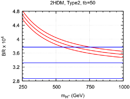
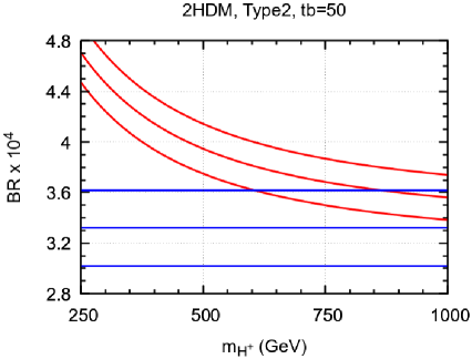
Figure 1: BR($B\to X_{s}\gamma$) as a function of the charged scalar mass. Left panel: The lines in blue represent the 3$\sigma$ experimental limits, and those in red to 2.5% error in the calculation. Right panel: The lines in blue represent the 2$\sigma$ experimental limits, and those in red to 5% error in the calculation.

On the left panel we considered a band corresponding to 2.5% in the calculation and a 3$\sigma$ band for the experimental result. On the right panel we considered a band corresponding to 5% in the calculation and a 2$\sigma$ band for the experimental result. We see that the limit for the mass of the charged scalar that we get is similar in both cases and also similar to what was obtained in ref. Misiak:2017bgg

As we are not doing a NNLO calculation, our goal here is not to improve the limit for the 2HDM with type 2 couplings. We just want to show that in models with more charged scalars, as was addressed in ref. Akeroyd:2020nfj , the limit in eq. (58) can be relaxed for one of them and this will have implications for the Zee model. We discuss this in the next section for the case of the Zee model. For definiteness we take the choice on the left panel of fig. 1.

IV.3.3 Implications for the Zee Model

We have just seen that in the case of having just one charged scalar boson we have a limit for its mass coming from the BR($B\to X_{s}\gamma$) for the case of 2HDM with type 2 fermion couplings. Now we consider the case of the Zee model also with type 2 fermion couplings. We start by just considering the variation of the masses and of the mixing angle $\gamma$ without imposing all the theoretical and experimental constraints on the model. That will be done below when we consider the discussion of benchmark points. Our purpose here is just to show how the constraints from BR($B\to X_{s}\gamma$) can be satisfied in the model. Although we can always choose $m_{H_{1}^{+}}<m_{H_{2}^{+}}$, we start by not imposing that constraint. All points satisfying eq. (61) are shown on the left panel of fig. 2.

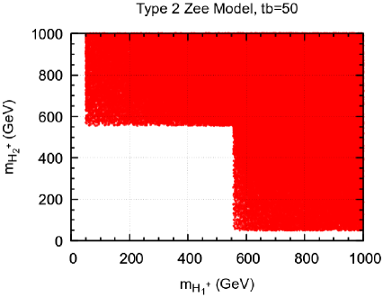
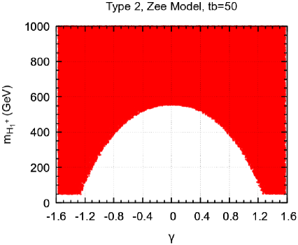
Figure 2: Left panel: points satisfying eq. (61) for the Zee Model. Right panel: mass of the lightest charged scalar boson as a function of the mixing angle $\gamma$.

We see that we have an exclusion for both masses to be below the value found (in the 2HDM) with one single charged scalar, but it is possible that one of the masses is lower than 580 GeV if the other is above. This is a function of the mixing angle $\gamma$ as shown on the right panel of fig. 2. We see that $m_{H_{1}^{+}}$ can be as low as 50 GeV if the mixing angle is close to $\pm\pi/2$. Notice that for $\gamma=0$ we recover the previous result. As can be seen from fig. 2, when $m_{H_{1}^{+}}$ is low, the other mass has always to be above the 580 GeV limit.

This result means that for each point in parameter space we have to evaluate the BR($B\to X_{s}\gamma$) to see if it passes the bounds in eq. (61), instead of using just one fixed limit for all points, like in the 2HDM.

Notice that in the Zee model there is no exact cancelation of the two charge scalar contributions. This is due to the fact that there is only one charge scalar component coming from a doublet, as we have explained after eq. (39). In contrast, in a 3HDM the charged scalars originate in two components of doublets and such a cancelation is indeed possible Boto:2021 .

There is a final comment. The charged Higgs contribute to $\Delta M_{B_{s,d}}$, coming from the B meson oscillations. We have not considered this contribution from flavour data because, as shown in Chakraborti:2021bpy , they are important only for very low $\tan\beta$, above what we get from the other constraints; see fig. 3 below.

IV.4 Scanning strategy

We made our scans varying the parameters in the following ranges,

$$m_{h_{1}}=125\,\text{GeV}, m_{h_{2}},m_{h_{3}},m_{H_{1}^{+}}\in[100,1000]\text{GeV}, m_{H_{2}^{+}}\in[500,1000]\text{GeV},$$ (66)

$$\alpha\in[-\frac{\pi}{2},\frac{\pi}{2}], \tan\beta\in[0,60], \gamma\in[-\frac{\pi}{2},\frac{\pi}{2}],$$ (67)

$$m_{12}^{2}\in[10^{-1},10^{6}]\text{GeV}^{2}, \lambda_{c}\in[10^{-3},10^{2}], k_{{}_{1}}\in[10^{-3},10^{2}],$$ (68)

$$k_{{}_{2}}\in[10^{-3},10^{2}], k_{{}_{12}}\in[10^{-3},10^{2}],$$ (69)

and take randomly $m^{2}_{12},k_{{}_{12}}$ with both signs. Despite this flat scan, there are large correlations in the points that satisfy all the constraints. For instance, we show in fig. 3 the correlation between $\alpha$ and $\beta$. We see that all the points satisfy $|\cos(\beta-\alpha)|\lesssim 1$, that is they are close to the alignment limit, where the 125GeV neutral scalar has couplings equal to their SM values. The points with negative $\alpha$ correspond to the wrong sign of the fermion couplings Ferreira:2014naa ; Fontes:2014tga . We also see that despite having varied $\tan\beta$ in a larger interval, the good points have $\tan\beta\in[1,10]$.

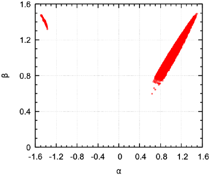
Figure 3: Left panel: correlation between $\alpha$ and $\beta$; Right panel: correlation between $\alpha$ and $\tan\beta$.

V Impact of the charged scalars on the decays $h\to\gamma\gamma$ and $h\to Z\gamma$

V.1 The diagrams of the charged scalars

As we discussed before, the distinctive feature of our implementation of the Zee model is the appearance of the off-diagonal coupling $ZH_{1}^{\pm}H_{2}^{\mp}$. This contributes to the loop decay $h\to Z\gamma$ and, in principle, could lead to some new feature. For the decay $h\to\gamma\gamma$, on the contrary, because of the photon coupling being always diagonal, the contribution of the charged scalars will not depend on the off-diagonal $ZH_{1}^{\pm}H_{2}^{\mp}$ coupling. In fact, the diagrams coming from the charged scalars and contributing in this model for $h\to\gamma\gamma$ are shown in fig. 4

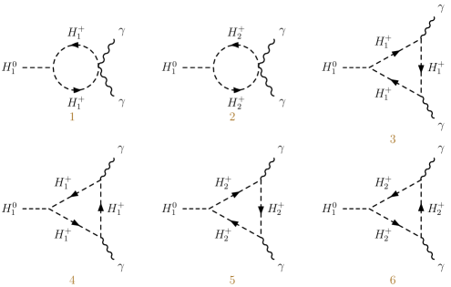
Figure 4: Charged scalars contributions to $h\to\gamma\gamma$

while for the case of the decay $h\to Z\gamma$, besides those equivalent to fig. 4 (with one $\gamma$ exchanged with a $Z$) we also have those with the off-diagonal coupling, as shown in fig. 5.

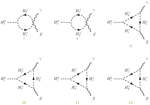
Figure 5: Extra charged scalars contributions to $h\to Z\gamma$

The formulas for these loop decays in the absence of couplings of the type $ZH_{1}^{+}H_{2}^{+}$ are well known. They were explicitly written for the C2HDM in ref. Fontes:2014xva and, for $h\to\gamma\gamma$, they can be easily adapted for the case of the Zee model. We generalize the formulas for $h\to Z\gamma$ to include the new couplings, and write the full expressions in appendix B. The new couplings needed are given in appendix A and were obtained with the help of the software FeynMasterFontes:2019wqh , that uses QGRAFnogueira:1991ex , FeynRuleschristensen:2008py ; Alloul:2013bka and FeynCalcMertig:1990an ; Shtabovenko:2016sxi in an integrated way.

V.2 Discussion of the impact of the charged scalars on the loop decays

V.2.1 Couplings $h_{1}H^{+}_{j}H^{-}_{k}$

The couplings $h_{1}H^{+}_{1}H^{-}_{1}$ and $h_{1}H^{+}_{2}H^{-}_{2}$ do not have a strong dependence on $\gamma$. On the contrary the couplings $h_{1}H^{+}_{1}H^{-}_{2}$ and $h_{1}H^{+}_{2}H^{-}_{1}$ are proportional to $\sin\gamma$.

V.2.2 Couplings $ZH^{+}_{j}H^{-}_{k}$

The couplings $ZH^{+}_{1}H^{-}_{2}$ and $ZH^{+}_{2}H^{-}_{1}$ are given in eqs. (86b)-(86c). They are proportional to $\sin(2\gamma)$ and vanish for $\gamma=0,\pm\pi/2$, while the couplings $ZH^{+}_{1}H^{-}_{1}$ and $ZH^{+}_{2}H^{-}_{2}$ vary with $\gamma$ like

$$g_{ZH^{+}_{i}H^{-}_{i}}\propto(-1+4s_{W}^{2}+\cos 2\gamma)\,.$$ (70)

It is interesting to note that because $-1+4s_{W}^{2}\simeq 0$ they behave approximately like $\cos 2\gamma$ that vanishes at $\pm\pi/4$.

V.2.3 Results and Conclusions

Because of the dependence of the couplings on the mixing angle $\gamma$, we looked at the contributions of the charged scalars as a function of this angle. If the loop integral did not vary much with the masses, the results would be proportional to the products of the $h_{1}H_{j}^{+}H_{k}^{-}$ and $ZH_{j}^{+}H_{k}^{-}$ couplings, as the photon coupling is universal. In the following figures all points passed all the constraints, including HiggsBounds 5.9.0 and those coming from BR($B\to X_{s}\gamma$), as discussed in section IV.3.

In fig. 6 we show on the left panel the result of the product of the couplings (we divide by $v$ because the coupling $h_{1}H_{j}^{+}H_{k}^{-}$ has dimensions of mass), first for the the case of $H_{1}^{+}$ running in the loops of fig. 4 in red and then for the case of $H_{2}^{+}$ in blue. From the above discussion we expect the result to vary like $\cos 2\gamma$, and that is indeed the case. Our assumptions that the loop integrals do not depend much on the masses can be verified in the right panel of fig. 6 where we show the actual plot for the loop amplitudes. The behaviour as $\cos 2\gamma$ is clear in both cases.

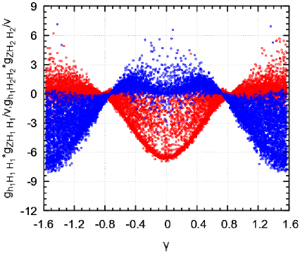
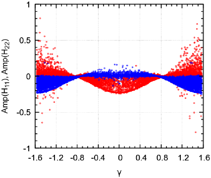
Figure 6: Results for the charged scalars amplitudes contribution to $h\to Z\gamma$. On the left panel the coupling products and on the right panel the actual amplitudes.

Now we can study the case where there are two different charged scalars, $H_{1}^{+}$ and $H_{2}^{+}$, running in the loops of fig. 5. This is shown in fig. 7.

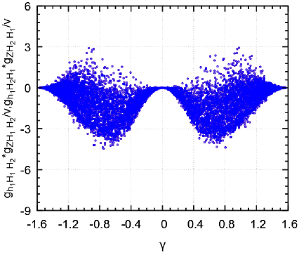
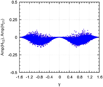
Figure 7: Results for the charged scalars amplitudes contribution to $h\to Z\gamma$. On the left panel the coupling products and on the right panel the actual amplitudes.

Again on the left panel we plot the product of the couplings, and on the right panel the loop amplitudes. In this case Amp($H_{1}^{+},H_{2}^{+}$), corresponding to diagrams 7, 10 and 11 of fig. 5 in red, coincides with Amp($H_{2}^{+},H_{1}^{+}$) corresponding to diagrams 8, 9 and 12. As expected we see clearly a dependence on $\sin 2\gamma$, confirming our expectations.

However this nice result will not help us in using the decay $h\to Z\gamma$ to identify the novel coupling $ZH_{1}^{+}H_{2}^{-}$ appearing in the Zee model. The problem is that once we sum all contributions we loose the dependence on $\gamma$. This can be seen on fig. 8 both for the products of the couplings in the left panel, and for the final result for the charged scalar contribution to $h\to Z\gamma$.

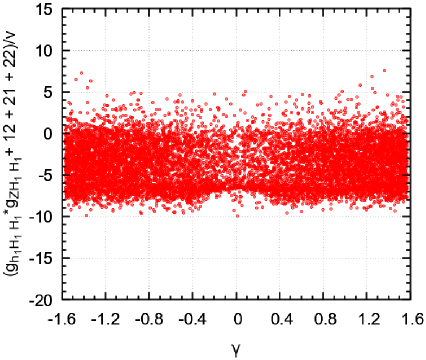
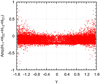
Figure 8: Results for the charged scalar amplitudes contribution to $h\to Z\gamma$. On the left panel the sum of the product of couplings and on the right panel the complete result.

In conclusion, although the contribution of the charged scalars can have both signs and also be zero, the dependence on $\gamma$ and therefore on the mixing parameters $\mu_{4}$ is hidden. In fact we can have the same behaviour of the charged scalar amplitudes in other models like the 3HDM Boto:2021 .

VI Decays of the Charged Higgs

VI.1 The decay $H_{2}^{+}\to H_{1}^{+}+Z$

If we want to have a unique signal for this model it would be the decay of one charged Higgs in another one plus a $Z$ boson. This is only possible if $\gamma\not=0$. We have checked that this can indeed occur, as shown in fig. 9. All points shown satisfy all the constraints discussed in section IV.

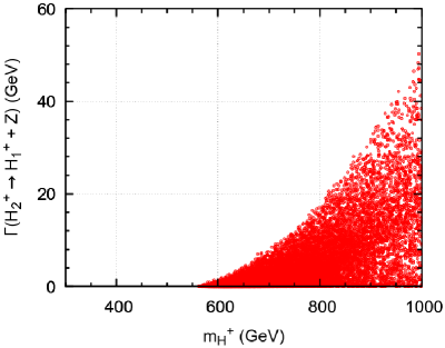
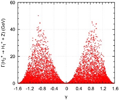
Figure 9: Decay with $H_{2}^{+}\to H_{1}^{+}+Z$. On the left panel the dependence on the mass of the decaying charged Higgs and on the right the dependence on $\gamma$.

We see clearly that, as expected, one has to be away from $\gamma=0$ to have a sizable decay width.

VI.1.1 Decays of the heavier $H_{2}^{\pm}$

Depending on the masses the following decays are among the most important,

$$H_{2}^{\pm}\to H_{1}^{\pm}+Z\,, H_{2}^{+}\to t+\overline{b}\,, H_{2}^{\pm}\to H_{1}^{\pm}+h_{i}\,,$$ (71)

$$H_{2}^{\pm}\to W^{\pm}+h_{i}\,, H_{2}^{+}\to\nu_{\tau}+\tau^{+}\,.$$ (72)

The first decay is unique to this type of models and not present in NHDM. It requires a mixing between the charged Higgs from the doublets with the charged Higgs from the singlets. The expression for the width is

$$\Gamma(H_{2}^{\pm}\to H_{1}^{\pm}+Z)=\frac{g^{2}}{64\pi m_{H^{+}_{j}}^{3}M_{W}^{2}}\,g_{\rm HpjHmkZ}[2,1]^{2}\,\lambda(m_{H^{+}_{2}}^{2},m_{H^{+}_{1}}^{2},M_{Z}^{2})^{3},$$ (73)

where the Källen function is given by

$$\lambda(x^{2},y^{2},z^{2})=\sqrt{x^{4}+y^{4}+z^{4}-2x^{2}y^{2}-2x^{2}z^{2}-2y^{2}z^{2}}.$$ (74)

For the other decays we have

$$\Gamma(H_{2}^{+}\to t+\overline{b})= \frac{3g^{2}}{32\pi M_{W}^{2}}m_{H_{2}^{+}}\lambda(m_{H_{2}^{+}},m_{t}^{2},m_{b}^{2})\left[(1-x_{t}-x_{b})(Y_{2}^{2}x_{t}+X_{2}^{2}x_{b})-4x_{t}x_{b}X_{2}Y_{2}\right],$$ (75)

where

$$x_{t}=\frac{m_{t}^{2}}{m_{H_{2}^{+}}},\quad x_{b}=\frac{m_{b}^{2}}{m_{H_{2}^{+}}},$$ (76)

and $X_{k},Y_{k}$ are given in eq. (91a). For the decay into the other charged Higgs and one neutral Higgs boson we have,

$$\Gamma(H_{2}^{\pm}\to H_{1}^{\pm}+h_{i})= \frac{g_{\rm hjHpiHmk}[i,2,1]^{2}}{16\pi m_{H^{+}_{2}}^{3}}\lambda(m_{H_{2}^{+}},m_{H_{1}^{+}},m_{h_{i}}^{2}).$$ (77)

The decay into one W and one neutral Higgs boson is similar to the decay into the charged Higgs and Z. We obtain

$$\Gamma(H_{2}^{\pm}\to W^{\pm}+h_{i})= \frac{g^{2}}{64\pi m_{H^{+}_{2}}^{3}M_{W}^{2}}\,g_{\rm hjHpkWm}[i,2]^{2}\,\lambda(m_{H^{+}_{2}}^{2},M_{W}^{2},m_{h_{i}}^{2})^{3}.$$ (78)

Finally the decay in the third family leptons (the others are negligible) is given by

$$\Gamma(H_{2}^{+}\to\nu_{\tau}+\tau^{+})= \frac{g^{2}}{32\pi M_{W}^{2}}\,Z_{2}^{2}\,m_{\tau}^{2}\,m_{H^{+}_{2}}\left[1-\frac{m_{\tau}^{2}}{m_{H^{+}_{2}}^{2}}\right]^{2}.$$ (79)

VI.1.2 Decays of the lighter $H_{1}^{\pm}$

Except for the decays into another charged Higgs, that are not allowed because we assume that $m_{H_{1}^{+}}<m_{H_{2}^{+}}$, the decays are similar to those of the heavier charged scalar. If kinematically available, the expressions for the decays can be easily obtained from the above with index $2\to 1$. All the couplings needed are given in appendix A and were obtained with the help of the software FeynMasterFontes:2019wqh .

VII Benchmark points for the Zee model

VII.1 Looking for a distinctive signature

As we have discussed before, the Zee model provides an example of the non-vanishing coupling between two different charged Higgs and the Z boson. For instance, this cannot happen in any NHDM, even with a large N. So we want to see if there is a signal of this coupling.

As we explained in section V, the first idea was to look at the impact on the BR($h_{125}\to Z\gamma$). But it turns out that the effect of the extra diagrams is not quantitatively different from the effect of a second charged scalar coupling only diagonally to the $Z$ boson, as occurs for instance in the 3HDM, where there are two charged Higgs bosons, but no $ZH_{1}^{+}H_{2}^{-}$ coupling Boto:2021 . So, although there is an effect, for instance the contribution of summing over all the charged Higgs diagrams can vanish, this is not an effect specific to the $ZH_{1}^{+}H_{2}^{-}$ coupling. So we turn to a distinctive decay:

$$H_{2}^{+}\to H_{1}^{+}+Z,\quad\text{and}\quad H_{1}^{+}\to t+\overline{b}$$ (80)

This decay has a very clear signature and should be searched for at the LHC.

VII.2 Benchmark Point $P_{1}$

As the model has many independent parameters, if we try to plot the various branching ratios of the $H_{1}^{+}$ or $H_{2}^{+}$ instead of obtaining something similar to the famous plot Djouadi:2005gi of the SM Higgs boson BR’s as a function of its mass (when this mass was yet not known), we would get a figure with all the points superimposed and no lines. So, to have a better visualization we fix most of the parameters and show that indeed the branching ratios for the processes in eq. (80) can be important, or even dominant. This leads us to the choice of benchmark points. In choosing these benchmark points for the Zee model we take in account all the theoretical and experimental constraints on the model.

For the first benchmark point, $P_{1}$, we choose a situation when both masses are above the limit of eq. (58). It is defined by the following parameters,

$$m_{h_{1}}=125\,\text{GeV} m_{h_{2}}=714.98\,\text{GeV} m_{h_{3}}=767.42\,\text{GeV}$$ (81a)

$$m_{H_{1}^{+}}=m_{H_{2}^{+}}-200\,\text{GeV} \alpha=1.391 \gamma=0.894$$ (81b)

$$m_{12}^{2}=8.828\times 10^{4}\,\text{GeV}^{2} \lambda_{c}=0.4363 k_{{}_{1}}=0.4633$$ (81c)

$$k_{{}_{2}}=0.4633 k_{{}_{12}}=5.427\times 10^{-2}$$ (81d)

The situation is shown in fig. 10.

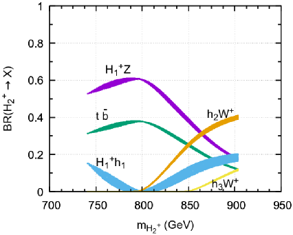
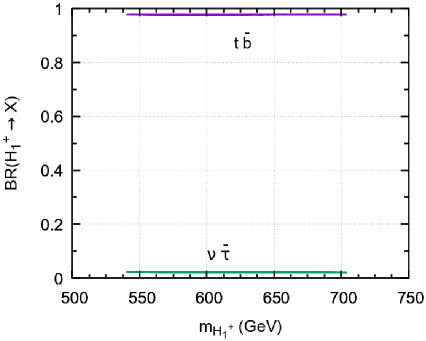
Figure 10: Dominant BR’s for $H_{2}^{+}$ (left panel) and $H_{1}^{+}$ (right panel) for benchmark point $P_{1}$.

We see that our signal decay has the largest branching ratio, while $H_{1}^{+}$ decays almost 100% into $t+\overline{b}$. This should provide clear signatures at the LHC. A detailed analysis, with background studies, should of course be done. The width of the bands comes from the variation of $\tan\beta$ (at the percent level, because the good points have $\alpha\simeq\beta$). All the points pass all the constraints, including that of eq. (61).

VII.3 Benchmark Point $P_{2}$

One could argue that $P_{1}$ will lead to a situation where the constraint of eq. (61) was verified, as we took the masses to satisfy the bound of eq. (58). Therefore we want to show another benchmark point that would be excluded by eq. (58). That is, we do not exclude points a priori, but for each point we evaluate the BR($B\to X_{s}\gamma$) to see if it passes the bounds in eq. (61).

For the second benchmark point $P_{2}$ we therefore choose a situation where the lowest charged Higgs mass is below that limit. It is defined by the following parameters

$$m_{h_{1}}=125\,\text{GeV} m_{h_{2}}=580.7\,\text{GeV} m_{h_{3}}=633.7\,\text{GeV}$$ (82a)

$$m_{H_{1}^{+}},m_{H_{2}^{+}}\text{GeV},\ \text{scanned as shown} \alpha=1.398 \gamma=1.089$$ (82b)

$$m_{12}^{2}=5.77\times 10^{4}\,\text{GeV}^{2} \lambda_{c}=4.473 k_{{}_{1}}=1.082$$ (82c)

$$k_{{}_{2}}=3.98\times 10^{-3} k_{{}_{12}}=-1.266\times 10^{-3}$$ (82d)

The situation is shown in fig. 11.

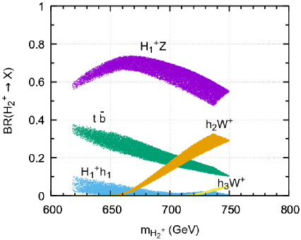
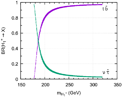
Figure 11: Dominant BR’s for $H_{2}^{+}$ (left panel) and $H_{1}^{+}$ (right panel) for benchmark point $P_{2}$.

We see that our signal decay has the largest branching ratio, while $H_{1}^{+}$ decays almost 100% into $t+\overline{b}$. This should be clear signatures at the LHC, although background studies should be done. The width of the bands comes from the variation of $\tan\beta$ and $m_{H_{1}^{+}},m_{H_{2}^{+}}$ which were varied independently. All the points pass all the constraints, including that of eq. (61).

VII.4 Benchmark Point $P_{3}$

We have a large set of benchmark points that illustrate our signal, the decay $H_{2}^{+}\to H_{1}^{+}+Z$. We just give another example, our benchmark point $P_{3}$. It is defined by the following parameters,

$$m_{h_{1}}=125\,\text{GeV} m_{h_{2}}=728.3\,\text{GeV} m_{h_{3}}=720.5\,\text{GeV}$$ (83a)

$$m_{H_{1}^{+}},m_{H_{2}^{+}}\text{GeV},\ \text{scanned as shown} \alpha=1.401 \gamma=-1.145$$ (83b)

$$m_{12}^{2}=9.48\times 10^{4}\,\text{GeV}^{2} \lambda_{c}=2.67\times 10^{-2} k_{{}_{1}}=7.149$$ (83c)

$$k_{{}_{2}}=1.425\times 10^{-2} k_{{}_{12}}=1.29\times 10^{-2}$$ (83d)

The situation is shown in fig. 12.

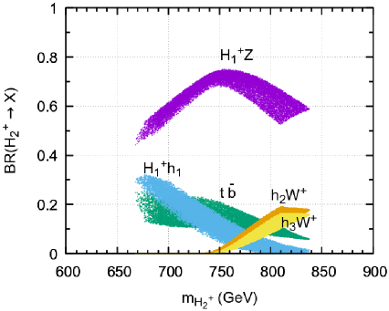
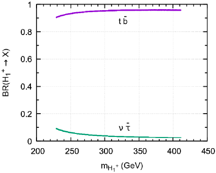
Figure 12: Dominant BR’s for $H_{2}^{+}$ (left panel) and $H_{1}^{+}$ (right panel) for benchmark point $P_{3}$.

Again we see that our signal decay has the largest branching ratio, while $H_{1}^{+}$ decays almost 100% into $t+\overline{b}$. The width of the bands comes from the variation of $\tan\beta$ and $m_{H_{1}^{+}},m_{H_{2}^{+}}$ which were varied independently. All the points pass all the constraints, including that of eq. (61).

VII.5 Benchmark Point $P_{4}$

It has been pointed out recently Bahl:2021str , that there are some decay channels for the charged Higgs that have not been investigated at LHC. One of them is the decay $H_{1}^{+}\to W^{+}+h_{1}$. We looked in our data sample for points where the BR$(H_{1}^{+}\to W^{+}+h_{1})$ could be large. For our model, after passing through the HiggsBounds 5, there are not many points of the general scan that have a large BR$(H_{1}^{+}\to W^{+}+h_{1})$. We took one of these which is our benchmark point $P_{4}$. It is defined by the following parameters,

$$m_{h_{1}}=125\,\text{GeV} m_{h_{2}}=314.9\,\text{GeV} m_{h_{3}}=651.3\,\text{GeV}$$ (84a)

$$m_{H_{1}^{+}},m_{H_{2}^{+}}\,\text{GeV},\text{scanned as shown} \alpha=-1.402 \gamma=-1.421$$ (84b)

$$m_{12}^{2}=1.85\times 10^{4}\,\text{GeV}^{2} \lambda_{c}=2.00\times 10^{-2} k_{{}_{1}}=1.422\times 10^{-2}$$ (84c)

$$k_{{}_{2}}=0.432 k_{{}_{12}}=-9.597\times 10^{-3}$$ (84d)

The situation is shown in fig. 13.

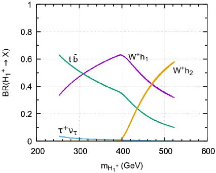
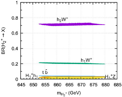
Figure 13: Dominant BR’s for $H_{1}^{+}$ (left panel) and $H_{2}^{+}$ (right panel) for benchmark point $P_{4}$.

We see that, in our model, both BR$(H_{1}^{+}\to W^{+}+h_{1})$ and BR$(H_{1}^{+}\to W^{+}+h_{2})$ can be sizable. In this case, the BR$(H_{2}^{+}\to H_{1}^{+}+Z)$ is very small, around 2%. However the BR$(H_{2}^{+}\to W^{+}+h_{1})$ and BR$(H_{2}^{+}\to W^{+}+h_{2})$ can also be large, making this an interesting benchmark point. The width of the bands comes from the variation of $\tan\beta$, $m_{H_{1}^{+}}$, and $m_{H_{2}^{+}}$, which were varied independently. All the points pass all the constraints, including that of eq. (61).

VII.6 Production cross-sections and Experimental bounds

One can ask if a charged Higgs boson with a large BR($H^{+}\to t\overline{b}$) is not in contradiction with experimental bounds from the LHC. Although we have checked all the points with HiggsBounds 5.9.0 Bechtle:2020pkv , it is perhaps helpful to show it explicitly for our benchmark points. The results are shown in fig. 14 and fig. 15.

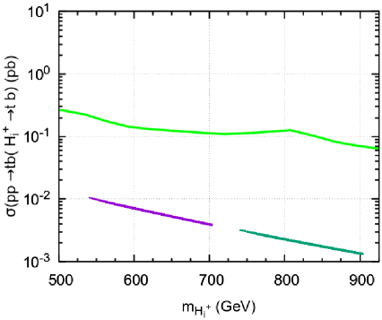
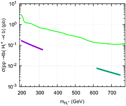
Figure 14: $\sigma(pp\to tbH^{+})\times BR(H^{+}\to tb)$ versus the charged Higgs mass for benchmark points $P_{1}$ (left panel) and $P_{2}$ (right panel). We took BR($H^{+}\to tb$)$=1$. The green line is the current LHC limit.

We used the values for the production cross-section $\sigma(pp\to tbH^{+})$ from ref. Degrande:2015xnm ; Degrande:2016hyf .

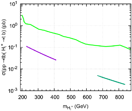
Figure 15: $\sigma(pp\to tbH^{+})\times BR(H^{+}\to tb)$ versus the charged Higgs mass for benchmark points $P_{1}$ (left panel) and $P_{2}$ (right panel). We took BR($H^{+}\to tb$)$=1$. The green line is the current LHC limit.

To see if the points are allowed we considered the worst case scenario where BR($H^{+}\to tb$)=1 (although for our benchmark points this is only true for the lightest charged Higgs boson); see fig. 7 and fig. 8. The green line is the current experimental bound from ATLAS ATLAS:2020jqj as discussed in ref. Bahl:2021str . So we conclude that all our benchmark points are consistent with the latest LHC data.

VIII Conclusions

A singular feature of models with multiple scalar doublets and charged singlets is the presence of off-diagonal $ZH_{1}^{\pm}H_{2}^{\mp}$ couplings. We have studied this feature in detail, using the scalar sector of the Zee model as an example.

Some formulae are presented in a form useful for generic models with any number of doublet and singlet scalars. We use in our scans all known theoretical constraints, including a careful analysis of the BFB conditions, the exclusion of lower-lying CB vacua, and the unitarity conditions derived here for this model.

We show that $ZH_{1}^{\pm}H_{2}^{\mp}$ couplings appear in $h\rightarrow Z\gamma$ and $B\rightarrow X_{s}\gamma$, but that there they do not impose features beyond those already present in generic 3HDM (where such off-diagonal couplings are not present).

We stress the importance of looking experimentally for $H_{2}^{+}\rightarrow H_{1}^{+}Z$ decays and propose interesting benchmark points. We also found in our model interesting values for the decays recently proposed in Bahl:2021str . We found that there are regions of parameter space consistent with large branching ratios for $H_{1}^{+}\rightarrow W^{+}h_{1,2}$ or $H_{2}^{+}\rightarrow W^{+}h_{1,2}$. But, in those cases, we found no case where simultaneously BR($H_{2}^{+}\rightarrow H_{1}^{+}Z$) was large. We strongly urge a search for $H_{2}^{+}\rightarrow H_{1}^{+}Z$ decays.

Appendix A Couplings of the charged Higgs

A.1 Couplings to the Z boson

We define the coupling as

$$[H^{+}_{j},H^{-}_{k},Z]:=-i\ \frac{g}{2c_{W}}(p_{H_{j}^{+}}-p_{H_{k}^{-}})^{\mu}g_{\rm HpjHmkZ}[j,k],$$ (85)

where all particles are entering the vertex and

$$g_{\rm HpjHmkZ}[1,1]= \frac{1}{2}\left(c_{W}^{2}-3s_{W}^{2}+\cos(2\gamma)\right),$$ (86a)

$$g_{\rm HpjHmkZ}[1,2]= -\frac{1}{2}\sin(2\gamma),$$ (86b)

$$g_{\rm HpjHmkZ}[2,1]= -\frac{1}{2}\sin(2\gamma),$$ (86c)

$$g_{\rm HpjHmkZ}[2,2]= \frac{1}{2}\left(c_{W}^{2}-3s_{W}^{2}-\cos(2\gamma)\right),$$ (86d)

Notice that when the mixing angle $\gamma$ vanishes the singlet decouples from the doublet and there is no $[H^{+}_{j},H^{-}_{k},Z]$ vertex for $j\not=k$.

A.2 Couplings to the W boson

For CP even neutral Higgs bosons ($j=1,2$) we define the coupling as

$$[h_{j},H^{+}_{k},W^{-}]:-i\,\frac{g}{2}(p_{H^{+}_{k}}-p_{h_{j}})^{\mu}g_{\rm hjHpkWm}[j,k],$$ (87)

where all particles are entering the vertex. For CP odd neutral Higgs boson ($j=3$) we define

$$[h_{3},H^{+}_{k},W^{-}]:=\frac{g}{2}(p_{h_{3}}-p_{H^{+}_{k}})^{\mu}g_{\rm hjHpkWm}[3,k],$$ (88)

where

$$g_{\rm hjHpkWM}[1,1]= \cos(\gamma)\sin(\alpha-\beta)),$$ (89a)

$$g_{\rm hjHpkWM}[1,2]= -\sin(\alpha-\beta)\sin(\gamma),$$ (89b)

$$g_{\rm hjHpkWM}[2,1]= \cos(\alpha-\beta)\cos(\gamma),$$ (89c)

$$g_{\rm hjHpkWM}[2,2]= -\cos(\alpha-\beta)\sin(\gamma),$$ (89d)

$$g_{\rm hjHpkWM}[3,1]= \cos(\gamma),$$ (89e)

$$g_{\rm hjHpkWM}[3,2]= -\sin(\gamma),$$ (89f)

A.3 Couplings to quarks and leptons

The interactions of charged Higgs bosons with quarks are given by the following Lagrangian

$$\mathcal{L}=\frac{g}{\sqrt{2}}\left[\frac{m_{d_{j}}}{M_{W}}X_{k}\overline{u}_{i}V_{ij}P_{R}d_{j}+\frac{m_{u_{i}}}{M_{W}}X_{k}\overline{u}_{i}V_{ij}Y_{k}P_{L}d_{j}+\frac{m_{l}}{M_{W}}Z_{k}\overline{\nu}_{l}P_{R}e_{l}\right]H_{k}^{+}+\text{h.c.}$$ (90)

where $k=1,2$ and we have used the conventions of Borzumati and Greub Borzumati:1998tg , extended in ref. Akeroyd:2020nfj , which is convenient for the BR($B\to X_{s}\gamma$) calculation. We get

$$X_{1}= \tan\beta\cos\gamma, Y_{1}=\cot\beta\cos\gamma, Z_{1}=\tan\beta\cos\gamma,$$ (91a)

$$X_{2}= -\tan\beta\sin\gamma, Y_{2}=-\cot\beta\sin\gamma, Z_{2}=-\tan\beta\sin\gamma,$$ (91b)

A.4 Couplings to neutral Higgs

Finally the couplings to the neutral Higgs are given by the Lagrangian

$$\mathcal{L}=H^{+}_{i}H^{-}_{k}h_{j}g_{\rm hjHpiHmk}[j,i,k],$$ (92)

where $g_{\rm hjHpiHmk}$ are long expressions that we do not reproduce here. Note however that $g_{\rm hjHpiHmk}(3,i,k)=0$.

Appendix B The decays $h\rightarrow\gamma\gamma$ and $h\rightarrow Z\gamma$

These decays were calculated for the 2HDM to one loop approximation in Fontes:2014xva . Since most terms in the Lagrangian of our model only differ by multiplicative constants, our results will only change by some factors. We adapt from Fontes:2014xva for the next results. The major difference occurs in $h\rightarrow Z\gamma$, where the presence of the $ZH_{1}^{\pm}H_{2}^{\mp}$ coupling allows for the new diagrams in fig. 5.

B.1 Fermion Loops

The fermion loops are easily obtained plugging the couplings of eq. (14) in the results of Fontes:2014xva :

$$X_{F}^{\gamma\gamma} =-\sum_{f}N_{c}^{f}2a_{f}^{2}Q_{f}^{2}\tau_{f}[1+(1-\tau_{f})f(\tau_{f})]\,,$$

$$Y_{F}^{\gamma\gamma} =-\sum_{f}N_{c}^{f}2b_{f}^{2}Q_{f}^{2}\tau_{f}f(\tau_{f})\,,$$

$$X_{F}^{Z\gamma} =-\sum_{f}N_{c}^{f}\frac{4a_{f}^{2}g_{V}^{f}Q_{f}m_{f}^{2}}{s_{W}c_{W}}\Bigg{[}\frac{2M_{Z}^{2}}{(m_{h}^{2}-M_{Z}^{2})^{2}}\left[B_{0}(m_{h}^{2},m_{f}^{2},m_{f}^{2})-B_{0}(M_{Z}^{2},m_{f}^{2},m_{f}^{2})\right]$$ (93)

$$+\frac{1}{m_{h}^{2}-M_{Z}^{2}}\left[(4m_{f}^{2}-m_{h}^{2}+M_{Z}^{2})C_{0}(M_{Z}^{2},0,m_{h}^{2},m_{f}^{2},m_{f}^{2},m_{f}^{2})+2\right]\Bigg{]}\,,$$

$$Y_{F}^{Z\gamma} =-\sum_{f}N_{c}^{f}\frac{4b_{f}^{2}g_{V}^{f}Q_{f}m_{f}^{2}}{s_{W}c_{W}}C_{0}(M_{Z}^{2},0,m_{h}^{2},m_{f}^{2},m_{f}^{2},m_{f}^{2})\,,$$

where $N_{c}^{f}$ is 3 for quarks and 1 for leptons, $Q_{f}$ is the fermion charge, $g_{V}^{f}$ is the fermion’s vector coupling to the $Z$ boson and the sums run over all fermions $f$. The function appearing is defined as

$$f(\tau)=-\frac{2m_{f}^{2}}{\tau_{f}}C_{0}(0,0,m_{h}^{2},m_{f}^{2},m_{f}^{2},m_{f}^{2})=\left\{\begin{array}[]{ll}\left[\sin^{-1}\left(\sqrt{1/\tau}\right)\right]^{2},&\ \ \text{if}\ \tau\geq 1\\[5.69054pt] -\frac{1}{4}\left[\displaystyle\ln\left(\frac{1+\sqrt{1-\tau}}{1-\sqrt{1-\tau}}\right)-i\pi\right]^{2},&\ \ \text{if}\ \tau<1\end{array}\right.\,,$$ (94)

while $B_{0}$ and $C_{0}$ are the Passarino-Veltman functions.

B.2 Charged gauge boson loops

The only change in these loops comes from the $hVV$ vertex, which is multiplied by a factor $\text{Re}(\omega^{\dagger}V)^{\beta}$, and so is the loop. Using the notation of Fontes:2014xva , we have

$$X_{W}^{\gamma\gamma} =\text{Re}(\omega^{\dagger}V)^{\beta}\left[2+3\tau_{W}+3\tau_{W}(2-\tau_{W})f(\tau_{W})\right]\,,$$

$$X_{W}^{Z\gamma} =\frac{\text{Re}(\omega^{\dagger}V)^{\beta}}{\tan\theta_{W}}I_{W}\,,$$ (95)

where,

$$\omega_{a} =v_{a}/v,\;\;\;\tau_{W}=\frac{4M_{W}^{2}}{m_{h}^{2}}\,,$$

$$I_{W} =\frac{1}{(m_{h}^{2}-M_{Z}^{2})^{2}}\left[m_{h}^{2}(1-\tan^{2}\theta_{W})-2M_{W}^{2}(-5+\tan^{2}\theta_{W})\right]M_{Z}^{2}\Delta B_{0}\,,$$

$$+\frac{1}{m_{h}^{2}-M_{Z}^{2}}[m_{h}^{2}(1-\tan^{2}\theta_{W})-2M_{W}^{2}(-5+\tan^{2}\theta_{W})\,,$$ (96)

$$+2M_{W}^{2}\left[(-5+\tan^{2}\theta_{W})(m_{h}^{2}-2M_{W}^{2})-2M_{Z}^{2}(-3+\tan^{2}\theta_{W})]C_{0}\right]M_{Z}^{2}\Delta B_{0}\,,$$

$$\Delta B_{0} =B_{0}(m_{h}^{2},M_{W}^{2},M_{W}^{2})-B_{0}(M_{Z}^{2},M_{W}^{2},M_{W}^{2})\,,$$

$$C_{0} =C_{0}(M_{Z}^{2},0,m_{h}^{2},M_{W}^{2},M_{W}^{2},M_{W}^{2})\,.$$

B.3 Charged Scalar Loops

For the decay to $\gamma\gamma$, the loops are the same as the one presented in Fontes:2014xva with the cubic scalar vertex replaced by the ones we defined in eq. (7). Besides this replacement, we only need to sum over the charged scalars, obtaining

$$X_{H}^{\gamma\gamma}=-\sum_{\alpha}\frac{\lambda^{2\alpha\alpha}v^{2}}{2m_{\pm\alpha}^{2}}\tau_{\pm\alpha}[1-\tau_{\pm\alpha}f(\tau_{\pm\alpha})]\,,$$ (97)

where $\tau_{\pm\alpha}=4m_{h}^{2}/m_{\pm\alpha}$. Regarding the decay to $Z\gamma$, we can allow two different scalars to run within the same loop, as seen in fig. 5. This generalizes the result in Fontes:2014xva . We obtain

$$X_{H}^{Z\gamma} =-\sum_{\alpha_{1}\alpha_{2}}\frac{(2s_{W}^{2}\delta^{\alpha_{1}\alpha_{2}}-(U^{\dagger}U)^{\alpha_{2}\alpha_{1}})}{\sin\theta_{W}\cos\theta_{W}}\frac{g^{2\alpha_{1}\alpha_{2}}}{m_{h}^{2}-M_{Z}^{2}}\Bigg{[}\frac{M_{Z}^{2}}{m_{h}^{2}-M_{Z}^{2}}\left(B_{0}(m_{h}^{2},m_{\pm\alpha_{1}}^{2},m_{\pm\alpha_{2}}^{2})\right.$$

$$\hskip 28.45274pt\left.-B_{0}(M_{Z}^{2},m_{\pm\alpha_{1}}^{2},m_{\pm\alpha_{2}}^{2})\right)+1+m_{\pm\alpha_{1}}^{2}C_{0}(M_{Z}^{2},0,m_{h}^{2},m_{\pm\alpha_{1}}^{2},m_{\pm\alpha_{1}}^{2},m_{\pm\alpha_{2}}^{2})$$

$$\hskip 28.45274pt+m_{\pm\alpha_{2}}^{2}C_{0}(M_{Z}^{2},0,m_{h}^{2},m_{\pm\alpha_{2}}^{2},m_{\pm\alpha_{2}}^{2},m_{\pm\alpha_{1}}^{2})\Bigg{]}\,.$$ (98)

If there were no cubic terms in eq. (5) ($\mu_{4}^{abi}=0$), then $(U^{\dagger}U)^{\alpha_{2}\alpha_{1}}=\delta^{\alpha_{2}\alpha_{1}}$ and there would be no diagrams involving simultaneously two different charged scalars.

B.4 Final widths for loop decays

The final widths are given by

$$\Gamma(h\rightarrow\gamma\gamma) =\frac{G_{F}\alpha^{2}m_{h}^{2}}{128\sqrt{2}\pi^{3}}\left(|X_{F}^{\gamma\gamma}+X_{W}^{\gamma\gamma}+X_{H}^{\gamma\gamma}|^{2}+|Y_{F}^{\gamma\gamma}|^{2}\right)\,,$$

$$\Gamma(h\rightarrow Z\gamma) =\frac{G_{F}\alpha^{2}m_{h}^{2}}{64\sqrt{2}\pi^{3}}\left(1-\frac{M_{Z}^{2}}{m_{h}^{2}}\right)^{3}\left(|X_{F}^{Z\gamma}+X_{W}^{Z\gamma}+X_{H}^{Z\gamma}|^{2}+|Y_{F}^{Z\gamma}|^{2}\right)\,.$$ (99)

Appendix C Perturbative unitarity

We write here the scattering matrices for the various $(Q,Y)$ combinations and list all the eigenvalues at the end. This is presented here for the first time. We follow the notation of Bento:2017eti

C.1 $Q=2,Y=1$

For the combination of states $S^{++}_{\alpha}$ in eq. (54a) we have

$$M^{++}_{2}=\begin{bmatrix}\lambda_{1}&0&0&\lambda_{5}&0&0\\ 0&\lambda_{3}+\lambda_{4}&0&0&0&0\\ 0&0&k_{1}&0&-k_{12}&0\\ \lambda_{5}&0&0&\lambda_{2}&0&0\\ 0&0&-k_{12}&0&k_{2}&0\\ 0&0&0&0&0&2\lambda_{c}\\ \end{bmatrix}\,.$$ (100)

C.2 $Q=1,Y=1$

For the combination of states $S^{+}_{\alpha}$ in eq. (54b) we have

$$M^{+}_{2}=\begin{bmatrix}\lambda_{1}&0&0&\lambda_{5}&0&0\\ 0&\lambda_{3}&\lambda_{4}&0&0&0\\ 0&\lambda_{4}&\lambda_{3}&0&0&0\\ \lambda_{5}&0&0&\lambda_{2}&0&0\\ 0&0&0&0&k_{1}&-k_{12}\\ 0&0&0&0&-k_{12}&k_{2}\\ \end{bmatrix}\,.$$ (101)

C.3 $Q=1,Y=0$

For the combination of states $T^{+}_{\alpha}$ in eq. (54c) we have

$$M^{+}_{0}=\begin{bmatrix}\lambda_{1}&0&0&\lambda_{4}&0&0\\ 0&\lambda_{3}&\lambda_{5}&0&0&0\\ 0&\lambda_{5}&\lambda_{3}&0&0&0\\ \lambda_{4}&0&0&\lambda_{2}&0&0\\ 0&0&0&0&k_{1}&-k_{12}\\ 0&0&0&0&-k_{12}&k_{2}\\ \end{bmatrix}\,.$$ (102)

C.4 $Q=0,Y=1$

For the combination of states $S^{0}_{\alpha}$ in eq. (54d) we have

$$M^{0}_{2}=\begin{bmatrix}0&0&0\\ 0&0&0\\ 0&0&0\\ \end{bmatrix}\,.$$ (103)

C.5 $Q=0,Y=0$

For the combination of states $T^{0}_{\alpha}$ in eq. (54e) we have

$$M^{0}_{0}=\setcounter{MaxMatrixCols}{13}\begin{bmatrix}2\lambda_{1}&0&0&0&\lambda_{34}&0&0&0&k_{1}&\lambda_{1}&0&0&\lambda_{3}\\ 0&2\lambda_{5}&0&\lambda_{34}&0&0&0&0&-k_{12}&0&\lambda_{5}&\lambda_{4}&0\\ 0&0&0&0&0&0&k_{1}&-k_{12}&0&0&0&0&0\\ 0&\lambda_{34}&0&2\lambda_{5}&0&0&0&0&-k_{12}&0&\lambda_{4}&\lambda_{5}&0\\ \lambda_{34}&0&0&0&2\lambda_{2}&0&0&0&k_{2}&\lambda_{3}&0&0&\lambda_{2}\\ 0&0&0&0&0&0&-k_{12}&k_{2}&0&0&0&0&0\\ 0&0&k_{1}&0&0&-k_{12}&0&0&0&0&0&0&0\\ 0&0&-k_{12}&0&0&k_{2}&0&0&0&0&0&0&0\\ k_{1}&-k_{12}&0&-k_{12}&k_{2}&0&0&0&4\lambda_{c}&k_{1}&-k_{12}&-k_{12}&k_{2}\\ \lambda_{1}&0&0&0&\lambda_{3}&0&0&0&k_{1}&2\lambda_{1}&0&0&\lambda_{34}\\ 0&\lambda_{5}&0&\lambda_{4}&0&0&0&0&-k_{12}&0&2\lambda_{5}&\lambda_{34}&0\\ 0&\lambda_{4}&0&\lambda_{5}&0&0&0&0&-k_{12}&0&\lambda_{34}&2\lambda_{5}&0\\ \lambda_{3}&0&0&0&\lambda_{2}&0&0&0&k_{2}&\lambda_{34}&0&0&2\lambda_{2}\\ \end{bmatrix}\,,$$ (104)

where for simplicity we have defined

$$\lambda_{34}\equiv\lambda_{3}+\lambda_{4}\,.$$ (105)

C.6 The independent eigenvalues

We can obtain easily the eigenvalues for all the matrices except for $M^{0}_{0}$ in eq. (104) for which we have to solve numerically a fourth order polynomial. The list of independent eigenvalues is,

$$\Lambda_{1}= \frac{1}{2}\left(-\sqrt{(k_{1})^{2}-2k_{1}k_{2}+4(k_{12})^{2}+(k_{2})^{2}}+k_{1}+k_{2}\right)\,,$$ (106a)

$$\Lambda_{2}= \frac{1}{2}\left(\sqrt{(k_{1})^{2}-2k_{1}k_{2}+4(k_{12})^{2}+(k_{2})^{2}}+k_{1}+k_{2}\right)\,,$$ (106b)

$$\Lambda_{3}= \lambda_{3}+\lambda_{4}$$ (106c)

$$\Lambda_{4}= \frac{1}{2}\left(-\sqrt{\lambda_{1}^{2}-2\lambda_{1}\lambda_{2}+\lambda_{2}^{2}+4\lambda_{5}^{2}}+\lambda_{1}+\lambda_{2}\right)\,,$$ (106d)

$$\Lambda_{5}= \frac{1}{2}\left(\sqrt{\lambda_{1}^{2}-2\lambda_{1}\lambda_{2}+\lambda_{2}^{2}+4\lambda_{5}^{2}}+\lambda_{1}+\lambda_{2}\right)\,,$$ (106e)

$$\Lambda_{6}= 2\lambda_{c}\,,$$ (106f)

$$\Lambda_{7}= \lambda_{3}-\lambda_{4}\,,$$ (106g)

$$\Lambda_{8}= \frac{1}{2}\left(-\sqrt{\lambda_{1}^{2}-2\lambda_{1}\lambda_{2}+\lambda_{2}^{2}+4\lambda_{4}^{2}}+\lambda_{1}+\lambda_{2}\right)\,,$$ (106h)

$$\Lambda_{9}= \frac{1}{2}\left(\sqrt{\lambda_{1}^{2}-2\lambda_{1}\lambda_{2}+\lambda_{2}^{2}+4\lambda_{4}^{2}}+\lambda_{1}+\lambda_{2}\right)\,,$$ (106i)

$$\Lambda_{10}= \lambda_{3}-\lambda_{5}\,,$$ (106j)

$$\Lambda_{11}= \lambda_{3}+\lambda_{5}\,,$$ (106k)

$$\Lambda_{12}= \frac{1}{2}\left(-\sqrt{(k_{1})^{2}-2k_{1}k_{2}+4(k_{12})^{2}+(k_{2})^{2}}-k_{1}-k_{2}\right)\,,$$ (106l)

$$\Lambda_{13}= \frac{1}{2}\left(\sqrt{(k_{1})^{2}-2k_{1}k_{2}+4(k_{12})^{2}+(k_{2})^{2}}-k_{1}-k_{2}\right)\,,$$ (106m)

$$\Lambda_{14}= \lambda_{5}-\lambda_{3}\,,$$ (106n)

$$\Lambda_{15}= -\lambda_{3}-2\lambda_{4}+3\lambda_{5}\,.$$ (106o)

The remaining eigenvalues, $\Lambda_{16}-\Lambda_{19}$, are the roots of the polynomial of fourth degree

$$c_{0}+c_{1}\,\eta+c_{2}\,\eta^{2}+c_{3}\,\eta^{2}+c_{4}\,\eta^{4}=0\,,$$ (107)

where

$$c_{0}= 6(k_{1})^{2}\lambda_{2}\lambda_{3}+12(k_{1})^{2}\lambda_{2}\lambda_{4}+18(k_{1})^{2}\lambda_{2}\lambda_{5}-8k_{1}k_{2}\lambda_{3}^{2}-20k_{1}k_{2}\lambda_{3}\lambda_{4}$$

$$-24k_{1}k_{2}\lambda_{3}\lambda_{5}-8k_{1}k_{2}\lambda_{4}^{2}-12k_{1}k_{2}\lambda_{4}\lambda_{5}+36(k_{12})^{2}\lambda_{1}\lambda_{2}$$

$$-16(k_{12})^{2}\lambda_{3}^{2}-16(k_{12})^{2}\lambda_{3}\lambda_{4}-4(k_{12})^{2}\lambda_{4}^{2}+6(k_{2})^{2}\lambda_{1}\lambda_{3}+12(k_{2})^{2}\lambda_{1}\lambda_{4}$$

$$+18(k_{2})^{2}\lambda_{1}\lambda_{5}-36\lambda_{1}\lambda_{2}\lambda_{3}\lambda_{c}-72\lambda_{1}\lambda_{2}\lambda_{4}\lambda_{c}-108\lambda_{1}\lambda_{2}\lambda_{5}\lambda_{c}+48\lambda_{3}^{2}\lambda_{4}\lambda_{c}$$

$$+48\lambda_{3}^{2}\lambda_{5}\lambda_{c}+16\lambda_{3}^{3}\lambda_{c}+36\lambda_{3}\lambda_{4}^{2}\lambda_{c}+48\lambda_{3}\lambda_{4}\lambda_{5}\lambda_{c}+12\lambda_{4}^{2}\lambda_{5}\lambda_{c}+8\lambda_{4}^{3}\lambda_{c}\,,$$ (108a)

$$c_{1}= -6(k_{1})^{2}\lambda_{2}-2(k_{1})^{2}\lambda_{3}-4(k_{1})^{2}\lambda_{4}-6(k_{1})^{2}\lambda_{5}+8k_{1}k_{2}\lambda_{3}+4k_{1}k_{2}\lambda_{4}$$

$$-12(k_{12})^{2}\lambda_{1}-12(k_{12})^{2}\lambda_{2}-6(k_{2})^{2}\lambda_{1}-2(k_{2})^{2}\lambda_{3}-4(k_{2})^{2}\lambda_{4}-6(k_{2})^{2}\lambda_{5}$$

$$+9\lambda_{1}\lambda_{2}\lambda_{3}+18\lambda_{1}\lambda_{2}\lambda_{4}+27\lambda_{1}\lambda_{2}\lambda_{5}+36\lambda_{1}\lambda_{2}\lambda_{c}+12\lambda_{1}\lambda_{3}\lambda_{c}+24\lambda_{1}\lambda_{4}\lambda_{c}$$

$$+36\lambda_{1}\lambda_{5}\lambda_{c}+12\lambda_{2}\lambda_{3}\lambda_{c}+24\lambda_{2}\lambda_{4}\lambda_{c}+36\lambda_{2}\lambda_{5}\lambda_{c}-12\lambda_{3}^{2}\lambda_{4}-12\lambda_{3}^{2}\lambda_{5}-16\lambda_{3}^{2}\lambda_{c}$$

$$-4\lambda_{3}^{3}-9\lambda_{3}\lambda_{4}^{2}-12\lambda_{3}\lambda_{4}\lambda_{5}-16\lambda_{3}\lambda_{4}\lambda_{c}-3\lambda_{4}^{2}\lambda_{5}-4\lambda_{4}^{2}\lambda_{c}-2\lambda_{4}^{3}\,,$$ (108b)

$$c_{2}= 2(k_{1})^{2}+4(k_{12})^{2}+2(k_{2})^{2}-9\lambda_{1}\lambda_{2}-3\lambda_{1}\lambda_{3}-6\lambda_{1}\lambda_{4}-9\lambda_{1}\lambda_{5}-12\lambda_{1}\lambda_{c}$$

$$-3\lambda_{2}\lambda_{3}-6\lambda_{2}\lambda_{4}-9\lambda_{2}\lambda_{5}-12\lambda_{2}\lambda_{c}+4\lambda_{3}^{2}+4\lambda_{3}\lambda_{4}-4\lambda_{3}\lambda_{c}+\lambda_{4}^{2}$$

$$-8\lambda_{4}\lambda_{c}-12\lambda_{5}\lambda_{c}\,,$$ (108c)

$$c_{3}= 3\lambda_{1}+3\lambda_{2}+\lambda_{3}+2\lambda_{4}+3\lambda_{5}+4\lambda_{c}\,,$$ (108d)

$$c_{4}= -1\,.$$ (108e)

References

- (1) S. Glashow, Partial Symmetries of Weak Interactions, Nucl.Phys. 22 (1961) 579–588.
- (2) S. Weinberg, A model of leptons, Phys. Rev. Lett. 19 (1967) 1264–1266.
- (3) A. Salam, Weak and electromagnetic interactions, Conf.Proc. C680519 (1968) 367–377. Originally printed in Svartholm: Elementary Particle Theory, Proceedings of the Nobel Symposium held 1968 at Lerum, Sweden, Stockholm.
- (4) ATLAS Collaboration, G. Aad et. al., Observation of a new particle in the search for the Standard Model Higgs boson with the ATLAS detector at the LHC, Phys. Lett. B 716 (2012) 1–29, [1207.7214].
- (5) CMS Collaboration, S. Chatrchyan et. al., Observation of a New Boson at a Mass of 125 GeV with the CMS Experiment at the LHC, Phys. Lett. B 716 (2012) 30–61, [1207.7235].
- (6) P. W. Higgs, Broken symmetries, massless particles and gauge fields, Phys. Lett. 12 (1964) 132–133.
- (7) F. Englert and R. Brout, Broken Symmetry and the Mass of Gauge Vector Mesons, Phys.Rev.Lett. 13 (1964) 321–322.
- (8) A. Zee, A theory of lepton number violation, neutrino majorana mass, and oscillation, Phys. Lett. B93 (1980) 389.
- (9) A. Y. Smirnov and M. Tanimoto, Is Zee model the model of neutrino masses?, Phys. Rev. D 55 (1997) 1665–1671, [hep-ph/9604370].
- (10) L. M. Krauss, S. Nasri, and M. Trodden, A Model for neutrino masses and dark matter, Phys. Rev. D 67 (2003) 085002, [hep-ph/0210389].
- (11) L. Wolfenstein, A Theoretical Pattern for Neutrino Oscillations, Nucl. Phys. B 175 (1980) 93–96.
- (12) Y. Koide, Can the Zee model explain the observed neutrino data?, Phys. Rev. D 64 (2001) 077301, [hep-ph/0104226].
- (13) X.-G. He, Is the Zee model neutrino mass matrix ruled out?, Eur. Phys. J. C 34 (2004) 371–376, [hep-ph/0307172].
- (14) J. Herrero-García, T. Ohlsson, S. Riad, and J. Wirén, Full parameter scan of the Zee model: exploring Higgs lepton flavor violation, JHEP 04 (2017) 130, [1701.05345].
- (15) K. S. Babu, P. S. B. Dev, S. Jana, and A. Thapa, Non-Standard Interactions in Radiative Neutrino Mass Models, JHEP 03 (2020) 006, [1907.09498].
- (16) F. Borzumati and C. Greub, 2HDMs predictions for anti-B — X(s) gamma in NLO QCD, Phys. Rev. D 58 (1998) 074004, [hep-ph/9802391].
- (17) M. Misiak and M. Steinhauser, Weak radiative decays of the B meson and bounds on in the Two-Higgs-Doublet Model, Eur. Phys. J. C 77 (2017), no. 3 201, [1702.04571].
- (18) W. Grimus, L. Lavoura, O. M. Ogreid, and P. Osland, A Precision constraint on multi-Higgs-doublet models, J. Phys. G35 (2008) 075001, [0711.4022].
- (19) M. P. Bento, H. E. Haber, J. C. Romão, and J. P. Silva, Multi-Higgs doublet models: the Higgs-fermion couplings and their sum rules, JHEP 10 (2018) 143, [1808.07123].
- (20) G. C. Branco, P. M. Ferreira, L. Lavoura, M. N. Rebelo, M. Sher, and J. P. Silva, Theory and phenomenology of two-Higgs-doublet models, Phys. Rept. 516 (2012) 1–102, [1106.0034].
- (21) F. Botella and J. P. Silva, Jarlskog - like invariants for theories with scalars and fermions, Phys. Rev. D 51 (1995) 3870–3875, [hep-ph/9411288].
- (22) S. Kanemura, T. Kubota, and E. Takasugi, Lee-Quigg-Thacker bounds for Higgs boson masses in a two doublet model, Phys. Lett. B 313 (1993) 155–160, [hep-ph/9303263].
- (23) P. M. Ferreira, R. Santos, and A. Barroso, Stability of the tree-level vacuum in two Higgs doublet models against charge or CP spontaneous violation, Phys. Lett. B 603 (2004) 219–229, [hep-ph/0406231]. [Erratum: Phys.Lett.B 629, 114–114 (2005)].
- (24) A. Barroso and P. M. Ferreira, Charge breaking bounds in the Zee model, Phys. Rev. D 72 (2005) 075010, [hep-ph/0507128].
- (25) M. P. Bento, H. E. Haber, J. C. Romão, and J. P. Silva, Multi-Higgs doublet models: physical parametrization, sum rules and unitarity bounds, 1708.09408.
- (26) Gfitter Group Collaboration, M. Baak, J. Cúth, J. Haller, A. Hoecker, R. Kogler, K. Mönig, M. Schott, and J. Stelzer, The global electroweak fit at NNLO and prospects for the LHC and ILC, Eur. Phys. J. C 74 (2014) 3046, [1407.3792].
- (27) W. Grimus, L. Lavoura, O. Ogreid, and P. Osland, The Oblique parameters in multi-Higgs-doublet models, Nucl. Phys. B 801 (2008) 81–96, [0802.4353].
- (28) ATLAS Collaboration, G. Aad et. al., Combined measurements of Higgs boson production and decay using up to fb-1 of proton-proton collision data at 13 TeV collected with the ATLAS experiment, Phys. Rev. D 101 (2020), no. 1 012002, [1909.02845].
- (29) P. Bechtle, D. Dercks, S. Heinemeyer, T. Klingl, T. Stefaniak, G. Weiglein, and J. Wittbrodt, HiggsBounds-5: Testing Higgs Sectors in the LHC 13 TeV Era, Eur. Phys. J. C 80 (2020), no. 12 1211, [2006.06007].
- (30) F. Borzumati and C. Greub, Two Higgs doublet model predictions for anti-B — X(s) gamma in NLO QCD: Addendum, Phys. Rev. D 59 (1999) 057501, [hep-ph/9809438].
- (31) M. Misiak, Radiative Decays of the Meson: a Progress Report, Acta Phys. Polon. B 49 (2018) 1291–1300.
- (32) A. G. Akeroyd, S. Moretti, T. Shindou, and M. Song, CP asymmetries of in models with three Higgs doublets, Phys. Rev. D 103 (2021), no. 1 015035, [2009.05779].
- (33) SIMBA Collaboration, F. U. Bernlochner, H. Lacker, Z. Ligeti, I. W. Stewart, F. J. Tackmann, and K. Tackmann, Precision Global Determination of the Decay Rate, 2007.04320.
- (34) M. Misiak, A. Rehman, and M. Steinhauser, Towards at the NNLO in QCD without interpolation in mc, JHEP 06 (2020) 175, [2002.01548].
- (35) HFLAV Collaboration, Y. S. Amhis et. al., Averages of -hadron, -hadron, and -lepton properties as of 2018, 1909.12524.
- (36) Particle Data Group Collaboration, P. A. Zyla et. al., Review of Particle Physics, PTEP 2020 (2020), no. 8 083C01.
- (37) R. Boto, J. C. Romão, and J. P. Silva, Current bounds on the Type-Z three Higgs doublet model, to appear.
- (38) M. Chakraborti, D. Das, M. Levy, S. Mukherjee, and I. Saha, Prospects of light charged scalars in a three Higgs doublet model with symmetry, 2104.08146.
- (39) P. M. Ferreira, J. F. Gunion, H. E. Haber, and R. Santos, Probing wrong-sign Yukawa couplings at the LHC and a future linear collider, Phys. Rev. D 89 (2014), no. 11 115003, [1403.4736].
- (40) D. Fontes, J. C. Romão, and J. P. Silva, A reappraisal of the wrong-sign coupling and the study of , Phys. Rev. D90 (2014), no. 1 015021, [1406.6080].
- (41) D. Fontes, J. C. Romão, and J. P. Silva, in the complex two Higgs doublet model, JHEP 12 (2014) 043, [1408.2534].
- (42) D. Fontes and J. C. Romao, FeynMaster: a plethora of Feynman tools, Comput. Phys. Commun. 256 (2020) 107311, [1909.05876].
- (43) P. Nogueira, Automatic Feynman graph generation, J. Comput. Phys. 105 (1993) 279–289.
- (44) N. D. Christensen and C. Duhr, FeynRules - Feynman rules made easy, Comput.Phys.Commun. 180 (2009) 1614–1641, [0806.4194].
- (45) A. Alloul, N. D. Christensen, C. Degrande, C. Duhr, and B. Fuks, FeynRules 2.0 - A complete toolbox for tree-level phenomenology, Comput. Phys. Commun. 185 (2014) 2250–2300, [1310.1921].
- (46) R. Mertig, M. Bohm, and A. Denner, FEYN CALC: Computer algebraic calculation of Feynman amplitudes, Comput. Phys. Commun. 64 (1991) 345–359. Available at https://www.feyncalc.org/.
- (47) V. Shtabovenko, R. Mertig, and F. Orellana, New Developments in FeynCalc 9.0, Comput. Phys. Commun. 207 (2016) 432–444, [1601.01167].
- (48) A. Djouadi, The Anatomy of electro-weak symmetry breaking. I: The Higgs boson in the standard model, Phys. Rept. 457 (2008) 1–216, [hep-ph/0503172].
- (49) H. Bahl, T. Stefaniak, and J. Wittbrodt, The forgotten channels: charged Higgs boson decays to a and a non-SM-like Higgs boson, 2103.07484.
- (50) C. Degrande, K. Hartling, H. E. Logan, A. D. Peterson, and M. Zaro, Automatic predictions in the Georgi-Machacek model at next-to-leading order accuracy, Phys. Rev. D 93 (2016), no. 3 035004, [1512.01243].
- (51) C. Degrande, R. Frederix, V. Hirschi, M. Ubiali, M. Wiesemann, and M. Zaro, Accurate predictions for charged Higgs production: Closing the window, Phys. Lett. B 772 (2017) 87–92, [1607.05291].
- (52) ATLAS Collaboration, Search for charged Higgs bosons decaying into a top-quark and a bottom-quark at = 13 TeV with the ATLAS detector, .