Physically motivated X-ray obscurer models

Abstract

Context. The nuclear obscurer of Active Galactic Nuclei (AGN) is poorly understood in terms of its origin, geometry and dynamics.

Aims. We investigate whether physically motivated geometries emerging from hydro-radiative simulations can be differentiated with X-ray reflection spectroscopy.

Methods. For two new geometries, the radiative fountain model of Wada (2012) and a warped disk, we release spectral models produced with the ray tracing code XARS. We contrast these models with spectra of three nearby AGN taken by NuSTAR and Swift/BAT.

Results. Along heavily obscured sight-lines, the models present different 4–20 keV continuum spectra. These can be differentiated by current observations. Spectral fits of the Circinus Galaxy favor the warped disk model over the radiative fountain, and clumpy or smooth torus models.

Conclusions. The necessary reflector (${N_{\rm{H}}}\geq 10^{25}\mathrm{cm}^{2}$) suggests a hidden population of heavily Compton-thick AGN amongst local galaxies. X-ray reflection spectroscopy is a promising pathway to understand the nuclear obscurer in AGN.

1 Introduction

Most Active Galactic Nuclei (AGN) are obscured by dense gas and dust with column densities of ${N_{\rm{H}}}=10^{22\textrm{--}25}\mathrm{cm}^{-2}$ (e.g., Ueda et al., 2003; Buchner et al., 2015). Of this, galaxy-scale gas provides at most a minority of this obscuration at moderate column densities ${N_{\rm{H}}}=10^{22\textrm{--}23.5}\mathrm{cm}^{-2}$ (e.g., Buchner & Bauer, 2017). The predominant obscurer is thought to be a parsec-scale circum-nuclear structure (see e.g. Antonucci, 1993; Netzer, 2015; Ramos Almeida & Ricci, 2017, for reviews). However, the geometry, sub-structure and physical origin of this component is still unclear and heavily debated.

Already early modelling efforts (see, e.g., Matt et al., 2000, and references therein) revealed that the unresolved X-ray continuum of AGN is composed of a power law source (with a high-energy cut-off seen in some sources) that is photo-electrically absorbed. The absorbing screen primarily suppresses soft photons, bending the power law downwards towards soft energies. This suppression reveals additional, secondary components interpreted as ionised and cold gas reprocessing and reflecting the primary power law emission. The ionised reprocessing, also called the ‘warm mirror’, can be interpreted as Thomson scattering off ionised, stratified volume-filling gas, potentially in the narrow-line-region (e.g., Turner et al., 1997; Bianchi et al., 2006, and references therein). This spectral feature is to first order a copy of the intrinsic power law, but with the normalisation approximately $0.1\textrm{--}10\%$ of the intrinsic emission, and is commonly seen in obscured AGN (e.g., Rivers et al., 2013; Buchner et al., 2014; Brightman et al., 2014; Ricci et al., 2017).

The interaction in cold reprocessing is more complex. About a third of all AGN have line-of-sight (LOS) column densities $N_{\mathrm{H}}$ in excess of the Compton-thick limit (${N_{\rm{H}}}=\sigma_{T}^{-1}\approx 1.5\times 10^{24}\,{\mathrm{cm}^{-2}}$; Buchner et al., 2015; Ricci et al., 2015, e.g.,). This implies that Compton scattering is an important process. X-rays from the corona recoil off distant, cold, dense gas, lose energy and change direction. The Compton scattered spectrum depends on the geometry and density of the reflecting cold matter. The reflection was first modelled as simple, semi-infinite slabs (e.g. Magdziarz & Zdziarski, 1995; Matt et al., 1999). Slabs are designed to mimic the accretion disk and produces a very hard spectrum (negative effective photon index), decorated with fluorescent lines such as Fe K$\alpha$ and absorption edges. An important feature is excess emission around $10\textrm{--}50\mathrm{keV}$, the Compton hump. As knowledge and capabilities in spectral and spatial resolution progressed, more realistic modelling was needed, allowing refined parameter constraints and interpretations (e.g., models by Murphy & Yaqoob, 2009; Brightman & Nandra, 2011; Ikeda et al., 2009). Today, the obscurer geometry is still uncertain. This is partly because the observed X-ray emission can be contaminated by nearby X-ray binaries, supernova remnants and ultra-luminous X-ray sources (e.g., Arévalo et al., 2014), and because extended emission can contribute significantly to the Fe K$\alpha$ flux (e.g., Bauer et al., 2015). Even with these taken into account, detailed study of the nearby Compton-thick AGN NGC~1068 reveals multiple cold reflectors of different column densities (Bauer et al., 2015). Also, there appears to be significant diversity between sources (e.g., Baloković et al., 2018). Other studies find that the reflection in heavily obscured sources is best-fitted by a face-on orientation of a torus-shaped geometry (e.g. Baloković et al., 2014; Gandhi et al., 2014). Finally, observations of variability in measured column density (e.g., Risaliti et al., 2002; Markowitz et al., 2014) indicates that the obscurer is clumpy and subsequently, the first clumpy models have been developed (e.g., Nenkova et al., 2008; Furui et al., 2016; Liu & Li, 2014; Buchner et al., 2019; Tanimoto et al., 2019). The applied X-ray obscurer models are perhaps the simplest geometries for a unified obscurer. However, it remains unclear which specific physical mechanisms maintain the high covering factors of these geometries and where the obscuring gas originates.

The above considerations indicate that our understanding of the obscurer geometry is still incomplete, in part due to a dearth of self-consistent absorber/reflector models with physical motivations. In the last decade, several theoretical models based on radiative hydro-dynamic simulations have been developed, which attempt to explain the origin and stability of the obscurer. The high covering is achieved either by bringing in host galaxy scale gas from random orientations (e.g., Hopkins et al., 2012; Gaspari et al., 2015), by black hole and star formation feedback processes in the inner hundred parsec (e.g., Wada, 2012; Schartmann et al., 2018), or by the black hole accretion system in isolation (e.g., Chan & Krolik, 2016; Dorodnitsyn & Kallman, 2017; Williamson et al., 2018; Mościbrodzka & Proga, 2013). However, such models have not yet been tested against X-ray reflection spectroscopy. We investigate the spectral signatures of different physically motivated geometries, and whether they can be differentiated by current X-ray instruments. In section 2.1, we develop an open-source Monte Carlo code that can be used to simulate the irradiation of arbitrary grid geometries and produce X-ray spectra. We investigate two new X-ray spectral predictions based on physical models, presented in section 3. The geometries were dynamically created in the environment of super-massive black holes by effects like gravity and radiation pressure. Section 4.1 presents the emerging X-ray spectra, and section 4.3 validates them against X-ray observations. Section 5 discusses the physical implications of the results and suggests future observational tests.

2 Methodology

2.1 Simulations

Monte Carlo simulations are used to compute the emerging X-ray spectrum for several geometries of interest. For this, we developed a modular, Python-based simulation code XARS (X-ray Absorption Re-emission Scattering, Buchner et al., 2019), which is publicly available at https://github.com/JohannesBuchner/xars. The simulation method is described in detail in Brightman & Nandra (2011). Briefly, a point-source emits photons isotropically from the centre of the obscurer geometry. Photo-electric absorption, Compton scattering and line fluorescence are simulated self-consistently as photons pass through matter, altering the direction and energy of the photons or absorbing them. For simplicity and to compare with other works, solar abundances from Anders & Grevesse (1989) are assumed with cross-sections from Verner et al. (1996). XARS computes the Green’s functions at each defined energy grid point and viewing angle, onto which an input photon spectrum, e.g. a powerlaw, can be applied, and transformed into an Xspec grid model.

Users of XARS specify the geometry of the obscurer by implementing how far, starting from a given location and direction, photons can propagate through the medium. For this work we additionally implemented photon propagation through 3-dimensional density grids, such as those produced from hydrodynamic simulations. Our parallelised and optimised C implementation is based on the 3D Digital Differential Analyser (Fujimoto et al., 1986) and publicly available within the LightRayRider library (Buchner et al., 2017) at https://github.com/JohannesBuchner/LightRayRider and can easily be used with XARS (examples are included in the XARS documentation). Digital Differential Analysers are a simple but efficient technique to traverse grids, and compute the length before a new grid line is encountered. Assuming constant-density grid cells, this allows us to integrate the column density along the photon path efficiently. The exact technique is described in Appendix A. This enables the computation of X-ray spectra emerging from arbitrary density distributions.

2.2 Observations

After presenting the new spectral models in the following sections, preliminary comparisons to observations are made. A rigorous comparison of careful spectral fits to an unbiased sample is left for future work. Here, we test the plausibility of the models on three sources: Circinus Galaxy, NGC 424 and ESO 103-G03. These are bright and well-studied examples of nearby AGN that demonstrate a variety of spectral features of interest in our study. The NuSTAR spectra of the three sources was previously analysed in Buchner et al. (2019). All three show prominent reflection on top of a obscured continuum, but their accretion rate and line-of-sight obscuration is diverse. They were targeted by NuSTAR in single-epoch observations (ObsIds: 60061007002, 60002039002, 60061288002) for $10\textrm{--}60\,\mathrm{ks}$. Spectra were extracted using the NuSTAR data processing tools in the same manner as in Brightman et al. (2015). The NuSTAR spectra are binned to 20 counts per bin and $\chi^{2}$ statistics adopted, which is justified in these high count spectra.

Of our three sources, the closest and best understood is the Circinus Galaxy. One of the model geometries we consider was specifically developed for this galaxy. For this reason, we include a detailed spectral analysis of this source. Within the point spread function of current hard X-ray instruments, extended emission is present (e.g., Bauer et al., 2015; Fabbiano et al., 2018), and below $10\,\mathrm{keV}$ components from star formation and X-ray binaries are important (Marinucci et al., 2013; Arévalo et al., 2014). For this reason, we include these components in a joint fit. To focus on the high-energy shape, we consider the NuSTAR spectrum from $8\textrm{--}75\mathrm{keV}$ and add Swift/BAT spectra from the 105 month data release (Oh et al., 2018). For the other two sources, we only make visual comparisons with some models above 8 keV as a first-order validation, while more detailed analyses are left for a future publication.

3 Geometries

Realistic obscurer models need to explain the high obscured fraction in the AGN population. This requires sustaining large covering factor around the X-ray source (see, e.g., Lawrence & Elvis, 2010; Wada, 2015; Schartmann et al., 2018). Below we present two physically motivated X-ray obscurer models: A warped disk and the radiative fountain model. In the following section, we discuss the resulting spectra.

3.1 Wada’s radiative fountain model

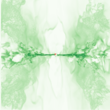
Figure 1: Geometry of the radiation-driven fountain model of Wada et al. (2016). A cross-section of the density grid is shown with the X-ray emitting corona indicated by the red cross. The side length of the simulation region is $32\mathrm{pc}$.

Wada (2012) developed a model in which the obscurer is a radiation pressure-driven polar outflow from a black hole accreting within a thick, parsec-scale disk. The outflow falls back akin to a fountain (see Figure 1) and forms a torus-like shape producing suitably high covering factors (Wada, 2015). In Wada et al. (2016), supernova feedback is also included. The evolution of this system was computed with three-dimensional radiation hydrodynamic simulations on a $256^{3}$ cell grid spanning a domain of $(32\mathrm{pc})^{3}$. As a representation of this model, we use the Wada et al. (2016) geometry from their final simulation time step. Figure 1 shows the geometry for a black hole mass of $M_{{\rm BH}}=2\times 10^{6}M_{\odot}$ and 20% Eddington rate, suitable for comparison to Circinus (see Wada et al., 2016, 2018a; Izumi et al., 2018; Wada et al., 2018b, for comparison with infrared SEDs, atomic/molecular gas, and ionized gas observations, respectively). The model has a Compton-thick LOS column density only under edge-on viewing angles (consistent with the infrared analysis of Circinus by Wada et al., 2016).

The X-ray spectrum under this geometry is computed by placing the X-ray corona at the centre of the simulations density grid (see Figure 1). We use XARS to irradiate the geometry with $5\times 10^{9}$ photons, and capture the energy and direction of X-ray photons escaping to infinity. The direction is used to divide photons by viewing angle in two steps. First, the LOS column density (${N_{\rm{H}}}$) from the corona to infinity in that direction is computed, which defines the first binning axis. Secondly, we further sub-divide by azimuthal angle (face-on to edge-on). This scheme (also in Buchner et al., 2019) has the benefit of separating out the most important observable (LOS ${N_{\rm{H}}}$), and allowing varying the LOS ${N_{\rm{H}}}$ and viewing angle independently.

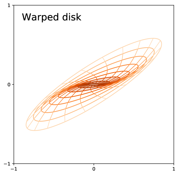
Figure 2: Warped disk geometry, viewed edge-on. Near the centre the disk is only mildly warped (shaded inner-most two annuli, $r_{\text{warp}}\sim 0.25$), and viewing angles are defined relative to there. The outer disk annuli (up to radius $r_{\text{warp}}=1$) are warped more strongly and form a wall, suitable for Compton reflection. For our simulation, we set up a grid with $256^{3}$ cells and assign cells intersecting with this shape a Compton-thick column density.

3.2 Warped disk

Warped, tilted and twisted disks have been proposed as the source of (Compton-thick) obscuration (e.g., Lawrence & Elvis, 2010). Non-planar accretion can cause precessing concentric rings of accretion disks (Petterson, 1977a). Additionally, the disk emits normal to the local surface, but the received radiation pressure from the centre is misaligned and causes torque, and thus twisted disks (Petterson, 1977b). The shape distortion is limited by viscosity, as gas moves radially inward.

Water maser disks are one type of such warped disks known to exist in several AGN. Strongly emitting disk clumps trace out edge-on warped disk structures, e.g. in Circinus (Greenhill et al., 2003). Recently, Jud et al. (2017) developed an infrared model for the warped disk. They demonstrate good fits to infrared photometry and can naturally explain the offset between point source and disk component seen in the highest resolution infrared VLTI observations (Tristram et al., 2014). Water maser disk systems are always found to be heavily obscured (Greenhill et al., 2008; Masini et al., 2016), indicating that the Compton-thick obscurer either is the warped maser disk itself or at least shares the same plane of orientation.

We now simulate such a warped disk obscurer. Pringle (1996) describes the geometry of a warped disk as

$$x = r\cdot(\sin\phi\cos\gamma\cos\beta+\cos\phi\sin\gamma)$$

$$y = r\cdot(\sin\phi\sin\gamma\cos\beta-\cos\phi\cos\gamma)$$

$$z = r\cdot(-\sin\phi\sin\beta)$$

with $\gamma(r)=\sqrt{r}$ and $\beta(r)=\sin(\gamma(r))/\gamma(r)$, following Maloney et al. (1996). The parametrisation essentially describes a disk ring at radius $r$ across angles $\phi\in[0,2\pi]$. We set up a computation grid of $256^{3}$ cells and assign a column density of ${N_{\rm{H}}}=10^{25}\mathrm{cm}^{-2}$ to all grid cells intersecting the warped disk, as well as the cells just below to produce a thickness of at least two grid cells everywhere.

We set up various warp strengths. We let the radii $r$ range from zero (the centre) up to $r_{\text{warp}}=1$, $1/2$, $1/4$ or $1/16$. The case of a strong warp ($r_{\text{warp}}=1$) is illustrated in Figure 2 and features a prominent wall. For $1/4$ and $1/16$, only the flat thin (unwarped) inner disk remains, illustrated as the inner annuli of Figure 2.

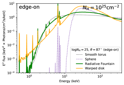
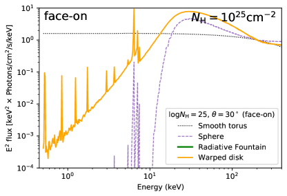
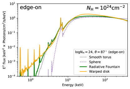
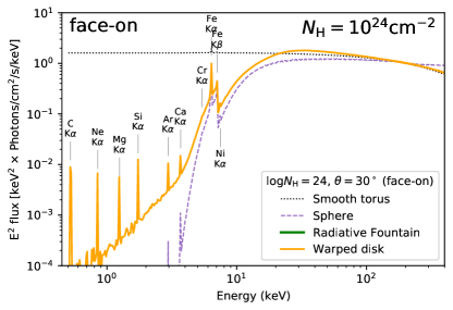
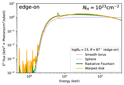
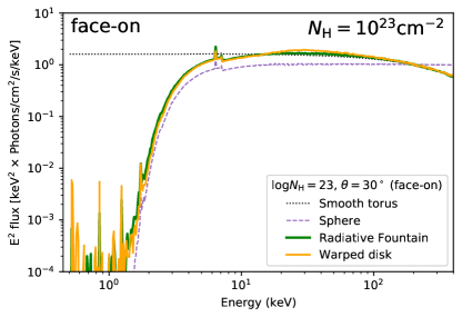
Figure 3: Model spectra of the radiative fountain model (green) and warped disk model (orange). The rows show different line-of-sight column densities. The left/right column shows a nearly edge-on/face-on view of the obscurer. For comparison, a spherical obscurer (Brightman & Nandra, 2011) and smooth torus (Murphy & Yaqoob, 2009) are included as purple dashed and black dotted curves, respectively. In low column densities (bottom row) the predictions are similar. In the right column, the radiative fountain predictions are absent because near-Compton-thick column densities only occur in the equatorial plane. Similarly, the torus is unobscured from this viewing angle and shows the input powerlaw. The models differ most in the $2\textrm{--}20\mathrm{keV}$ range under high obscuring column densities (top left panel). The warped disk produces the strongest emission near $20\mathrm{keV}$ among the models. Models are normalised at $200\,\mathrm{keV}$. The center right panel annotates the included fluorescent lines.

4 Results

4.1 Continuum shapes

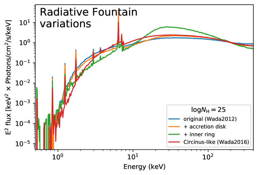
Figure 4: Variations of the radiative fountain model spectra. The Wada (2012) and Wada et al. (2016) models (blue and red, respectively) differ in black hole mass and supernova feedback. The orange curve includes reflection from an accretion disk. The green curve includes a Compton-thick ring around the central X-ray source, which leads to stronger emission in the $10\textrm{--}50\,\mathrm{keV}$ energy range than the original model (blue curve). Models are normalised at $200\,\mathrm{keV}$.

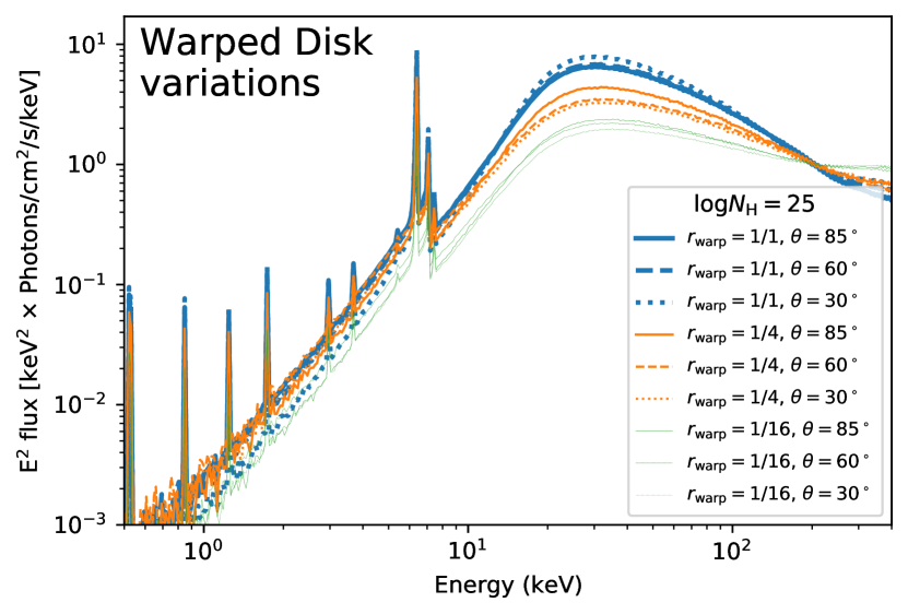
Figure 5: Variations of the warped disk model. Variations of the inclination angle relative to the innermost annuli are represented by solid, dashed and dotted lines. Variations of the extent of the warp (see Figure 2) are represented by line strengths. The thickest lines (strong warps) exhibit the strongest emission in the $20\textrm{--}30\,\mathrm{keV}$ range. Models are normalised at $200\,\mathrm{keV}$.

Examples of obscured spectra are presented in Figure 3. The input photon spectrum is a cut-off powerlaw $E^{-\Gamma}\times\exp(-E/E_{\mathrm{cut}})$ with photon index $\Gamma=2$ and exponential cut-off $E_{\mathrm{cut}}=400\mathrm{keV}$. The panels of Figure 3 plot the emerging $E^{2}\times$photon spectrum, split by inclination and LOS column density. For orientation, we include two models based on simple geometries in Figure 3. The sphere model of Brightman & Nandra (2011) embeds the X-ray point source in a constant-density sphere. This model completely suppresses photons below $10\,\mathrm{keV}$ in Compton-thick sight-lines, except for Fe K fluorescence. The smooth torus model of Murphy & Yaqoob (2009) surrounds the X-ray point source with a constant-density torus, with an opening angle of 60 . Its soft emission is dominated by Compton reflection off the torus. In moderately obscured sight-lines (bottom panels of Figure 3), all models make similar predictions. The sphere model differs slightly from the others, as it does not include an exponential cut-off.

The models differ in the strength of the Compton hump near $10\textrm{--}50\,\mathrm{keV}$. The warped disk model shows the strongest emission, while the radiative fountain model has a weak Compton hump. This is likely related to the high covering factor of high-density material in the warped disk that is seen without further obscuration by the observer. The two models bracket the sphere model in terms of the Compton hump strength. Additionally, the hump shapes are different in their turn-over.

The models differ most strongly in the $2\textrm{--}20\,\mathrm{keV}$ energy range under Compton-thick LOS (e.g., top left panel). Here the transmitted powerlaw continuum is suppressed, revealing the Compton reflected components and fluorescent lines. In both of our two models, soft photons escape under all viewing angles through Compton scattering.

The spectral slopes in the $2\textrm{--}20\,\mathrm{keV}$ energy range are diverse. The spherical obscurer shows the steepest slope among the models. The smooth torus and radiative fountain models show a smooth exponential turn-over, at lower energies than the sphere geometry. In contrast, the warped disk model presents a powerlaw-like continuum in the $2\textrm{--}20\,\mathrm{keV}$ energy range with photon index $\Gamma\approx 0.5$. The warped disk produces the strongest emission near $20\,\mathrm{keV}$ among the models. Its Compton hump is widest in the radiative fountain model.

We explore these differences further in Figure 4 and 5. Figure 4 shows the spectra from the models of Wada (2012) and Wada et al. (2016), which differ primarily in that the latter uses a ten times smaller black hole mass and the presence of supernova feedback, both chosen to match the Circinus Galaxy. The X-ray spectral predictions are however of similar shape, characterised by a smoothly bending reflection spectrum in the $2\textrm{--}20\,\mathrm{keV}$ energy range. The resulting spectra are very similar across viewing angles, if the LOS column density are kept constant. However, Compton-thick sight-lines, as shown in Figure 4, only exist in equatorial views.

4.2 Model variations

Reflection close to the X-ray corona can alter the spectral shape. The accretion disk is a known reflector, and can be modelled by a semi-infinite slab. We replace the input powerlaw source with a powerlaw source and its disk-reflected, angle-averaged spectrum. The disk model spectrum was computed with XARS and presented in the appendix of Buchner et al. (2019), and is consistent with the pexmon disk model (Nandra et al., 2007). The effect of the accretion disk model can be seen by comparing the orange curve in Figure 4 with the blue curve. The model with accretion disk (orange) shows a higher Compton hump than the model without (blue). However, the difference is less than a factor of 2. This may be because the disk adds reflection, but does not hinder the powerlaw emission from the X-ray source over half of the sky.

Higher covering factor obscuring structure at small scales have more drastic changes. We experiment how the fountain model would need to be minimally changed to behave like the warped disk model. At the same time, the ultra-violet radiation pressure of the model should remain unaffected. A completely ionised structure between accretion disk and $<0.1\mathrm{pc}$ scales may be a viable solution. This could be similar to the dense, inner shielding gas of wind simulations by Gallagher et al. (2015), and could also be interpreted as a sub-parsec scale warped disk, or the broad line region. For simplicity, we achieve a toroid with a opening angle of approximately 60 , by setting the eight spaxels closest to the X-ray emitter in the equatorial plane to Compton-thick column densities. The emerging spectrum is shown in green in Figure 4. The spectral shape is dramatically different, showing a much stronger Compton hump. It is very similar to the warped disk model (see top left panel of Figure 3).

Variations of the warped disk models are shown in Figure 5. The most important parameter is the extent of the warp (increasing with line thickness). For stronger warps (see visualisation in Figure 2), the increased area available for Compton reflection strengthens the Compton hump emission near $20\,\mathrm{keV}$. The viewing angle (defined relative to the innermost annuli) has a minor effect, because of the twisting shape of this geometry.

We publish the spectra as Xspec table models at https://github.com/JohannesBuchner/xars.

4.3 Plausability of models

The model diversity shown in the previous section indicates that in the Compton-thick regime, hard X-ray spectra can differentiate model geometries. As outlined in 2.2, we explore the plausibility of our models by projecting them through the NuSTAR response and comparing against a few, high-quality observations. Typical AGN source parameters (a powerlaw continuum with photon index $\Gamma=2$) are assumed, and the line-of-sight obscuration is varied. As contaminating components all decline steeply with energy, therefore we normalise each model with the data at the high energy end and accept models that do not overpredict the data.

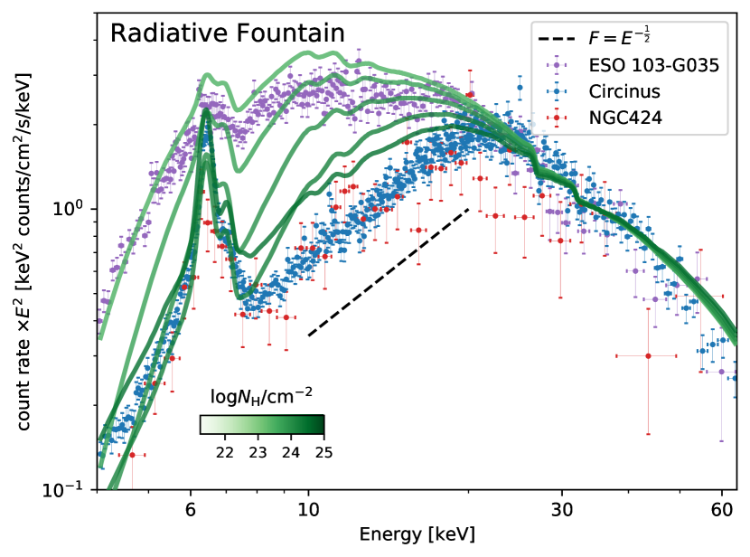
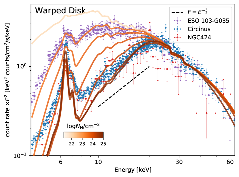
Figure 6: Comparison of radiative fountain model (top panel) and warped disk model (bottom) to three observed spectra of AGN (error bars). Each panel shows one fixed model geometry. Model instances with photon index $\Gamma=2$ and LOS column densities of $\log{N_{\rm{H}}}=20,23.5,23.75,24,24.25,24.5,26$ (top to bottom curves) are folded through the three instrument responses (near-overlapping groups of curves). Data and models are normalised at $35\,\mathrm{keV}$. Top panel: The radiative fountain models show an excess near $10\mathrm{\,keV}$ compared to the data. Bottom panel: The warped disk model follows the ESO 103-G035 data closely, and also reproduces the Circinus data. The models underproduce the data at $4\textrm{--}8\,\mathrm{keV}$.

Figure 6 shows three NuSTAR spectra of nearby AGN. The high-quality data reveals the reflector in great detail. The top panel of Figure 6 compares spectra from the radiative fountain model (green) to the data. An input power law with photon index of $\Gamma=2$ is seen through varying layers of column density (green curves). The data of ESO 103-G035 mostly match some of the top model curves, but the $8\textrm{--}10\mathrm{keV}$ data is underpredicted. This could be accommodated by additional soft energy emission components. The situation is more discrepant when considering the Circinus Galaxy. While the data show a powerlaw-like increase from 8 to 20 keV, the models present a wide hump from 8 to $20\,\mathrm{keV}$. The models overpredict the data at $10\textrm{--}25\,\mathrm{keV}$ even at the highest column densities (lowest curve). A better result may be possible, if an additional reflector was included (see Figure 4). The data of NGC 424 mimic those of the Circinus Galaxy, but have larger uncertainties.

The bottom panel of Figure 6 compares spectra from the warped disk model (orange) to the data. Here, the data of ESO 103-G035 are directly reproduced by the model, in terms of the $3\textrm{--}6\mathrm{keV}$ slope, the $8\textrm{--}20\mathrm{keV}$ shape and the Compton hump strength. The same is true for NGC 424. For the Circinus Galaxy, the data can be matched well from $10\,\mathrm{keV}$ upwards. At energies below $10\,\mathrm{keV}$, an additional contribution appears to be needed. This is expected. In Buchner et al., 2019 and many other works, an additive powerlaw component has been employed for this purpose. The photon index $\Gamma$ has not been tuned, which could lead to even better agreement. The projection of the warped disk model onto the data is encouraging. To test this more thoroughly, the multiple spectral components and their model parameters have to be fitted jointly.

4.4 Test case: Spectral fit to Circinus

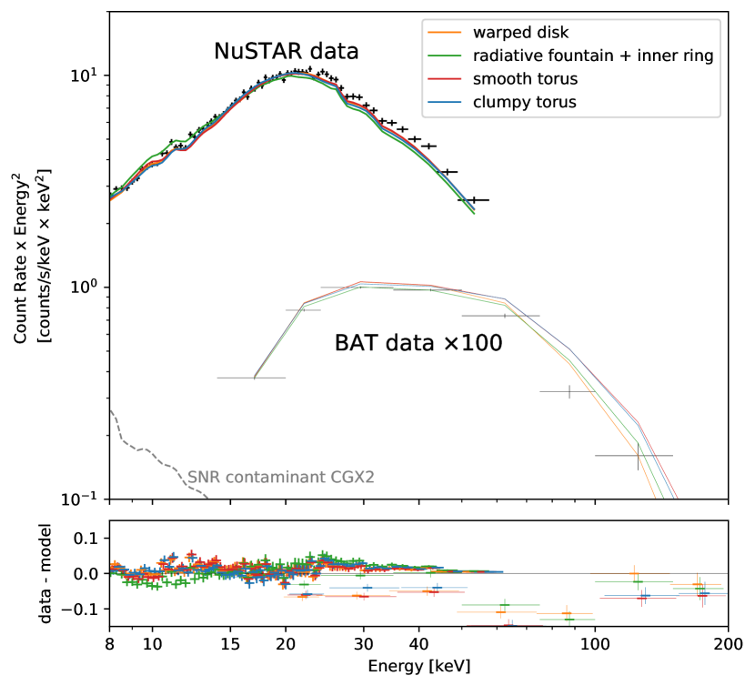
Figure 7: Circinus hard X-ray spectrum with fitted models. The NuSTAR $8-75\mathrm{\,keV}$ (here heavily rebinned just for visualisation) and BAT $15-150\mathrm{\,keV}$spectra were fitted with four models. The warped disk model yields the lowest $\chi\text{\texttwosuperior}$.

Table 1: Best-fit models parameters for the Circinus Galaxy.

Model Geometry	${N_{\rm{H}}}$	$\Gamma$	$f_{\mathrm{scat}}$	$\theta_{\mathrm{incl}}$	$\chi^{2}$/dof
	$10^{24}\mathrm{cm}^{-2}$		$\%$
(various, in Arévalo et al., 2014)	$3\textrm{--}20$	$1.6\textrm{--}2.5$		$\sim 75$	-
Smooth torus	$6.4\pm 0.4$	$\geq 2.6$	$\leq 5\times{10}^{-3}$	$81.8\pm 0.5$	1502/1463
Clumpy torus	$\geq 9.93$	$2.43\pm 0.03$	$30\pm 6\times{10}^{-2}$	$\geq 85$	1523/1462
Warped disk	$12.61\pm 3.30$	$2.00\pm 0.01$	$2.9\pm 1.3\times{10}^{-3}$	$51\pm 21$	1432/1462
Radiative fountain + inner ring	$16\pm 1$	$1.97\pm 0.007$	$\leq 3\times{10}^{-4}$	$82\pm 8$	1451/1463

Finally, a full spectral fit is performed to the data from the Circinus Galaxy. This object is most suitable, because the hydrodynamic simulations of the radiative fountain model have been tailored to its parameters (accretion rate and black hole mass). Appendix B makes comparisons to the other two galaxies considered in this work. The observed spectrum from NuSTAR and Swift/BAT, presented in Figure 7, also exhibits high photon count statistics. For clear presentation, the NuSTAR spectra were summed and rebinned to 1000 counts per bin, but for fitting we use a spectrum binned to 20 counts per bin.

Four spectral models of the obscurer geometry are considered. From this work, the warped disk model and the radiative fountain model with the inner ring modification are included. The smooth torus geometry of Murphy & Yaqoob (2009) and the clumpy torus of Liu & Li (2014) are also considered. In addition to a powerlaw source processed by an obscurer model, two further components are included. A secondary, unobscured powerlaw is included with the same photon index and a normalisation $f_{\mathrm{scat}}$ of up to $10\%$ of the primary powerlaw normalisation. The CGX2 supernova remnant contamination has been included as a frozen mekal component with values taken from Arévalo et al. (2014). The spectrum was fitted with all parameters controlling the spectral shape (${N_{\rm{H}}}$, $\Gamma$, $f_{\mathrm{scat}}$) free to vary. The normalisation in each data set (FPMA, FPMB, BAT) were left free to vary independently, to account for cross-calibration factors.

We report the most important spectral parameters in Table 1. The fit $\chi^{2}$ statistic is best in the warped disk model ($\chi^{2}/\mathrm{dof}=1432/1462$). The radiative fountain model is a good fit when an inner ring is inserted ($\chi^{2}/\mathrm{dof}=1451/1463$), but not without ($\chi^{2}/\mathrm{dof}=4392/1463$). In both models the photon index is $\Gamma=2$, close to typical values in the population ($\Gamma=1.95\pm 0.15$, Nandra & Pounds 1994; Ricci et al. 2017). The clumpy torus ($\chi^{2}/\mathrm{dof}=1523/1462$) and the smooth torus ($\chi^{2}/\mathrm{dof}=1502/1463$) do not fit the data as well. The NuSTAR data force these models to high, atypical photon indices ($\Gamma>2.4$), which are disfavored by the Swift/BAT data ($\Gamma=2.09\pm 0.02$ in Oh et al., 2018). All models indicate very high column densities (${N_{\rm{H}}}\geq 10^{25}\mathrm{cm}^{-2}$). For reference, we also list the parameters found in the recent detailed analysis of Arévalo et al. (2014), which considered a multitude of models, including the smooth torus model.

5 Discussion & Conclusion

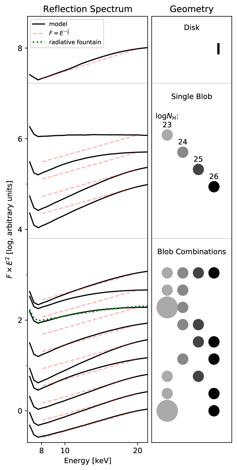
Figure 8: Reflection spectrum (left, black) for different geometries (right). Black curves are normalised at $20\,\mathrm{keV}$, with offsets. The red dashed lines illustrate the observed power law. The top example shows reflection off a semi-infinite disk. The middle four examples show a single blob with column densities $\log{N_{\rm{H}}}=23,\,24,\,25$ and $26$. In low-density blobs, the reflection extends to low energies, while for the densest blobs the spectrum rises rapidly (powerlaw photon index $\approx 0$). The bottom examples show mixtures of the reflection spectra, assuming equal covering factors in all but the last. Mixtures have a wider Compton hump with a smooth bend. The exceptions are the bottom three examples, which lack the $\log{N_{\rm{H}}}=24$ blob. Their powerlaw-like spectrum approximately follows $F\propto E^{-\frac{1}{2}}$ (red dashed line). The dotted green line shows the radiative fountain model.

In this work we have extended the open source XARS Monte Carlo spectra simulation software to irradiate arbitrary density grids. We explore physically motivated geometries, including Wada’s radiative fountain model and warped disks. This allows for the first time investigation of gas geometries predicted by hydro-dynamic simulations.

5.1 Geometry information in X-ray spectra

Different geometries of AGN obscurers predict very different X-ray spectra. In particular, powerful indicators of the obscurer geometry in heavily obscured AGN are illustrated by the top left panel of Figure 3. These include the continuum slope just below the Fe K emission feature ($2-6\,\mathrm{keV}$), the bend of the continuum between the Fe K edge and the Compton hump ($8\textrm{--}20\,\mathrm{keV}$). Below we discuss how different geometries produce different shapes.

Spherical, completely covering obscurers predict virtually no escape of continuum photons below $10\,\mathrm{keV}$. Such geometries have been suggested for merging galaxies, but are difficult to test because of the low-energy contamination by stellar processes in these often star-bursting galaxies (e.g., Arp 220, see Teng et al., 2015).

The reflection processes are more elaborate in other geometries. Warped disks, sight-lines through the disk heavily suppress the continuum, while an elevated far side can provide an unabsorbed reflection spectrum. This behaviour resembles smooth torus geometries (Murphy & Yaqoob, 2009), where the far side also provides substantial reflection.

The warped disk structure requires much less mass than a smooth torus, and is dynamically stable. The extent of the warp is related to the covering factor and influences the strength of the Compton hump emission (see Figure 5).

The radiative fountain model is more complex. A mixture of constant-density spheres can help understand the emerging spectral shape. The reflection off a single, spherical blob in the $8\textrm{--}20\leavevmode\nobreak\ \mathrm{keV}$ band is shown in Figure 8 (middle four cases, from the Appendix of Buchner et al., 2019). High-density blobs show a steeply rising spectrum, while low-density blobs also let low-energy photons escape. Combining low, intermediate and high-density blobs is shown in the bottom of Figure 8. The mixture of these reflection spectra leads to a wide, smooth hump. Such a spectrum emerges from the radiative fountain model (dotted green curve). In that model, photons interact with a wide range of mostly Compton-thin densities as they travel towards infinity. The truncation towards soft energies in Figure 3 can be explained by photo-electric absorption by a Compton-thin gas envelope.

5.2 The obscuring structure of nearby galaxies

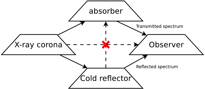
Figure 9: Inferred unobscured line-of-sights in Compton-thick AGN. Arrows indicate unobscured lines of sight between components. Importantly, the reflection is not reprocessed by the absorber, and the corona is not directly observed (red cross). The reflector is illuminated by the corona directly, not the absorbed emission. The warm mirror is not shown, but would have similar relations as the cold reflector. The host and Milky Way galaxy absorbing screens are also not shown.

High-quality high-energy spectra from nearby galaxies enable differentiating obscurer geometries. Indeed, the warped disk model was selected as the best fit to the Circinus Galaxy. However, a more generic conclusion can be drawn. The observed spectrum evinces a power law of $E^{-\frac{1}{2}}$ in the $8\textrm{--}20\,\mathrm{keV}$ energy window (dashed line in Figure 6). A preliminary analysis of more AGN observed with NuSTAR indicates that such spectral shapes occur only in rapidly accreting AGN with Eddington accretion ratios of $\dot{M}/\dot{M}_{Edd}\gtrsim 20\%$. The examples in Figure 8 illustrate that such photon flux shapes are only possible with a bimodal distribution of blob densities, including heavily Compton-thick blobs and thinner blobs ${N_{\rm{H}}}\lesssim 10^{23}\mathrm{cm}^{-2}$. For the radiative fountain model, this suggests that if the thick disk was denser, the model may follow the data better. Another way to achieve this result, illustrated by the orange curve in Figure 4, is to insert an inner high-covering obscuring structure. This effectively prevents X-ray reflection from the thick disk and alters the spectrum substantially. A very similar conclusion was reached by Buchner et al. (2019), who inserted a inner ring into a clumpy obscurer model.

Figure 9 illustrates the generic recipe to produce the observed shapes. Firstly, the observed spectrum is reflection-dominated, therefore the sightline between observer and the X-ray corona features the Compton-thick obscuration. Secondly, Compton-thick reflecting surfaces with high covering factors are required to have unobscured sight-lines both to the observer and the X-ray corona. The accretion disk is unsuitable for this (see Figure 4). This is because in non-relativistic, flat accretion disks the disk reflection and powerlaw both pass through the absorber (dashed, crossed out arrow in Figure 9). In contrast, warped disks are one way to provide Compton-thick reflection surfaces that see the corona and the observer unobscured (bottom arrows in Figure 9). The analysed spectra (Figure 6 and 8) also place upper limits on reflection from Compton-thin column densities.

Nevertheless, there are substantial caveats to our conclusions. The nuclear reflection on parsec and sub-parsec scales needs to be separated by a combination of NuSTAR and Chandra observations. In the future, higher angular resolution missions such as Lynx (The Lynx Team, 2018) will provide additional separation. However, also a wider variety of simulations with higher spatial resolution is desired. Additionally, ionisation cone imaging spectroscopy (in optical and X-rays) could be used to constrain the coherence and opening angle of the inner structure (see e.g., Zhao et al., 2020).

5.3 Implications and outlook

The spectral model diversity in the Compton-thick regime has important implications. Firstly, the model choice affects the selection of Compton-thick AGN, and the computation of their space density. Many recent surveys (e.g., Ueda et al., 2014; Buchner et al., 2015; Aird et al., 2016) rely on the spectral model of Brightman et al. (2015). A fixed spectral model is used to compute the sensitivity to detecting Compton-thick AGN as a function of redshift and luminosity. Ricci et al. (2015) explicitly demonstrated that the derived Compton-thick fraction varies with the assumed geometry. Thus, knowing the geometry is crucially important. Secondly, hardness ratios and luminosity absorption corrections in the Compton-thick regime are strongly dependent on the model geometry, in particular when analysing band counts (e.g., $0.5\textrm{--}2\,\mathrm{keV}$ and $2\textrm{--}10\,\mathrm{keV}$) with a fixed spectral model. Recovering the intrinsic accretion luminosity is more reliable when using multi-component spectral fits for each object instead (e.g., Buchner et al., 2014).

Investigation of spectra of nearby AGN suggests evidence of extreme column densities of ${N_{\rm{H}}}>10^{25}\mathrm{cm}^{-2}$. These are needed either along the LOS (see Table 1) or are present outside the LOS in the models not excluded by the data (see Figure 6 and Buchner et al., 2019). Such high column densities are outside the range of most previous models. This is in part because the many photon interactions in such dense media are computationally costly to evaluate. XARS provides an efficient implementation for such situations to address this, and can illuminate arbitrarily complex geometries. In part, such high column densities (${N_{\rm{H}}}>10^{25}\mathrm{cm}^{-2}$) have not been considered because they seem to be rare and unlikely a priori. However, current X-ray surveys of AGN may miss these, as they become strongly absorbed even in the highest energy surveys (e.g., Swift/BAT), and additional multi-wavelength selection methods may need to be developed to complement them. However, strong conclusions require the analysis of a representative and complete sample. Systematic NuSTAR follow-up of the Swift/BAT survey is currently the most promising avenue Baloković (2017), with careful multi-component and spatially resolved analyses of NuSTAR, XMM-Newton and Chandra data to separate non-AGN contributions and extended reflection (as in, e.g., Arévalo et al., 2014; Bauer et al., 2015). Because of the complex parameter degeneracies (between geometry parameters, the LOS ${N_{\rm{H}}}$, and source luminosity, $\Gamma$ and $E_{\mathrm{cut}}$), reliable fits require global parameter exploration algorithms such as nested sampling (as, e.g., in Buchner et al., 2014).

Different models retrieve different photon indices in the Compton-thick regime. Even when only $>8\,\mathrm{keV}$ data are considered, the effect size, $\Delta\Gamma\approx 0.4$, is substantially larger than the uncertainties (see Table 1). Under the assumption that the accretion proceeds the same at the same Eddington ratio, the photon index distribution should be the same in Compton-thin AGN and Compton-thick AGN. This can provide an additional test of the geometry, even when multiple geometries provide equally good fits per-source. For example, Ueda et al. (2014) find different photon indices for unobscured and moderately obscured AGN, which are not seen in the local Universe when high-energy data are available (Ricci et al., 2017), and may point to an incomplete modelling assumption. A similar test can be done also with the energy cut-off parameter, which can yield low values ($E_{\mathrm{cut}}<50\,\mathrm{keV}$) in incomplete models.

6 Acknowledgements

We thank the anonymous referees for constructive suggestions which improved the manuscript.

We acknowledge support from the CONICYT-Chile grants Basal-CATA PFB-06/2007 (JB, FEB), ANID grants CATA-Basal AFB-170002 (JB, FEB), FONDECYT Regular 1141218, 1190818 and 1200495 (all FEB), FONDECYT Postdoctorados 3160439 (JB), “EMBIGGEN” Anillo ACT1101 (FEB), and the Ministry of Economy, Development, and Tourism’s Millennium Science Initiative through grant IC120009, awarded to The Millennium Institute of Astrophysics, MAS (JB, FEB). This research was supported by the DFG cluster of excellence “Origin and Structure of the Universe”. MiB acknowledges support from NASA Headquarters under the NASA Earth and Space Science Fellowship Program, the YCAA Prize Postdoctoral Fellowship, grant NNX14AQ07H, and support from the Black Hole Initiative at Harvard University, which is funded in part by the Gordon and Betty Moore Foundation (grant GBMF8273) and in part by the John Templeton Foundation. KW was supported by JSPS KAKENHI Grant Number 16H03959.

This research has made use of the NASA/IPAC Extragalactic Database (NED), which is operated by the Jet Propulsion Laboratory, California Institute of Technology, under contract with the National Aeronautics and Space Administration. This research has made use of SIMBAD (Wenger et al., 2000) and its excellent query API, operated by the Strasbourg astronomical Data Center (CDS).

Appendix A 3D Discrete Digital Analyser

Algorithm 1 A simplified 2D version of our grid traversal algorithm.

⬇

function DDA(

// starting position

double x0, double y0,

// direction

double dx, double dy,

// column density

double NH

) {

// initialisation at current cell

double dt_dx = 1. / dx;

double dt_dy = 1. / dy;

int x, y = x0, y0;

int x_inc, y_inc;

double t_next_x, t_next_y;

int sign_x = 1, sign_y = 1;

if (dx > 0) {

x_inc = 1;

t_next_x = (floor(x0) + 1 - x0) / dx;

} else {

x_inc = -1;

t_next_x = (x0 - floor(x0)) / dx;

sign_x = -1;

}

if (dy > 0) {

y_inc = 1;

t_next_y = (floor(y0) + 1 - y0) / dy;

} else {

y_inc = -1;

t_next_y = (y0 - floor(y0)) / dy;

sign_y = -1;

}

loop {

double last_t = t; int last_x = x, last_y = y;

if (t_next_y*sign_y <= t_next_x*sign_x) {

// go in y

y += y_inc;

t = t_next_y;

t_next_y += dt_dy;

} else {

// go in x

x += x_inc;

t = t_next_x;

t_next_x += dt_dx;

}

// density of this grid cell:

double rho = rhoarr[last_x, last_y];

if ((fabs(t) - last_t) * rho > NH) {

// terminate within this cell.

// return distance travelled

return last_t + NH / rho;

}

// subtract full cell

NH -= (fabs(t) - last_t) * rho;

} // end of loop

} // end of function

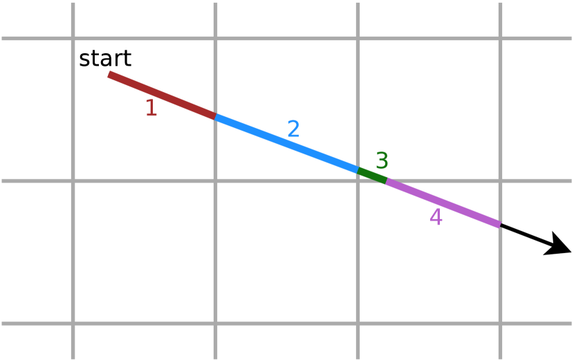
Figure 10: Illustration of photon propagation in a grid. The Discrete Digital Analyser algorithm finds the sequence of points where the line crosses grid boundaries. This allows segmentation of the line by grid cell, illustrated by the numbers and colours.

We briefly describe how density grids were illuminated and processed into X-ray spectra. In XARS (see Buchner et al. 2019), the user needs to specify two functions, one describing the geometry, and the second specifying how escaping photons are gridded (e.g. in viewing angle). For the latter we chose gridding in viewing angle and LOS column density to the corona (see Buchner et al. 2019), as these are the primary aspects affecting the output spectrum. The custom geometry function receives a photon position, direction and ${N_{\rm{H}}}$ distance (in optical depth units) to travel until the photons stops (for interaction with the medium).

In the case of our density grids, the density within a grid cell is assumed to be constant. The problem then transforms to measuring the distances traversed in each grid cell and multiplying with the grid density to obtain the grid cells ${N_{\rm{H}}}$. We illustrate the segmentation of the path in Figure 10. This is subtracted from the target ${N_{\rm{H}}}$ distance until it reaches zero. Measuring the distances traversed in each grid cell is solved with a 3D Discrete Digital Analyser, an algorithm developed for drawing lines through pixels in computer graphics (Fujimoto et al. 1986). We present a two-dimensional simplified version in Figure 1; the extension to three dimensions is straight-forward. The algorithm computes the step size between grid lines given the current direction, and then steps through the grid cells in the right order (either in x or y). The outlined algorithm returns the coordinate space distance traversed until the photon has travelled through a column density of ${N_{\rm{H}}}$.

Appendix B Spectral fits of NGC 3393 and NGC 424

For completeness, we also present spectral fits for the two other galaxies, NGC 3393 and NGC 424. The setup is virtually identical to that described in section 4.4. The only difference in the modelling is that no SNR contaminant is included.

Figure 11 presents the spectral fit of five models. All models give good fit qualities ($\chi^{2}/\mathrm{dof}<80/77$). However, the best fit photon indices of the clumpy model and the radiative fountain model are low ($1.69\text{$\pm$}0.11$ and $1.53\pm 0.16$, respectively). For the other models, including the radiative fountain model with inner ring, the best fit photon index has values more typical of the population (the $1.8-2.0$ interval overlaps the $1\sigma$ confidence intervals). All model fits produce best-fit column densities in the Compton-thick regime.

Figure 12 presents the equivalent spectral fit for NGC 424. All models give good fit qualities ($\chi^{2}/\mathrm{dof}\lesssim 115/128$). However, the best fit photon indices of the clumpy torus model and the smooth torus model are high ($2.46\text{$\pm$}0.27$ and $2.45\pm 0.26$, respectively). For the other models, the best fit photon index hav values typical of the population ($2.0$ is within the $1\sigma$ confidence intervals). All model fits produce best-fit column densities in the Compton-thick regime.

The spectral fits confirm the point of Figure 6: The spectra can be explained by an AGN with a typical photon index $\Gamma=2$ under the warped disk model, but not under the radiative fountain model, unless a inner ring is added.

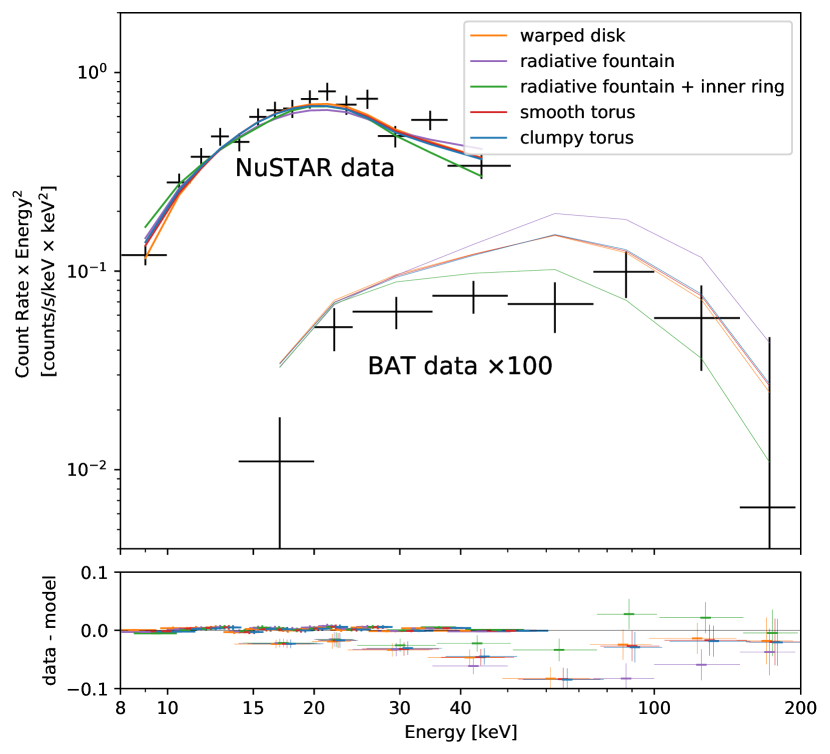
Figure 11: Same as Figure 7, but for NGC 3393.

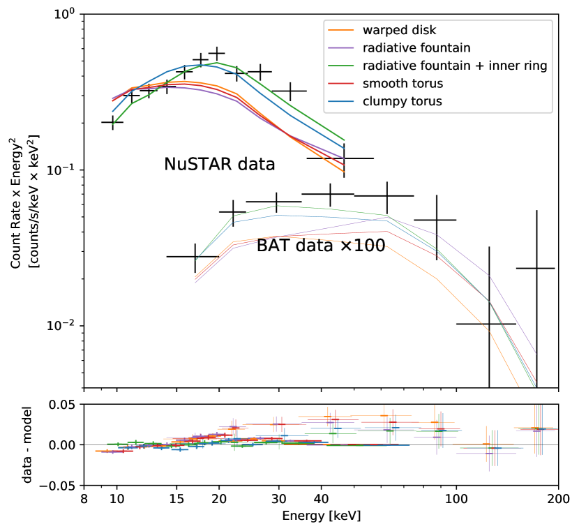
Figure 12: Same as Figure 7, but for NGC 424.

References

- Aird et al. (2016) Aird, J., Coil, A. L., & Georgakakis, A. 2016, ArXiv e-prints
- Anders & Grevesse (1989) Anders, E. & Grevesse, N. 1989, Geochim. Cosmochim. Acta., 53, 197
- Antonucci (1993) Antonucci, R. 1993, ARA&A, 31, 473
- Arévalo et al. (2014) Arévalo, P., Bauer, F. E., Puccetti, S., et al. 2014, ApJ, 791, 81
- Baloković (2017) Baloković, M. 2017, PhD thesis, California Institute of Technology
- Baloković et al. (2018) Baloković, M., Brightman, M., Harrison, F. A., et al. 2018, ArXiv e-prints
- Baloković et al. (2014) Baloković, M., Comastri, A., Harrison, F. A., et al. 2014, ApJ, 794, 111
- Bauer et al. (2015) Bauer, F. E., Arévalo, P., Walton, D. J., et al. 2015, ApJ, 812, 116
- Bianchi et al. (2006) Bianchi, S., Guainazzi, M., & Chiaberge, M. 2006, A&A, 448, 499
- Brightman et al. (2015) Brightman, M., Baloković, M., Stern, D., et al. 2015, ApJ, 805, 41
- Brightman & Nandra (2011) Brightman, M. & Nandra, K. 2011, MNRAS, 413, 1206
- Brightman et al. (2014) Brightman, M., Nandra, K., Salvato, M., et al. 2014, MNRAS, 443, 1999
- Buchner & Bauer (2017) Buchner, J. & Bauer, F. E. 2017, MNRAS, 465, 4348
- Buchner et al. (2019) Buchner, J., Brightman, M., Nandra, K., Nikutta, R., & Bauer, F. E. 2019, A&A, 629, A16
- Buchner et al. (2015) Buchner, J., Georgakakis, A., Nandra, K., et al. 2015, ApJ, 802, 89
- Buchner et al. (2014) Buchner, J., Georgakakis, A., Nandra, K., et al. 2014, A&A, 564, A125
- Buchner et al. (2017) Buchner, J., Schulze, S., & Bauer, F. E. 2017, MNRAS, 464, 4545
- Chan & Krolik (2016) Chan, C.-H. & Krolik, J. H. 2016, ApJ, 825, 67
- Dorodnitsyn & Kallman (2017) Dorodnitsyn, A. & Kallman, T. 2017, ApJ, 842, 43
- Fabbiano et al. (2018) Fabbiano, G., Paggi, A., Karovska, M., et al. 2018, ApJ, 855, 131
- Fujimoto et al. (1986) Fujimoto, A., Tanaka, T., & Iwata, K. 1986, IEEE Computer Graphics and Applications, 6, 16
- Furui et al. (2016) Furui, S., Fukazawa, Y., Odaka, H., et al. 2016, ApJ, 818, 164
- Gallagher et al. (2015) Gallagher, S. C., Everett, J. E., Abado, M. M., & Keating, S. K. 2015, MNRAS, 451, 2991
- Gandhi et al. (2014) Gandhi, P., Lansbury, G. B., Alexander, D. M., et al. 2014, ApJ, 792, 117
- Gaspari et al. (2015) Gaspari, M., Brighenti, F., & Temi, P. 2015, A&A, 579, A62
- Greenhill et al. (2003) Greenhill, L. J., Booth, R. S., Ellingsen, S. P., et al. 2003, ApJ, 590, 162
- Greenhill et al. (2008) Greenhill, L. J., Tilak, A., & Madejski, G. 2008, ApJ, 686, L13
- Hopkins et al. (2012) Hopkins, P. F., Hayward, C. C., Narayanan, D., & Hernquist, L. 2012, MNRAS, 420, 320
- Ikeda et al. (2009) Ikeda, S., Awaki, H., & Terashima, Y. 2009, ApJ, 692, 608
- Izumi et al. (2018) Izumi, T., Wada, K., Fukushige, R., Hamamura, S., & Kohno, K. 2018, ApJ, 867, 48
- Jud et al. (2017) Jud, H., Schartmann, M., Mould, J., Burtscher, L., & Tristram, K. R. W. 2017, MNRAS, 465, 248
- Lawrence & Elvis (2010) Lawrence, A. & Elvis, M. 2010, ApJ, 714, 561
- Liu & Li (2014) Liu, Y. & Li, X. 2014, ApJ, 787, 52
- Magdziarz & Zdziarski (1995) Magdziarz, P. & Zdziarski, A. A. 1995, MNRAS, 273, 837
- Maloney et al. (1996) Maloney, P. R., Begelman, M. C., & Pringle, J. E. 1996, ApJ, 472, 582
- Marinucci et al. (2013) Marinucci, A., Miniutti, G., Bianchi, S., Matt, G., & Risaliti, G. 2013, MNRAS, 436, 2500
- Markowitz et al. (2014) Markowitz, A. G., Krumpe, M., & Nikutta, R. 2014, MNRAS, 439, 1403
- Masini et al. (2016) Masini, A., Comastri, A., Baloković, M., et al. 2016, A&A, 589, A59
- Matt et al. (2000) Matt, G., Fabian, A. C., Guainazzi, M., et al. 2000, MNRAS, 318, 173
- Matt et al. (1999) Matt, G., Pompilio, F., & La Franca, F. 1999, New A, 4, 191
- Mościbrodzka & Proga (2013) Mościbrodzka, M. & Proga, D. 2013, ApJ, 767, 156
- Murphy & Yaqoob (2009) Murphy, K. D. & Yaqoob, T. 2009, MNRAS, 397, 1549
- Nandra et al. (2007) Nandra, K., O’Neill, P. M., George, I. M., & Reeves, J. N. 2007, MNRAS, 382, 194
- Nandra & Pounds (1994) Nandra, K. & Pounds, K. A. 1994, MNRAS, 268, 405
- Nenkova et al. (2008) Nenkova, M., Sirocky, M. M., Ivezić, Ž., & Elitzur, M. 2008, ApJ, 685, 147
- Netzer (2015) Netzer, H. 2015, ARA&A, 53, 365
- Oh et al. (2018) Oh, K., Koss, M., Markwardt, C. B., et al. 2018, ApJS, 235, 4
- Petterson (1977a) Petterson, J. A. 1977a, ApJ, 214, 550
- Petterson (1977b) Petterson, J. A. 1977b, ApJ, 216, 827
- Pringle (1996) Pringle, J. E. 1996, MNRAS, 281, 357
- Ramos Almeida & Ricci (2017) Ramos Almeida, C. & Ricci, C. 2017, Nature Astronomy, 1, 679
- Ricci et al. (2017) Ricci, C., Trakhtenbrot, B., Koss, M. J., et al. 2017, ApJS, 233, 17
- Ricci et al. (2015) Ricci, C., Ueda, Y., Koss, M. J., et al. 2015, ApJ, 815, L13
- Risaliti et al. (2002) Risaliti, G., Elvis, M., & Nicastro, F. 2002, ApJ, 571, 234
- Rivers et al. (2013) Rivers, E., Markowitz, A., & Rothschild, R. 2013, ApJ, 772, 114
- Schartmann et al. (2018) Schartmann, M., Mould, J., Wada, K., et al. 2018, MNRAS, 473, 953
- Tanimoto et al. (2019) Tanimoto, A., Ueda, Y., Odaka, H., et al. 2019, ApJ, 877, 95
- Teng et al. (2015) Teng, S. H., Rigby, J. R., Stern, D., et al. 2015, ApJ, 814, 56
- The Lynx Team (2018) The Lynx Team. 2018, arXiv e-prints, arXiv:1809.09642
- Tristram et al. (2014) Tristram, K. R. W., Burtscher, L., Jaffe, W., et al. 2014, A&A, 563, A82
- Turner et al. (1997) Turner, T. J., George, I. M., Nandra, K., & Mushotzky, R. F. 1997, ApJ, 488, 164
- Ueda et al. (2014) Ueda, Y., Akiyama, M., Hasinger, G., Miyaji, T., & Watson, M. G. 2014, ApJ, 786, 104
- Ueda et al. (2003) Ueda, Y., Akiyama, M., Ohta, K., & Miyaji, T. 2003, ApJ, 598, 886
- Verner et al. (1996) Verner, D. A., Ferland, G. J., Korista, K. T., & Yakovlev, D. G. 1996, ApJ, 465, 487
- Wada (2012) Wada, K. 2012, ApJ, 758, 66
- Wada (2015) Wada, K. 2015, ApJ, 812, 82
- Wada et al. (2018a) Wada, K., Fukushige, R., Izumi, T., & Tomisaka, K. 2018a, ApJ, 852, 88
- Wada et al. (2016) Wada, K., Schartmann, M., & Meijerink, R. 2016, ApJ, 828, L19
- Wada et al. (2018b) Wada, K., Yonekura, K., & Nagao, T. 2018b, ApJ, 867, 49
- Wenger et al. (2000) Wenger, M., Ochsenbein, F., Egret, D., et al. 2000, A&AS, 143, 9
- Williamson et al. (2018) Williamson, D., Venanzi, M., & Hönig, S. 2018, arXiv e-prints, arXiv:1812.07448
- Zhao et al. (2020) Zhao, X., Marchesi, S., Ajello, M., balokovic, M., & Fischer, T. 2020, arXiv e-prints, arXiv:2003.12190