Generating Data Augmentation samples for Semantic Segmentation of Salt Bodies in a Synthetic Seismic Image Dataset

Abstract

Nowadays, subsurface salt body localization and delineation, also called semantic segmentation of salt bodies, are among the most challenging geophysicist tasks. Thus, identifying large salt bodies is notoriously tricky and is crucial for identifying hydrocarbon reservoirs and drill path planning. While several successful attempts to apply Deep Neural Networks (DNNs) have been made in the field, the need for a huge amount of labeled data and the associated costs of manual annotations by experts sometimes prevent the applicability of these methods. This work proposes a Data Augmentation method based on training two generative models to augment the number of samples in a seismic image dataset for the semantic segmentation of salt bodies. Our method uses deep learning models to generate pairs of seismic image patches and their respective salt masks for the Data Augmentation. The first model is a Variational Autoencoder and is responsible for generating patches of salt body masks. The second is a Conditional Normalizing Flow model, which receives the generated masks as inputs and generates the associated seismic image patches. We evaluate the proposed method by comparing the performance of ten distinct state-of-the-art models for semantic segmentation, trained with and without the generated augmentations, in a dataset from two synthetic seismic images. The proposed methodology yields an average improvement of $8.57\%$ in the IoU metric across all compared models. The best result is achieved by a DeeplabV3+ model variant, which presents an IoU score of $95.17\%$ when trained with our augmentations. Additionally, our proposal outperformed six selected data augmentation methods, and the most significant improvement in the comparison, of $9.77\%$, is achieved by composing our DA with augmentations from an elastic transformation. At last, we show that the proposed method is adaptable for a larger context size by achieving results comparable to the obtained on the smaller context size.

1 Introduction

Seismic imaging methods are used to produce images of the Earth’s subsurface properties from seismic data. The seismic data, also called seismogram, is recorded on the surface by geophone devices that capture elastic waves emitted by artificial sources and reflected in the subsoil. Further, seismograms are processed to form images representing the boundaries of the different rock types in the Earth’s subsurface [1].

Nowadays, seismic images are applied to a broad range of seismic applications: from near-surface environmental studies to oil and gas exploration and even to long-period earthquake seismology. Among different applications in the industry, seismic imaging analysis plays a paramount role in the exploration and identification of hydrocarbon fuel reservoirs. The task of salt deposit localization and delineation is crucial in such application since overlying rock-salt formations can trap hydrocarbons reservoirs due to their exceeding impermeability [2]. Unfortunately, the exact identification of large salt bodies is notoriously tricky [3] and often requires manual interpretation of seismic images by domain experts.

Several automation tools addressing the manual interpretation requirements have been proposed [4, 5, 6, 7, 8, 9, 10]. However, these methods do not generalize well for complex cases since they rely on handcrafted features. Consequently, many works emerged proposing Deep Neural Networks (DNNs) for the semantic segmentation of salt bodies since they are a natural way to overcome the need for hand-engineering features. Although those DNNs present superior performance on the task compared to traditional methods [11, 12, 13, 14], their requirement of huge amounts of labeled data and the associated costs of expert manual annotation prevents their wider applicability.

From the machine learning perspective, the semantic segmentation of salt bodies consists of predicting binary salt masks that depict salt regions from the inputted seismic image patches.

This work aims to mitigate the requirement of a huge amount of manually labeled data when training DNNs for the semantic segmentation of salt bodies. With such a goal, we propose a Data Augmentation (DA) method to increase the number of samples in a dataset for the semantic segmentation of salt bodies. Our method consists of training two distinct deep learning models to generate pairs of seismic image patches and salt masks for using them as DA.

The first model is a Variational Autoencoder [15] whose is responsible for generating salt body masks. The second is a Conditional Normalizing Flow model [16, 17, 18, 19], which receives the generated masks as inputs and outputs the associated seismic image patches. In each generated pair, the mask is responsible for depicting (and bounding) the salt body, and the generated seismic image patch is a seismic representation of the respective salt body. We conduct experiments on a dataset from two synthetic seismic images and their velocity models, from where the masks are extracted by thresholding and clipping. The images are taken from distinct and publicly available synthetic seismic models [20, 21] designed to emulate salt prospects in deep water, such as those found in the Gulf of Mexico. We compare state-of-the-art semantic segmentation models on this dataset when augmenting and not augmenting the data with the generated samples. The comparison is performed for a plain U-net model [22] and nine DeeplabV3+ [23] variants.

Our main contribution is developing a DA method for the semantic segmentation of salt bodies that effectively improves the quality of machine learning models regardless of their architectures and sizes. We also show that the proposed method outperforms several DA methods when applied standalone. At last, we show that the proposed DA method is easily adapted to a different dataset setup, such as a larger context size, without losing efficiency.

The remainder of this paper is organized as follows. In section 2, we review the most relevant related work on subsurface salt body localization and delineation. In section 3, we offer a background section, where we give a brief introduction to Conditional Normalizing Flows and Variational Autoencoders models. Next, section 4 describes our proposed methodology and detailed models’ architectures. Section 5 provides a short dataset description. The experiments and results are shown in section 6. Finally, we close the paper with a brief conclusion in section 7.

2 Related Work

The semantic segmentation of salt deposits in a seismic image is a problem that has been attracted many researchers over the years. The traditional approach is based on handcrafting different feature extractors before computing the appropriate responses.

In 1992, Pitas and Kotropoulos [7] presented a method for the semantic segmentation of seismic images based on texture analyses and other handcrafted features. Since from, many methods using texture-based attributes have been proposed. Hegazy and Ghassan [6] presented in 2014 a technique that combines the three texture attributes along with region boundary smoothing for delineating salt boundaries. In 2015, Shafiq, M. et al. [24] proposed using the gradient of textures as a seismic attribute claiming that it can quantify texture variations in seismic volumes. A year later, they engineered a saliency-based feature to detect salt dome bodies within seismic volumes [25].

Several methods address the task by detecting the salt deposit boundaries. In 2015, Amin and Deriche [26] proposed an approach based on using a 3D multi-directional edge detector. Wu (2016) [9] relies on a likelihood estimation method for the salt boundaries identification. In 2018, Di et al. [5] presented an unsupervised workflow for delineating the surface of salt bodies from seismic surveying based on a multi-attribute k-means cluster analysis.

The advent of deep neural networks (DNNs) and their impressive results in the semantic segmentation of natural and medical images [22, 23, 27, 28] motivated several works to the semantic segmentation of seismic images. In 2018, Dramsch and Lüthje [11] evaluated several classification DNNs with transfer learning to identify nine different seismic textures from $65\times 65$ pixel patches. Di et al. [29] proposed a deconvolutional neural network (DCNN) for supporting real-time seismic image interpretation. They evaluated their proposal performance in an application for segmenting the F3 seismic dataset [30]. In a second work [31], they addressed the salt body delineation using Convolutional Neural Networks (CNNs) in $32\times 32$ image patches from a synthetic dataset. Using the same approach, Waldeland et al. [12] presented a custom CNN for the semantic segmentation of salt bodies in 3D seismic data split into cubes of $65\times 65\times 65$.

Already in 2019, Zeng et al. [14] showed the great potential and benefits of applying CNNs for salt-related interpretations by using a state-of-art network with a U-Net structure along with the residual learning framework [32, 33]. They achieved high precision in the salt body delineation task in a stratified K-fold cross-validation setting on the SEG-SEAM data [34]. Their work also explored network adjustments, including the Exponential Linear Units (ELU) activation function [35] and the Lovasz-Softmax loss function [36]. Shi et al. [37] formulated the problem as 3D image segmentation and presented an efficient approach based on CNNs with an encoder-decoder architecture. They trained the model by randomly extracting sub-volumes from a large-scale 3D dataset to feed into the network. They also applied data augmentation. Wu et al. [38] introduced a very similar approach, which used CNNs to 3D salt segmentation in a dataset composed of $200$ 3D synthetic seismic images split into $128\times 128\times 128$ sub-volume patches. They also used the class-balanced binary cross-entropy loss function to, during the training procedure, address the imbalance between salt and non-salt areas present in their dataset.

Still, in 2019, the TGS Salt Identification Challenge was released. Babakhin et al. [2] describe the first-place solution in their paper. They propose a semi-supervised method for the segmentation of salt bodies in seismic images, which utilizes unlabeled data for multi-round self-training. To reduce error amplification in the self-training, they propose a scheme that uses an ensemble of CNNs. They achieved the state-of-the-art on the TGS Salt Identification Challenge dataset.

Finally, in 2020 Milosavljevic [39] presents a method based on training a U-Net architecture combined with the ResNet and the DenseNet[40] networks. To better comprehend the properties of the proposed architecture, they present an ablation study on the network components and a grid search analysis on the size of the applied ensemble.

The class imbalance between salt and non-salt areas, the huge amount of labeled data needed to train models, the focus on delineating salt bodies, strategies for the data augmentation, and unlabeled data usage are commonly discussed in previous work. Such statements are the inspiration for this work. We propose a DA method for semantic segmentation of salt bodies models. The proposal is to train two DNN models that generate pairs of seismic image patches and their respective salt masks containing at least $10\%$ and a maximum of $90\%$ salt on each patch. Thus, using the generated pairs for data augmentation indirectly gives more importance (or weight) for samples in the salt deposit boundary areas. This work is the first attempting such an approach for the semantic segmentation of salt bodies to the best of our knowledge.

3 Background

This section discusses recent efforts in the Variational Autoencoders (VAEs) and Conditional Invertible Normalizing Flows (CNF).

3.1 Variational Autoencoder

Consider a probabilistic model $p_{\theta}(x,z)$ with observations $x$, continuous latent variables $z$, and model parameters $\theta$. In generative modeling, we are often interested in learning the model parameters $\theta$ by estimating the marginal likelihood $p_{\theta}(x)$. Unfortunately, the marginalization over the unobserved latent variables $z$ is generally intractable [15].

Instead, variational inference [41] constructs a lower bound on the marginal likelihood logarithm $log\ p_{\theta}(x)$. The lower bound is built by introducing a variational approximation to the posterior.

$$log\ p_{\theta}(x)\geq\mathbb{E}_{q}\left[\ log\ p_{\theta}(x|z)\ \right]-\mathbb{KL}(q_{\phi}(z|x)||\pi(z))$$ (1)

Equation 1 is called as the Evidence Lower Bound (ELBO), where $q_{\phi}(z|x)$ is the posterior approximation, $p_{\theta}(x|z)$ is a likelihood function, $\pi(z)$ is the prior distribution, and $\phi$ and $\theta$ are the model parameters. Thus, VAEs [15] are generative models that use neural networks to predict the variational distribution parameters.

From the machine learning perspective, VAEs are defined by: an encoder model which maps $x$ to $z$; a decoder model which maps $z$ back to $x$; and a loss function that is the negative of equation 1. The loss first term is a likelihood function that is minimized during the model training. The second term is the Kullback-Leibler Divergence between the inferred posterior distribution $q_{\phi}(z|x)$ and the prior distribution $\pi(z)$. It can be interpreted as a regularization term that enforces the distribution of the latent variables. Furthermore, the $\pi(z)$ distribution is a standard and diagonal Gaussian. It is worth mentioning that the better the posterior approximation, the tighter the ELBO is, and so smaller is the gap between the true distribution $p(x)$ and the lower bound. The whole model is trained through stochastic maximization of ELBO through the reparameterization trick [15, 42].

In this work, we propose using a VAE to estimate the distribution of salt masks presented in our dataset and thus learning a stochastic generation process of salt masks.

3.2 Conditional Normalizing Flow Models

Normalizing Flow (NF) models [16, 17, 18] learn flexible distributions by transforming a simple base distribution with a sequence of invertible transformations, known as normalizing flows. The Conditional Normalizing Flow (CNF) [19, 43, 44] extends the NF by conditioning the entire generative process on the input data, commonly referred to as conditioning data.

This work aims to estimate conditional likelihoods of the seismic image patches $x$, given their respective salt masks $y$, which is the conditioning data. Thus, given three vector-spaces $x\in R^{d}$, $x\in R^{d}$, and $z\in R^{d}$, an invertible mapping $f_{\omega}:x\rightarrow z$ with $\omega$ parameters, and a base distribution $\pi(z_{k}|y)$ then CNF compute the data log-likelihood $log\ p(x|y)$ using the change of variables formula:

$$log\ p(x|y)=log\ \pi(f_{\omega}(x)|y)+log\left|det\left(\frac{\partial f_{\omega}(x)}{\partial x}\right)\right|$$ (2)

In equation 2, the term $|det(\partial f_{\omega}(x)/\partial x)|$ is the Jacobian Determinant absolute value, or for simplicity, the Jacobian of $f_{\omega}$. It measures the change in density when going from $x$ to $z$ under the transformation $f_{\omega}$. In general, the cost of computing the Jacobian will be $O(D^{3})$. However, it is possible to design transformations in which the Jacobians are efficiently calculated [18].

Thus, given an input $y$ and a target $x$, CNF estimates the distribution $p(x|y)$ using the conditional base distribution $\pi(z_{k}|y)$ and a sequence of $k$ mappings $z_{k}=f_{\omega}(x)=f^{k}(...(f^{1}(x)))$ which are bijective in $x$.

The main challenge in invertible normalizing flows is to design mappings to compose the transformation $f_{\omega}$ since they must have a set of restricting properties [43]. All mappings $f^{i}\in f_{\omega}$ must have a known and tractable inverse mapping and an efficiently computable Jacobian while being powerful enough to model complex transformations. Moreover, fast sampling is desired, so the inverse mappings $(f^{i})^{-1}$ should be calculated efficiently.

Fortunately, the current literature on normalizing flows provides a set of well-established invertible layers with all those properties. The CNF model proposed in this work is built upon step-flow blocks [18], which is a stacking of three invertible layers : (I) the Actnorm layer [18]; (II) the Invertible 1 × 1 Convolution layer [18]; (III) the Affine Coupling layer [16, 17].

Additionally, the step-flow blocks are combined with the multi-scale architecture [17] that allows the model to learn intermediate representation at different scale levels that are fine-grained local features [42, 45, 17]. At regular intervals, step-flow blocks are surrounded by squeezing and factor-out operations, which reduces the spatial resolution and doubles the channel dimension, producing multiple scale levels. This approach reduces the computation and memory used by the model and distributes the loss function throughout the network. It is similar to guiding intermediate layers using intermediate classifiers [46].

In such a model, a major component is the Affine Coupling layer which is expressed as:

$$h=\left\{\begin{matrix}h_{1:d}=x_{1:d};\\ h_{d+1:D}=x_{d+1:D}\odot e^{s(x_{1:d})}+t(x_{1:d})\end{matrix}\right.$$ (3)

In equation 3, $\odot$ is the element-wise product and, $s(x_{1:d})$ and $t(x_{1:d})$ are the outputs of the layer’s backbone, a standard neural network block. The input is split into two halves $x=[x_{1:d};x_{d+1:D}]$, and the split $x_{d+1:D}$ is updated using the $s$ and $t$ operators computed by the layer’s backbone from the $x_{1:d}$ split. The layer’s output is the concatenation of the haves $h=[h_{1:d};h_{d+1:D}]$.

In summary, an observation $x$ is given as inputs to the model during the training procedure and passed through the invertible mapping $f_{\omega}(x)$ producing $z_{k}$. Then, the base distribution parameters and the likelihood are evaluated using the conditioning data $y$ such that:

$$\pi(z_{k}|y)=\mathcal{N}(z;\mu(y),\sigma(y)),$$ (4)

where $\mu(y)$ and $\sigma(y)$ are the outputs of a simple convolutional neural network that uses the conditioning term $y$ as input. In the remainder, this convolutional network is referred to as Prior Network.

Finally, the generative process is done by sampling $z_{k}$ from the base density $\pi(z_{k}|y)$ and then transformed by the sequence of inverse mappings $x=f_{\omega}^{-1}(z_{k})$.

4 Methodology

This section describes the proposed method for generating the data augmentation samples and the related models.

Our approach is learning to generate sample pairs of seismic image patches and their respective salt masks that lie in the boundary of a salt body. The primary motivation for this approach is that if we can correctly segment all salt body boundaries, it is straightforward to recover all entire bodies – since everything inside a boundary is salt. Also, since the most common strategy to train models for the salt semantic segmentation is to split seismic images into patches and then using those as training examples, patches lying in the boundary of a salt body usually have low frequency in the datasets. As a consequence, learning to segment such examples becomes a challenge for the models. Therefore, our methodology consists of training two generative models to generate pairs of seismic image patches and their respective salt masks.

The first model is a standard VAE model used for sampling salt body masks from the dataset’s inferred distribution. Only the dataset masks $y$ are given as input to the model during the training, while a lower bound (the ELBO), defined by equation 1, on the mask distributions is optimized. Such as discussed in section 3, at inference time, we sample the latent variables $z$ from the prior distribution $\pi(z)\sim\mathbb{N}(0,\mathbb{I})$ and then decode $z$ with the VAE’s decoder to generate a salt mask $\hat{y}$ belonging to the inferred distribution.

The second model is a Conditional Normalizing Flow model, which receives the sampled salt body masks $\hat{y}$ as inputs to generate the associated seismic image patches $\hat{x}$. During the training, the CNF model receives the seismic image patches $x$ and their associated salt masks $y$ as inputs. Then the log-likelihood of the patches $log\ p(x|y)$ is maximized using the change of variable formula, equation 2. The generative process is done by sampling $z_{k}$ from the base distribution $\pi(z_{k})=\mathbb{N}(\mu(\hat{y}),\sigma(\hat{y}))$, which has its parameters determined by the Prior Network. At last, $z_{k}$ is transformed by the CNF’s a sequence of bijective mappings, resulting in the sampled image patch $\hat{x}=(f_{\omega}^{-1}(z_{k})$.

It is worth emphasizing that both models, the VAE and CNF, are trained separately and independently of each other and are only used together to generate the samples for the data augmentation. Figure 1 illustrates the generation procedure in a flow chart.

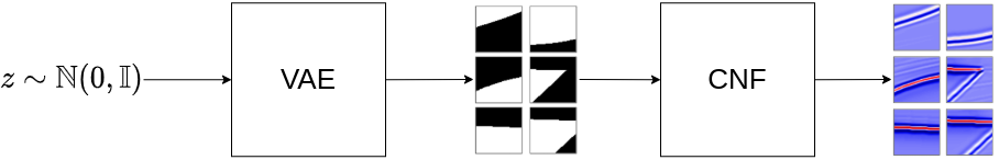
Figure 1: Data augmentation generation procedure.

The procedure is simple. First, we use the trained VAE model to sample salt masks $\hat{y}$, and then the image patches are sampled using $\hat{y}$ as conditional data.

In the following, we describe the setup, hyper-parameter settings, and learning procedure for the VAE and CNF models trained in this work.

Variational AutoEncoder

We train a simple VAE [15] model used to sample salt masks given to the CNF model as conditional data during the data augmentation generation procedure. The VAE encoder and decoder are just simple feed-forward networks. The encoder contains four stacked dense layers. In its turn, the decoder contains five stacked dense layers. Figure 2 illustrates the VAE architecture.

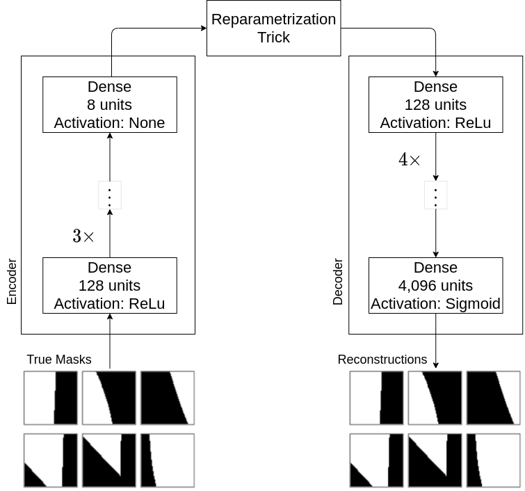
Figure 2: VAE layers composition.

Moreover, the model inputs are flattened, and the outputs are reshaped to form images.

Finally, the VAE model is trained via gradient descent with mini-batches of size $300$ to minimize the loss described by equation 1. Thus, the model is trained for $65.6K$ iterations using the Adam optimizer [47] with its default parameters, and the initial learning rate is $10^{-3}$. Additionally, the learning rate is scheduled to decay in a polynomial form, with a warm-up phase of $6.5K$ steps. The training procedure takes about $8$ hours and $13$ minutes on an NVidia Tesla P100 GPU, and the training loss converged around $31.54$.

Conditional Normalizing Flows

We train a CNF model, which, during the data augmentation generation procedure, receives the sampled masks $\hat{y}$ as inputs to generate the associated seismic image patches $\hat{x}$.

The CNF uses multi-scale architecture, with four scale levels and $15$ step-flow blocks per level. The Invertible $1\times 1$ Convolution outputs are given as inputs to the Affine Coupling Layer at each block, which has its backbone network illustrated in figure 3.

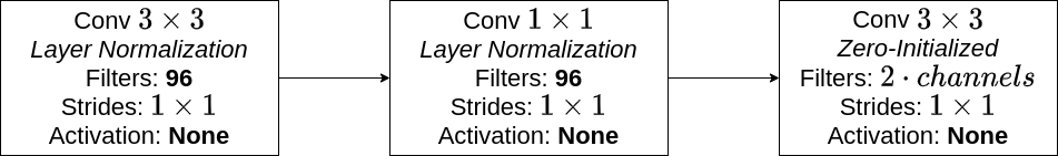
Figure 3: Coupling Layer’s backbone

All backbone weights are initialized by the Xavier Normal initialization method [48], except for the weights of the last convolutional layer, which is initialized with zeros.

In it turns, the Prior Network is composed of 4 stacked $3\times 3$ convolutions followed by a last zero-initialized $1\times 1$ convolutional layer. Figure 4 illustrates the prior network.

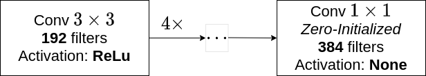
Figure 4: Prior Network.

Additionally, padding and strides are set such that each $3\times 3$ convolutional layer halves the inputs’ spatial dimension and the last $1\times 1$ convolutional layer doubles the $z$ channel dimensions with $384$ filters.

The model is trained to minimize the input data negative log-likelihood, calculated through equation 2. Moreover, during the training procedure, we regularize the model with the Binary Cross-Entropy loss to ensure spatial correlation between the learned latent space variables $z$ and the conditional data $y$. Such a regularization is analogous to the regularization proposed in the Glow paper [18], which penalizes the miss-classifications of a linear layer when learning a class-conditioned model.

To compute the Binary Cross-Entropy loss, we use an auxiliary network jointly trained with the whole CNF model. Such as in the Conditional Glow, this auxiliary network receives the latent variable $z$ as input and outputs the predicted respective mask. In summary, the auxiliary network comprises four stacked $3\times 3$ transposed convolutions [49], followed by a $3\times 3$ convolutional layer where each transposed convolution doubles the input’s spatial resolution. Figure 5 illustrates this auxiliary network.

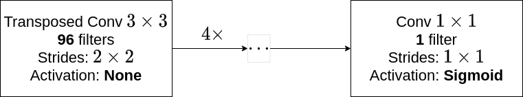
Figure 5: Auxiliary network, used to compute the regularization term during the training procedure.

Finally, the CNF model is trained on the training and validation sets, using the Adam Optimizer [47], with its default hyper-parameters, during $396.8K$ iterations and mini-batch size $50$. Polynomial decay is applied to the learning rate, which goes from $10^{-}4$ to $0$. The training procedure takes about four days on a Google Cloud TPU v2-8, and the training loss converges around $1.67$.

5 Dataset

We conduct extensive experiments on a dataset from two publicly available synthetic salt prospects models, and our results are presented on that dataset. The Pluto1.5 dataset [20], and the SEG/EAGE Salt model [21], are designed to emulate salt prospects in deep water, such as those found in the Gulf of Mexico.

We extract a 2D migrated image from each seismic model, and the binary salt mask is extracted from its velocity model by thresholding and clipping. Additionally, each migrated image is normalized by its mean and standard deviation.

We split the images into training, validation, and test sets. Figure 6 illustrates the migrated images, their respective binary masks, and our data splits.

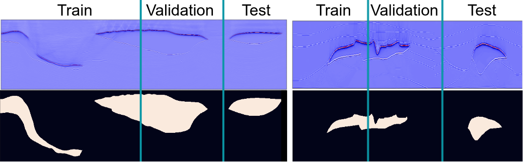
Figure 6: Seismic migrated images and their binary masks. The first row in the figure presents two entire seismic images, and the second row shows their corresponding salt masks. The black regions in the salt masks represent non-salt areas in their respective seismic images. The vertical bars in the image delimitate the locations of each image that are designated for the dataset’s train, validation, and test sets.

In our experiments, the images and masks, illustrated in figure 6, are processed into patches for training and evaluating the generative and semantic segmentation models. Moreover, we use distinct strategies for processing the seismic images and salt masks into patches due to the different goals of the generative and semantic segmentation models. In the following, we describe both procedures.

Patch Processing for the Generative Models

The goal of training the VAE and the CNF models is to generate pairs of seismic image patches and their respective salt masks that lie in the boundary of a salt body. With this proposal, the VAE and CNF models are trained using only patches which contain at least $10\%$ and a maximum of $90\%$ of salt.

Therefore, the seismic images train and validation, partitions are processed to create an overlapping grid of $64\times 64$ images and masks such that adjacent patches in the seismic image have $90\%$ overlap area. After it, patches that contain at least $10\%$ and a maximum of $90\%$ of salt are filtered and used as training examples. At last, the resulting data is augmented by horizontal flipping.

The resulting dataset comprises $24.872$ pairs of patches and binary masks containing different segments of a salt body boundary. Figure 7 shows examples of migrated image patches and their respective salt masks.

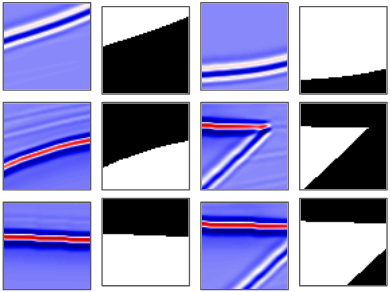
Figure 7: Examples of the migrated image patches and their respective salt masks. In the image, the second and fourth columns represent salt masks in which black regions represent non-salt areas. The first and third columns represent the respective seismic representation patches.

Patch Processing for the Semantic Segmentation Models

The semantic segmentation of salt bodies task consists of predicting binary salt masks that depict salt regions from the inputted seismic image patches. With the purpose of training and evaluating models for this task, the dataset training, validation, and test sets are processed to create an overlapping grid of $64\times 64$ patches. The overlapping grid is created such that adjacent patches in the image partition have $10\%$ overlap, and there are no overlapping partitions. At last, the data is augmented by horizontal flipping each resulting sample pair.

The resulting dataset comprises $6,000$ sample pairs, distributed as follows: $2.450$ samples for the training set; $1.434$ samples for the validation set; and $2.042$ samples for the test set.

Finally, it is important to note that all image patches are used to create the dataset, unlike the previous procedure where only the patches on a salt body border are taken.

6 Experiments

In this section, we present our experiments and the achieved results. The IoU (Intersection Over Union) metric at a $0.5$ threshold evaluates the model’s performance, such as proposed in the PASCAL VOC challenge [50].

6.1 Augmentations Effects

This experiment aims to determine how many generated pairs of salt masks and image patches should be used to augment the dataset while training models for the semantic segmentation of salt bodies. Thus, we train several U-net models [22] exploring different values for the augmentation size hyper-parameter, which controls how many generated sample pairs are used as data augmentation. The data augmentation samples are generated by the method and models described in 4.

In summary, the experiment consists of evaluating the IoU metric on the dataset’s training and validation sets for models trained with different values for the augmentation size, from $0$ to $700$. We train ten U-net models at each iteration, with varying augmentation samples – i.e. pairs of seismic image patches and salt masks. Subsequently, the IoU metric is evaluated in training set for each model. Then the model with the second-best training metric is selected, and the other nine models are discarded. The iteration finishes by evaluating the selected model on the validation set.

We observe that it is required to test some distinct generated augmentation sets for achieving good results due to the high level of noise and bias added by our DA method. We found that five or fewer trials are usually sufficient for finding such an augmentation set, but we maintained ten shots to ensure consistency. It is important to note that we select the second-best training metric to avoid selecting highly over-fitted models.

All models are trained with the U-net implementation provided by [51] for $60$ epochs, using the Adam optimizer [47] with default hyperparameters, and the learning rate equals $10^{-3}$. Additionally, the models have four encoder and decoder blocks, and the first block has $65$ filters for its convolutional layers. The number of filters is doubled at each block, and the whole model has $7.69M$ trainable parameters. The training procedure takes an average time of 10 minutes per model on a Tesla P100 graphic processing unit (GPU).

In total, we train $80$ U-Net models, but we only report the metrics for the eight selected models. Figure 8 presents the training and validation performance curve for the selected models at different sizes of augmentations, ranging from $0$ to $700$.

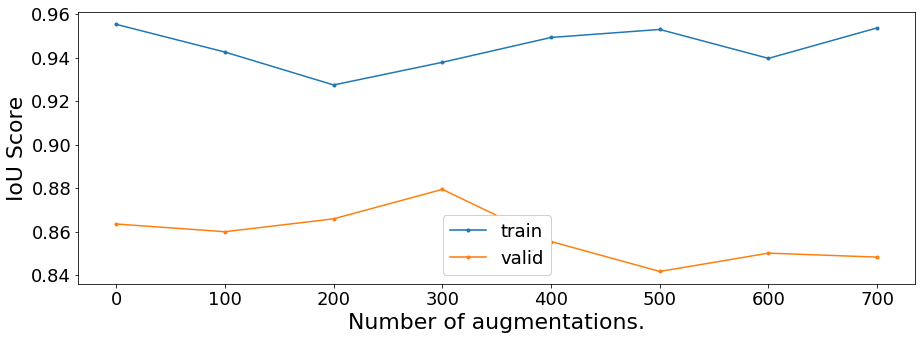
Figure 8: IoU per number of augmentations.

Among the different augmentation sizes, the model trained without augmentations is the one that has the highest IoU score on the training set. Then, up to $200$ augmentations, the training score decays from $.96$ to $.92$, which is the lowest. From this point, the training metric rises practically back to the initial level.

On the other hand, we observe an increasing validation score until we achieve $300$ augmentations, which presents the highest validation score. From $400$ onwards, the validation IoU quickly degenerates while we observe a rising training score, indicating that the model starts to overfit the augmentations from this point.

Moreover, observing the decay in the training metric while observing the growth in the validation metric may indicate that the data augmentations regularize the model during training, thus avoiding overfit and improving its generalization. Also, the highest validation metric is achieved by the model with the second-lowest training score. It is observed in an inflection point, from where the validation metrics start to degenerate while the training score still increases. It may indicate that at $300$ augmentations, the model achieves a good balance between regularization and overfitting.

6.2 Performance Comparison

This section compares the performance of distinct models when trained using and not using our generated augmentation samples, aiming to show that our proposed method results in gains independently on the models’ architecture and the number of parameters. For this purpose, we compare the performance of the U-Net against seven variants of the DeeplabV3+ model [23]. The DeeplabV3+ was chosen because its official implementation provides, out-of-the-shelf, several changeable backbone architectures with different depths and number of parameters. Three widely used architectures are explored as backbone: Xception [52]; MobileNet [53]; Resnet [33];

The U-net model is trained with the same configuration as explained in section 6.1, and all DeeplabV3+ models are trained using the official implementation . Models with the Xception and ResNet backbones have the Atrous rate, output stride, and decoder output stride hyper-parameters set respectively to $[12,24,36]$, $8$, and $4$. Moreover, all models with the MobileNet (V2 and V3) backbones, the Atrous rates, and output stride hyper-parameters are left empty. In models with the MobileNetV3 backbone, the decoder output stride hyper-parameter is set to 8. We provide more detailed hyper-parameter settings for each model on the supplementary material accompanying this paper.

Finally, for comparison purposes, all models are trained using the Adam Optimizer for $40K$ training iterations and a mini-batch of $20$ examples per iteration on an NVidia Tesla P100 graphic processing unit (GPU).

Table 1 present the number of trainable parameters and the obtained results in the validation and test sets for each model when trained with and without the proposed DA method. The augmented versions are trained with the addition of $300$ generated pairs of salt masks and image patches.

Table 1: Performance comparison between models trained with and without data augmentation.

Model	Backbone	Trainable Parameters	Not Augmented		Augmented
			$Validation$ (%)	$Test$ (%)	$Validation$ (%)	$Test$ (%)
U-net	-	$7,69M$	88.66	93.03	88.57	94.71
DeepLab	mobilenet_v2	$2.10M$	81.12	82.83	90.02	86.83
	mobilenet_v3_small	$.82M$	66.23	71.90	83.52	88.76
	mobilenet_v3_large	$1.91M$	73.82	82.34	78.04	89.83
	xception_41	$28.10M$	77.45	75.35	88.69	81.94
	xception_65	$41.05M$	82.34	85.14	77.12	90.11
	xception_71	$41.60M$	62.99	61.86	77.42	77.39
	resnet_v1_18	$12.33M$	89.15	93.75	89.68	95.17
	resnet_v1_50	$26.69M$	87.66	88.92	85.96	91.77
	resnet_v1_101	$45.68M$	89.16	93.17	91.08	95.17

The proposed data augmentation method yields consistent improvements for all models in the IoU metric. On average, we find a gain of $8.57\%$ in the test metric. The best improvement is $25.10\%$, found with the DeeplabV3+ using the xception_71 backbone. Also, the best result is achieved with the augmented dataset by the resnet_v1_101 backbone. This model reaches $95.17\%$ in the test score, which corresponds to an improvement of $2.14\%$. Interestingly, the models with the xception_65 and resnet_v1_50 backbones and the U-net model present a slight reduction in their validation metric, indicating that somehow the augmentation regularized those models, helping to improve their generalization on unseen data.

6.3 Comparison against other Data Augmentation methods

We compare the performance of the proposed DA method against seven distinct methods from the Albumentation library [54]. Thus, the performance of the DeeplabV3+ with the mobilenet_v3_large backbone is evaluated for models trained using the following methods: Elastic Transform; Grid Distortion; Optical Distortion; CLAHE; Random Brightness Contrast; Random Gamma. Those methods were selected because they have shown noticeable results for medical and image applications [55, 56, 57, 58]. Additionally, we also evaluate the models’ performance when composing our proposed DAs together with the transformations enumerated above. It is important to note that only the original samples are passed through the transformations. Therefore, our DA samples are only presented to the models without being passed through any transformation.

All models are trained using the same settings described in section 6.2 and took an average time of $1$ hour and $10$ minutes on an Nvidia Tesla P100 GPU.

Table 2 compares the obtained results, in the validation and test sets, of each Albumentation method against our proposed data augmentation and the composition of both methods.

Table 2: Performance comparison between data augmentation methods against our proposed augmentations. In the center columns, we present the results achieved when each DA method stand-alone. In the right columns, we present the results achieved when composing each method with our proposed DA.

Method	Alone		+ Ours
	Validation (%)	Test (%)	Validation (%)	Test (%)
None	73.82	82.34	-	-
Ours	78.04	89.83	-	-
ElasticTransform	86.56	89.09	75.88	90.39
CLAHE	81.15	89.78	78.40	86.67
Grid Distortion	77.99	85.72	87.19	89.60
Random Gamma	86.31	87.31	86.51	83.59
Random Brightness Contrast	80.39	82.25	76.91	86.33
Optical Distortion	68.06	74.90	84.26	82.21

Comparing the obtained results for the models trained with a single DA method (the center column), we observe that our method achieves the best result. Moreover, except for the Random Brightness Contrast and Optical Distortion methods, all methods improve both the validation and test sets. The highest test score, $90.39\%$, is achieved when applying the Elastic Transform and our DAs together. Also, composing our DAs with the Optical Distortion, Random Brightness Contrast, and Grid Distortion methods result in better generalization than when applying those methods alone. Such results may indicate that our approach could complement other DA methods, improving the models’ performance even more. On the other hand, it is not all methods that improve results when applied with our DAs together. The CLAHE and Random Gamma methods present better results when used alone. Unfortunately, we could not identify an apparent reason for these results.

6.4 Performance comparison on a larger context size

In this experiment, we compare the performance of the DeeplabV3+ using the mobilenet_v3_large backbone when trained using and not using our generated DAs for $128\times 128$ patches aiming to demonstrate that our proposal also works with larger context sizes, i.e., larger patch sizes. For this purpose, we train the generative models, with the same setup described in section 4, for $128\times 128$ context size. The context patches are processed to create an overlapping grid of $128\times 128$ with $90\%$ overlap between adjacent patches. Additionally, only the patch samples containing between $10\%$ and $90\%$ of salt are used. The data is also augmented by applying horizontal flips, resulting in $11.056$ samples.

The CNF model achieves a loss value of $1.81$ after six days and $259,2K$ training iterations on a Google Cloud TPU v2-8. In its turn, the VAE loss converged around $61.17$ after $14$ hours and $28.8K$ training iterations on an NVidia Tesla P100 GPU.

For the semantic segmentation model, $128\times 128$ context patches, with $10\%$ overlap between adjacent patches, are created, and the data is also augmented by applying horizontal flips. The resulting dataset contains $1,476$ samples, with $608$ in the training set, $356$ in the validation set, and $512$ in the test set. The DeeplabV3+ is trained during 40k iterations three times for augmented and not augmented versions, taking an average time of $6$ hours and $20$ minutes per model. Table 3 compares the performance of the model with the best validation score of each version.

Table 3: Performance comparison of the DeeplabV3+ model with the mobilenet_v3_large backbone for context size of $128\times 128$ when trained with and without data augmentation.

Version	$Validation$ (%)	$Test$ (%)
Not Augmented	74.09	84.85
Augmented	86.19	90.55

The augmented version improved the metrics on the validation and test sets from $74.09\%$ to $86.19\%$ and from $84.85\%$ to $90.55\%$, respectively. When compared against the results for the same model architecture, from experiment 6.2 (in $64\times 64$ contexts), the augmented and not augmented models outperformed their respective versions. Moreover, comparing the improvement percentage in the test set of the models trained for $64\times 64$ contexts against the models trained for $128\times 128$ contexts, we observe that although the percentage reduced from $9.09\%$, to $6.71\%$, we still have a significant gain when training the model with our proposed DA. We believe that the obtained results show the potential of the proposed DA method on larger context sizes. Finally, it is important to note that further investigation into context sizes has become prohibitive in this work due to the many executed experiments and the high computational cost required for this.

7 Conclusion

This work proposes a Data Augmentation (DA) method for the semantic segmentation of salt bodies in a seismic image dataset built from two public available synthetic salt models.

The performance of distinct state-of-the-art semantic segmentation models is compared when using and not using the proposed DAs during the training procedure. The proposed method yields consistent improvements independently from the model architecture or their number of trainable parameters. Moreover, our DA method achieves an average improvement of $8.57\%$ in the IoU metric. The best improvement, of $25.10\%$, is achieved by the DeeplabV3+ using the the xception_71 backbone. In it turns, the best result is achieved when augmenting data for the DeeplabV3+ with the resnet_v1_101 backbone. This model reaches $95.17\%$ in the test score, which corresponds to an improvement of $2.14\%$.

We also show that our proposal outperforms seven selected DA methods when they are applied stand-alone. Furthermore, by applying our data augmentations in composition with the ElastTransform augmentation method, DeeplabV3+ using the large version of the MobileNetV3 backbone achieves a $90.39\%$ score, which is the highest for this architecture. At last, the same methodology for $128\times 128$ context patches is applied, achieving results comparable to the obtained for smaller contexts, showing that our proposal is adaptable for larger contexts.

Future work could include testing the proposed method in other datasets, such as the one used in the TGS Salt Identification Challenge; application in other seismic tasks like the seismic facies segmentation [10, 8, 11]; adapting the methodology for natural images; and exploring the use of other generative models such as the Conditional GAN [59].

Finally, our experimental results show that the proposed DA method yields consistent improvements for different models and context sizes, helping develop models for the semantic segmentation of salt bodies.

References

- [1] Samuel H. Gray. 4. Seismic imaging, pages S1–1–S1–16. Society of Exploration Geophysicists, 2016.
- [2] Yauhen Babakhin, Artsiom Sanakoyeu, and Hirotoshi Kitamura. Semi-supervised segmentation of salt bodies in seismic images using an ensemble of convolutional neural networks. In Gernot A. Fink, Simone Frintrop, and Xiaoyi Jiang, editors, Pattern Recognition, pages 218–231, Cham, 2019. Springer International Publishing.
- [3] I. Jones and I. Davison. Seismic imaging in and around salt bodies. Interpretation, 2, 2014.
- [4] Jatin Bedi and Durga Toshniwal. Sfa-gtm: Seismic facies analysis based on generative topographic map and rbf. ArXiv, abs/1806.00193, 2018.
- [5] H. Di, M. Shafiq, and G. AlRegib. Multi-attribute k-means clustering for salt-boundary delineation from three-dimensional seismic data. Geophysical Journal International, 215:1999–2007, 2018.
- [6] T. Hegazy and Ghasssan AlRegib. Texture attributes for detecting salt bodies in seismic data. Seg Technical Program Expanded Abstracts, 2014.
- [7] Ioannis Pitas and Constantine Kotropoulos. A texture-based approach to the segmentation of seismic images. Pattern Recognit., 25:929–945, 1992.
- [8] Thilo Wrona, I. Pan, R. Gawthorpe, and H. Fossen. Seismic facies analysis using machine learning. Geophysics, 83, 2018.
- [9] X. Wu. Methods to compute salt likelihoods and extract salt boundaries from 3d seismic images. Geophysics, 81, 2016.
- [10] T. Zhao, V. Jayaram, A. Roy, and K. Marfurt. A comparison of classification techniques for seismic facies recognition. Interpretation, 3, 2015.
- [11] J. Dramsch and M. Lüthje. Deep-learning seismic facies on state-of-the-art cnn architectures. Seg Technical Program Expanded Abstracts, 2018.
- [12] A. U. Waldeland, A. Jensen, L. Gelius, and A. Solberg. Convolutional neural networks for automated seismic interpretation. Geophysics, 37:529–537, 2018.
- [13] Wenlong Wang, Fangshu Yang, and J Ma. Automatic salt detection with machine learning. In 80th EAGE Conference and Exhibition 2018, volume 2018, pages 1–5. European Association of Geoscientists & Engineers, 2018.
- [14] Yu Zeng, Kebei Jiang, and Jie Chen. Automatic seismic salt interpretation with deep convolutional neural networks. In Proceedings of the 2019 3rd International Conference on Information System and Data Mining, ICISDM 2019, page 16–20, New York, NY, USA, 2019. Association for Computing Machinery.
- [15] Diederik P. Kingma and Max Welling. Auto-encoding variational bayes. CoRR, abs/1312.6114, 2013.
- [16] Laurent Dinh, David Krueger, and Yoshua Bengio. Nice: Non-linear independent components estimation. CoRR, abs/1410.8516, 2014.
- [17] Laurent Dinh, Jascha Sohl-Dickstein, and Samy Bengio. Density estimation using real nvp. ArXiv, abs/1605.08803, 2016.
- [18] Diederik P. Kingma and Prafulla Dhariwal. Glow: Generative flow with invertible 1x1 convolutions. In NeurIPS, 2018.
- [19] Lynton Ardizzone, Carsten Lüth, Jakob Kruse, Carsten Rother, and Ullrich Köthe. Guided image generation with conditional invertible neural networks. ArXiv, abs/1907.02392, 2019.
- [20] D. Stoughton, J. Stefani, and S. Michell. 2d elastic model for wavefield investigations of subsalt objectives, deep water gulf of mexico. Seg Technical Program Expanded Abstracts, 2001.
- [21] F. Aminzadeh, N. Burkhard, T. Kunz, L. Nicoletis, and F. Rocca. 3-d modeling project: 3rd report. Geophysics, 14:125–128, 1995.
- [22] Olaf Ronneberger, Philipp Fischer, and Thomas Brox. U-net: Convolutional networks for biomedical image segmentation. ArXiv, abs/1505.04597, 2015.
- [23] Liang-Chieh Chen, Yukun Zhu, George Papandreou, Florian Schroff, and Hartwig Adam. Encoder-decoder with atrous separable convolution for semantic image segmentation. In ECCV, 2018.
- [24] M. Shafiq, Zhen Wang, Asjad Amin, T. Hegazy, Mohamed Deriche, and G. AlRegib. Detection of salt-dome boundary surfaces in migrated seismic volumes using gradient of textures. Seg Technical Program Expanded Abstracts, 2015.
- [25] M. Shafiq, Tariq A. Alshawi, Z. Long, and G. Al-Regib. Salsi: A new seismic attribute for salt dome detection. 2016 IEEE International Conference on Acoustics, Speech and Signal Processing (ICASSP), pages 1876–1880, 2016.
- [26] Amin Asjad and Deriche Mohamed. A new approach for salt dome detection using a 3d multidirectional edge detector. Applied Geophysics, 12:334–342, 2015.
- [27] Bowen Cheng, Maxwell D. Collins, Y. Zhu, T. Liu, T. Huang, H. Adam, and Liang-Chieh Chen. Panoptic-deeplab: A simple, strong, and fast baseline for bottom-up panoptic segmentation. 2020 IEEE/CVF Conference on Computer Vision and Pattern Recognition (CVPR), pages 12472–12482, 2020.
- [28] Yi Zhu, Karan Sapra, F. Reda, Kevin J. Shih, S. Newsam, A. Tao, and Bryan Catanzaro. Improving semantic segmentation via video propagation and label relaxation. 2019 IEEE/CVF Conference on Computer Vision and Pattern Recognition (CVPR), pages 8848–8857, 2019.
- [29] H. Di, Z. Wang, and G. AlRegib. Real-time seismic-image interpretation via deconvolutional neural network. Seg Technical Program Expanded Abstracts, 2018.
- [30] Netherlands F3 Dataset. https://terranubis.com/datainfo/F3-Demo-2020. Accessed: 2021-06-04.
- [31] H. Di, Zhen Wang, and G. AlRegib. Deep convolutional neural networks for seismic salt-body delineation*. In AAPG Annual Convention and Exhibition 2018, 2018.
- [32] Kaiming He, Xiangyu Zhang, Shaoqing Ren, and Jian Sun. Identity mappings in deep residual networks. ArXiv, abs/1603.05027, 2016.
- [33] Kaiming He, Xiangyu Zhang, Shaoqing Ren, and Jian Sun. Deep residual learning for image recognition. 2016 IEEE Conference on Computer Vision and Pattern Recognition (CVPR), pages 770–778, 2016.
- [34] SEAM Open Data. https://seg.org/News-Resources/Research-Data/Open-Data. Accessed: 2021-06-04.
- [35] Djork-Arné Clevert, Thomas Unterthiner, and S. Hochreiter. Fast and accurate deep network learning by exponential linear units (elus). arXiv: Learning, 2016.
- [36] A. Rakhlin, A. Davydow, and S. Nikolenko. Land cover classification from satellite imagery with u-net and lovász-softmax loss. 2018 IEEE/CVF Conference on Computer Vision and Pattern Recognition Workshops (CVPRW), pages 257–2574, 2018.
- [37] Yunzhi Shi, X. Wu, and S. Fomel. Saltseg: Automatic 3d salt segmentation using a deep convolutional neural network. Interpretation, 7, 2019.
- [38] X. Wu, Luming Liang, Yunzhi Shi, and S. Fomel. Faultseg3d: Using synthetic datasets to train an end-to-end convolutional neural network for 3d seismic fault segmentation. Geophysics, 84, 2019.
- [39] Aleksandar Milosavljevic. Identification of salt deposits on seismic images using deep learning method for semantic segmentation. ISPRS Int. J. Geo Inf., 9:24, 2020.
- [40] Gao Huang, Zhuang Liu, and Kilian Q. Weinberger. Densely connected convolutional networks. 2017 IEEE Conference on Computer Vision and Pattern Recognition (CVPR), pages 2261–2269, 2017.
- [41] Michael I. Jordan, Zoubin Ghahramani, T. Jaakkola, and L. Saul. An introduction to variational methods for graphical models. Machine Learning, 37:183–233, 1999.
- [42] Danilo Jimenez Rezende, Shakir Mohamed, and Daan Wierstra. Stochastic backpropagation and approximate inference in deep generative models. In ICML, 2014.
- [43] C. Winkler, Daniel Worrall, E. Hoogeboom, and M. Welling. Learning likelihoods with conditional normalizing flows. ArXiv, abs/1912.00042, 2019.
- [44] Andreas Lugmayr, Martin Danelljan, L. Gool, and R. Timofte. Srflow: Learning the super-resolution space with normalizing flow. ArXiv, abs/2006.14200, 2020.
- [45] Ruslan Salakhutdinov and Geoffrey E. Hinton. Deep boltzmann machines. In AISTATS, 2009.
- [46] Chen-Yu Lee, Saining Xie, Patrick W. Gallagher, Zhengyou Zhang, and Zhuowen Tu. Deeply-supervised nets. ArXiv, abs/1409.5185, 2014.
- [47] Diederik P. Kingma and Jimmy Ba. Adam: A method for stochastic optimization. CoRR, abs/1412.6980, 2014.
- [48] Xavier Glorot and Yoshua Bengio. Understanding the difficulty of training deep feedforward neural networks. In AISTATS, 2010.
- [49] Matthew D. Zeiler, Dilip Krishnan, Graham W. Taylor, and Rob Fergus. Deconvolutional networks. 2010 IEEE Computer Society Conference on Computer Vision and Pattern Recognition, pages 2528–2535, 2010.
- [50] M. Everingham, L. Gool, C. K. Williams, J. Winn, and Andrew Zisserman. The pascal visual object classes (voc) challenge. International Journal of Computer Vision, 88:303–338, 2009.
- [51] Joel Akeret, Chihway Chang, Aurelien Lucchi, and Alexandre Refregier. Radio frequency interference mitigation using deep convolutional neural networks. Astronomy and Computing, 18:35–39, 2017.
- [52] François Chollet. Xception: Deep learning with depthwise separable convolutions. 2017 IEEE Conference on Computer Vision and Pattern Recognition (CVPR), pages 1800–1807, 2016.
- [53] Andrew Howard, Mark Sandler, Grace Chu, Liang-Chieh Chen, Bo Chen, Mingxing Tan, Weijun Wang, Yukun Zhu, Ruoming Pang, Vijay Vasudevan, Quoc V. Le, and Hartwig Adam. Searching for mobilenetv3. In ICCV, 2019.
- [54] Alexander Buslaev, Vladimir I. Iglovikov, Eugene Khvedchenya, Alex Parinov, Mikhail Druzhinin, and Alexandr A. Kalinin. Albumentations: Fast and flexible image augmentations. Information, 11(2), 2020.
- [55] P.Y. Simard, D. Steinkraus, and J.C. Platt. Best practices for convolutional neural networks applied to visual document analysis. In Seventh International Conference on Document Analysis and Recognition, 2003. Proceedings., pages 958–963, 2003.
- [56] Eduardo Castro, Jaime S. Cardoso, and J. C. Pereira. Elastic deformations for data augmentation in breast cancer mass detection. 2018 IEEE EMBS International Conference on Biomedical & Health Informatics (BHI), pages 230–234, 2018.
- [57] Hai Huang, Hao Zhou, Xu Yang, Lu Zhang, Lu Qi, and Ai-Yun Zang. Faster r-cnn for marine organisms detection and recognition using data augmentation. Neurocomputing, 337:372–384, 2019.
- [58] Tinuk Agustin, Ema Utami, and Hanif Al Fatta. Implementation of data augmentation to improve performance cnn method for detecting diabetic retinopathy. In 2020 3rd International Conference on Information and Communications Technology (ICOIACT), pages 83–88. IEEE, 2020.
- [59] Mehdi Mirza and Simon Osindero. Conditional generative adversarial nets. ArXiv, abs/1411.1784, 2014.