Geometry of shallow-water dynamics with thermodynamics

Abstract

We review the geometric structure of the IL⁰PE model, a rotating shallow-water model with variable buoyancy, thus sometimes called “thermal” shallow-water model. We start by discussing the Euler–Poincaré equations for rigid body dynamics and the generalized Hamiltonian structure of the system. We then reveal similar geometric structure for the IL⁰PE. We show, in particular, that the model equations and its (Lie–Poisson) Hamiltonian structure can be deduced from Morrison and Greene’s (1980) system upon ignoring the magnetic field ($\vec{\mathrm{B}}=0$) and setting $U(\rho,s)=\frac{1}{2}\rho s$, where $\rho$ is mass density and $s$ is entropy per unit mass. These variables play the role of layer thickness ($h$) and buoyancy ($\bar{\vartheta}$) in the IL⁰PE, respectively. Included in an appendix is an explicit proof of the Jacobi identity satisfied by the Poisson bracket of the system.

1 Introduction

Following notation introduced by Ripa,²¹ IL⁰PE stands for inhomogeneous-layer primitive-equation(s) with the superscript indicating that buoyancy does not vary in the vertical, while it is allowed to unrestrainedly vary in horizontal position and time. The IL⁰PE has the two-dimensional structure of a rotating shallow-water model with an additional evolution equation for the buoyancy. This model was extensively used through the 1980s and 1990s ¹¹, ²⁶, ¹², ¹ to investigate mixed-layer (upper ocean) dynamics as it allows one to accommodate, in a two-dimensional setting and thus more easily, heat and freshwater fluxes through the ocean’s surface. Such “thermal shallow-water” modeling was abandoned due in large part to the increase of computational power and a preference—I dare to say—to emphasize reproducing observations over understanding the basic aspects of the dynamics. However, a gratifying surprise has been to learn that this type of modelling is regaining momentum,²⁸, ⁷ particularly for the ability of the model to produce small-scale circulations similar to those observed in ocean color images, even at low frequency (Fig. 1). This renewed interest motivated investigating the geometric properties of the system further,³, ² following pioneering work by Ripa.²⁰, ²¹, ²², ²⁴ We review those properties here and also establish an explicit connection, so far overlooked, with seminal work by Morrison and Greene ¹⁶ on generalized Hamiltonians. The exposition starts by reviewing similar geometric structure for rigid-body dynamics. We also include an explicit proof in an appendix of the Jacobi identity that the Poisson bracket of the model equations must satisfy.

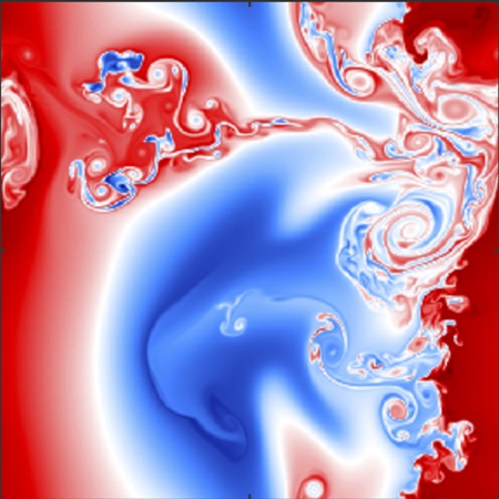
Figure 1: Snapshot of potential vorticity from a numerical solution of a quasigeostrophic version of the IL⁰PE model (15)–(17) in a doubly periodic domain $[0,1]\times[0,1]$. Note the Kelvin–Helmholtz-like rollup filaments (length is scaled by the deformation radius of the system).

2 Background: The rigid body

The free rigid body (Euler) equations in principle axis coordinates are

$$\mathbb{I}\dot{\boldsymbol{\Omega}}=\mathbb{I}\boldsymbol{\Omega}\times\boldsymbol{\Omega}$$ (1)

where $\mathbb{I}$ is the (diagonal) tensor of inertia and $\boldsymbol{\Omega}(t)$ is the angular velocity of the body.

2.1 Euler–Poincaré equations

These equations follow from the variational principle

$$\delta\int_{t_{0}}^{t_{1}}L(\boldsymbol{\Omega})\operatorname{d}\!{t}=0,\quad L(\boldsymbol{\Omega}):=\tfrac{1}{2}\mathbb{I}\boldsymbol{\Omega}\cdot\boldsymbol{\Omega}$$ (2)

with constrained variations

$$\delta\boldsymbol{\Omega}=\dot{\boldsymbol{\Sigma}}+\boldsymbol{\Sigma}\times\boldsymbol{\Omega}$$ (3)

for some vector $\boldsymbol{\Sigma}(t)$ such that it vanishes at the endpoints. The function $L(\boldsymbol{\Omega})$ is the Lagrangian. The resulting equations

$$\frac{\operatorname{d}\!{}}{\operatorname{d}\!{t}}{}\frac{\partial L}{\partial\boldsymbol{\Omega}}=\frac{\partial L}{\partial\boldsymbol{\Omega}}\times\boldsymbol{\Omega}$$ (4)

are known as the Euler–Poincaré equations.¹⁰

2.2 Generalized Hamiltonian structure

Using the angular momentum $\mathbf{M}:=\mathbb{I}\boldsymbol{\Omega}$, system (1) reads

$$\dot{\mathbf{M}}=\mathbf{M}\times\mathbb{I}^{-1}\mathbf{M}.$$ (5)

This set can be obtained by the Legendre transform $\boldsymbol{\Omega}\mapsto\mathbf{M}$ defined by

$$H(\mathbf{M})=\mathbf{M}\cdot\boldsymbol{\Omega}-L(\boldsymbol{\Omega})$$ (6)

and the Poisson tensor $\mathbb{J}$ with components

$$\mathbb{J}^{ij}=\varepsilon^{ij}_{k}M^{k}$$ (7)

according to

$$\dot{\mathbf{M}}=\mathbb{J}\nabla H(\mathbf{M}),$$ (8)

which provides a generalized Hamiltonian ²⁵, ²⁷, Ripa-RMF-92, ¹⁵ formulation for the rigid body. The function $H(\mathbf{M})$ is the Hamiltonian. Associated with $\mathbb{J}$ is the Poisson bracket, defined and given by

$$\{U,V\}:=\nabla U(\mathbf{M})\cdot\mathbb{J}\nabla V(\mathbf{M})=-\mathbf{M}\cdot\nabla U(\mathbf{M})\times\nabla V(\mathbf{M}).$$ (9)

This bracket is of the Lie–Poisson type, i.e, linear in the phase space coordinate $\mathbf{M}$, and (thus) satisfies

$$\{U,V\}=-\{V,U\}\quad\text{(antisymmetry)}, \{U,\{V,W\}\}+\operatorname{\circlearrowleft}=0\quad\text{(Jacobi identity)}.$$ (10)

2.2.1 Casimirs

The Hamiltonian (energy) is an integral of motion, clearly since $\dot{H}=\{H,H\}\equiv 0$. But the dynamics are constrained by additional conservation laws. More precisely, because $\det\mathbb{J}=0$, i.e., $\mathbb{J}$ is singular, there exist functions $C(\mathbf{M})$, called Casimirs (Lie’s distinguished functions), whose gradients span the null space of $\mathbb{J}$, namely, they satisfy

$$\mathbb{J}\nabla C(\mathbf{M})=0.$$ (11)

These are given by

$$C(\mathbf{M})=F(\tfrac{1}{2}|\mathbf{M}|^{2})\quad\forall F(\,).$$ (12)

Note that $C(\mathbf{M})$ commutes with any function of state in the Poisson bracket, viz.,

$$\{U,C\}=0\quad\forall U(\mathbf{M});$$ (13)

hence, they are conserved under the dynamics: $\dot{C}=\{C,H\}\equiv 0$. Note that the equations of motion are not altered under the change of Hamiltonian $H\mapsto H+\lambda C$, $\lambda=\operatorname{const}$. The extremal points of $H$, however, may be altered under this change.

2.2.2 Geometry

More generally, let $z(t)$ represent a point in a space $M$ equipped with a Poisson bracket $\{\,,\hskip 1.00006pt\}$. One calls the pair $(M,\{\,,\hskip 1.00006pt\})$ a Poisson manifold. The dynamical system $\dot{z}=\mathbb{J}\nabla H(z)=\{z,H\}$ represents a (generalized) Hamiltonian system. More broadly, $\dot{F}=\{F,H\}$ for any function of state $F(z)$. If the Poisson tensor (matrix) is singular, then $\operatorname{dim}M=m$ must necessarily be odd. This is different than canonical Hamiltonian dynamics for which $\operatorname{dim}M=2n$. Indeed, in such a case $z=(q,p)$, which satisfy $\dot{q}=+\partial_{p}H$ and $\dot{p}=-\partial_{q}H$. Thus

$$\mathbb{J}=\begin{pmatrix}0&+\operatorname{Id}^{n\times n}\\ -\operatorname{Id}^{n\times n}&0\end{pmatrix},\quad\det\mathbb{J}=1,$$ (14)

which is called symplectic matrix. It turns out that an $m$-dimensional manifold is generically foliated by $2n$-dimensional surfaces $\{C=\operatorname{const}\}$, called symplectic leaves, on which the dynamics is canonical (clearly, if $z(0)$ lies on $\{C=\operatorname{const}\}$, $z(t)$ will remain there for all $t$).

2.2.3 Noether’s theorem

Finally, Noether’s theorem relates symmetries with conservation laws. Energy is related with symmetry under $t$ shifts and $s$-momentum with $s$-translational symmetry. Casimirs are not associated with explicit symmetries, but rather with symmetries lost in the process of reducing a canonical Hamiltonian system to a generalized (i.e., singular) Hamiltonian system. For instance, a canonical system with dimension, say, $2n=4$, that has one integral of motion $I$ (say) can be reduced to a singular system with dimension $m=3$ when it is constrained to the manifold $\{I=\operatorname{const}\}$. Such a loss of explicit symmetries happens in fluid systems when formulated in Eulerian variables: the Casimirs of hydrodynamics are related to the symmetry of the Eulerian variables under Lagrangian particle relabelling,¹⁷, ¹⁹, ¹⁸ yet with a possibly important caveat.⁵

3 The IL⁰PE model

The IL⁰PE model in some closed domain $D$ of the $\beta$ plane in a reduced-gravity setting is given by (e.g., Ripa ²²)

$$\partial_{t}\bar{\mathbf{u}}+(\bar{\mathbf{u}}\cdot\nabla)\bar{\mathbf{u}}+f\hat{\mathbf{z}}\times\bar{\mathbf{u}}+\tfrac{1}{2}h^{-1}\nabla h^{2}\bar{\vartheta} =0,$$ (15)

$$\partial_{t}h+\nabla\cdot h\bar{\mathbf{u}} =0,$$ (16)

$$\partial_{t}\bar{\vartheta}+\bar{\mathbf{u}}\cdot\nabla\bar{\vartheta} =0,$$ (17)

where velocity $(\bar{\mathbf{u}})$, layer thickness ($h$) and buoyancy ($\bar{\vartheta}$) are functions of horizontal position $(\mathbf{x})$ and time ($t$). Appropriate boundary conditions are

$$\bar{\mathbf{u}}\cdot\hat{\mathbf{n}}=0,\quad\hat{\mathbf{n}}\times\nabla\bar{\vartheta}=0\quad(\mathbf{x}\in\partial D).$$ (18)

The condition on the left simply means no flow through the boundary of $D$; the condition on the right (viz., that the boundary is isopycnic) is needed to convey the IL⁰PE a generalized Hamiltonian structure.

Remark 1

The parenthesis in $(\mathbf{a}\cdot\nabla)\mathbf{b}$ is not superfluous! Indeed,

$$\mathbf{a}\cdot\nabla\mathbf{b}=\mathbf{a}^{\top}\nabla\mathbf{b}=(\nabla\mathbf{b})^{\top}\mathbf{a}=(\nabla\mathbf{b})\cdot\mathbf{a}=a_{j}\nabla b_{j}$$ (19)

while

$$(\mathbf{a}\cdot\nabla)\mathbf{b}=(\nabla\mathbf{b})\mathbf{a}=a_{j}\partial_{j}\mathbf{b}$$ (20)

(assuming that vectors are column and $\nabla\mathbf{a}$ is a matrix with rows given by $\nabla a_{i}$).

Remark 2

The set $\{\bar{\vartheta}=g^{\prime}=\operatorname{const}\}$ is an invariant manifold of the IL⁰PE on which the dynamics are controlled by the HLPE, viz., $\partial_{t}\bar{\mathbf{u}}+(\bar{\mathbf{u}}\cdot\nabla)\bar{\mathbf{u}}+f\hat{\mathbf{z}}\times\bar{\mathbf{u}}+g^{\prime}\nabla h=0$ and $\partial_{t}h+\nabla\cdot h\bar{\mathbf{u}}=0$.

For the purpose of revealing the geometric structure of the IL⁰PE, it is convenient to write the momentum equation (15) in two different but equivalent forms:

$$\frac{\operatorname{D}\!{}}{\operatorname{D}\!{t}}(\bar{\mathbf{u}}+\mathbf{f})+(\nabla\bar{\mathbf{u}})\cdot(\bar{\mathbf{u}}+\mathbf{f})+\nabla\big{(}h\bar{\vartheta}-\tfrac{1}{2}|\bar{\mathbf{u}}|^{2}-\bar{\mathbf{u}}\cdot\mathbf{f}\big{)}-\tfrac{1}{2}h\nabla\bar{\vartheta}=0$$ (21)

and

$$\partial_{t}\bar{\mathbf{m}}+\underbrace{(\bar{\mathbf{u}}\cdot\nabla)\bar{\mathbf{m}}}_{\text{advection}}+\underbrace{\bar{\mathbf{m}}(\nabla\cdot\bar{\mathbf{u}})}_{\text{expansion}}+\underbrace{(\nabla\bar{\mathbf{u}})\cdot\bar{\mathbf{m}}}_{\text{stretching}}+h\nabla\big{(}\tfrac{1}{2}\bar{\theta}-\tfrac{1}{2}|\bar{\mathbf{u}}|^{2}-\bar{\mathbf{u}}\cdot\mathbf{f}\big{)}+\tfrac{1}{2}\bar{\theta}\nabla h=0$$ (22)

where

$$\frac{\operatorname{D}\!{}}{\operatorname{D}\!{t}}:=\partial_{t}(\cdot)+(\bar{\mathbf{u}}\cdot\nabla)(\cdot),\quad\nabla\times\mathbf{f}:=f\hat{\mathbf{z}},\quad\bar{\mathbf{m}}:=h(\bar{\mathbf{u}}+\mathbf{f}),\quad\bar{\theta}:=h\bar{\vartheta}.$$ (23)

Here $\mathbf{f}$ is a vector potential for (twice) the local angular velocity of the planet, and $\bar{\mathbf{m}}$ is the momentum density dual (conjugate) to $\bar{\mathbf{u}}$ (cf. below). In particular, $\bar{\mathbf{m}}\cdot\hat{\mathbf{x}}$ with $\mathbf{f}=-(f_{0}y+\tfrac{1}{2}\beta y^{2})\hat{\mathbf{x}}$ gives the absolute angular momentum density (with respect to the center of the planet and in the direction of the axis of rotation) with an error of the order of the inverse of the planet’s radius.²³ Note that $\bar{\theta}$ represents a density (form), rather than an advected quantity, just as $h$ (upon invoking volume conservation). In getting (21) the following fundamental vector identity was used:

$$\boxed{(\mathbf{a}\cdot\nabla)\mathbf{b}=(\nabla\times\mathbf{b})\times\mathbf{a}+(\nabla\mathbf{b})\cdot\mathbf{a},}$$ (24)

which can be written in several ways (Rem. 1). This version uses “mixed” notation, to avoid confusion. A consistent, but potentially confusing, version would be $(\mathbf{a}\cdot\nabla)\mathbf{b}=(\nabla\times\mathbf{b})\times\mathbf{a}+\mathbf{a}\cdot\nabla\mathbf{b}$. Sometimes writing the last term using index summation is useful. Note, in particular, that $\smash{(\nabla\bar{\mathbf{u}})\cdot\bar{\mathbf{u}}=\nabla\frac{1}{2}|\bar{\mathbf{u}}|^{2}}$. Equation (22) followed by multiplying (21) by $h$ and using volume conservation (16). The components of $(\bar{\mathbf{u}}\cdot\nabla)\bar{\mathbf{m}}+\bar{\mathbf{m}}(\nabla\cdot\bar{\mathbf{u}})+(\nabla\bar{\mathbf{u}})\cdot\bar{\mathbf{m}}$ are $\bar{m}_{j}\partial\bar{u}_{j}+\partial_{j}\bar{m}_{i}\bar{u}_{j}$.

3.1 Euler–Poincaré variational formulation

Consider the variational principle

$$\delta\int_{t_{0}}^{t_{1}}\mathcal{L}[\bar{\mathbf{u}},h,\bar{\vartheta}]\operatorname{d}\!{t}=0$$ (25)

with constrained variations

$$\delta\bar{\mathbf{u}}=\partial_{t}\mathbf{v}-(\bar{\mathbf{u}}\cdot\nabla)\mathbf{v}+(\mathbf{v}\cdot\nabla)\bar{\mathbf{u}},\quad\delta h=-\nabla\cdot h\mathbf{v},\quad\delta\bar{\vartheta}=-\mathbf{v}\cdot\nabla\bar{\vartheta},$$ (26)

where $\mathbf{v}(\mathbf{x},t_{0})=0=\mathbf{v}(\mathbf{x},t_{1})$ is arbitrary. Its solution, known as the Euler–Poincaŕe equations,⁸ is given by

$$\frac{\operatorname{D}\!{}}{\operatorname{D}\!{t}}\frac{1}{h}\frac{\delta{\mathcal{L}}}{\delta{\bar{\mathbf{u}}}}+(\nabla\bar{\mathbf{u}})\cdot\frac{1}{h}\frac{\delta{\mathcal{L}}}{\delta{\bar{\mathbf{u}}}}-\nabla\frac{\delta{\mathcal{L}}}{\delta{h}}+\frac{1}{h}\frac{\delta{\mathcal{L}}}{\delta{\bar{\vartheta}}}\nabla\bar{\vartheta} =0,$$ (28)

$$\partial_{t}h+\nabla\cdot h\bar{\mathbf{u}} =0,$$ (29)

$$\frac{\operatorname{D}\!{\bar{\vartheta}}}{\operatorname{D}\!{t}} =0.$$ (30)

The Lagrangian ⁷

$$\mathcal{L}[\bar{\mathbf{u}},h,\bar{\vartheta}]:=\int_{D}\tfrac{1}{2}h|\bar{\mathbf{u}}|^{2}+h\bar{\mathbf{u}}\cdot\mathbf{f}-\tfrac{1}{2}h\bar{\vartheta}^{2}$$ (31)

($\int_{D}$ acts on anything on the right), with variational derivatives

$$\frac{\delta{\mathcal{L}}}{\delta{\bar{\mathbf{u}}}}=h(\bar{\mathbf{u}}+\mathbf{f}),\quad\frac{\delta{\mathcal{L}}}{\delta{h}}=\tfrac{1}{2}|\bar{\mathbf{u}}|^{2}=\bar{\mathbf{u}}\cdot\mathbf{f}-\bar{\vartheta}h,\quad\frac{\delta{\mathcal{L}}}{\delta{\bar{\vartheta}}}=-\tfrac{1}{2}h^{2},$$ (32)

gives the IL⁰PE (with the momentum equation written as (21), most directly).

3.1.1 Kelvin circulation theorem

Let $D(\bar{\mathbf{u}})\subset D$ be a material region, i.e., transported by the flow of $\bar{\mathbf{u}}$. Defining the circulation

$$\mathcal{I}:=\oint_{\partial D(\bar{\mathbf{u}})}\frac{1}{h}\frac{\delta{\mathcal{L}}}{\delta{\bar{\mathbf{u}}}}\cdot\operatorname{d}\!{\mathbf{x}}$$ (33)

from (28) it follows that

$$\frac{\operatorname{d}\!{\mathcal{I}}}{\operatorname{d}\!{t}}=\oint_{\partial D(\bar{\mathbf{u}})}\frac{\operatorname{D}\!{}}{\operatorname{D}\!{t}}\left(\frac{1}{h}\frac{\delta{\mathcal{L}}}{\delta{\bar{\mathbf{u}}}}\right)\cdot\operatorname{d}\!{\mathbf{x}}+\frac{1}{h}\frac{\delta{\mathcal{L}}}{\delta{\bar{u}_{j}}}\nabla\bar{u}_{j}\cdot\operatorname{d}\!{\mathbf{x}}=-\int_{D(\bar{\mathbf{u}})}\left[\frac{1}{h}\frac{\delta{\mathcal{L}}}{\delta{\bar{\vartheta}}},\bar{\vartheta}\right]\operatorname{d}\!{}^{2}\mathbf{x},$$ (34)

where the Jacobian $[A,B]:=\hat{\mathbf{z}}\cdot\nabla A\times\nabla B$ for scalar fields $A,B$. Here $\mathbf{a}\cdot\frac{\operatorname{D}\!{}}{\operatorname{D}\!{t}}\operatorname{d}\!{\mathbf{x}}=\mathbf{a}\cdot\operatorname{d}\!{\bar{\mathbf{u}}}=\mathbf{a}\cdot\partial_{j}\bar{\mathbf{u}}\operatorname{d}\!{x}_{j}=a_{j}\nabla\bar{u}_{j}\cdot\operatorname{d}\!{\mathbf{x}}$ was used along with Stokes theorem. The above is the statement of the Kelvin circulation theorem for a general Lagrangian $\mathcal{L}[\bar{\mathbf{u}},h,\bar{\vartheta}]$.

Note that $\mathcal{I}$ is not conserved; it is created (or destroyed) by the misalignment of the gradients of $\bar{\vartheta}$ and its dual $h^{-1}\frac{\delta{\mathcal{L}}}{\delta{\bar{\vartheta}}}$. If $\partial D(\bar{\mathbf{u}})$ is replaced by $\partial D$, then the Kelvin circulation is conserved because $\smash{\oint_{\partial D}h^{-1}\frac{\delta{\mathcal{L}}}{\delta{\bar{\vartheta}}}\nabla\bar{\vartheta}\cdot\operatorname{d}\!{\mathbf{x}}=0}$ by the assumed isopycnic nature of the solid boundary of the flow domain.

For the specific choice of Lagrangian for the IL⁰PE (31), we have

$$\mathcal{I}=\oint_{\partial D(\bar{\mathbf{u}})}(\bar{\mathbf{u}}+\mathbf{f})\cdot\operatorname{d}\!{\mathbf{x}}=\int_{D(\bar{\mathbf{u}})}h\bar{q}\operatorname{d}\!{}^{2}\mathbf{x}$$ (35)

using Stokes theorem, where

$$\bar{q}=\frac{\hat{\mathbf{z}}\cdot\nabla\times\bar{\mathbf{u}}+f}{h}$$ (36)

is the potential vorticity. Noting that the rightmost equality in (34) is $\smash{\int_{D(\bar{\mathbf{u}})}(2h)^{-1}[h,\bar{\vartheta}]\operatorname{d}\!{}^{2}\mathbf{x}}$, by volume preservation we have

$$\frac{\operatorname{D}\!{\bar{q}}}{\operatorname{D}\!{t}}=\frac{[h,\bar{\vartheta}]}{2h},$$ (37)

i.e., potential vorticity is not conserved.

3.2 Lie–Poisson structure

Consider the Hamiltonian

$$\mathcal{H}[\bar{\mathbf{m}},h,\bar{\theta}]:=\int_{D}\bar{\mathbf{m}}\cdot\bar{\mathbf{u}}-\tfrac{1}{2}h|\bar{\mathbf{u}}|^{2}-h\bar{\mathbf{u}}\cdot\mathbf{f}+\tfrac{1}{2}\bar{\theta}h,$$ (38)

which is nothing but the energy of the IL⁰, given by $\smash{\frac{1}{2}\int_{D}h|\bar{\mathbf{u}}|^{2}+\bar{\vartheta}h^{2}}$. One could guess it or, much better,⁷ obtain it via the Legendre transform $(\bar{\mathbf{u}},h,\bar{\vartheta})\mapsto(\bar{\mathbf{m}},h,\bar{\theta})$ defined by

$$\mathcal{H}[\bar{\mathbf{m}},h,\bar{\theta}]=\int_{D}\bar{\mathbf{m}}\cdot\bar{\mathbf{u}}-\mathcal{L}[\bar{\mathbf{u}},h,\bar{\vartheta}],$$ (39)

where (or upon realizing that)

$$\bar{\mathbf{m}}\big{(}=h(\bar{\mathbf{u}}+\mathbf{f})\big{)}=\frac{\delta{\mathcal{L}}}{\delta{\bar{\mathbf{u}}}},$$ (40)

i.e., $\bar{\mathbf{m}}$ is dual to $\bar{\mathbf{u}}$.

Given the variational derivatives

$$\frac{\delta{\mathcal{H}}}{\delta{\bar{\mathbf{m}}}}=\bar{\mathbf{u}},\quad\frac{\delta{\mathcal{H}}}{\delta{h}}=-\tfrac{1}{2}|\bar{\mathbf{u}}|^{2}-\bar{\mathbf{u}}\cdot\mathbf{f}+\tfrac{1}{2}\bar{\theta},\quad\frac{\delta{\mathcal{H}}}{\delta{\bar{\theta}}}=\tfrac{1}{2}h,$$ (41)

it is easy to guess that the Poisson tensor operator should be given by

$$\mathbb{J}:=-\begin{pmatrix}\big{(}(\cdot)\cdot\nabla\big{)}\bar{\mathbf{m}}+\bar{\mathbf{m}}\big{(}\nabla\cdot(\cdot)\big{)}+\big{(}\nabla(\cdot)\big{)}\cdot\bar{\mathbf{m}}&h\nabla(\cdot)&\bar{\theta}\nabla(\cdot)\\ \nabla\cdot h(\cdot)&0&0\\ \nabla\cdot\bar{\theta}(\cdot)&0&0\end{pmatrix}$$ (42)

in order for

$$\partial_{t}\varphi^{i}=\mathbb{J}^{ij}\frac{\delta{\mathcal{H}}}{\delta{\varphi^{j}}},\quad\varphi:=(\bar{\mathbf{m}},h,\bar{\theta}),$$ (43)

to give the IL⁰PE (with the momentum equation written as (22), most naturally).

Remark 3

Holm et al. ⁷ give a stochastic version of the above $\mathbb{J}$ in the variables $(\bar{\mathbf{m}},h,\bar{\vartheta})$, which does not lead to a semidirect product Lie–Poisson bracket. In turn, Dellar ⁶ gives a similar $\mathbb{J}$, but for an MHD system. Actually, Dellar ⁶ never gives this $\mathbb{J}$!

The above indeed is a Poisson tensor operator since the Poisson bracket,

$$\{\mathcal{U},\mathcal{V}\}:=\int_{D}\frac{\delta{\mathcal{U}}}{\delta{\varphi^{i}}}\mathbb{J}^{ij}\frac{\delta{\mathcal{V}}}{\delta{\varphi^{j}}},\quad\dot{\mathcal{U}}=\{\mathcal{U},\mathcal{H}\},$$ (44)

is skew-adjoint ($\{\mathcal{U},\mathcal{V}\}=-\{\mathcal{V},\mathcal{U}\}$) and satisfies the Jacobi identity ($\{\mathcal{U},\{\mathcal{V},\mathcal{W}\}\}+\operatorname{\circlearrowleft}=0$). It is not difficult to show that

$$\{\mathcal{U},\mathcal{V}\}\!=\!-\!\!\int_{D}\!\!\bar{\mathbf{m}}\!\cdot\!\left[\left(\frac{\delta{\mathcal{U}}}{\delta{\bar{\mathbf{m}}}}\!\cdot\!\nabla\!\right)\frac{\delta{\mathcal{V}}}{\delta{\bar{\mathbf{m}}}}\!-\!\left(\frac{\delta{\mathcal{V}}}{\delta{\bar{\mathbf{m}}}}\!\cdot\!\nabla\!\right)\frac{\delta{\mathcal{U}}}{\delta{\bar{\mathbf{m}}}}\right]\!+\!h\!\left(\frac{\delta{\mathcal{U}}}{\delta{\bar{\mathbf{m}}}}\!\cdot\!\nabla\frac{\delta{\mathcal{V}}}{\delta{h}}\!-\!\frac{\delta{\mathcal{V}}}{\delta{\bar{\mathbf{m}}}}\!\cdot\!\nabla\frac{\delta{\mathcal{U}}}{\delta{h}}\right)\!+\!h\leftrightarrow\bar{\theta}$$ (46)

upon integrating by parts, assuming that

$$\frac{\delta{\mathcal{U}}}{\delta{\bar{\mathbf{m}}}}\cdot\hat{\mathbf{n}}=0=\hat{\mathbf{n}}\cdot\frac{\delta{\mathcal{V}}}{\delta{\bar{\mathbf{m}}}}\quad(\mathbf{x}\in\partial D),$$ (47)

which is the so-called admissibility condition ¹³ for any functional of state.

Morrison ¹⁴ discusses general bracket forms and conditions under which the Jacobi identity is satisfied; they note that (46) is one such type of bracket. An explicit proof, for a bracket of the form (46) but including several densities, is given in App. A. The bracket (46) happens to be a special case of the bracket given by Morrison and Greene ¹⁶ for an MHD system when the magnetic field ($\vec{\mathrm{B}}$ in their notation) is ignored; cf. their equation (9). This connection had remained elusive until now to the best of my knowledge.

Remark 4

The first term in (46) is a Lie bracket for the Lie algebra of vector fields. The other two terms arise from the extension of this Lie bracket to the semidirect product Lie algebra in which vector fields act separately on densities.

Remark 5

The admissibility condition (47) does not guarantee that if $\mathcal{U}$ and $\mathcal{V}$ satisfy it, the result of the operation $\{\mathcal{U},\mathcal{V}\}$ will also satisfy it. Thus the Poisson bracket needs to be modified in the presence of a solid (or more generally free) boundary. Work in this direction is presented in Lewis et al. ⁹, but more seems necessary.

3.2.1 Casimirs

The quantity

$$\mathcal{C}[\bar{\mathbf{m}},h,\bar{\theta}]:=\int_{D}\big{(}\hat{\mathbf{z}}\cdot\nabla\times h^{-1}\bar{\mathbf{m}}\big{)}F(h^{-1}\bar{\theta})+hG(h^{-1}\bar{\theta}),\quad\forall F,G(\,),$$ (48)

is conserved as it can be directly verified noting that $\hat{\mathbf{z}}\cdot\nabla\times h^{-1}\bar{\mathbf{m}}=h\bar{q}$, using $\smash{(\nabla\bar{\vartheta})F(\bar{\vartheta})=\nabla\int^{\bar{\vartheta}}F(\bar{\vartheta})\operatorname{d}\!{\bar{\vartheta}}}$ to be able to apply Stokes theorem, and the boundary condition $\hat{\mathbf{n}}\times\nabla\bar{\vartheta}=0$ for $\mathbf{x}\in\partial D$.

In order to be a Casimir, it must commute in the Poisson bracket with any admissible functional or, equivalently, $\smash{\mathbb{J}^{ij}\frac{\delta{\mathcal{C}}}{\delta{\varphi^{j}}}=0}$. This is most easily done in the original variables $(\bar{\mathbf{u}},h,\bar{\vartheta})$ with respect to

$$\mathbb{J}:=-\begin{pmatrix}\bar{q}\hat{\mathbf{z}}\times(\cdot)&\nabla(\cdot)&-(\cdot)h^{-1}\nabla\bar{\vartheta}\\ \nabla\cdot(\cdot)&0&0\\ h^{-1}(\cdot)\cdot\nabla\bar{\vartheta}&0&0\end{pmatrix}.$$ (49)

The corresponding bracket, given by

$$\{\mathcal{U},\mathcal{V}\}\!=\!-\!\int_{D}\!q\hat{\mathbf{z}}\cdot\frac{\delta{\mathcal{V}}}{\delta{\bar{\mathbf{u}}}}\times\frac{\delta{\mathcal{U}}}{\delta{\bar{\mathbf{u}}}}+\frac{\delta{\mathcal{U}}}{\delta{h}}\nabla\cdot\frac{\delta{\mathcal{V}}}{\delta{\bar{\mathbf{u}}}}-\frac{\delta{\mathcal{V}}}{\delta{h}}\nabla\cdot\frac{\delta{\mathcal{U}}}{\delta{\bar{\mathbf{u}}}}-h^{-1}\nabla\bar{\vartheta}\cdot\left(\frac{\delta{\mathcal{U}}}{\delta{\bar{\vartheta}}}\frac{\delta{\mathcal{V}}}{\delta{\bar{\mathbf{u}}}}-\frac{\delta{\mathcal{V}}}{\delta{\bar{\vartheta}}}\frac{\delta{\mathcal{U}}}{\delta{\bar{\mathbf{u}}}}\right),$$ (50)

was shown by Ripa ²⁰ to satisfy the Jacobi identity while is not Lie–Poisson. In fact, the bracket (46) follows from the above bracket under the transformation (chain rule)

$$\left.\frac{\delta{}}{\delta{h}}\right|_{\bar{\mathbf{u}},\bar{\vartheta}}=\left.\frac{\delta{}}{\delta{h}}\right|_{\bar{\mathbf{m}},\bar{\theta}}+h^{-1}\bar{\mathbf{m}}\cdot\frac{\delta{}}{\delta{\bar{\mathbf{m}}}}+\bar{\theta}h^{-1}\frac{\delta{}}{\delta{\bar{\theta}}}$$ (51)

and similarly for the other variables. The $\mathbb{J}$ given in (49) gives the IL⁰PE with the momentum equation (15) directly in the form

$$\partial_{t}\bar{\mathbf{u}}+h\bar{q}\hat{\mathbf{z}}\times\bar{\mathbf{u}}+\nabla\big{(}\bar{\vartheta}h+\tfrac{1}{2}|\bar{\mathbf{u}}|^{2}\big{)}-\tfrac{1}{2}h\nabla\bar{\vartheta}=0.$$ (52)

Then one can write the Casimir (as it was originally proposed by Ripa ²⁰) as

$$\mathcal{C}[\bar{\mathbf{u}},h,\bar{\vartheta}]:=\int_{D}h\big{(}qF(\bar{\vartheta})+G(\bar{\vartheta})\big{)},$$ (53)

(note that it is $\bar{\vartheta}$, rather than $\bar{\theta}=h\bar{\vartheta}$) whose functional derivatives are

$$\frac{\delta{\mathcal{C}}}{\delta{\bar{\mathbf{u}}}} =-\hat{\mathbf{z}}\times\nabla F(\bar{\vartheta}),$$ (54)

$$\frac{\delta{\mathcal{C}}}{\delta{h}} =G(\bar{\vartheta}),$$ (55)

$$\frac{\delta{\mathcal{C}}}{\delta{\bar{\vartheta}}} =h\big{(}qF^{\prime}(\bar{\vartheta})+G^{\prime}(\bar{\vartheta})\big{)}.$$ (56)

Then one readily verifies that $\smash{\mathbb{J}^{1j}}=-q\nabla F(\bar{\vartheta})-\nabla G(\bar{\vartheta})+q\nabla F(\bar{\vartheta})+\nabla G(\bar{\vartheta})\equiv 0$, $\smash{\mathbb{J}^{2j}}=\nabla\cdot\hat{\mathbf{z}}\times\nabla F(\bar{\vartheta})\equiv 0$, and $\smash{\mathbb{J}^{3j}}=-h^{-1}F^{\prime}(\bar{\vartheta})\hat{\mathbf{z}}\cdot\nabla\bar{\vartheta}\times\nabla\bar{\vartheta}\equiv 0$.

The Poisson bracket (50) (given in Ripa ²⁰) happens to be the bracket (6) in Morrison and Greene ¹⁶ with no magnetic field ($\vec{\mathrm{B}}=0$). To explicitly see the emergence of the Poisson tensor (49) from Morrison and Green’s ¹⁶ “hydrodynamics equations,” one must note that the pressure gradient force of that set $\rho^{-1}\nabla(\rho^{2}U_{\rho})=\nabla(\rho U_{\rho}+U)-U_{s}\nabla s$ since $U$ is a function of $(\rho,s)$ where $\rho\leftrightarrow h$ and $s\leftrightarrow\bar{\vartheta}$. Their set does not include Coriolis force, and the pressure gradient force (in our notation) $\nabla(U+h\partial_{h}U)-\partial_{\bar{\vartheta}}U\nabla\bar{\vartheta}$, for some $U(h,\bar{\vartheta})$, instead of $\smash{\nabla(h\bar{\vartheta})-\frac{1}{2}h\nabla\bar{\vartheta}}$. In other words, the specific set of dynamical equations depend on the specific choice of Hamiltonian, which in Morrison and Green’s ¹⁶ case took to form $\smash{\mathcal{H}=\int_{D}\frac{1}{2}h|\bar{\mathbf{u}}|^{2}+hU(h,\bar{\vartheta})}$. The geometry of the system, independent of its specific form, is determined by the Poisson bracket. Of course, the choice $\smash{U=\frac{1}{2}h\bar{\vartheta}}$ gives the IL⁰PE’s pressure gradient force.

4 Discussion and outlook

With the last comment in mind, it turns out that the IL⁰ can be generalized to include a pressure gradient force of the form $h^{-1}\nabla h^{2}\partial_{h}\varphi(h,\bar{\vartheta})$ where $\varphi(\,,\hskip 1.00006pt)$ is arbitrary. The choice $\varphi=\tfrac{1}{2}h\bar{\vartheta}$ gives the IL⁰ pressure force, as noted. The implications of such a generalization await to be assessed. Moreover, a further generalization of the IL⁰ model is possible representing an additional extension of the semidirect product Lie algebra bracket (46) to include an arbitrary number of density forms. A particular choice gives a model, which I will call IL^0.5, that has buoyancy also varying (linearly) in the vertical direction. This will enable one to model important processes that lie beyond the scope of the IL⁰ class like mixed-layer restratification resulting from baroclinic instability.⁴ Investigating the geometric properties of the IL^0.5, which is similar to a model used earlier in equatorial dynamics,²⁶ and its quasigeostrophic version including their performance in direct numerical simulations is the subject of ongoing work.

Acknowledgements.

I thank Prof. Philip J. Morrison for suggesting the connection with Morrison and Greene ¹⁶ and for stimulating discussions on Poisson brackets during the Aspen Center for Physics workshop “Transport and Mixing of Tracers in Geophysics and Astrophysics,” where these notes were written and additional ongoing work was initiated.

Appendix A Jacobi identity

Let

$$\{\mathcal{U},\mathcal{V}\}^{\bar{\mathbf{m}}}:=\int_{D}\bar{\mathbf{m}}\cdot[\mathcal{U}_{\bar{\mathbf{m}}},\mathcal{V}_{\bar{\mathbf{m}}}],\quad\{\mathcal{U},\mathcal{V}\}^{\rho_{\alpha}}:=\int_{D}\rho_{\alpha}\big{(}\mathcal{U}_{\bar{\mathbf{m}}}\cdot\nabla\mathcal{V}_{\rho_{\alpha}}-\mathcal{V}_{\bar{\mathbf{m}}}\cdot\nabla\mathcal{U}_{\rho_{\alpha}}\big{)}.$$ (57)

Here the shorthand notation $\mathcal{U}_{\mu}:=\frac{\delta{\mathcal{U}}}{\delta{\mu}}$ was used along with the commutator

$$[\mathbf{a},\mathbf{b}]:=(\mathbf{a}\cdot\nabla)\mathbf{b}-(\mathbf{b}\cdot\nabla)\mathbf{a},$$ (58)

which is antisymmetric, i.e.,

$$[\mathbf{a},\mathbf{b}]=-[\mathbf{b},\mathbf{a}]$$ (59)

and satisfies the Jacobi identity, viz.,

$$[[\mathbf{a},\mathbf{b}],\mathbf{c}]+\operatorname{\circlearrowleft}=0$$ (60)

The first property is obvious; the second one involves some algebra but is otherwise quite straightforward to verify:

$$[[\mathbf{a},\mathbf{b}],\mathbf{c}]={} +\underbrace{\Big{(}\big{(}(\mathbf{a}\cdot\nabla)\mathbf{b}\big{)}\cdot\nabla\Big{)}\mathbf{c}}_{\boxed{1}}-\underbrace{\Big{(}\big{(}(\mathbf{b}\cdot\nabla)\mathbf{a}\big{)}\cdot\nabla\Big{)}\mathbf{c}}_{\boxed{2}}$$

$$-\underbrace{(\mathbf{c}\cdot\nabla)\big{(}(\mathbf{a}\cdot\nabla)\mathbf{b}\big{)}}_{\boxed{3}+(\mathbf{c}\mathbf{a}:\nabla\nabla)\mathbf{b}}+\underbrace{(\mathbf{c}\cdot\nabla)\big{(}(\mathbf{b}\cdot\nabla)\mathbf{a}\big{)}}_{\boxed{4}+(\mathbf{c}\mathbf{b}:\nabla\nabla)\mathbf{a}}$$ (61)

$$[[\mathbf{c},\mathbf{a}],\mathbf{b}]={} +\underbrace{\Big{(}\big{(}(\mathbf{c}\cdot\nabla)\mathbf{a}\big{)}\cdot\nabla\Big{)}\mathbf{b}}_{\boxed{3}}-\underbrace{\Big{(}\big{(}(\mathbf{a}\cdot\nabla)\mathbf{c}\big{)}\cdot\nabla\Big{)}\mathbf{b}}_{\boxed{5}}$$

$$-\underbrace{(\mathbf{b}\cdot\nabla)\big{(}(\mathbf{c}\cdot\nabla)\mathbf{a}\big{)}}_{\boxed{6}+(\mathbf{b}\mathbf{c}:\nabla\nabla)\mathbf{a}}+\underbrace{(\mathbf{b}\cdot\nabla)\big{(}(\mathbf{a}\cdot\nabla)\mathbf{c}\big{)}}_{\boxed{2}+(\mathbf{b}\mathbf{a}:\nabla\nabla)\mathbf{c}}$$ (62)

$$[[\mathbf{b},\mathbf{c}],\mathbf{a}]={} +\underbrace{\Big{(}\big{(}(\mathbf{b}\cdot\nabla)\mathbf{c}\big{)}\cdot\nabla\Big{)}\mathbf{a}}_{\boxed{6}}-\underbrace{\Big{(}\big{(}(\mathbf{c}\cdot\nabla)\mathbf{b}\big{)}\cdot\nabla\Big{)}\mathbf{a}}_{\boxed{4}}$$

$$-\underbrace{(\mathbf{a}\cdot\nabla)\big{(}(\mathbf{b}\cdot\nabla)\mathbf{c}\big{)}}_{\boxed{1}+(\mathbf{a}\mathbf{b}:\nabla\nabla)\mathbf{c}}+\underbrace{(\mathbf{a}\cdot\nabla)\big{(}(\mathbf{c}\cdot\nabla)\mathbf{b}\big{)}}_{\boxed{5}+(\mathbf{a}\mathbf{c}:\nabla\nabla)\mathbf{b}},$$ (63)

where $\mathbf{a}\mathbf{b}:\mathbf{c}\mathbf{d}=a_{i}b_{j}c_{i}d_{j}$. Adding (61)–(63) with $\mathbf{a}\mathbf{b}=\mathbf{b}\mathbf{a}$ in mind proves (60).$\square$

Now,

$$\{\mathcal{U},\mathcal{V}\}^{\bar{\mathbf{m}}}=-\{\mathcal{V},\mathcal{U}\}^{\bar{\mathbf{m}}},\quad\{\mathcal{U},\mathcal{V}\}^{\rho_{\alpha}}=-\{\mathcal{V},\mathcal{U}\}^{\rho_{\alpha}},$$ (64)

manifestly. Our goal is the demonstrate that

$$\{\mathcal{U},\mathcal{V}\}:=\{\mathcal{U},\mathcal{V}\}^{\bar{\mathbf{m}}}+\sum_{\alpha}\{\mathcal{U},\mathcal{V}\}^{\rho_{\alpha}}$$ (65)

satisfies $\{\{\mathcal{U},\mathcal{V}\},\mathcal{W}\}+\operatorname{\circlearrowleft}=0$. The interest is in $\rho_{1}=h$ and $\rho_{2}=\bar{\theta}$, but the argument can be extended to include an arbitrary number of densities. More precisely, we seek to show that

$$\{\{\mathcal{U},\mathcal{V}\},\mathcal{W}\}=\{\{\mathcal{U},\mathcal{V}\},\mathcal{W}\}^{\bar{\mathbf{m}}}+\sum_{\alpha}\{\{\mathcal{U},\mathcal{V}\},\mathcal{W}\}^{\rho_{\alpha}}$$ (66)

vanishes upon $\operatorname{\circlearrowleft}$. To do it, we consider each term in (66) at a time, with the following in mind:

$$\{\mathcal{U},\mathcal{V}\}_{\bar{\mathbf{m}}}=[\mathcal{U}_{\bar{\mathbf{m}}},\mathcal{V}_{\bar{\mathbf{m}}}],\quad\{\mathcal{U},\mathcal{V}\}_{\rho_{\alpha}}=\mathcal{W}_{\bar{\mathbf{m}}}\cdot\nabla\big{(}\mathcal{U}_{\bar{\mathbf{m}}}\cdot\nabla\mathcal{V}_{\rho_{\alpha}}-\mathcal{V}_{\bar{\mathbf{m}}}\cdot\nabla\mathcal{U}_{\rho_{\alpha}}\big{)}.$$ (67)

Indeed, $\{\mathcal{U},\mathcal{V}\}[\bar{\mathbf{m}},\rho_{1},\rho_{2},\cdots]=\{\mathcal{U},\mathcal{V}\}^{\bar{\mathbf{m}}}[\bar{\mathbf{m}}]+\{\mathcal{U},\mathcal{V}\}^{\rho_{1}}[\rho_{1}]+\{\mathcal{U},\mathcal{V}\}^{\rho_{2}}[\rho_{2}]+\cdots$, with the functional dependence of each term on the argument being linear.

Let us start with the $\bar{\mathbf{m}}$ bracket, which, using the left relationship in (67), reads

$$\{\{\mathcal{U},\mathcal{V}\},\mathcal{W}\}^{\bar{\mathbf{m}}} =-\int_{D}\bar{\mathbf{m}}\cdot\left[\{\mathcal{U},\mathcal{V}\}_{\bar{\mathbf{m}}},\mathcal{W}_{\bar{\mathbf{m}}}\right]=-\int_{D}\bar{\mathbf{m}}\cdot\left[[\mathcal{U}_{\bar{\mathbf{m}}},\mathcal{V}_{\bar{\mathbf{m}}}],\mathcal{W}_{\bar{\mathbf{m}}}\right].$$ (68)

Since $[\,,\hskip 1.00006pt]$ satisfies the Jacobi identity, we readily find

$$\{\{\mathcal{U},\mathcal{V}\},\mathcal{W}\}^{\bar{\mathbf{m}}}+\operatorname{\circlearrowleft}=0.$$ (69)

We now turn to the $\rho_{\alpha}$ brackets in (66), which require more elaboration. It is enough to consider one term only, though. More precisely,

$$\{\{\mathcal{U},\mathcal{V}\},\mathcal{W}\}^{\rho_{\alpha}}={} -\int_{D}\rho_{\alpha}\left(\{\mathcal{U},\mathcal{V}\}_{\bar{\mathbf{m}}}\cdot\nabla\mathcal{W}_{\rho_{\alpha}}-\mathcal{W}_{\bar{\mathbf{m}}}\cdot\nabla\{\mathcal{U},\mathcal{V}\}_{\rho_{\alpha}}\right)$$

$$={} -\int_{D}\rho_{\alpha}[\mathcal{U}_{\bar{\mathbf{m}}},\mathcal{V}_{\bar{\mathbf{m}}}]\cdot\nabla\mathcal{W}_{\rho_{\alpha}}-\rho_{\alpha}\mathcal{W}_{\bar{\mathbf{m}}}\cdot\nabla\big{(}\mathcal{U}_{\bar{\mathbf{m}}}\cdot\nabla\mathcal{V}_{\rho_{\alpha}}-\mathcal{V}_{\bar{\mathbf{m}}}\cdot\nabla\mathcal{U}_{\rho_{\alpha}}\big{)}$$

$$={} -\int_{D}\rho_{\alpha}\big{(}[\mathcal{U}_{\bar{\mathbf{m}}},\mathcal{V}_{\bar{\mathbf{m}}}]\big{)}\cdot\nabla\mathcal{W}_{\rho_{\alpha}}$$

$$+\int_{D}\rho_{\alpha}\Big{(}\big{(}(\mathcal{W}_{\bar{\mathbf{m}}}\cdot\nabla)\mathcal{U}_{\bar{\mathbf{m}}}\big{)}\cdot\nabla\mathcal{V}_{\rho_{\alpha}}-(\mathcal{W}_{\bar{\mathbf{m}}}\cdot\nabla)\mathcal{V}_{\bar{\mathbf{m}}}\big{)}\cdot\nabla\mathcal{U}_{\rho_{\alpha}}\Big{)}$$ (70)

where, in order, we took into account (67) and

$$(\mathbf{a}\cdot\nabla)\mathbf{b}\cdot\mathbf{c}=((\mathbf{a}\cdot\nabla)\mathbf{b})\cdot\mathbf{c}+\mathbf{a}\mathbf{b}:\nabla\mathbf{c}$$ (71)

(recalling that $\mathbf{a}\mathbf{b}=\mathbf{b}\mathbf{a}$). More explicitly, omitting the $-\int_{D}\rho_{\alpha}$, we have

$$\{\{\mathcal{U},\mathcal{V}\},\mathcal{W}\}^{\rho_{\alpha}}={} +\underbrace{\big{(}(\mathcal{U}_{\bar{\mathbf{m}}}\cdot\nabla)\mathcal{V}_{\bar{\mathbf{m}}}\big{)}\cdot\nabla\mathcal{W}_{\rho_{\alpha}}}_{\boxed{1}}-\underbrace{\big{(}(\mathcal{V}_{\bar{\mathbf{m}}}\cdot\nabla)\mathcal{U}_{\bar{\mathbf{m}}}\big{)}\cdot\nabla\mathcal{W}_{\rho_{\alpha}}}_{\boxed{2}}$$

$$-\underbrace{\big{(}(\mathcal{W}_{\bar{\mathbf{m}}}\cdot\nabla)\mathcal{U}_{\bar{\mathbf{m}}}\big{)}\cdot\nabla\mathcal{V}_{\rho_{\alpha}}}_{\boxed{3}}+\underbrace{\big{(}(\mathcal{W}_{\bar{\mathbf{m}}}\cdot\nabla)\mathcal{V}_{\bar{\mathbf{m}}}\big{)}\cdot\nabla\mathcal{U}_{\rho_{\alpha}}}_{\boxed{4}}$$ (72)

$$\{\{\mathcal{W},\mathcal{U}\},\mathcal{V}\}^{\rho_{\alpha}}={} +\underbrace{\big{(}(\mathcal{W}_{\bar{\mathbf{m}}}\cdot\nabla)\mathcal{U}_{\bar{\mathbf{m}}}\big{)}\cdot\nabla\mathcal{V}_{\rho_{\alpha}}}_{\boxed{3}}-\underbrace{\big{(}(\mathcal{U}_{\bar{\mathbf{m}}}\cdot\nabla)\mathcal{W}_{\bar{\mathbf{m}}}\big{)}\cdot\nabla\mathcal{V}_{\rho_{\alpha}}}_{\boxed{5}}$$

$$-\underbrace{\big{(}(\mathcal{V}_{\bar{\mathbf{m}}}\cdot\nabla)\mathcal{W}_{\bar{\mathbf{m}}}\big{)}\cdot\nabla\mathcal{U}_{\rho_{\alpha}}}_{\boxed{6}}+\underbrace{\big{(}(\mathcal{V}_{\bar{\mathbf{m}}}\cdot\nabla)\mathcal{U}_{\bar{\mathbf{m}}}\big{)}\cdot\nabla\mathcal{W}_{\rho_{\alpha}}}_{\boxed{2}}$$ (73)

$$\{\{\mathcal{V},\mathcal{W}\},\mathcal{U}\}^{\rho_{\alpha}}={} +\underbrace{\big{(}(\mathcal{V}_{\bar{\mathbf{m}}}\cdot\nabla)\mathcal{W}_{\bar{\mathbf{m}}}\big{)}\cdot\nabla\mathcal{U}_{\rho_{\alpha}}}_{\boxed{6}}-\underbrace{\big{(}(\mathcal{W}_{\bar{\mathbf{m}}}\cdot\nabla)\mathcal{V}_{\bar{\mathbf{m}}}\big{)}\cdot\nabla\mathcal{U}_{\rho_{\alpha}}}_{\boxed{4}}$$

$$-\underbrace{\big{(}(\mathcal{U}_{\bar{\mathbf{m}}}\cdot\nabla)\mathcal{V}_{\bar{\mathbf{m}}}\big{)}\cdot\nabla\mathcal{W}_{\rho_{\alpha}}}_{\boxed{1}}+\underbrace{\big{(}(\mathcal{U}_{\bar{\mathbf{m}}}\cdot\nabla)\mathcal{W}_{\bar{\mathbf{m}}}\big{)}\cdot\nabla\mathcal{V}_{\rho_{\alpha}}}_{\boxed{5}}.$$ (74)

Adding (72)–(74), one obtains

$$\{\{\mathcal{U},\mathcal{V}\},\mathcal{W}\}^{\rho_{\alpha}}+\operatorname{\circlearrowleft}=0.$$ (75)

Thus, (69) and (75) together produce the desired result:

$$\{\{\mathcal{U},\mathcal{V}\},\mathcal{W}\}+\operatorname{\circlearrowleft}=0.\,\blacksquare$$ (76)

We close by indicating in Table 1 the Casimirs of the bracket (65).

$1<\alpha\leq$	$\mathcal{C}=\int_{D}$
$1$	$\rho_{1}F(\rho^{-1}_{1}\hat{\mathbf{z}}\cdot\nabla\times\rho^{-1}_{1}\bar{\mathbf{m}})$
$2$	$(\hat{\mathbf{z}}\cdot\nabla\times\rho^{-1}_{1}\bar{\mathbf{m}})F(\rho_{2})+\rho_{1}G(\rho_{2})$
$n\geq 3$	$\rho_{1}F(\rho_{2},\dotsc,\rho_{n})$

Table 1: Casimirs of the Poisson bracket (65).

References

• Beier 1997 Beier, E. (1997). A numerical investigation of the annual variability in the Gulf of California. J. Phys. Oceanogr. 27, 615–632.
• Beron-Vera 2021a Beron-Vera, F. J. (2021a). Multilayer shallow-water model with stratification and shear. Rev. Mex. Fis. 67, 351–364.
• Beron-Vera 2021b Beron-Vera, F. J. (2021b). Nonlinear saturation of thermal instabilities. Phys. Fluid 33, 036608.
• Boccaletti et al. 2007 Boccaletti, G., Ferrari, R. and Fox-Kemper, B. (2007). Mixed layer instabilities and restratification. J. Phys. Oceanogr. 37, 2228–2250.
• Charron and Zadra 2018 Charron, M. and Zadra, A. (2018). On the triviality of potential vorticity conservation in geophysical fluid dynamics. J. Phys. Comm. 2, 075003.
• Dellar 2003 Dellar, P. J. (2003). Common Hamiltonian structure of the shallow water equations with horizontal temperature gradients and magnetic fields. Phys. Fluids 15, 292–297.
• Holm et al. 2020 Holm, D. D., Luesink, E. and Pan, W. (2020). Stochastic mesoscale circulation dynamics in the thermal ocean. Phys. Fluids 33, 046603.
• Holm et al. 2002 Holm, D. D., Marsden, J. E. and Ratiu, T. S. (2002). The Euler-Poincaré equations in geophysical fluid dynamics. In Large-Scale Atmosphere-Ocean Dynamics II: Geometric Methods and Models (ed. J. Norbury and I. Roulstone), pp. 251–299. Cambridge University.
• Lewis et al. 1986 Lewis, D., Marsden, J. and Montgomery, R. (1986). The Hamiltonian structure for dynamic free boundary problem. Physica D 18, 391–404.
• Marsden and Ratiu 1999 Marsden, J. E. and Ratiu, T. (1999). Introduction to Mechanics and Symmetry, 2nd edn., vol. 17 of Texts in Applied Mathematics. Spinger.
• McCreary 1985 McCreary, J. P. (1985). Modeling equatorial ocean circulation. Ann. Rev. Fluid Mech. 17, 359–409.
• McCreary and Kundu 1989 McCreary, J. P. and Kundu, P. (1989). A numerical investigation of the sea surface temperature variability in the arabian sea. J. Geo. Res. 94, 16,097–16,114.
• McIntyre and Shepherd 1987 McIntyre, M. and Shepherd, T. (1987). An exact local conservation theorem for finite-amplitude disturbances to non-parallel shear flows, with remarks on Hamiltonian structure and on Arnol’d’s stability theorems. J. Fluid Mech. 181, 527–565.
• Morrison 1982 Morrison, P. J. (1982). Poisson brackets for fluids and plasmas. In Mathematical Methods in Hydrodynamics and Integrability in Dynamical Systems (ed. M. Tabor and Y. Treve), pp. 13–46. Institute of Physics Conference Proceedings 88.
• Morrison 1998 Morrison, P. J. (1998). Hamiltonian description of the ideal fluid. Rev. Mod. Phys. 70, 467–521.
• Morrison and Greene 1980 Morrison, P. J. and Greene, J. M. (1980). Noncanonical Hamiltonian density formulation of hydrodynamics and ideal megnetohydrodynamics. Phys. Rev. Lett. 45, 790–794.
• Newcomb 1967 Newcomb, W. A. (1967). Exchange invariance in fluid systems. In Symposia in Applied Mathematics (ed. H. Grad), pp. 152–161.
• Padhye and Morrison 1996 Padhye, N. and Morrison, P. J. (1996). Fluid element relabeling symmetry. Physics Letters 219, 287–292.
• Ripa 1981 Ripa, P. (1981). Symmetries and conservation laws for internal gravity waves. AIP Proceedings 76, 281–306.
• Ripa 1993 Ripa, P. (1993). Conservation laws for primitive equations models with inhomogeneous layers. Geophys. Astrophys. Fluid Dyn. 70, 85–111.
• Ripa 1995 Ripa, P. (1995). On improving a one-layer ocean model with thermodynamics. J. Fluid Mech. 303, 169–201.
• Ripa 1996 Ripa, P. (1996). Linear waves in a one-layer ocean model with thermodynamics. J. Geophys. Res. C 101, 1233–1245.
• Ripa 1997 Ripa, P. (1997). “Inertial” oscillations and the $\beta$-plane approximation(s). J. Phys. Oceanogr. 27, 633–647.
• Ripa 1999 Ripa, P. (1999). On the validity of layered models of ocean dynamics and thermodynamics with reduced vertical resolution. Dyn. Atmos. Oceans 29, 1–40.
• Salmon 1988 Salmon, R. (1988). Hamiltonian fluid mechanics. Ann. Rev. Fluid Mech. 20, 225–256.
• Schopf and Cane 1983 Schopf, P. and Cane, M. (1983). On equatorial dynamics, mixed layer physics and sea surface temperature. J. Phys. Oceanogr. 13, 917–935.
• Shepherd 1990 Shepherd, T. G. (1990). Symmetries, conservation laws and Hamiltonian structure in geophysical fluid dynamics. Adv. Geophys. 32, 287–338.
• Zeitlin 2018 Zeitlin, V. (2018). Geophysical fluid dynamics: understanding (almost) everything with rotating shallow water models. Oxford University Press.