hR = hR absent \displaystyle\lx@glossaries@gls@link{main}{HI}{\leavevmode\mathbb{h}_{R}}= SignalstrengthofthelinkbetweenBStoIRS(βI) 𝕒 N ( AzimuthangleofarrivalattheIRS(ϕIa) , ZenithangleofarrivalattheIRS(ϕIe) ) 𝕒 M H ( AzimuthangleofdeparturefromtheBS(ψBa) , ZenithangleofdeparturefromtheBS(ψBe) ) , SignalstrengthofthelinkbetweenBStoIRS(βI) subscript 𝕒 𝑁 AzimuthangleofarrivalattheIRS(ϕIa) ZenithangleofarrivalattheIRS(ϕIe) superscript subscript 𝕒 𝑀 𝐻 AzimuthangleofdeparturefromtheBS(ψBa) ZenithangleofdeparturefromtheBS(ψBe) \displaystyle\lx@glossaries@gls@link{main}{PLI}{\leavevmode SignalstrengthofthelinkbetweenBStoIRS(\beta_{I})}\mathbb{a}_{N}(\lx@glossaries@gls@link{main}{ArrIa}{\leavevmode AzimuthangleofarrivalattheIRS(\phi_{I}^{a})},\lx@glossaries@gls@link{main}{ArrIe}{\leavevmode ZenithangleofarrivalattheIRS(\phi_{I}^{e})})\mathbb{a}_{M}^{H}(\lx@glossaries@gls@link{main}{DepBa}{\leavevmode AzimuthangleofdeparturefromtheBS(\psi_{B}^{a})},\lx@glossaries@gls@link{main}{DepBe}{\leavevmode ZenithangleofdeparturefromtheBS(\psi_{B}^{e})}), (1)
𝕙 i = subscript 𝕙 𝑖 absent \displaystyle\mathbb{h}_{i}=
a _N(Azimuth angle of departure from the IRS (ψ I a superscript subscript 𝜓 𝐼 𝑎 \psi_{I}^{a} ,Zenith angle of departure from the IRS (ψ I e superscript subscript 𝜓 𝐼 𝑒 \psi_{I}^{e} ),
(2)
where { ⋅ } H superscript ⋅ 𝐻 \{\cdot\}^{H} β I subscript 𝛽 𝐼 \beta_{I} β i subscript 𝛽 𝑖 \beta_{i} i t h superscript 𝑖 𝑡 ℎ i^{th} ϕ I a superscript subscript italic-ϕ 𝐼 𝑎 \phi_{I}^{a} ϕ I e superscript subscript italic-ϕ 𝐼 𝑒 \phi_{I}^{e} ψ B a superscript subscript 𝜓 𝐵 𝑎 \psi_{B}^{a} ψ B e superscript subscript 𝜓 𝐵 𝑒 \psi_{B}^{e} ψ I a superscript subscript 𝜓 𝐼 𝑎 \psi_{I}^{a} ψ I e superscript subscript 𝜓 𝐼 𝑒 \psi_{I}^{e} 𝕒 X ( υ a , υ e ) subscript 𝕒 𝑋 superscript 𝜐 𝑎 superscript 𝜐 𝑒 \mathbb{a}_{X}(\upsilon^{a},\upsilon^{e}) X 𝑋 X X 𝑋 \sqrt{X} [MISO ] :
𝕒 X ( υ a , υ e ) subscript 𝕒 𝑋 superscript 𝜐 𝑎 superscript 𝜐 𝑒 \displaystyle\mathbb{a}_{X}(\upsilon^{a},\upsilon^{e}) = [ 1 ⋮ e j 2 π d λ ( x sin υ a sin υ e + y cos υ e ) ⋮ e j 2 π d λ ( ( X − 1 ) sin υ a sin υ e + ( X − 1 ) cos υ e ) ] absent matrix 1 ⋮ superscript 𝑒 𝑗 2 𝜋 𝑑 𝜆 𝑥 superscript 𝜐 𝑎 superscript 𝜐 𝑒 𝑦 superscript 𝜐 𝑒 ⋮ superscript 𝑒 𝑗 2 𝜋 𝑑 𝜆 𝑋 1 superscript 𝜐 𝑎 superscript 𝜐 𝑒 𝑋 1 superscript 𝜐 𝑒 \displaystyle=\begin{bmatrix}1\\
\vdots\\
e^{j\frac{2\pi d}{\lambda}(x\sin\upsilon^{a}\sin\upsilon^{e}+y\cos\upsilon^{e})}\\
\vdots\\
e^{j\frac{2\pi d}{\lambda}\big{(}(\sqrt{X}-1)\sin\upsilon^{a}\sin\upsilon^{e}+(\sqrt{X}-1)\cos\upsilon^{e}\big{)}}\end{bmatrix}
where 0 ≤ x , y ≤ ( X − 1 ) formulae-sequence 0 𝑥 𝑦 𝑋 1 0\leq x,y\leq(\sqrt{X}-1) d 𝑑 d λ 𝜆 \lambda υ a superscript 𝜐 𝑎 \upsilon^{a} υ e superscript 𝜐 𝑒 \upsilon^{e}
We denote the diagonal matrix that captures the reflection of the as IRS reflection diagonal matrix (Θ double-struck-Θ \mathbb{\Theta} and define each diagonal element of Θ double-struck-Θ \mathbb{\Theta} e j θ k superscript 𝑒 𝑗 subscript 𝜃 𝑘 e^{j\theta_{k}} [Simple ] , where k ∈ [ 1 , N ] 𝑘 1 N k\in[1,\lx@glossaries@gls@link{main}{N}{\leavevmode N}] θ k ∈ [ 0 , 2 π ) subscript 𝜃 𝑘 0 2 𝜋 \theta_{k}~{}\in~{}[0,2\pi) IRSreflectiondiagonalmatrixwithimperfectphasecompensation(~Θ) with each diagonal element defined as e j θ ~ k superscript 𝑒 𝑗 subscript ~ 𝜃 𝑘 e^{j\tilde{\theta}_{k}} θ ~ k = θ k + θ ^ k subscript ~ 𝜃 𝑘 subscript 𝜃 𝑘 subscript ^ 𝜃 𝑘 \tilde{\theta}_{k}=\theta_{k}+\hat{\theta}_{k} θ ^ k subscript ^ 𝜃 𝑘 \hat{\theta}_{k} θ ^ k subscript ^ 𝜃 𝑘 \hat{\theta}_{k} [ − Maximumpossiblephasenoise(δ) , δ ] Maximumpossiblephasenoise(δ) δ [-\lx@glossaries@gls@link{main}{delta}{\leavevmode Maximumpossiblephasenoise(\delta)},\lx@glossaries@gls@link{main}{delta}{\leavevmode\delta}] δ ∈ [ 0 , π ) δ 0 𝜋 \lx@glossaries@gls@link{main}{delta}{\leavevmode\delta}\in[0,\pi) i t h superscript 𝑖 𝑡 ℎ i^{th} [Simple ]
y i OMA = superscript subscript 𝑦 𝑖 OMA absent \displaystyle y_{i}^{\text{\tiny OMA}}= Θ ~ ~ double-struck-Θ \mathbb{\widetilde{\Theta}} 𝕙 R subscript 𝕙 𝑅 \mathbb{h}_{R} Total available transmit power at the BS (P t subscript 𝑃 𝑡 P_{t} s_i+n,UNKNOWN UNKNOWN {}
where s i subscript 𝑠 𝑖 s_{i} i t h superscript 𝑖 𝑡 ℎ i^{th} n 𝑛 n Pt is the available transmit power at the . The of the i t h superscript 𝑖 𝑡 ℎ i^{th} 1 2
hiH ~Θ hR
= βi βI ∑ n = 1 N e j Maximumpossiblephasenoise(^θn) 𝕒 M H ( ψBa , ψBe ) , absent βi βI superscript subscript 𝑛 1 N superscript 𝑒 𝑗 Maximumpossiblephasenoise(^θn) superscript subscript 𝕒 𝑀 𝐻 ψBa ψBe \displaystyle=\lx@glossaries@gls@link{main}{PLi}{\leavevmode\beta_{i}}\lx@glossaries@gls@link{main}{PLI}{\leavevmode\beta_{I}}\sum_{n=1}^{\lx@glossaries@gls@link{main}{N}{\leavevmode N}}e^{j\lx@glossaries@gls@link{main}{thetak^{\prime}}{\leavevmode Maximumpossiblephasenoise(\hat{\theta}_{n})}}\mathbb{a}_{M}^{H}(\lx@glossaries@gls@link{main}{DepBa}{\leavevmode\psi_{B}^{a}},\lx@glossaries@gls@link{main}{DepBe}{\leavevmode\psi_{B}^{e}}), (5)
‖ 𝕒 M H ( ψBa , ψBe ) ‖ 2 superscript norm superscript subscript 𝕒 𝑀 𝐻 ψBa ψBe 2 \displaystyle||\mathbb{a}_{M}^{H}(\lx@glossaries@gls@link{main}{DepBa}{\leavevmode\psi_{B}^{a}},\lx@glossaries@gls@link{main}{DepBe}{\leavevmode\psi_{B}^{e}})||^{2} = M , absent 𝑀 \displaystyle=M, (6)
‖ hiH ~Θ hR ‖ 2 superscript norm hiH ~Θ hR 2 \displaystyle||\lx@glossaries@gls@link{main}{hi}{\leavevmode\mathbb{h}_{i}^{H}}\lx@glossaries@gls@link{main}{DiagI^{\prime}}{\leavevmode\mathbb{\widetilde{\Theta}}}\lx@glossaries@gls@link{main}{HI}{\leavevmode\mathbb{h}_{R}}||^{2} = | βi βI | 2 | ∑ n = 1 N e j ^θn | 2 M . absent superscript βi βI 2 superscript superscript subscript 𝑛 1 N superscript 𝑒 𝑗 ^θn 2 𝑀 \displaystyle=|\lx@glossaries@gls@link{main}{PLi}{\leavevmode\beta_{i}}\lx@glossaries@gls@link{main}{PLI}{\leavevmode\beta_{I}}|^{2}\Big{|}\sum_{n=1}^{\lx@glossaries@gls@link{main}{N}{\leavevmode N}}e^{j\lx@glossaries@gls@link{main}{thetak^{\prime}}{\leavevmode\hat{\theta}_{n}}}\Big{|}^{2}M. (7)
We define channel state information (CSI) of i t h superscript 𝑖 𝑡 ℎ i^{th} SINR of strong user in a OMA system (γ i CSI superscript subscript 𝛾 𝑖 CSI \gamma_{i}^{\text{\tiny CSI}} ) as
γiCSI = γiCSI absent \displaystyle\lx@glossaries@gls@link{main}{GammaCSI}{\leavevmode\gamma_{i}^{\text{\tiny CSI}}}= Pt ‖ hiH Θ hR ‖ 2 I + σ2 = Pt | βi βI | 2 | N 2 M I + σ2 . Pt superscript norm hiH Θ hR 2 I σ2 conditional Pt superscript βi βI 2 superscript 𝑁 2 𝑀 I σ2 \displaystyle\dfrac{\lx@glossaries@gls@link{main}{Pt}{\leavevmode P_{t}}||\lx@glossaries@gls@link{main}{hi}{\leavevmode\mathbb{h}_{i}^{H}}\lx@glossaries@gls@link{main}{DiagI}{\leavevmode\mathbb{\Theta}}\lx@glossaries@gls@link{main}{HI}{\leavevmode\mathbb{h}_{R}}||^{2}}{\lx@glossaries@gls@link{main}{I}{\leavevmode I}+\lx@glossaries@gls@link{main}{sigma2}{\leavevmode\sigma^{2}}}=\dfrac{\lx@glossaries@gls@link{main}{Pt}{\leavevmode P_{t}}|\lx@glossaries@gls@link{main}{PLi}{\leavevmode\beta_{i}}\lx@glossaries@gls@link{main}{PLI}{\leavevmode\beta_{I}}|^{2}\big{|}N^{2}M}{\lx@glossaries@gls@link{main}{I}{\leavevmode I}+\lx@glossaries@gls@link{main}{sigma2}{\leavevmode\sigma^{2}}}. (8)
Lemma 1 .
The normalized achievable data rates in an IRS-assisted and systems with 2 users are as follows:
SINRofweakuserinaNOMAsystem(RiOMA ) = SINRofweakuserinaNOMAsystem(RiOMA ) absent \displaystyle\lx@glossaries@gls@link{main}{RateO}{\leavevmode SINRofweakuserinaNOMAsystem(R_{i}^{\text{\tiny OMA}})}= 1 2 log 2 ( 1 + γiCSI sinc 2 ( δ ) ) , ∀ i ∈ 1 , 2 , formulae-sequence 1 2 subscript 2 1 γiCSI superscript sinc 2 δ for-all 𝑖
1 2 \displaystyle\dfrac{1}{2}\log_{2}\big{(}1+\lx@glossaries@gls@link{main}{GammaCSI}{\leavevmode\gamma_{i}^{\text{\tiny CSI}}}\operatorname{sinc}^{2}(\lx@glossaries@gls@link{main}{delta}{\leavevmode\delta})\big{)},\forall i\in 1,2, (9)
SINRofstronguserinaNOMAsystem(R1NOMA ) = SINRofstronguserinaNOMAsystem(R1NOMA ) absent \displaystyle\lx@glossaries@gls@link{main}{RateS}{\leavevmode SINRofstronguserinaNOMAsystem(R_{1}^{\text{\tiny NOMA}})}= log 2 ( 1 + α1 SINRofweakuserinaOMAsystem(γ1CSI ) sinc 2 ( δ ) ) , subscript 2 1 α1 SINRofweakuserinaOMAsystem(γ1CSI ) superscript sinc 2 δ \displaystyle\log_{2}\big{(}1+\lx@glossaries@gls@link{main}{a1}{\leavevmode\alpha_{1}}\lx@glossaries@gls@link{main}{Gamma1CSI}{\leavevmode SINRofweakuserinaOMAsystem(\gamma_{1}^{\text{\tiny CSI}})}\operatorname{sinc}^{2}(\lx@glossaries@gls@link{main}{delta}{\leavevmode\delta})\big{)}, (10)
SINRofweakuserinaNOMAsystem(R2NOMA ) = SINRofweakuserinaNOMAsystem(R2NOMA ) absent \displaystyle\lx@glossaries@gls@link{main}{RateW}{\leavevmode SINRofweakuserinaNOMAsystem(R_{2}^{\text{\tiny NOMA}})}= log 2 ( 1 + α2 SINRofweakuserinaOMAsystem(γ2CSI ) sinc 2 ( δ ) α1 γ2CSI sinc 2 ( δ ) + 1 ) . subscript 2 1 α2 SINRofweakuserinaOMAsystem(γ2CSI ) superscript sinc 2 δ α1 γ2CSI superscript sinc 2 δ 1 \displaystyle\log_{2}\Big{(}1+\dfrac{\lx@glossaries@gls@link{main}{a2}{\leavevmode\alpha_{2}}\lx@glossaries@gls@link{main}{Gamma2CSI}{\leavevmode SINRofweakuserinaOMAsystem(\gamma_{2}^{\text{\tiny CSI}})}\operatorname{sinc}^{2}(\lx@glossaries@gls@link{main}{delta}{\leavevmode\delta})}{\lx@glossaries@gls@link{main}{a1}{\leavevmode\alpha_{1}}\lx@glossaries@gls@link{main}{Gamma2CSI}{\leavevmode\gamma_{2}^{\text{\tiny CSI}}}\operatorname{sinc}^{2}(\lx@glossaries@gls@link{main}{delta}{\leavevmode\delta})+1}\Big{)}. (11)
Proof.
We adopt the approximation formulated in [MISO ] and define the following:
| 1 N ∑ n = 1 N e j ^θn | 2 ⟶ (a) | 𝔼 [ e j ^θn ] | 2 = (b) | 𝔼 [ cos ( ^θn ) ] | 2 = (c) sinc 2 ( δ ) , superscript 1 𝑁 superscript subscript 𝑛 1 N superscript 𝑒 𝑗 ^θn 2 (a) ⟶ superscript 𝔼 delimited-[] superscript 𝑒 𝑗 ^θn 2 (b) superscript 𝔼 delimited-[] ^θn 2 (c) superscript sinc 2 δ \displaystyle\Bigg{|}\dfrac{1}{N}\sum_{n=1}^{\lx@glossaries@gls@link{main}{N}{\leavevmode N}}e^{j\lx@glossaries@gls@link{main}{thetak^{\prime}}{\leavevmode\hat{\theta}_{n}}}\Bigg{|}^{2}\overset{\text{\scriptsize(a)}}{\longrightarrow}\big{|}\mathbb{E}[e^{j\lx@glossaries@gls@link{main}{thetak^{\prime}}{\leavevmode\hat{\theta}_{n}}}]\big{|}^{2}\overset{\text{\scriptsize(b)}}{=}\big{|}\mathbb{E}[\cos(\lx@glossaries@gls@link{main}{thetak^{\prime}}{\leavevmode\hat{\theta}_{n}})]\big{|}^{2}\overset{\text{\scriptsize(c)}}{=}\operatorname{sinc}^{2}(\lx@glossaries@gls@link{main}{delta}{\leavevmode\delta}), (12)
where ( a ) 𝑎 (a) [MISO ] , ( b ) 𝑏 (b) sin ( ^θn ) ^θn \sin(\lx@glossaries@gls@link{main}{thetak^{\prime}}{\leavevmode\hat{\theta}_{n}}) ^θn ∈ [ − δ , δ ] ^θn δ δ \lx@glossaries@gls@link{main}{thetak^{\prime}}{\leavevmode\hat{\theta}_{n}}\in[-\lx@glossaries@gls@link{main}{delta}{\leavevmode\delta},\lx@glossaries@gls@link{main}{delta}{\leavevmode\delta}] ( c ) 𝑐 (c) θ ^ n subscript ^ 𝜃 𝑛 \hat{\theta}_{n} f ( ^θn ) = 1 / 2 δ , ∀ ^θn ∈ [ − δ , δ ] formulae-sequence 𝑓 ^θn 1 2 δ for-all ^θn δ δ f(\lx@glossaries@gls@link{main}{thetak^{\prime}}{\leavevmode\hat{\theta}_{n}})={1}/{2\lx@glossaries@gls@link{main}{delta}{\leavevmode\delta}},\forall\lx@glossaries@gls@link{main}{thetak^{\prime}}{\leavevmode\hat{\theta}_{n}}\in[-\lx@glossaries@gls@link{main}{delta}{\leavevmode\delta},\lx@glossaries@gls@link{main}{delta}{\leavevmode\delta}] sinc ( δ ) = sin ( δ ) / δ sinc δ δ δ {\operatorname{sinc}(\lx@glossaries@gls@link{main}{delta}{\leavevmode\delta})={\sin(\lx@glossaries@gls@link{main}{delta}{\leavevmode\delta})}/{\lx@glossaries@gls@link{main}{delta}{\leavevmode\delta}}} 5 8 12 LABEL:eqn:GammaO )-(LABEL:eqn:Gamma2N ), we get
γiOMA = γiOMA absent \displaystyle\lx@glossaries@gls@link{main}{GammaIO}{\leavevmode\gamma_{i}^{\text{\tiny OMA}}}= Pt | βi βI | 2 | ∑ n = 1 N e j ^θn | 2 M I + σ2 = γiCSI sinc 2 ( δ ) , ∀ i ∈ 1 , 2 , formulae-sequence Pt superscript βi βI 2 superscript superscript subscript 𝑛 1 N superscript 𝑒 𝑗 ^θn 2 𝑀 I σ2 γiCSI superscript sinc 2 δ for-all 𝑖 1 2
\displaystyle\dfrac{\lx@glossaries@gls@link{main}{Pt}{\leavevmode P_{t}}|\lx@glossaries@gls@link{main}{PLi}{\leavevmode\beta_{i}}\lx@glossaries@gls@link{main}{PLI}{\leavevmode\beta_{I}}|^{2}\big{|}\sum_{n=1}^{\lx@glossaries@gls@link{main}{N}{\leavevmode N}}e^{j\lx@glossaries@gls@link{main}{thetak^{\prime}}{\leavevmode\hat{\theta}_{n}}}\big{|}^{2}M}{\lx@glossaries@gls@link{main}{I}{\leavevmode I}+\lx@glossaries@gls@link{main}{sigma2}{\leavevmode\sigma^{2}}}=\lx@glossaries@gls@link{main}{GammaCSI}{\leavevmode\gamma_{i}^{\text{\tiny CSI}}}\operatorname{sinc}^{2}(\lx@glossaries@gls@link{main}{delta}{\leavevmode\delta}),\forall i\in 1,2, (13)
γ1NOMA = γ1NOMA absent \displaystyle\lx@glossaries@gls@link{main}{GammaS}{\leavevmode\gamma_{1}^{\text{\tiny NOMA}}}= α1 Pt | SignalstrengthofthelinkbetweenIRStotheuser1(β1) βI | 2 | ∑ n = 1 N e j ^θn | 2 M I + σ2 = α1 γ1CSI sinc 2 ( δ ) , α1 Pt superscript SignalstrengthofthelinkbetweenIRStotheuser1(β1) βI 2 superscript superscript subscript 𝑛 1 N superscript 𝑒 𝑗 ^θn 2 𝑀 I σ2 α1 γ1CSI superscript sinc 2 δ \displaystyle\dfrac{\lx@glossaries@gls@link{main}{a1}{\leavevmode\alpha_{1}}\lx@glossaries@gls@link{main}{Pt}{\leavevmode P_{t}}|\lx@glossaries@gls@link{main}{PL1}{\leavevmode SignalstrengthofthelinkbetweenIRStotheuser$1$(\beta_{1})}\lx@glossaries@gls@link{main}{PLI}{\leavevmode\beta_{I}}|^{2}\big{|}\sum_{n=1}^{\lx@glossaries@gls@link{main}{N}{\leavevmode N}}e^{j\lx@glossaries@gls@link{main}{thetak^{\prime}}{\leavevmode\hat{\theta}_{n}}}\big{|}^{2}M}{\lx@glossaries@gls@link{main}{I}{\leavevmode I}+\lx@glossaries@gls@link{main}{sigma2}{\leavevmode\sigma^{2}}}=\lx@glossaries@gls@link{main}{a1}{\leavevmode\alpha_{1}}\lx@glossaries@gls@link{main}{Gamma1CSI}{\leavevmode\gamma_{1}^{\text{\tiny CSI}}}\operatorname{sinc}^{2}(\lx@glossaries@gls@link{main}{delta}{\leavevmode\delta}), (14)
γ2NOMA = γ2NOMA absent \displaystyle\lx@glossaries@gls@link{main}{GammaW}{\leavevmode\gamma_{2}^{\text{\tiny NOMA}}}= α2 Pt | SignalstrengthofthelinkbetweenIRStotheuser2(β2) βI | 2 | ∑ n = 1 N e j ^θn | 2 M α1 Pt | β2 βI | 2 | ∑ n = 1 N e j ^θn | 2 M + I + σ2 , α2 Pt superscript SignalstrengthofthelinkbetweenIRStotheuser2(β2) βI 2 superscript superscript subscript 𝑛 1 N superscript 𝑒 𝑗 ^θn 2 𝑀 α1 Pt superscript β2 βI 2 superscript superscript subscript 𝑛 1 N superscript 𝑒 𝑗 ^θn 2 𝑀 I σ2 \displaystyle\dfrac{\lx@glossaries@gls@link{main}{a2}{\leavevmode\alpha_{2}}\lx@glossaries@gls@link{main}{Pt}{\leavevmode P_{t}}|\lx@glossaries@gls@link{main}{PL2}{\leavevmode SignalstrengthofthelinkbetweenIRStotheuser$2$(\beta_{2})}\lx@glossaries@gls@link{main}{PLI}{\leavevmode\beta_{I}}|^{2}\big{|}\sum_{n=1}^{\lx@glossaries@gls@link{main}{N}{\leavevmode N}}e^{j\lx@glossaries@gls@link{main}{thetak^{\prime}}{\leavevmode\hat{\theta}_{n}}}\big{|}^{2}M}{\lx@glossaries@gls@link{main}{a1}{\leavevmode\alpha_{1}}\lx@glossaries@gls@link{main}{Pt}{\leavevmode P_{t}}|\lx@glossaries@gls@link{main}{PL2}{\leavevmode\beta_{2}}\lx@glossaries@gls@link{main}{PLI}{\leavevmode\beta_{I}}|^{2}\big{|}\sum_{n=1}^{\lx@glossaries@gls@link{main}{N}{\leavevmode N}}e^{j\lx@glossaries@gls@link{main}{thetak^{\prime}}{\leavevmode\hat{\theta}_{n}}}\big{|}^{2}M+\lx@glossaries@gls@link{main}{I}{\leavevmode I}+\lx@glossaries@gls@link{main}{sigma2}{\leavevmode\sigma^{2}}},
= \displaystyle= α2 γ2CSI sinc 2 ( δ ) α1 γ2CSI sinc 2 ( δ ) + 1 . α2 γ2CSI superscript sinc 2 δ α1 γ2CSI superscript sinc 2 δ 1 \displaystyle\dfrac{\lx@glossaries@gls@link{main}{a2}{\leavevmode\alpha_{2}}\lx@glossaries@gls@link{main}{Gamma2CSI}{\leavevmode\gamma_{2}^{\text{\tiny CSI}}}\operatorname{sinc}^{2}(\lx@glossaries@gls@link{main}{delta}{\leavevmode\delta})}{\lx@glossaries@gls@link{main}{a1}{\leavevmode\alpha_{1}}\lx@glossaries@gls@link{main}{Gamma2CSI}{\leavevmode\gamma_{2}^{\text{\tiny CSI}}}\operatorname{sinc}^{2}(\lx@glossaries@gls@link{main}{delta}{\leavevmode\delta})+1}. (15)
Assuming the full bandwidth allocation for the two users in case of and half bandwidth allocation for each user in , and substituting (13 15
Next, we derive bounds on the power allocation factors.
III-A Bounds on α 1 subscript 𝛼 1 \alpha_{1} α 2 subscript 𝛼 2 \alpha_{2}
We define SINR of weak user in a NOMA system (R ¯ 1 superscript subscript ¯ 𝑅 1 \overline{R}_{1}^{\text{\scriptsize}} and SINR of weak user in a NOMA system (R ¯ 2 superscript subscript ¯ 𝑅 2 \overline{R}_{2}^{\text{\scriptsize}} as the minimum rates required by the strong and the weak user, respectively.
For the lower bound on α 1 subscript 𝛼 1 \alpha_{1} R 1 NOMA superscript subscript 𝑅 1 NOMA R_{1}^{\text{\tiny NOMA}} R ¯ 1 superscript subscript ¯ 𝑅 1 \overline{R}_{1}^{\text{\scriptsize}} R1NOMA ≥ ¯R1 R1NOMA ¯R1 \lx@glossaries@gls@link{main}{RateS}{\leavevmode R_{1}^{\text{\tiny NOMA}}}\geq\lx@glossaries@gls@link{main}{RateO1}{\leavevmode\overline{R}_{1}^{\text{\scriptsize}}}
log 2 ( 1 + α1 γ1CSI sinc 2 ( δ ) ) ≥ subscript 2 1 α1 γ1CSI superscript sinc 2 δ absent \displaystyle\log_{2}\big{(}1+\lx@glossaries@gls@link{main}{a1}{\leavevmode\alpha_{1}}\lx@glossaries@gls@link{main}{Gamma1CSI}{\leavevmode\gamma_{1}^{\text{\tiny CSI}}}\operatorname{sinc}^{2}(\lx@glossaries@gls@link{main}{delta}{\leavevmode\delta})\big{)}\geq ¯R1 , ¯R1 \displaystyle\lx@glossaries@gls@link{main}{RateO1}{\leavevmode\overline{R}_{1}^{\text{\scriptsize}}},
α1 ≥ α1 absent \displaystyle\lx@glossaries@gls@link{main}{a1}{\leavevmode\alpha_{1}}\geq 2 ¯R1 − 1 γ1CSI sinc 2 ( δ ) ≜ α1 LB . ≜ superscript 2 ¯R1 1 γ1CSI superscript sinc 2 δ subscript α1 LB \displaystyle\dfrac{2^{\lx@glossaries@gls@link{main}{RateO1}{\leavevmode\overline{R}_{1}^{\text{\scriptsize}}}}-1}{\lx@glossaries@gls@link{main}{Gamma1CSI}{\leavevmode\gamma_{1}^{\text{\tiny CSI}}}\operatorname{sinc}^{2}(\lx@glossaries@gls@link{main}{delta}{\leavevmode\delta})}\triangleq\lx@glossaries@gls@link{main}{a1}{\leavevmode\alpha_{1}}_{\text{\tiny LB}}. (16)
Similarly, for the upper bound, by using R2NOMA > ¯R2 R2NOMA ¯R2 \lx@glossaries@gls@link{main}{RateW}{\leavevmode R_{2}^{\text{\tiny NOMA}}}>\lx@glossaries@gls@link{main}{RateO2}{\leavevmode\overline{R}_{2}^{\text{\scriptsize}}}
log 2 ( 1 + α2 γ2CSI sinc 2 ( δ ) α1 γ2CSI sinc 2 ( δ ) + 1 ) ≥ subscript 2 1 α2 γ2CSI superscript sinc 2 δ α1 γ2CSI superscript sinc 2 δ 1 absent \displaystyle\log_{2}\Big{(}1+\dfrac{\lx@glossaries@gls@link{main}{a2}{\leavevmode\alpha_{2}}\lx@glossaries@gls@link{main}{Gamma2CSI}{\leavevmode\gamma_{2}^{\text{\tiny CSI}}}\operatorname{sinc}^{2}(\lx@glossaries@gls@link{main}{delta}{\leavevmode\delta})}{\lx@glossaries@gls@link{main}{a1}{\leavevmode\alpha_{1}}\lx@glossaries@gls@link{main}{Gamma2CSI}{\leavevmode\gamma_{2}^{\text{\tiny CSI}}}\operatorname{sinc}^{2}(\lx@glossaries@gls@link{main}{delta}{\leavevmode\delta})+1}\Big{)}\geq ¯R2 . ¯R2 \displaystyle\lx@glossaries@gls@link{main}{RateO2}{\leavevmode\overline{R}_{2}^{\text{\scriptsize}}}. (17)
Substituting α2 = 1 − α1 α2 1 α1 \lx@glossaries@gls@link{main}{a2}{\leavevmode\alpha_{2}}=1-\lx@glossaries@gls@link{main}{a1}{\leavevmode\alpha_{1}} 17
α1 ≤ γ2CSI sinc 2 ( δ ) − ( 2 ¯R2 − 1 ) 2 ¯R2 γ2CSI sinc 2 ( δ ) ≜ α1 UB . α1 γ2CSI superscript sinc 2 δ superscript 2 ¯R2 1 superscript 2 ¯R2 γ2CSI superscript sinc 2 δ ≜ subscript α1 UB \displaystyle\lx@glossaries@gls@link{main}{a1}{\leavevmode\alpha_{1}}\leq\dfrac{\lx@glossaries@gls@link{main}{Gamma2CSI}{\leavevmode\gamma_{2}^{\text{\tiny CSI}}}\operatorname{sinc}^{2}(\lx@glossaries@gls@link{main}{delta}{\leavevmode\delta})-(2^{\lx@glossaries@gls@link{main}{RateO2}{\leavevmode\overline{R}_{2}^{\text{\scriptsize}}}}-1)}{2^{\lx@glossaries@gls@link{main}{RateO2}{\leavevmode\overline{R}_{2}^{\text{\scriptsize}}}}\lx@glossaries@gls@link{main}{Gamma2CSI}{\leavevmode\gamma_{2}^{\text{\tiny CSI}}}\operatorname{sinc}^{2}(\lx@glossaries@gls@link{main}{delta}{\leavevmode\delta})}\triangleq\lx@glossaries@gls@link{main}{a1}{\leavevmode\alpha_{1}}_{\text{\tiny UB}}. (18)
Note that similar bounds can be achieved for the power allocation factor of the weak user by substituting α2 = 1 − α1 α2 1 α1 \lx@glossaries@gls@link{main}{a2}{\leavevmode\alpha_{2}}=1-\lx@glossaries@gls@link{main}{a1}{\leavevmode\alpha_{1}} 16 18
III-B Upper Bound on the Imperfect Phase Compensation (δ UB subscript δ UB \lx@glossaries@gls@link{main}{delta}{\leavevmode\delta}_{\text{\tiny UB}}
For the upper bound on δ 𝛿 \delta α 1 subscript 𝛼 1 \alpha_{1} 18 α 1 subscript 𝛼 1 \alpha_{1} 16 16 18 α1 UB ≥ α1 LB subscript α1 UB subscript α1 LB \lx@glossaries@gls@link{main}{a1}{\leavevmode\alpha_{1}}_{\text{\tiny UB}}~{}\geq~{}\lx@glossaries@gls@link{main}{a1}{\leavevmode\alpha_{1}}_{\text{\tiny LB}}
sinc 2 ( δ ) ≥ ( 2 ¯R1 − 1 ) 2 ¯R2 γ1CSI + ( 2 ¯R2 − 1 ) γ2CSI ≜ sinc 2 ( δ UB ) . superscript sinc 2 δ superscript 2 ¯R1 1 superscript 2 ¯R2 γ1CSI superscript 2 ¯R2 1 γ2CSI ≜ superscript sinc 2 subscript δ UB \displaystyle\operatorname{sinc}^{2}(\lx@glossaries@gls@link{main}{delta}{\leavevmode\delta})\geq\dfrac{(2^{\lx@glossaries@gls@link{main}{RateO1}{\leavevmode\overline{R}_{1}^{\text{\scriptsize}}}}-1)2^{\lx@glossaries@gls@link{main}{RateO2}{\leavevmode\overline{R}_{2}^{\text{\scriptsize}}}}}{\lx@glossaries@gls@link{main}{Gamma1CSI}{\leavevmode\gamma_{1}^{\text{\tiny CSI}}}}+\dfrac{(2^{\lx@glossaries@gls@link{main}{RateO2}{\leavevmode\overline{R}_{2}^{\text{\scriptsize}}}}-1)}{\lx@glossaries@gls@link{main}{Gamma2CSI}{\leavevmode\gamma_{2}^{\text{\tiny CSI}}}}\triangleq\operatorname{sinc}^{2}(\lx@glossaries@gls@link{main}{delta}{\leavevmode\delta}_{\text{\tiny UB}}). (19)
Note that when we consider R ¯ i = RiOMA subscript ¯ 𝑅 𝑖 RiOMA \overline{R}_{i}=\lx@glossaries@gls@link{main}{RateO}{\leavevmode R_{i}^{\text{\tiny OMA}}} δ UB subscript δ UB \lx@glossaries@gls@link{main}{delta}{\leavevmode\delta}_{\text{\tiny UB}} γ i CSI superscript subscript 𝛾 𝑖 CSI \gamma_{i}^{\text{\tiny CSI}} 19 δ UB subscript δ UB \lx@glossaries@gls@link{main}{delta}{\leavevmode\delta}_{\text{\tiny UB}} δ 𝛿 \delta
IV Proposed Algorithms
In this section, we initially present an algorithm for the -assisted system based on the δ UB subscript δ UB \lx@glossaries@gls@link{main}{delta}{\leavevmode\delta}_{\text{\tiny UB}} 19
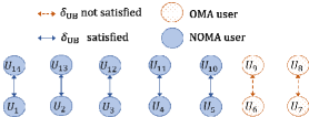
IV-A Figure 2 : Adaptive user pairing.
In [NearFar1 , NearFar2 , GenPairing ] , the authors have shown that pairing of near users with far users achieves better data rates. Motivated by this, we initially sort the users based on their s and group the near users with far users. For each user, we then define the rate achievable with as the minimum required rate (i.e., R i ¯ = RiOMA ¯ subscript 𝑅 𝑖 RiOMA \overline{R_{i}}~{}=~{}\lx@glossaries@gls@link{main}{RateO}{\leavevmode R_{i}^{\text{\tiny OMA}}} 19 δ 𝛿 \delta δ UB subscript δ UB \lx@glossaries@gls@link{main}{delta}{\leavevmode\delta}_{\text{\tiny UB}} 19 2 γ1CSI ≥ … ≥ γ 14 CSI γ1CSI … superscript subscript 𝛾 14 CSI \lx@glossaries@gls@link{main}{Gamma1CSI}{\leavevmode\gamma_{1}^{\text{\tiny CSI}}}\geq...\geq\gamma_{14}^{\text{\tiny CSI}}
IV-B
In this section, we present maximum achieving power allocation procedure for the