A quantum Monte Carlo method on asymptotic Lefschetz thimbles for quantum spin systems:
An application to the Kitaev model in a magnetic field

Abstract

The quantum Monte Carlo method on asymptotic Lefschetz thimbles is a numerical algorithm devised specifically for alleviation of the sign problem appearing in the simulations of quantum many-body systems. In this method, the sign problem is alleviated by shifting the integration domain for the auxiliary fields, appearing for example in the conventional determinant quantum Monte Carlo method, from real space to an appropriate manifold in complex space. Here we extend this method to quantum spin models with generic two-spin interactions, by using the Hubbard-Stratonovich transformation to decouple the exchange interactions and the Popov-Fedotov transformation to map the quantum spins to complex fermions. As a demonstration, we apply the method to the Kitaev model in a magnetic field whose ground state is predicted to deliver a topological quantum spin liquid with non-Abelian anyonic excitations. To illustrate how the sign problem is alleviated in this method, we visualize the asymptotic Lefschetz thimbles in complex space, together with the saddle points and the zeros of the fermion determinant. We benchmark our method in the low-temperature region in a magnetic field and show that the sign of the action is recovered considerably and unbiased numerical results are obtained with sufficient precision.

I Introduction

The quantum Monte Carlo (QMC) simulation based on the path integral formalism is one of the most widely used methods to study quantum many-body problems. In this method, the action of the system in $d$ dimensions is written by a functional integral in terms of the auxiliary fields in $(d+1)$ dimensions, and the integration is performed by means of the importance sampling on the configurations of the auxiliary fields with the use of the action as the Monte Carlo (MC) weight for each configuration. The QMC method is a versatile tool as it provides numerically exact results within the statistical errors in principle, but it often encounters with a serious obstacle called the sign problem. It originates from the fact that, except in a few limited cases, the action is complex, rather than positive definite real, which makes hard to use it as the MC weight. In the conventional QMC method, the complex action has been dealt with by using the reweighting technique. In this technique, the MC sampling is done by the real part of the action $\mathrm{Re}\mathcal{S}(\bm{\varphi})$, where $\bm{\varphi}$ represents the auxiliary fields, and the imaginary part $\mathrm{Im}\mathcal{S}(\bm{\varphi})$ is measured together with the observable $O(\bm{\varphi})$; namely, the thermal average of $O(\bm{\varphi})$ is computed as

$$\braket{O}=\frac{\int d\bm{\varphi}O(\bm{\varphi})e^{-\mathcal{S}(\bm{\varphi})}}{\int d\bm{\varphi}e^{-\mathcal{S}(\bm{\varphi})}}=\frac{\big{\langle}O(\bm{\varphi})e^{-i\mathrm{Im}\mathcal{S}(\bm{\varphi})}\big{\rangle}_{\mathrm{Re}\mathcal{S}(\bm{\varphi})}}{\big{\langle}e^{-i\mathrm{Im}\mathcal{S}(\bm{\varphi})}\big{\rangle}_{\mathrm{Re}\mathcal{S}(\bm{\varphi})}},$$ (1)

where $\langle A\rangle_{\mathrm{Re}\mathcal{S}(\bm{\varphi})}$ denotes the thermal average of $A$ obtained with the weight of $e^{-\mathrm{Re}\mathcal{S}(\bm{\varphi})}$. This reweighting is used in a broad range of the research fields; for instance, it has been used in the so-called determinant QMC (D-QMC) method for many fermionic models in solid state physics Blankenbecler et al. (1981); Scalapino and Sugar (1981); von der Linden (1992); Loh and Gubernatis (1992); dos Santos (2003); Bercx et al. (2003); Assaad and Evertz (2008); Sato and Assaad (2021). The problem is that the practical evaluation of Eq. (1) is exponentially difficult as follows. By definition, the evaluation is feasible when the ensemble sampled according to $\mathrm{Re}\mathcal{S}(\bm{\varphi})$ has a sufficient overlap with that by the full action $\mathcal{S}(\bm{\varphi})$. Consequently, the method is successful only as long as the average sign, which is defined by

$$S_{\mathrm{D\textnormal{-}QMC}}=\left\lvert\big{\langle}e^{-i\mathrm{Im}\mathcal{S}(\bm{\varphi})}\big{\rangle}_{\mathrm{Re}\mathcal{S}(\bm{\varphi})}\right\lvert,$$ (2)

retains a sufficiently large value. In general, however, $S_{\mathrm{D\textnormal{-}QMC}}$ becomes exponentially small with respect to the inverse temperature and the system size. Thus, simulations using the reweighting method become exponentially harder at lower temperatures and for larger system sizes. This is the notorious sign problem, which has hampered full understanding of many interesting quantum many-body phenomena, such as exotic phases in quantum chromodynamics Philipsen (2009); Aarts (2016), physics of Feshbach resonances in cold atomic Fermi gases Inguscio et al. (2007); Bloch et al. (2008); Giorgini et al. (2008), possible superconductivity in doped Mott insulators Baeriswyl et al. (1995); Lee et al. (2006), and quantum spin liquids in frustrated quantum spin systems Wen (2007); Balents (2010); Lacroix et al. (2011); Diep (2013); Savary and Balents (2017). We note that the sign problem is shown to be an NP-hard problem for Ising spin-glass systems Troyer and Wiese (2005), which suggests that its fundamental solution is unlikely to be available.

Under this circumstance, however, there have been a lot of efforts to avoid or alleviate the sign problem. One of such efforts is to extend the auxiliary fields from real to complex and shift the integration domain form real space to an appropriate manifold in complex space. An approach based on this scheme is employing the idea of the Lefschetz thimbles Witten (2010a, b). This method also demonstrated its power in a variety of applications in the field of high-energy physics Cristoforetti et al. (2012, 2013); Fujii et al. (2013); Mukherjee et al. (2013); Cristoforetti et al. (2014a, b); Aarts et al. (2014); Tanizaki (2015); Renzo and Eruzzi (2015); Fujii et al. (2015a); Kanazawa and Tanizaki (2015); Fukushima and Tanizaki (2015); Fujii et al. (2015b); Tanizaki et al. (2016); Tsutsui and Doi (2016); Alexandru et al. (2016a, b, 2017a, 2017b); Tanizaki et al. (2017); Alexandru et al. (2017c); M. Fukuma (2017); Renzo and Eruzzi (2018); Bluecher et al. (2018); Alexandru et al. (2018a, b, c) and solid state physics Mukherjee and Cristoforetti (2014); Ulybyshev and Valgushev (2017); Ulybyshev et al. (2019); Fukuma et al. (2019a, b); Ulybyshev et al. (2020a, b); Wynen et al. (2021). It is, however, important to note that in the case of fermionic systems, straightforward application of the Lefschetz thimble method faces difficulties in practice; while the efficient calculations require prior knowledge of the structure of the Lefschetz thimbles in complex space, it is in general unknown a priori Alexandru et al. (2016a). To overcome the difficulty, the possibility of integrating on an asymptotic form of the Lefscehtz thimbles was proposed, which in principle enables one to take into account all the relevant thimbles without prior knowledge of their structure Alexandru et al. (2016b). One of the most important improvements along this approach is a technique similar to the parallel tempering which was demonstrated to give unbiased results with great efficiency Alexandru et al. (2017c); M. Fukuma (2017); Fukuma et al. (2019a, b). Despite all these achievements, however, to the best of our knowledge, the previous studies were all limited to the models with interacting mobile fermions like the Hubbard model, and there are no applications to quantum spin models where the fermions are immobile and only their spin degrees of freedom remain active.

In this paper, we develop the QMC method based on the asymptotic Lefscehtz thimbles, which we call the ALT-QMC method, into a form applicable to quantum spin models with generic two-spin interactions. In our framework, we obtain the functional integral of the action by two steps. The first step is the Hubbard-Stratonovich transformation Stratonovich (1958); Hubbard (1959) in which the exchange interactions are decoupled into one-body terms by introducing the auxiliary fields. The second step is the Popov-Fedotov transformation Popov and Fedotov (1988); *popov_psim_184_1991 by which the quantum spins are mapped to complex fermions. These end up with the functional integral for the generic quantum spin Hamiltonian to which the ALT-QMC method can be applied. We demonstrate the efficiency of the method for the Kitaev model in a magnetic field, which has recently attracted much attention since it delivers a topological quantum spin liquid with non-Abelian anyonic excitations. We visualize the asymptotic Lefschetz thimbles in complex space, together with the saddle points and the zeros of the fermion determinant. By careful comparison with the results obtained by the D-QMC method, we show that our ALT-QMC method indeed alleviates the sign problem and potentially extends the accessible parameter regions to lower temperatures and larger system sizes.

The paper is structured as follows. In Sec. II, we briefly review the Lefschetz thimble method. We introduce the general formalism of the Lefschetz thimbles in Sec. II.1 and the asymptotic Lefschetz thimbles in Sec. II.2. In Sec. III, we construct the framework for the ALT-QMC method applicable to generic spin models. After introducing a class of the models to which the method can be applied in Sec. III.1, we introduce the Hubbard-Stratonovich transformation in Sec. III.2, the Popov-Fedotov transformation in Sec. III.3, and derive the functional integral of the action in Sec. III.4. In Sec. III.5, we make some remarks on the implementation of the simulation and the definitions of the metrics to estimate the severity of the sign problem. In Sec. IV, we present the results by the ALT-QMC method for the Kitaev model in a magnetic field. After introducing the model in Sec. IV.1, we visualize the structure of the Lefschetz thimbles in complex space and present the benchmark of the ALT-QMC technique for a small system in Secs. IV.2 and IV.3, respectively. In Sec. IV.4, we show the results for the Kitaev model in a magnetic field for a larger system size. Finally, Sec. V is devoted to the summary and outlook.

II Lefschetz thimble method

In this section, we briefly review the Lefschetz thimble method. In Sec. II.1, we describe the fundamentals of the Lefschetz thimbles, and in Sec. II.2, we present the framework of asymptotic Lefschetz thimbles.

II.1 Lefschetz thimbles

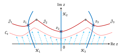
Figure 1: Schematic illustration of the Lefschetz thimbles and the asymptotic ones for a single auxiliary field $z$. The solid red lines represent the true Lefschetz thimbles $\mathcal{J}_{\nu}$ associated with the saddle points $z_{\nu}$ (dark blue crosses) and the zeros of the fermion determinant separating different thimbles (gray dots). The solid blue lines represent the antithimbles $\mathcal{K}_{\nu}$. The dotted red line represents the asymptotic Lefschetz thimble $\mathcal{C}_{t}$ obtained by the time evolution from the real axis which is represented by the dashed blue arrows.

In general, one can estimate the action $\mathcal{S}(\bm{\varphi})$ by extending the functional integral to complex space by analytic continuation from the real auxiliary fields $\bm{\varphi}$ to the complex ones $\bm{z}$. In fact, one can define an integration path in the complex space along which the following two properties are satisfied: (i) Along the integration path, the real part of the action, $\mathrm{Re}\mathcal{S}(\bm{z})$, decreases the fastest when moving towards the saddle point, and (ii) the imaginary part of the action, $\mathrm{Im}\mathcal{S}(\bm{z})$, is constant on the integration path which takes the same value at the saddle point. Such a path is called the Lefschetz thimble Witten (2010a, b). In general, the action $\mathcal{S}(\bm{z})$ may have multiple saddle points $\bm{z}_{\nu}$ with multiple Lefschetz thimbles $\mathcal{J}_{\nu}$ associated to them (hereafter we use $\nu$ for labeling the saddle points and associated Lefschetz thimbles), and therefore, the original integral in the real space is equivalent to the sum of the integrals over the Lefschetz thimbles in the complex space. It is important to note that in fermionic systems, different Lefschetz thimbles are separated from each other by the points where the fermion determinant vanishes and the effective action diverges. See the schematic in Fig. 1.

One can identify the saddle points $\bm{z}_{\nu}$ of the action $\mathcal{S}(\bm{z})$ by solving the set of equations

$$\frac{\partial\mathcal{S}(\bm{z})}{\partial z_{l}}\bigg{|}_{\bm{z}=\bm{z}_{\nu}}=0,$$ (3)

and the Lefschetz thimble $\mathcal{J}_{\nu}$ attached to the saddle point $\bm{z}_{\nu}$ by the flow equation

$$\frac{dz_{l}}{dt}=-\left[\frac{\partial\mathcal{S}(\bm{z})}{\partial z_{l}}\right]^{*},$$ (4)

where $l$ is the index of the auxiliary variable $\bm{z}$, and $dz_{l}/dt$ means the “time” derivative of the auxiliary variable $z_{l}$. Indeed the Lefschetz thimbles determined by Eq. (4) satisfy the two properties described above.

Besides the thimbles $\mathcal{J}_{\nu}$, the so-called antithimbles $\mathcal{K}_{\nu}$ attached to the saddle point $\bm{z}_{\nu}$ are also important in the following calculations. The antithimble for the saddle point $\bm{z}_{\nu}$ is defined by

$$\frac{dz_{l}}{dt}=+\left[\frac{\partial\mathcal{S}(\bm{z})}{\partial z_{l}}\right]^{*}.$$ (5)

Once all the thimbles $\mathcal{J}_{\nu}$ and the antithimbles $\mathcal{K}_{\nu}$ are identified, one can calculate the statistical average of an observable $O(\bm{z})$ by using the sum of the integrals over $\mathcal{J}_{\nu}$ Witten (2010a, b):

$$\braket{O}=\frac{\sum_{\nu}n_{\nu}e^{-i\mathrm{Im}\mathcal{S}(\bm{z}_{\nu})}\int_{\mathcal{J}_{\nu}}d\bm{z}O(\bm{z})e^{-\mathrm{Re}\mathcal{S}(\bm{z})}}{\sum_{\nu}n_{\nu}e^{-i\mathrm{Im}\mathcal{S}(\bm{z}_{\nu})}\int_{\mathcal{J}_{\nu}}d\bm{z}e^{-\mathrm{Re}\mathcal{S}(\bm{z})}},$$ (6)

where $n_{\nu}$ is an integer given by the number of the intersections between the corresponding antithimble $\mathcal{K}_{\nu}$ and the original integration domain in the real space. Thus, one can in principle compute the original integral in the real space by the integrals on the Lefschetz thimbles in the complex space. The important point here is that the sign problem is alleviated since $\mathrm{Im}\mathcal{S}(\bm{z}_{\nu})$ is constant on each Lefschetz thimble and put outside the integrals in Eq. (6).

II.2 Asymptotic Lefschetz thimbles

Although the framework of the Lefschetz thimbles is exact and suppresses the sign problem, the practical application is not straightforward as it is difficult to identify all the thimbles $\mathcal{J}_{\nu}$ with all the corresponding coefficients $n_{\nu}$. For this reason, the Lefschetz thimble technique has been applied only to some limited cases. For instance, the method was applied when the models are sufficiently simple and all the Lefschetz thimbles can be identified, for the bosonic Aarts et al. (2014); Tanizaki (2015); Fukushima and Tanizaki (2015) and fermionic cases Kanazawa and Tanizaki (2015); Tanizaki et al. (2016). Also, QMC simulations were performed on dominant thimbles for both bosonic Renzo and Eruzzi (2015); Tsutsui and Doi (2016); Cristoforetti et al. (2013); Fujii et al. (2013); Mukherjee et al. (2013); Cristoforetti et al. (2014a, b) and fermionic systems Fujii et al. (2015a, b); Alexandru et al. (2016a). However, especially in the fermionic systems, the integration over the dominant thimbles is often insufficient to obtain the precise estimate of the observables; it is not obvious how to take into account all the relevant contributions.

To overcome the difficulty, an alternative method was proposed Alexandru et al. (2016b), in which the integral is taken on an asymptotic form of the Lefschetz thimbles rather than the true Lefschetz thimbles. This technique enables one to take into account the contributions from all the relevant thimbles without knowing all the true thimbles a priori Alexandru et al. (2016b). It is achieved by starting the process of finding the thimbles not from the saddle points $\bm{z}_{\nu}$ by solving Eqs. (3) and (4) but rather from the original integration domain with time evolution by using Eq. (5). Such time evolution gradually deforms the integration domain to a manifold in the complex space, as schematically shown in Fig. 1. The manifold approaches the true Lefschetz thimbles asymptotically, and hence the time evolved manifold is called the asymptotic Lefschetz thimbles, which we denote as $\mathcal{C}_{t}$ at time $t$. In this time evolution, some special points will flow to the saddle points $\bm{z}_{\nu}$ and other points close to them will flow closely to $\mathcal{J}_{\nu}$ attached to $\bm{z}_{\nu}$. All the points except the ones flowing to the saddle points will eventually flow to the singularities of the action in the long time limit, which are zeros of the fermion determinant in the fermionic problems. As such, the flow from the real space can collect the contributions from all the relevant thimbles once the sampling and the time evolution are performed appropriately.

Using the above method, one can perform MC sampling on the asymptotic Lefschetz thimbles $\mathcal{C}_{t}$ obtained by time evolution of the samples proposed in the real space. The regions with large MC weights in the real space become even larger in the complex space because the time evolution according to Eq. (5) always increases the real part of the action. On the other hand, the imaginary part of the action on $\mathcal{C}_{t}$ remains as the original one in the real space because the time evolution keeps the imaginary part of the action unchanged. Thus, in the regions of $\mathcal{C}_{t}$ with large MC weights, the fluctuation of the phase $e^{-i\mathrm{Im}\mathcal{S}(\bm{z})}$ tends to be suppressed, and hence, the sign problem is alleviated for the samples on the complex manifold $\mathcal{C}_{t}$ compared to the original ones in the real space.

Mathematically, the deformation from the real space to the complex manifold $\mathcal{C}_{t}$ by Eq. (5) corresponds to a change of variables from real $\bm{\varphi}$ to complex $\bm{z}$ as

$$\braket{O}=~{} \frac{\int_{\mathcal{C}_{t}}d\bm{z}O(\bm{z})e^{-\mathcal{S}(\bm{z})}}{\int_{\mathcal{C}_{t}}d\bm{z}e^{-\mathcal{S}(\bm{z})}}$$

$$=~{} \frac{\int d\bm{\varphi}O\bm{(}\bm{z}(\bm{\varphi})\bm{)}e^{-\mathcal{S}\bm{(}\bm{z}(\bm{\varphi})\bm{)}}\mathrm{det}J}{\int d\bm{\varphi}e^{-\mathcal{S}\bm{(}\bm{z}(\bm{\varphi})\bm{)}}\mathrm{det}J},$$ (7)

where $J$ is the Jacobian given by $J_{l,m}=\partial z_{l}/\partial\varphi_{m}$; the integrals in the first line are taken on the asymptotic Leschetz thimbls $\mathcal{C}_{t}$ in the complex space, while those in the second line are taken on the original domain in the real space. Equation (7) indicates that $\bm{\varphi}$ parametrize the asymptotic Lefschetz thimbles $\mathcal{C}_{t}$ in the complex space after a flow time $t$. This allows one to estimate the statistical average by proposing $\bm{\varphi}$ in the real space by the Markov chain MC sampling and evolving them to the asymptotic Lefschetz thimbles $\mathcal{C}_{t}$ by Eq. (5). During the time evolution, the Jacobian along the flows of the samples can be calculated by

$$\frac{dJ_{l,m}}{dt}=\left[\sum_{n}\frac{\partial^{2}\mathcal{S}\left(\bm{z}\right)}{\partial z_{l}\partial z_{n}}J_{n,m}\right]^{*},$$ (8)

with the initial condition $J=\mathbb{I}$ (identity matrix).

This technique allows one to perform MC sampling without prior knowledge of relevant Lefschetz thimbles $\mathcal{J}_{\nu}$ and the corresponding saddle points $\bm{z}_{\nu}$. In the simulation, the MC sampling is performed for the configurations of the real auxiliary variables $\bm{\varphi}$ by using $e^{-\mathrm{Re}\mathcal{S}\bm{(}\bm{z}(\bm{\varphi})\bm{)}}$ as the MC weight, and the integral in Eq. (7) is computed after the time evolution by measuring the phase $e^{-i\mathrm{Im}\mathcal{S}\bm{(}\bm{z}(\bm{\varphi})\bm{)}}$ and $\mathrm{det}J$ together with the observable $O\bm{(}\bm{z}(\bm{\varphi})\bm{)}$ as

$$\braket{O}=\frac{\big{\langle}O\bm{(}\bm{z}(\bm{\varphi})\bm{)}e^{-i\mathrm{Im}\mathcal{S}\bm{(}\bm{z}(\bm{\varphi})\bm{)}}\mathrm{det}J\big{\rangle}_{\mathrm{Re}\mathcal{S}\bm{(}\bm{z}(\bm{\varphi})\bm{)}}}{\big{\langle}e^{-i\mathrm{Im}\mathcal{S}\bm{(}\bm{z}(\bm{\varphi})\bm{)}}\mathrm{det}J\big{\rangle}_{\mathrm{Re}\mathcal{S}\bm{(}\bm{z}(\bm{\varphi})\bm{)}}}.$$ (9)

Here, in order to save the computational time during the calculation of Eq. (9), the determinant of the Jacobian, $\mathrm{det}J$, is included into the observable $O\bm{(}\bm{z}(\bm{\varphi})\bm{)}$ and is calculated only once per MC sweep, following the previous studies Ulybyshev et al. (2019, 2020a, 2020b).

Let us remark on the dimension of the original integration domain, the true and asymptotic Lefschetz thimbles, and the zeros of the fermion determinant. The dimension of the original integration domain in the real space is defined by the number of the auxiliary fields $\bm{\varphi}$, $N_{\bm{\varphi}}$. The domain $\mathbb{R}^{N_{\bm{\varphi}}}$ is evolved by Eq. (5) into a manifold $\mathbb{R}^{N_{\bm{\varphi}}}$ embedded in the complex domain $\mathbb{C}^{N_{\bm{\varphi}}}$. Therefore, the asymptotic Lefschetz thimbles are $\mathbb{R}^{N_{\bm{\varphi}}}$-dimensional manifolds. The true Lefschetz thimbles are also $\mathbb{R}^{N_{\bm{\varphi}}}$-dimensional manifolds. On the other hand, the zeros of the fermion determinant constitute $\mathbb{C}^{N_{\bm{\varphi}}-1}$-dimensional manifolds embedded in $\mathbb{C}^{N_{\bm{\varphi}}}$ in the generic case Alexandru et al. (2016b).

III Quantum Monte Carlo method for generic quantum spin models

In this section, we show a QMC method based on the asymptotic Lefschetz thimbles, which we call the ALT-QMC method, applicable to a generic quantum spin model with arbitrary two-spin interactions and the Zeeman coupling. While this technique can be applied to generic spin magnitudes $S$, for the sake of simplicity, we limit our description to the $S=1/2$ case. In Sec. III.1, we introduce the generic model to which the ALT-QMC method can be applied. In Sec. III.2, we introduce the Hubbard-Stratonovich transformation to decouple the two-spin interactions. In Sec. III.3, we describe an exact mapping from the quantum spins to complex fermions by means of the Popov-Fedotov transformation. In Sec. III.4, we discretize the partition function via the Suzuki-Trotter decomposition and derive the functional integral of the action. In Sec. III.5, we make a remark on the details of the implementation and the estimate of the sign problem.

III.1 Model

We consider a generic $S=1/2$ model with arbitrary two-spin interactions, whose Hamiltonian is given by

$$\mathcal{H}=-\sum_{p,q}\sum_{\alpha,\beta}K_{p,q}^{\alpha,\beta}\sigma_{p}^{\alpha}\sigma_{q}^{\beta}-\sum_{p}\sum_{\alpha}h_{p}^{\alpha}\sigma_{p}^{\alpha},$$ (10)

where the spin degree of freedom at site $p$ is described by the Pauli matrices $\sigma_{p}^{\alpha}$, and $K_{p,q}^{\alpha,\beta}$ is the coupling constant for the two-spin interaction ($\alpha$, $\beta=x$, $y$, $z$); the second term describes the Zeeman coupling to a magnetic field whose $\alpha$ component at site $p$ is denoted as $h_{p}^{\alpha}$. Both $K_{p,q}^{\alpha,\beta}$ and $h_{p}^{\alpha}$ can be spatially inhomogeneous. The following formulation is applicable to the model in Eq. (10) on any lattice geometry with any boundary conditions.

III.2 Hubbard-Stratonovich transformation

For constructing the QMC method based on the path integral formalism, we decompose the two-body interactions by using the Hubbard-Stratonovich transformation Stratonovich (1958); Hubbard (1959). Among several choices, we use the transformation with continuous auxiliary variables which is suitable for the present purpose to develop the ALT-QMC method. Specifically, rewriting the interaction term in Eq. (10) as

$$-K_{p,q}^{\alpha,\beta}\sigma_{p}^{\alpha}\sigma_{q}^{\beta}=-\frac{1}{2}K_{p,q}^{\alpha,\beta}\left[\left(\sigma_{p}^{\alpha}+\sigma_{q}^{\beta}\right)^{2}-2\right],$$ (11)

we decompose it by using the Hubbard-Stratonovich transformation as

$$\mathrm{exp}\left[\frac{\Delta}{2}K_{p,q}^{\alpha,\beta}\left(\sigma_{p}^{\alpha}+\sigma_{q}^{\beta}\right)^{2}\right]=\sqrt{\frac{\Delta}{2\pi}}\int d\varphi_{p,q}^{\alpha,\beta}$$

$$\times\mathrm{exp}\left[-\frac{\Delta}{2}\left(\varphi_{p,q}^{\alpha,\beta}\right)^{2}-\Delta\varphi_{p,q}^{\alpha,\beta}\sqrt{K_{p,q}^{\alpha,\beta}}\left(\sigma_{p}^{\alpha}+\sigma_{q}^{\beta}\right)\right],$$ (12)

where $\Delta$ is a positive constant that will be introduced in the Suzuki-Trotter decomposition in Sec. III.4. Note that the sign of $K_{p,q}^{\alpha,\beta}$ can be both positive and negative; in case of $K_{p,q}^{\alpha,\beta}<0$, $\sqrt{K_{p,q}^{\alpha,\beta}}$ in Eq. (12) becomes a pure imaginary. Note that, in this formulation, we introduce one continuous real auxiliary variable of Gaussian type, $\varphi_{p,q}^{\alpha,\beta}$, for each interaction term $-K_{p,q}^{\alpha,\beta}\sigma_{p}^{\alpha}\sigma_{q}^{\beta}$, which will save the computational cost; see Sec. III.5.

III.3 Popov-Fedotov transformation

To utilize the framework based on the asymptotic Lefschetz thimble technique for the fermionic systems, we proceed with mapping from the quantum spins to complex fermions via the Popov-Fedotov transformation Popov and Fedotov (1988); *popov_psim_184_1991. To begin with, let us express the spin degree of freedom described in terms of the Pauli matrices by complex fermions by using

$$\sigma_{p}^{\alpha}\rightarrow\sum_{\gamma,\gamma^{\prime}}f_{p,\gamma}^{\dagger}\sigma_{\gamma,\gamma^{\prime}}^{\alpha}f_{p,\gamma^{\prime}},$$ (13)

where $f_{p,\gamma}^{\dagger}$ and $f_{p,\gamma}$ are the creation and annihilation operators of a complex fermion, respectively, at site $p$ with spin $\gamma=\uparrow$ or $\downarrow$. It is important to note that the relation in Eq. (13) enlarges the size of the Hilbert space per site from two for the original spin to four for the fermion as $f_{p,\uparrow}^{\dagger}\ket{0}$, $f_{p,\downarrow}^{\dagger}\ket{0}$, $\ket{0}$, $f_{p,\uparrow}^{\dagger}f_{p,\downarrow}^{\dagger}\ket{0}$ ($\ket{0}$ is the vacuum). The first two states with fermion occupation number unity are physical, whereas the last two are unphysical. One can eliminate the unphysical states by adding a term to the fermion Hamiltonian, which gives zero when acting on the physical Hilbert space and keeps the partition function intact. The explicit form of such a term is given by Popov and Fedotov (1988); *popov_psim_184_1991

$$\mathcal{H}_{\mu}=\frac{i\pi}{2\beta}\sum_{p}\left(\sum_{\gamma}f_{p,\gamma}^{\dagger}f_{p,\gamma}-1\right),$$ (14)

which corresponds to the introduction of an imaginary chemical potential $-i\pi/2\beta$ depending on the inverse temperature $\beta=1/T$ (we set the Boltzmann constant $k_{\rm B}=1$). It is straightforward to verify that the trace over the unphysical states vanishes for the total Hamiltonian including Eq. (14) because the contributions from $\ket{0}$ and $f_{p,\uparrow}^{\dagger}f_{p,\downarrow}^{\dagger}\ket{0}$ eliminate each other. Hence, the following relation for the partition function holds exactly:

$$\mathcal{Z}=\mathrm{Tr}\left[\mathrm{exp}\left(-\beta\mathcal{H}\right)\right]=\mathrm{Tr}\left\{\mathrm{exp}\left[-\beta\left(\mathcal{H}_{f}+\mathcal{H}_{\mu}\right)\right]\right\},$$ (15)

where $\mathcal{H}_{f}$ is the fermion Hamiltonian obtained from Eq. (10) via the transformation in Eq. (13).

This method provides an exact mapping from quantum spins to complex fermions without introducing any unphysical states. It is applicable to any $S=1/2$ models with any two-spin interactions. Furthermore, since the mapping is defined by the local (onsite) transformation in Eq. (13), it can be applied to any lattice geometry with any boundary conditions. Further details and applications of this method are found, for example, in Refs. Popov and Fedotov (1988); Gros and Johnson (1990); Stein and Oppermann (1991); Veits et al. (1994); Bouis and Kiselev (1999); Azakov et al. (2000); Kiselev and Oppermann (2000a, b); Kiselev et al. (2001, 2002, 2003); Coleman and Mao (2004); Dillenschneider and Richert (2006); Prokof’ev and Svistunov (2011).

III.4 Path integral of the action

By combining the two transformations above, we obtain the expression of the action to which the ALT-QMC method is applicable. First, let us decompose the entire fermionized Hamiltonian into the two-body parts and the one-body part as

$$\mathcal{H}_{f}+\mathcal{H}_{\mu}=\sum_{m=1}^{N_{I}-1}\mathcal{H}_{m}+\left(\mathcal{H}_{h}+\mathcal{H}_{\mu}\right)=\sum_{m=1}^{N_{I}}\mathcal{H}_{m},$$ (16)

where $\mathcal{H}_{m}$ for $1\leq m\leq N_{I}-1$ is the Hamiltonian obtained by fermionizing $-\sum_{p,q}K_{p,q}^{\alpha,\beta}\sigma_{p}^{\alpha}\sigma_{q}^{\beta}$ with a particular set of $\alpha$ and $\beta$, and $\mathcal{H}_{h}$ stands for the Zeeman coupling term in Eq. (10); $\mathcal{H}_{N_{I}}$ denotes the one-body part, $\mathcal{H}_{h}+\mathcal{H}_{\mu}$. With this form, we introduce the Suzuki-Trotter decomposition for the operator $\mathrm{exp}[-\beta(\mathcal{H}_{f}+\mathcal{H}_{\mu})]$ in Eq. (15) as

$$\mathrm{exp}\left[-\beta\left(\mathcal{H}_{f}+\mathcal{H}_{\mu}\right)\right]\approx\left[\prod_{m=1}^{N_{I}}\mathrm{exp}\left(-\Delta\mathcal{H}_{m}\right)\right]^{N_{\beta}},$$ (17)

where $N_{\beta}$ is the number of the Suzuki-Trotter discretization in the imaginary-time direction; $\Delta=\beta/N_{\beta}$. Note that the approximation in Eq. (17) is valid up to $\mathcal{O}(\Delta^{2})$. Then, the partition function in Eq. (15) is expressed as

$$\mathcal{Z}\approx\mathrm{Tr}\left\{\left[\prod_{m=1}^{N_{I}}\mathrm{exp}\left(-\Delta\mathcal{H}_{m}\right)\right]^{N_{\beta}}\right\}.$$ (18)

The exact partition function will be obtained in the limit of $\Delta\rightarrow 0$ and $N_{\beta}\to\infty$. Note that the systematic error in the discretized partition function $\mathcal{Z}$ is again of $\mathcal{O}(\Delta^{2})$ owing to the property of the trace operation Sandvik (2010).

The partition function $\mathcal{Z}$ in Eq. (18), with the constant contribution in Eq. (14) placed outside the integral, can be expressed by using anticommuting Grassmann variables $\psi_{p,\gamma}$ and $\bar{\psi}_{p,\gamma}$ as

$$\mathcal{Z}=e^{\frac{i\pi N_{S}}{2}}\int \prod_{p,\gamma}d\bar{\psi}_{p,\gamma}d\psi_{p,\gamma}\mathrm{exp}\left(-\sum_{p,\gamma}\bar{\psi}_{p,\gamma}\psi_{p,\gamma}\right)$$

$$\times\braket{-\bar{\psi}}{\left[\prod_{m=1}^{N_{I}}\mathrm{exp}\left(-\Delta\mathcal{H}_{m}\right)\right]^{N_{\beta}}}{\psi},$$ (19)

where $\ket{\psi}=\mathrm{exp}(-\sum_{p,\gamma}\psi_{p,\gamma}f_{p,\gamma}^{\dagger})\ket{0}$ and $\bra{\bar{\psi}}=\bra{0}\mathrm{exp}(-\sum_{p,\gamma}f_{p,\gamma}\bar{\psi}_{p,\gamma})$ are the fermionic coherent states, and $N_{S}$ is the system size; here, $\mathcal{H}_{N_{I}}$ does not include the complex constant $-i\pi N_{S}/2\beta$. Then, by inserting the identity relation for the fermionic coherent states we obtain

$$\mathcal{Z}=e^{\frac{i\pi N_{S}}{2}}\int \prod_{l=1}^{N_{\beta}}\prod_{m=1}^{N_{I}}\prod_{p,\gamma}d\bar{\psi}_{p,\gamma}^{l,m}d\psi_{p,\gamma}^{l,m}$$

$$\mathrm{exp}\left(-\sum_{l=1}^{N_{\beta}}\sum_{m=1}^{N_{I}}\sum_{p,\gamma}\bar{\psi}_{p,\gamma}^{l,m+1}\psi_{p,\gamma}^{l,m}\right)$$

$$\times\prod_{l=1}^{N_{\beta}}\prod_{m=1}^{N_{I}}\braket{\bar{\psi}^{l,m}}{\mathrm{exp}\left(-\Delta\mathcal{H}_{l,m}\right)}{\psi^{l,m}}.$$ (20)

where $l$ is the label for the Suzuki-Trotter slice, each containing in total $N_{I}$ slices numbered by $m$, and for all of the slices, the aniticommuting Grassmann variables $\psi_{p,\gamma}^{l,m}$ and $\bar{\psi}_{p,\gamma}^{l,m}$ are defined. Here, the Grassmann variables satisfy the boundary conditions:

$$-\bar{\psi}_{p,\gamma}=\bar{\psi}_{p,\gamma}^{1,1}=\bar{\psi}_{p,\gamma}^{N_{\beta},N_{I}+1},$$

$$\psi_{p,\gamma}^{N_{\beta},N_{I}}=\psi_{p,\gamma},\quad\bar{\psi}_{p,\gamma}^{l,N_{I}+1}=\bar{\psi}_{p,\gamma}^{l+1,1}.$$ (21)

Next, with the help of the Hubbard-Stratonovich transformation in Eq. (12), we obtain the following relation for each matrix element in Eq. (20) with the two-body terms:

$$\mathrm{exp}\left(-\Delta\mathcal{H}_{l,m}\right)$$

$$=\mathrm{exp}\left[\frac{\Delta}{2}\sum_{n}K_{n}^{m}\left(\mathcal{P}_{n}^{m}\right)^{2}-\Delta\sum_{n}K_{n}^{m}\right]$$

$$=\left(\frac{\Delta}{2\pi}\right)^{\frac{N_{m}}{2}}\mathrm{exp}\left(-\Delta\sum_{n}K_{n}^{m}\right)\int\prod_{n}d\varphi_{n}^{m}$$

$$\qquad\mathrm{exp}\left[-\frac{\Delta}{2}\sum_{n}\left(\varphi_{n}^{m}\right)^{2}-\Delta\sum_{n}\varphi_{n}^{m}\sqrt{K_{n}^{m}}\mathcal{P}_{n}^{m}\right],$$ (22)

where $n$ denotes a pair of $p$ and $q$ for the two-body terms ($1\leq m\leq N_{I}-1$), $N_{m}$ stands for the total number of interaction terms in a particular $\mathcal{H}_{l,m}$, and $\mathcal{P}_{n}^{m}$ is the bilinear fermionic operator obtained by replacing quantum spins in Eq. (12) with the complex fermions as in Eq. (13):

$$\mathcal{P}_{n}^{m}=\sum_{\gamma,\gamma^{\prime}}(f_{p,\gamma}^{\dagger}\sigma_{\gamma,\gamma^{\prime}}^{\alpha}f_{p,\gamma^{\prime}}+f_{q,\gamma}^{\dagger}\sigma_{\gamma,\gamma^{\prime}}^{\beta}f_{q,\gamma^{\prime}}).$$ (23)

By using the relation for the Grassmann variables for a matrix $M$ Ulybyshev et al. (2013); Smith and von Smekal (2014); Buividovich and Polikarpov (2012)

$$\braket{\bar{\psi}^{l,m}}{\mathrm{exp}\left(\sum_{k,k^{\prime}}f_{k}^{\dagger}M_{k,k^{\prime}}f_{k^{\prime}}\right)}{\psi^{l,m}}$$

$$=\mathrm{exp}\left[\sum_{k,k^{\prime}}\bar{\psi}_{k}^{l,m}\mathrm{exp}\left(M\right)_{k,k^{\prime}}\psi_{k^{\prime}}^{l,m}\right],$$ (24)

where $k=\{p,\gamma\}$ and $k^{\prime}=\{q,\gamma^{\prime}\}$, one can write each interaction term in Eq. (20) as

$$\braket{\bar{\psi}^{l,m}}{\mathrm{exp}\left(-\Delta\mathcal{H}_{l,m}\right)}{\psi^{l,m}}$$

$$=\left(\frac{\Delta}{2\pi}\right)^{\frac{N_{m}}{2}}\mathrm{exp}\left(-\Delta\sum_{n}K_{n}^{m}\right)\int\prod_{n}d\varphi_{n}^{m}$$

$$\mathrm{exp}\left[-\frac{\Delta}{2}\sum_{n}\left(\varphi_{n}^{m}\right)^{2}+\sum_{k,k^{\prime}}\bar{\psi}_{k}^{l,m}\mathrm{exp}\left(-\Delta h_{l,m}\right)_{k,k^{\prime}}\psi_{k^{\prime}}^{l,m}\right].$$ (25)

Here, $h_{l,m}$ stands for the matrix element of the bilinear fermionic operator $\sum_{n}\varphi_{n}^{m}\sqrt{K_{n}^{m}}\mathcal{P}_{n}^{m}$ ($1\leq m\leq N_{I}-1$). By using Eq. (24), one can also transform the one-body part $\braket{\bar{\psi}^{l,N_{I}}}{\mathrm{exp}\left(-\Delta\mathcal{H}_{l,N_{I}}\right)}{\psi^{l,N_{I}}}$ which does not contain the auxiliary fields introduced via the Hubbard-Stratonovich transformation.

Finally, by integrating out the Grassmann variables, we obtain

$$\mathcal{Z}= e^{\frac{i\pi N_{S}}{2}}\mathrm{exp}\left(-\beta\sum_{m=1}^{N_{I}-1}\sum_{n}K_{n}^{m}\right)\left(\frac{\beta}{2\pi N_{\beta}}\right)^{\frac{N_{\beta}(N_{I}-1)}{2}}$$

$$\int\prod_{l=1}^{N_{\beta}}\prod_{m=1}^{N_{I}-1}\prod_{n}d\varphi_{n}^{m}\mathrm{exp}\left[-\frac{\Delta}{2}\sum_{l=1}^{N_{\beta}}\sum_{m=1}^{N_{I}-1}\sum_{n}\left(\varphi_{n}^{m}\right)^{2}\right]$$

$$\quad\times\mathrm{det}\left[\mathbb{I}-i\prod_{l=1}^{N_{\beta}}\prod_{m=1}^{N_{I}}\mathrm{exp}\left(-\Delta h_{l,m}\right)\right].$$ (26)

Therefore, the action of this system can be obtained as

$$\mathcal{S}\left(\bm{\varphi}\right)= ~{}\frac{\Delta}{2}\sum_{l=1}^{N_{\beta}}\sum_{m=1}^{N_{I}-1}\sum_{n}\left(\varphi_{n}^{m}\right)^{2}$$

$$-\ln\mathrm{det}\left[\mathbb{I}-i\prod_{l=1}^{N_{\beta}}\prod_{m=1}^{N_{I}}\mathrm{exp}\left(-\Delta h_{l,m}\right)\right].$$ (27)

Note that, after integrating out the Grassmann variables introduced for the imaginary chemical potential term in Eq. (14), the factor of $i$ appears inside the determinant. For further details of the derivation, one can refer for example to Ref. Altland and Simons (2010). Given the action as a function of the auxiliary variables $\bm{\varphi}$ in Eq. (27), we can perform the ALT-QMC simulations by plugging it in Eq. (9).

III.5 Remarks

It is important to note that, if one tries to apply the Hubbard-Stratonovich transformation after the fermionization of the Hamiltonian into $\mathcal{H}_{f}$, one needs to introduce four auxiliary variables for each interaction term. In our approach, we need only a single auxiliary variable for each interaction term, as mentioned in Sec. III.2. This is why we apply the Hubbard-Stratonovich transformation to the original spin Hamiltonian $\mathcal{H}$ before the fermionization. The computational cost of the present method is $\mathcal{O}(N_{\beta}^{3}N_{\varphi}^{3})$, since the bottleneck is in the calculation of $\mathrm{det}J$ in Eq. (9). This means that our approach with $N_{\varphi}=N_{S}$ is $64$ times faster than the alternative one with $N_{\varphi}=4N_{S}$.

In the simulations below, we solve Eqs. (5) and (8) by the Runge-Kutta-Fehlberg algorithm Cash and Karp (1990); Press et al. (1988). In the actual computation of $\partial\mathcal{S}(\bm{z})/\partial z_{l}$ and $\partial^{2}\mathcal{S}(\bm{z})/\partial z_{l}\partial z_{m}$, we use the analytical expressions of the derivatives obtained from Eq. (27). It is important to note that although the complex logarithm in Eq. (27) is ambiguous up to integer multiplies of $2\pi i$, Eq. (5) is well-defined because the ambiguity disappears in case of the analytical expressions Kanazawa and Tanizaki (2015).

In order to measure the sign problem in the ALT-QMC method, we introduce three estimates Ulybyshev et al. (2019, 2020a, 2020b): the average sign of the action

$$S_{\mathrm{action}}=\left\lvert\big{\langle}e^{-i\mathrm{Im}\mathcal{S}\bm{(}\bm{z}(\bm{\varphi})\bm{)}}\big{\rangle}_{\mathrm{Re}\mathcal{S}\bm{(}\bm{z}(\bm{\varphi})\bm{)}}\right\lvert,$$ (28)

the average sign of the Jacobian

$$S_{\mathrm{Jacobian}}=\left\lvert\big{\langle}e^{i\mathrm{Im}\ln\mathrm{det}J}\big{\rangle}_{\mathrm{Re}\mathcal{S}\bm{(}\bm{z}(\bm{\varphi})\bm{)}}\right\lvert,$$ (29)

and the total average sign

$$S_{\mathrm{total}}=\left\lvert\big{\langle}e^{-i\mathrm{Im}\mathcal{S}\bm{(}\bm{z}(\bm{\varphi})\bm{)}+i\mathrm{Im}\ln\mathrm{det}J}\big{\rangle}_{\mathrm{Re}\mathcal{S}\bm{(}\bm{z}(\bm{\varphi})\bm{)}}\right\lvert.$$ (30)

IV Application to the Kitaev model in a magnetic field

In this section, we apply the ALT-QMC method developed above to a model for which the D-QMC method encounters a serious sign problem. We here adopt the Kitaev honeycomb model in a magnetic field, for which a topological quantum spin liquid with non-Abelian anyonic excitations is predicted by the perturbation theory in the weak field limit Kitaev (2006). We introduce the Hamiltonian and briefly review the fundamental properties in Sec. IV.1. Then, applying the ALT-QMC method to this model, in Sec. IV.2, we visualize the time evolution of the asymptotic Lefschetz thimbles as well as the saddle points and the zeros of the fermion determinant for a simple case with four spins and a single Suzuki-Trotter slice. In Sec. IV.3, analyzing the time $t$ dependence in details, we show that the ALT-QMC method needs an optimization of $t$ to balance the gain in the sign of the MC weight and the numerical efficiency. Finally, in Sec. IV.4, we present the benchmark with the detailed comparison between the D-QMC and ALT-QMC methods.

IV.1 Kitaev model

While the scheme presented in this paper can be applied to generic quantum spin models, we here focus on the Kitaev model on a honeycomb lattice in a uniform magnetic field Kitaev (2006). The Hamiltonian is given by

$$\mathcal{H}=-\sum_{\gamma=x,y,z}K^{\gamma}\sum_{\langle p,q\rangle_{\gamma}}\sigma_{p}^{\gamma}\sigma_{q}^{\gamma}-\sum_{\gamma=x,y,z}h^{\gamma}\sum_{p}\sigma_{p}^{\gamma},$$ (31)

where the sum $\langle p,q\rangle_{\gamma}$ is taken over all the $\gamma$ bonds corresponding to three different types of bonds on the honeycomb lattice, and $K^{\gamma}$ is the exchange constant for the $\gamma$ bonds.

In the absence of the magnetic field $h^{\gamma}=0$, the ground state of the model in Eq. (31) can be exactly obtained by introducing Majorana fermion operators for the spin operators Kitaev (2006). While the ground state has gapless or gapped Majorana excitations depending on the anisotropy in the coupling constants $K^{\gamma}$, it is always a quantum spin liquid with extremely short-range spin correlations: The spin correlations $\langle\sigma_{p}^{\gamma}\sigma_{q}^{\gamma}\rangle$ are nonzero only for the nearest-neighbor $\gamma$ bond, in addition to the onsite ones with $p=q$ Baskaran et al. (2007).

When $h^{\gamma}\neq 0$, the exact solution is no longer available. The perturbation theory in terms of $h^{\gamma}$, however, predicts that the ground state becomes a topological gapped quantum spin liquid with non-Abelian anyonic excitations and a chiral Majorana edge mode in the vicinity of the isotropic case $K^{x}=K^{y}=K^{z}$ Kitaev (2006). Recently, this prediction has attracted a great attention, as the experiments for a candidate material of the Kitaev model, $\alpha$-RuCl₃, reported unconventional behaviors in the field-induced paramagnetic region Baek et al. (2017); Zheng et al. (2017); Wang et al. (2017); Ponomaryov et al. (2017); Banerjee et al. (2018); Jansa et al. (2018); Wellm et al. (2018); Nagai et al. (2020); Motome and Nasu (2020); Takagi et al. (2019). Although it is still under debate whether this field-induced paramagnetic state is the topological quantum spin liquid, the recent discovery of the half-quantized thermal Hall conductivity provides a strong evidence of the chiral Majorana edge mode Kasahara et al. (2018). Nevertheless, there are few reliable theoretical results beyond the perturbation theory since the controlled unbiased calculations are hardly available in an applied magnetic field. In particular, the sign-free QMC calculations are limited to zero field Nasu et al. (2014, 2015); Nasu and Motome (2015); Nasu et al. (2016); Mishchenko et al. (2017); Eschmann et al. (2019); Mishchenko et al. (2020); Eschmann et al. (2020) and the effective model derived by the perturbation Nasu et al. (2017). In the following, we apply the ALT-QMC method to the Kitaev model in the magnetic field in Eq. (31) and try to extend the accessible parameter region beyond the existing methods.

IV.2 Visualization of the asymptotic Lefschetz thimbles

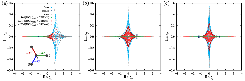
Figure 2: Visualization of the asymptotic Lefschetz thimbles for the four-site model in Eq. (32) with $K^{x}=K^{y}=0.3$, $K^{z}=0.4$, $h^{x}=0.5$, and $h^{y}=h^{z}=0$ [see the inset of (a)]. Projections onto the auxiliary variables on (a) the $x$ bond, $z_{x}$, (b) the $y$ bond, $z_{y}$, and (c) the $z$ bond, $z_{z}$ are shown. The light blue points show the time evolution of the discrete points on the real space up to $t=0.16$, which represent the flows of the asymptotic Lefschetz thimbles (corresponding to the dashed blue arrows in Fig. 1). The dark blue crosses and gray dots represent the saddle points and “zeros” (see the text for details), respectively, similar to those in Fig. 1. The green dots on the real axes represent the distribution of samples prepared by the D-QMC method in real space. The light and dark red points represent the samples on the asymptotic Lefschetz thimbles obtained at $t=0.04$ and at $t=0.08$, respectively. The average sign $S_{\mathrm{total}}$ is alleviated from $S_{\mathrm{total}}=0.7933(2)$ in the D-QMC result ($t=0$) to $S_{\mathrm{total}}=0.8155(8)$ and $S_{\mathrm{total}}=0.8304(4)$ on the asymptotic Lefschetz thimbles at $t=0.04$ and $t=0.08$, respectively. All the data are obtained for $N_{\beta}=1$ with $\beta=3.125$.

To get some insight on how the sign problem is alleviated by the ALT-QMC method, we visualize the asymptotic Lefschetz thimbles by following the time evolution explicitly. For this purpose, we adopt a simple model consisting of four sites of the Kitaev model, as shown in the inset of Fig. 2, whose Hamiltonian is given by

$$\mathcal{H}_{\mathrm{4\textnormal{-}site}}= -K^{x}\sigma_{0}^{x}\sigma_{1}^{x}-K^{y}\sigma_{0}^{y}\sigma_{2}^{y}-K^{z}\sigma_{0}^{z}\sigma_{3}^{z}$$

$$-\sum_{\gamma=x,y,z}h^{\gamma}(\sigma_{0}^{\gamma}+\sigma_{1}^{\gamma}+\sigma_{2}^{\gamma}+\sigma_{3}^{\gamma}).$$ (32)

We take a single Suzuki-Trotter slice, namely, $N_{\beta}=1$, where we have only three auxiliary variables denoted as $\varphi_{x}$, $\varphi_{y}$, and $\varphi_{z}$ on the $x$, $y$, and $z$ bonds connecting $0$-$1$, $0$-$2$, and $0$-$3$ sites, respectively. We take the parameters as $K^{x}=K^{y}=0.3$, $K^{z}=0.4$, $h^{x}=0.5$, $h^{y}=h^{z}=0$, and $\beta=3.125$. For this set up, we plot the projections of the asymptotic Lefschetz thimbles onto the complex planes of $z_{x}$, $z_{y}$, and $z_{z}$, which are obtained via the analytic continuation of the real variables $\varphi_{x}$, $\varphi_{y}$, and $\varphi_{z}$, respectively. Since in the present case the original integration domain is $\mathbb{R}^{3}$, the Lefschetz thimbles will be $\mathbb{R}^{3}$ embedded in $\mathbb{C}^{3}$, and the zeros of the fermion determinant will be $\mathbb{C}^{2}$ (see Sec. II.2). For the explicit form of the action $\mathcal{S}(\bm{z})$ derived for the model in Eq. (32) we refer to Appendix A.

First, we demonstrate the time flows of the asymptotic Lefschetz thimbles, which are schematically drawn by the dashed blue arrows in Fig. 1. For this purpose, we prepare a set of discrete points in the original integration domain $\mathbb{R}^{3}$ in the parameter range where the weight $e^{-\mathrm{Re}\mathcal{S}(\bm{\varphi})}$ has a significant value (we confirm that the numerical integration over the discrete points reproduce the value of the action with sufficient precision), and follow their time evolution calculated by Eq. (5). The results up to $t=0.16$ are shown by the light blue points in Fig. 2. The flows evolve while increasing time and appear to form envelops in a different way between the three variables $z_{x}$, $z_{y}$, and $z_{z}$. The envelops are expected to give the asymptotic Lefschetz thimbles $\mathcal{C}_{t}$, as schematically shown in Fig. 1, although the time flows may become numerically unstable at some point in practice (see below).

At the same time, we plot both the saddle points and the zeros of the fermion determinant in Fig. 2. The saddle points are obtained by solving Eq. (3) directly. They are located near the real axis in all the three projections, forming the complex conjugate pairs, as shown by the crosses in Fig. 2. The envelops of the asymptotic Lefschetz thimbles (light blue points) appear to approach the saddle points by the time evolution. Meanwhile, the zeros are obtained from the time evolution by Eq. (5) as follows. In the vicinity of zeros of the fermion determinant, the solution of Eq. (5) blows up, and hence, the numerical integration becomes unstable. We assume that the flow in Eq. (5) hits a zero when the numerical value of $\mathrm{Re}\mathcal{S}(\bm{z})$ starts to decrease or when the value of $\mathrm{Im}\mathcal{S}(\bm{z})$ starts to deviate significantly during the time evolution (we set the threshold as one percent of the previous values in the flows with each Runge-Kutta-Fehlberg adaptive step size). We show the points obtained by this procedure by the gray dots in Fig. 2. Note that not all of them are true zeros of the fermion determinant, as they may include some points where the numerical integration of Eq. (5) simply fails by technical reasons (the points at which the Runge-Kutta-Fehlberg adaptive step size becomes too small or the number of adaptive steps becomes too large are also included). In any case, the results in Fig. 2 indicate the asymptotic Lefschetz thimbles appear to be terminated in the regions where the “zeros” are densely distributed.

IV.3 Alleviation of sign problem

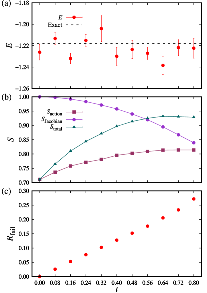
Figure 3: Flow time $t$ dependences of (a) the internal energy $E$, (b) the average sign of the action, $S_{\mathrm{action}}$ in Eq. (28), the average sign of the Jacobian, $S_{\mathrm{Jacobian}}$ in Eq. (29) and the total average sign $S_{\mathrm{total}}$ in Eq. (30), and (c) the ratio of the failed samples, $R_{\mathrm{fail}}$. The model is the four-site Kitaev model in Eq. (32) with $K^{x}=K^{y}=K^{z}=1/3$, $h^{x}=h^{y}=0$, and $h^{z}=0.2$. We take $N_{\beta}=4$ and $\beta=5$. The statistical errorbars are calculated from eight independent samples, each consisting of $5\times 10^{3}$ MC sweeps for thermalization and $9.5\times 10^{3}$ MC sweeps for measurement.

		exact		D-QMC			ALT-QMC
$N_{\beta}$		$E$		$E$	$S_{\mathrm{D\textnormal{-}QMC}}$		$E$	$S_{\mathrm{action}}$	$S_{\mathrm{total}}$
$4$		$-1.2179$		$-1.226(7)$	$0.711(3)$		$-1.229(9)$	$0.769(3)$	$0.837(2)$
$6$		$-1.1760$		$-1.181(9)$	$0.726(3)$		$-1.178(5)$	$0.799(2)$	$0.828(2)$
$8$		$-1.1612$		$-1.16(1)$	$0.736(4)$		$-1.170(9)$	$0.803(2)$	$0.818(3)$

Table 1: Comparison of the results obtained by the exact computation of the partition function in Eq. (18), the D-QMC method, and the ALT-QMC method. The model, parameters, and notations are common to those in Fig. 3, except for $N_{\beta}$. The ALT-QMC results are obtained at $t=0.22$. $S_{\mathrm{Jacobian}}\simeq 1$ for all the cases.

With the above visualization in mind, we demonstrate how the actual ALT-QMC simulations work. First, we present the distribution of the MC samples obtained by the D-QMC technique. They are distributed in the original integration domain $\mathbb{R}^{3}$, and hence, on the real axes in each projection, as shown by the green dots in Fig. 2. The total average sign in Eq. (30) is $S_{\mathrm{total}}=0.7933(2)$ for the D-QMC results. Here and hereafter, the number in the parenthesis represents the statistical error in the last digit, which is estimated by the standard error calculated from several independent MC samples, $\sigma_{\mathrm{SE}}$. In the present case, we take four independent MC samples, each having $9\times 10^{5}$ MC sweeps for measurement after $10^{5}$ MC sweeps for thermalization. Note that not all the samples are plotted in Fig. 2; only the values obtained every $2.5\times 10^{3}$ sweeps in one of four MC samples are shown for better visibility. The internal energy is estimated as $E_{\mathrm{D\textnormal{-}QMC}}=-2.7505(9)$, which reproduces well the exact value of $E_{\mathrm{exact}}=-2.75032$ within the statistical error.

Next, we show the distributions of the MC samples obtained by the ALT-QMC simulations, which correspond to the asymptotic Lefschetz thimbles $\mathcal{C}_{t}$. Figure 2 displays the results with the time evolution after $t=0.04$ and $t=0.08$ by the light and dark red dots, respectively. For these calculations we take four independent MC samples, each having $9\times 10^{4}$ MC sweeps for measurement after $10^{4}$ MC sweeps for thermalization and only the values obtained every ten sweeps in one of four MC samples are shown in Fig. 2 for better visibility. The results indicate that the asymptotic Lefschetz thimbles evolve from the real axis in each projection along the flows shown by the light blue points. As expected, the total average sign increases with $t$ as $S_{\mathrm{total}}=0.8155(8)$ and $S_{\mathrm{total}}=0.8304(4)$ for $t=0.04$ and $t=0.08$, respectively. The internal energy obtained by the ALT-QMC simulations reproduce the exact result as $E_{\mathrm{ALT\textnormal{-}QMC}}=-2.754(3)$ for $t=0.04$ and $E_{\mathrm{ALT\textnormal{-}QMC}}=-2.749(2)$ for $t=0.08$.

Let us discuss the flow time $t$ dependence in more detail, by taking $\beta=5$ and $N_{\beta}=4$, for the four-site Kitaev model in Eq. (32) with $K^{x}=K^{y}=K^{z}=1/3$, $h^{x}=h^{y}=0$, and $h^{z}=0.2$. Figure 3(a) shows the $t$ dependence of the internal energy $E$, indicating that $E$ reproduces well the exact value, shown by the horizontal dashed line, for all $t$ up to $t=0.80$ calculated here. Figure 3(b) shows the $t$ dependences of the total average sign $S_{\mathrm{total}}$ in Eq. (30), the average sign of the Jacobian, $S_{\mathrm{Jacobian}}$ in Eq. (29), and the average sign of the action, $S_{\mathrm{action}}$ in Eq. (28). We find that $S_{\mathrm{action}}$ increases with $t$ up to $t\simeq 0.64$ and then saturates to $S_{\mathrm{action}}\simeq 0.81$. We note that when there is only one Lefschetz thimble, $S_{\mathrm{action}}$ can be arbitrarily close to $1$ while increasing $t$; however, this does not hold for the case with multiple thimbles, since $\mathrm{Im}\mathcal{S}(\bm{z})$ can vary from one thimble to another. Hence, the above result suggests that there are more than one relevant thimbles in the present case. On the other hand, $S_{\mathrm{Jacobian}}$ steadily decreases from $1$ with $t$. As a consequence, $S_{\mathrm{total}}$, which includes these two contributions, steadily increases up to $t\simeq 0.64$, while it turns to decrease for larger $t$. These results show that the total sign $S_{\mathrm{total}}$ does not approach $1$ and shows a maximum at some point of the time $t$.

We also measure the ratio of the failed samples, $R_{\mathrm{fail}}$, in the MC simulations. The failed samples are the MC samples which collapse onto the zeros of the fermion determinant (or simply become unstable in the time evolution). In our simulations, we discard them and do not take into account in the MC measurement. The ratio of the failed samples denoted by $R_{\mathrm{fail}}$ is defined as the number of the failed samples divided by the total number of the initial MC samples. Figure 3(c) shows the $t$ dependence of $R_{\mathrm{fail}}$. We find that $R_{\mathrm{fail}}$ increases almost linearly with $t$, indicating that the ALT-QMC simulation loses its efficiency while increasing $t$.

Thus, in the practical ALT-QMC simulations, $S_{\mathrm{total}}$ becomes maximum at some $t$ and turns to decrease for large $t$, while $R_{\mathrm{fail}}$ monotonically increases with $t$. Hence, $t$ should be optimized to retain reasonable values of $S_{\mathrm{total}}$ and $R_{\mathrm{fail}}$ in practical simulations. The optimal value of $t$ could be determined by running test runs with small numbers of MC samples.

Next, we examine the convergence with respect to $N_{\beta}$. Table 1 summarizes the results for the same model as in Fig. 3 while varing $N_{\beta}$ from $4$ to $8$. The ALT-QMC results are obtained at $t=0.22$, where $R_{\mathrm{fail}}$ falls in the range of $0.06\lesssim R_{\mathrm{fail}}\lesssim 0.07$. We note that $R_{\mathrm{fail}}$ becomes smaller for larger $N_{\beta}$. At this relatively short flow time, $S_{\mathrm{Jacobian}}\simeq 1$ for all the cases. The results indicate that the exact values of the internal energy are well reproduced in all cases within the statistical errors. In addition, we find that the ALT-QMC method indeed improves the average sign for all $N_{\beta}$, compared to the D-QMC results. As a result, $S_{\mathrm{total}}$ in the ALT-QMC simulation is considerably larger compared to $S_{\mathrm{D\textnormal{-}QMC}}$ in the D-QMC simulation, while $S_{\mathrm{action}}$ as well as $S_{\mathrm{total}}$ is reduced gradually while increasing $N_{\beta}$. The results prove the efficiency of the ALT-QMC method.

IV.4 Benchmark

Finally, we present the benchmark of the ALT-QMC method by performing larger scale simulations. We here consider the Kitaev model in a magnetic field on an eighteen-site cluster ($N_{S}=2\times 3^{2}$) with the periodic boundary conditions. In the following, we take the parameters to retain the threefold rotational symmetry, namely, $K^{x}=K^{y}=K^{z}=1/3$ and $h^{x}=h^{y}=h^{z}=h$ because of the following reason. As discussed in Sec. IV.3, the sign problem in the ALT-QMC simulations depends on the number of the relevant thimbles and the values of $\mathrm{Im}\mathcal{S}(\bm{z})$ on each thimble; in the extreme case, when the system has only a single thimble associated with a single saddle point, one would expect a significant alleviation of the sign problem. For this reason, we first analyzed the structure of the saddle points by varying the model parameters $K^{\gamma}$ and $h^{\gamma}$. In order to identify the saddle points, we performed D-QMC simulations and solve Eq. (3) for each D-QMC sample in the real space. From this analysis, we found that the system appears to have a single saddle point for the symmetric case with $K^{x}=K^{y}=K^{z}=1/3$ and $h^{x}=h^{y}=h^{z}=h$. We note that the values of the auxiliary fields for the saddle point are the same for all the Suzuki-Trotter slices, while they vary with $h$ as well as temperature $T$. Hence, we take this symmetric parameter set for the following simulations.

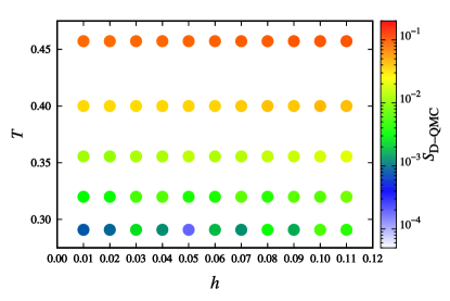
Figure 4: The average sign of the action, $S_{\mathrm{D\textnormal{-}QMC}}$ in Eq. (2), obtained by the D-QMC simulations while changing the magnetic field $h$ and temperature $T$. The results are obtained for the eighteen-site Kitaev model with $K^{x}=K^{y}=K^{z}=1/3$ and $h^{x}=h^{y}=h^{z}=h$. The average values of the sign are calculated from five independent samples, each consisting of $10^{5}$ MC sweeps for thermalization and $9\times 10^{5}$ MC sweeps for sampling. All the data are obtained for $N_{\beta}=8$.

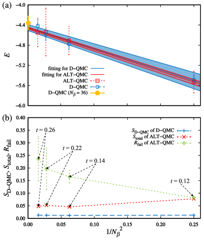
Figure 5: Benchmark results of the ALT-QMC simulations for the Kitaev model in the magnetic field. (a) The ALT-QMC results for the internal energy $E$, in comparison with the D-QMC results. The extrapolation to $N_{\beta}\to\infty$ is shown by the fitting with a linear function of $1/N_{\beta}^{2}$, plotted with the asymptotic standard errors denoted by the hatched area, for both the D-QMC and ALT-QMC data. Note that the D-QMC data at $N_{\beta}=36$ plotted by the filled orange pentagon is not incorporated in the fitting. (b) The total sign $S_{\mathrm{total}}$ in the ALT-QMC simulations, in comparison with the sign of the action, $S_{\mathrm{D\textnormal{-}QMC}}$, in the D-QMC simulations. The values of the flow time $t$ are shown in the figure. The ratio of the failed samples, $R_{\mathrm{fail}}$, is also shown. The results are obtained for the eighteen-site Kitaev model with $K^{x}=K^{y}=K^{z}=1/3$ and $h^{x}=h^{y}=h^{z}=0.04$ at $\beta=2.8125$. The statistical errorbars for the ALT-QMC results are calculated from ten independent samples, each consisting of $5\times 10^{3}$ MC sweeps for thermalization and $4.5\times 10^{4}$ MC sweeps for sampling. The statistical errorbars for the D-QMC [D-QMC ($N_{\beta}=36$)] results are calculated from ten independent samples, each consisting of $10^{5}$ ($10^{6}$) MC sweeps for thermalization and $9\times 10^{5}$ ($4\times 10^{6}$) MC sweeps for sampling. All the errorbars are presented with $\sigma_{\mathrm{SE}}$.

First of all, we show the behavior of the sign while varying $T$ and $h$ obtained by the D-QMC simulations. We find that the average sign of the action, $S_{\mathrm{D\textnormal{-}QMC}}$, decreases rapidly as $T$ decreases, as plotted in Fig. 4. The decrease is more severe in the smaller field region for $h\lesssim 0.09$. The results suggest that the D-QMC simulations become inefficient in the region below $T\simeq 0.3$ and $h\lesssim 0.09$, where $S_{\mathrm{D\textnormal{-}QMC}}$ becomes smaller than $10^{-3}$, even for this relatively small cluster with eighteen sites.

Given the D-QMC results, we perform the ALT-QMC simulations at $T=0.3\dot{5}$ ($\beta=2.8125$) and $h=0.04$, where $S_{\mathrm{D\textnormal{-}QMC}}$ is small but still retains a reasonable value of $0.013(2)$. We show the results for $N_{\beta}=2$, $4$, $6$, and $8$ in Fig. 5, in comparison with the D-QMC results which include the $N_{\beta}=36$ data. Figure 5(a) shows the internal energy $E$, as a function of $1/N_{\beta}^{2}$. We find that the results by the D-QMC and ALT-QMC methods agree with each other within the errorbars for all $N_{\beta}$. The data follows well a linear function of $1/N_{\beta}^{2}$ as expected from the discussion in Sec. III.4. The fittings are shown for both results with the confidence interval of the errors (hatched areas) estimated by a modified least-square method taking into account the errors of the data Taylor (1997). We find that the extrapolated values agree well with the result obtained by the D-QMC with sufficiently large $N_{\beta}=36$.

Figure 5(b) shows the total average sign $S_{\mathrm{total}}$ and the ratio of the failed samples, $R_{\mathrm{fail}}$, obtained by the ALT-QMC technique. We also plot the average sign of the action, $S_{\mathrm{D\textnormal{-}QMC}}$, obtained by the D-QMC technique for comparison. In the ALT-QMC simulations, we tune the flow time $t$ so that $S_{\mathrm{total}}\simeq 0.05$ for $N_{\beta}=4$, $6$, and $8$. The value of $t$ becomes larger and $R_{\mathrm{fail}}$ becomes higher for larger $N_{\beta}$, as shown in Fig. 5(b). Comparing $S_{\mathrm{total}}$ in the ALT-QMC simulations with $S_{\mathrm{D\textnormal{-}QMC}}$ in the D-QMC simulations, we find the improvement of nearly four times for all $N_{\beta}$, except for nearly six times for the $N_{\beta}=2$ case. Since the number of measurements required to obtain a constant error is proportional to $(S_{\mathrm{total}})^{-2}$, our results suggest that the performance in terms of the number of MC samples becomes nearly sixteen times higher in the ALT-QMC simulations. We note, however, that the improvement is still not enough to replace the D-QMC method at this stage, when taking into account the computational cost; the calculation complexity of the D-QMC method is $\mathcal{O}(N_{\beta}N_{S})$, which is substantially better than that of the ALT-QMC, $\mathcal{O}(N_{\beta}^{3}N_{S}^{3})$.

V Summary

To summarize, we have developed a QMC method based on the asymptotic Lefschetz thimbles that is applicable to quantum spin models with generic two-spin interactions and the Zeeman coupling to a magnetic field. The method is constructed by introducing the Hubbard-Stratonovich transformation and the Popov-Fedotov transformation. As a demonstration, we applied the method dubbed the ALT-QMC method to the Kitaev model in a magnetic field. For the four-site cluster, we visualized explicitly the time evolution of the asymptotic Lefschetz thimbles in the complex space of the auxiliary variables in the Hubbard-Stratonovich transformation, and presented how the ALT-QMC method alleviates the sign problem compared to the conventional determinant QMC method. We also showed the benchmark of the eighteen-site cluster and demonstrated the potential of studying lower-temperature regions in a magnetic field compared to the conventional method. Although the ALT-QMC method developed in the present study is still too costly, we emphasize that the average sign can be considerably improved from that in the determinant QMC method. Our results may pave the way for constructing further efficient numerical techniques.

Appendix A Explicit form of the action derived for the four site Kitaev model

The explicit form of the action $\mathcal{S}(\bm{\varphi})$ in Eq. (27) derived for the model in Eq. (32) with $h^{y}=h^{z}=0$ is expressed as

$$\mathcal{S}(\varphi_{1},\varphi_{2},\varphi_{3})=\frac{\Delta}{2}\left(\varphi_{1}^{2}+\varphi_{2}^{2}+\varphi_{3}^{2}\right)-\log\left[2\left(1+i\right)\right]$$

$$-\log\left(1+e^{-2\Delta\sqrt{K^{z}}\varphi_{3}}\right)-2\log\cosh\left(\Delta h^{x}\right)-\log\cosh\left[\Delta\left(h^{x}-\sqrt{K^{x}}\varphi_{1}\right)\right]-\log\cosh\left(\Delta\sqrt{K^{y}}\varphi_{2}\right)$$

$$-\log\left\{\left(1-ie^{2\Delta\sqrt{K^{z}}\varphi_{3}}\right)\cosh\left[\Delta\left(h^{x}-\sqrt{K^{x}}\varphi_{1}-\sqrt{K^{y}}\varphi_{2}\right)\right]+\left(-i+e^{2\Delta\sqrt{K^{z}}\varphi_{3}}\right)\cosh\left[\Delta\left(h^{x}-\sqrt{K^{x}}\varphi_{1}+\sqrt{K^{y}}\varphi_{2}\right)\right]\right\}.$$