Dependency in DAG models with Hidden Variables.

Abstract

Directed acyclic graph models with hidden variables have been much studied, particularly in view of their computational efficiency and connection with causal methods. In this paper we provide the circumstances under which it is possible for two variables to be identically equal, while all other observed variables stay jointly independent of them and mutually of each other. We find that this is possible if and only if the two variables are ‘densely connected’; in other words, if applications of identifiable causal interventions on the graph cannot (non-trivially) separate them. As a consequence of this, we can also allow such pairs of random variables have any bivariate joint distribution that we choose. This has implications for model search, since it suggests that we can reduce to only consider graphs in which densely connected vertices are always joined by an edge.

1 Introduction

Informally, a directed acyclic graph (DAG) is a collection of vertices (or nodes) joined by directed edges ($\to$) such that there is no directed path from a vertex to itself. DAGs can be used to describe Bayesian Networks by allowing each vertex to depend stochastically on its parent nodes.

We may hypothesize the existence of vertices which we cannot see, and these are referred to as hidden or latent nodes or variables.

Example 1.1.

Consider the instrumental variables model in Figure 1(a). In this case we have a DAG over four variables, of which one ($h$) is hidden. Suppose all the variables are binary, and that $H$ (the random variable associated with $h$) is Bernoulli with probability $1/2$; we select some value for $X_{a}$. Then define each of $X_{b}$ and $X_{c}$ to be an ‘xor’ gate of their two parents; we denote this addition modulo 2 using the symbol $\oplus$. Then we find that:

$$X_{b} =X_{a}\oplus H$$

$$X_{c} =X_{b}\oplus H=(X_{a}\oplus H)\oplus H=X_{a}.$$

Hence, $X_{a}=X_{c}$ with probability 1, but $X_{b}$ involves $H$, and is therefore (marginally) independent of $X_{a}$ and $X_{c}$. This is shown in Table 1, where the marginal distributions of $X_{a},X_{b}$ and of $X_{b},X_{c}$ are just the Cartesian products $\{0,1\}^{2}$, but $X_{a}=X_{c}$ for all values.

$H$	$X_{a}$	$X_{b}$	$X_{c}$
0	0	0	0
1	0	1	0
0	1	1	1
1	1	0	1

Table 1: Table showing the possible values for $X_{b}=X_{a}\oplus H$ and $X_{c}=X_{b}\oplus H$ given combinations of $X_{a}$ and $H$.

Figure 1: The instrumental variables model. (a) A directed acyclic graph on four vertices, one of which is unobserved. (b) The latent projection of this graph to an ADMG over the observed vertices.

This is a surprising result, since $X_{a}$ and $X_{c}$ do not share any edge nor a latent parent, so we might expect such a distribution not to be achievable. This can be easily extended to a sequence of bits of arbitrary cardinality, just by concatenating the values and applying the arithmetic in a bitwise fashion. In this paper we will give a generalization of this result to precisely characterize when it is possible for two variables to be equal, and independent of all other observed variables (which themselves will all be mutually independent). We will show that it is possible if and only if there is no ‘nested’ Markov constraint between the two variables in question.

1.1 Previous Work and Contribution

The question of which distributions can be realized from a directed acyclic graph model with hidden variables has been a topic of considerable interest in recent years. Its roots lie a century back in the structural diagrams of Wright (1921), later formalized as Bayesian Networks by Pearl (1986), and their Markov properties derived by Dawid, Geiger, Pearl, Lauritzen, Verma and others. Hidden variables were introduced in the 1980’s, and in this context Pearl and Verma derived the so-called ‘Verma constraint’, a constraint that is similar in form to, but distinct from, conditional independence; this restriction had been noted earlier by Robins (1986). This was later turned into an algorithm by Tian and Pearl (2002) and a nested Markov model by Richardson et al. (2017), proven algebraically complete in the discrete case by Evans (2018).

In this paper we show a different kind of completeness result for the nested Markov property to that given by Evans: approximately, we show that two vertices are ‘densely connected’ (see Definition 4.2), if and only if their associated variables can be made to be equal to one another, while remaining independent of all other observed variables. In fact, we can always reduce the nested Markov property to a maximal arid graph (MArG) in the same nested Markov equivalence class. This graph has edges precisely between densely connected vertices in the original graph, and advertises a nested constraint between every non-adjacent pair.

There are three reasons why this result is interesting. First, it gives a quick way of checking whether a particular class of distributions is compatible with a hidden variable model; this is a topic of considerable interest, particularly among computer scientists (see, e.g. Wolfe et al., 2019; Navascués and Wolfe, 2020). Second, it reinforces the importance of the nested Markov property, because it shows that it precisely characterizes when two variables can be made to have an arbitrary joint distribution, independent of all other (observed) variables. The rest of the paper is organized as follows. Finally, it suggests that we ought to restrict the class of structures that we consider in a causal model search to maximal arid graphs.

The rest of the paper is organized as follows. Section 2 gives preliminary definitions, Section 3 discusses the models and Section 4 introduces arid graphs. Then Sections 5 and 6 give our main results. Section 7 discusses finding minimal graphs, and Section 8 gives some worked examples. We end with a discussion. Code to replicate many of the analyses is contained in the R package dependence (Evans, 2021).

2 Preliminaries

In this paper we consider two classes of graph: directed acyclic graphs (DAGs), and acyclic directed mixed graphs (ADMGs). Directed acyclic graphs have a set of vertices $V$, and a collection of directed ($\to$) edges between pairs of distinct vertices. The only condition in these edges is that one cannot follow a path that coheres with the direction of the edges and end up back where one started. An ADMG is a DAG together with a collection of unordered pairs of bidirected ($\leftrightarrow$) edges. These (informally) represent hidden variables, and so are used in circumstances where one does not believe that all variables have been observed.  Note, therefore, that a DAG is an ADMG, but not the other way around in general. Examples of DAGs are given in Figures 1(a) and 2(a), and of ADMGs in Figures 1(b), 2(b), 3 and 7.

Any pair of vertices connected by an edge is said to be adjacent. A pair of vertices may be connected by either a bidirected edge or a directed edge, or both; the latter configuration is called a bow (see $b$ and $c$ in Figure 1(b), for example).

A path is a sequence of incident edges between adjacent, distinct vertices in a graph; note that two distinct paths in a mixed graph may have the same vertex set if a bow is present. The path is directed if all the edges are directed, and oriented to point away from the first vertex towards the last.

2.1 Familial Definitions

We will use standard genealogical terminology for relations between vertices. Given a vertex $v$ in an ADMG $\mathcal{G}$ with a vertex set $V$, define the sets of parents, children, ancestors, and descendants of $v$ as

$$\operatorname{pa}_{\mathcal{G}}(v) \equiv\{w:w\to v\text{ in }\mathcal{G}\}$$

$$\operatorname{ch}_{\mathcal{G}}(v) \equiv\{w:v\to w\text{ in }\mathcal{G}\}$$

$$\operatorname{an}_{\mathcal{G}}(v) \equiv\{w:w=v\text{ or }w\to\cdots\to v\text{ in }\mathcal{G}\}$$

$$\operatorname{de}_{\mathcal{G}}(v) \equiv\{w:w=v\text{ or }v\to\cdots\to w\text{ in }\mathcal{G}\},$$

respectively. These definitions also apply disjunctively to sets, e.g. for a set of vertices $C\subseteq V$, $\operatorname{pa}_{\mathcal{G}}(C)\equiv\bigcup_{v\in C}\operatorname{pa}_{\mathcal{G}}(v)$. In addition, we define the district of $v$ to be the set of vertices reachable by paths of bidirected edges:

$$\operatorname{dis}_{\mathcal{G}}(v)\equiv\{v\}\cup\{w:w\leftrightarrow\ldots\leftrightarrow v\text{ in }\mathcal{G}\}.$$

The set of districts of an ADMG $\mathcal{G}$ always partitions the set of vertices $V$. If the graph is unambiguous, we may omit the subscript $\mathcal{G}$: e.g. $X_{\operatorname{pa}(v)}$.

Given an ADMG $\mathcal{G}$, and a subset $S$ of vertices $V$ in $\mathcal{G}$, the induced subgraph $\mathcal{G}_{S}$ is the graph with vertex set $S$, and those edges in $\mathcal{G}$ between elements in $S$. A set $S\subseteq V$ is called bidirected-connected in $\mathcal{G}$ if every vertex in $S$ can be reached from every other using only a bidirected path that is contained entirely in $S$.

We sometimes abbreviate (e.g.) $\operatorname{an}_{\mathcal{G}_{S}}(v)$ and $\operatorname{dis}_{\mathcal{G}_{S}}(v)$ to $\operatorname{an}_{S}(v)$ and $\operatorname{dis}_{S}(v)$ where the graph is clear.

3 Markov Models

We consider random variables $X_{V}\equiv(X_{v}:v\in V)$ taking values in the product space ${\mathcal{X}}_{V}=\times_{v\in V}{\mathcal{X}}_{v}$, for finite dimensional sets ${\mathcal{X}}_{v}$. For any $A\subseteq V$ we denote the subset $(X_{v}:v\in A)$ by $X_{A}$. For a particular value $x_{V}\in{\mathcal{X}}_{V}$ we similarly denote a subvector over the set $A$ by $x_{A}$.

We will say that a distribution $p$ is Markov with respect to a DAG $\mathcal{G}$, if for each $v\in V$, we can write

$$X_{v}=f_{v}(X_{\operatorname{pa}_{\mathcal{G}}(v)},E_{v})$$

for some measurable function $f_{v}$, and independent noise variables $E_{v}$. That is, each variable depends on its predecessors only through the value of its direct parents in the graph. If the resulting joint distribution admits a density $p$, then this implies the usual factorization:

$$p(x_{V}) =\prod_{v\in V}p(x_{v}\mid x_{\operatorname{pa}(v)}), x_{V}\in{\mathcal{X}}_{V}.$$

This corresponds to a set of conditional independences over the space ${\mathcal{X}}_{V}$. See Lauritzen et al. (1990) for more details.

3.1 Canonical DAGs and Latent Projection

Given an ADMG $\mathcal{G}$, we define the canonical DAG, $\overline{\mathcal{G}}$ as the DAG in which each bidirected edge is replaced by a hidden variable with exactly two children, being the same vertices that were the endpoints of the bidirected edge. Note that now all bidirected edges have been replaced with two directed edges; since the directed part of the ADMG is acyclic, then certainly the resulting graph is acyclic. Hence, the canonical DAG is—as its name implies—always a DAG. For example, the DAG in Figure 1(a) is the canonical DAG for the graph in Figure 1(b), and similarly Figure 2(a) for 2(b).

Given a DAG, we can transform it into an ADMG that captures most of the causal structure by performing a latent projection. Simple examples correspond to the pairs of graphs in Figures 1 and 2, but we provide a definition and another example in the Appendix, Section B.1.

Given an ADMG $\mathcal{G}$ with vertices $V$, we define the marginal model as the set of distributions which can be realized as a margin over $X_{V}$ for distributions that are Markov with respect to the canonical DAG $\overline{\mathcal{G}}$. In doing this, we make no assumption about the statespace of the hidden variables, though for discrete models it is sufficient to have the same cardinality as all the observed variables, and in general it is both necessary and sufficient for the latent variables we use to be continuous.

We now define sets which are intrinsic for a particular ADMG. Take a set $B\subseteq V$, and set $B^{(0)}=V$; then alternately apply the operations:

$$B^{(i+1)}=\operatorname{dis}_{B^{(i)}}(B)\qquad B^{(i+2)}=\operatorname{an}_{B^{(i+1)}}(B),$$

increasing $i$ at each step. Each time we apply these steps either at least one vertex will be removed from $B^{(i)}$, or else the process will terminate at a superset of $B$, which we will denote by $\langle B\rangle_{\mathcal{G}}$. This is called the closure of $B$. If $\langle B\rangle_{\mathcal{G}}$ is bidirected-connected, then we say it is an intrinsic set, and the intrinsic closure of $B$.

For convenience we generally abbreviate $\langle\{v\}\rangle_{\mathcal{G}}$ as $\langle v\rangle_{\mathcal{G}}$, and (for example) $\operatorname{pa}_{\mathcal{G}}(\langle\{v\}\rangle_{\mathcal{G}})$ as $\operatorname{pa}_{\mathcal{G}}(\langle v\rangle)$.

4 Arid Graphs

The main result of this section is taken from Shpitser et al. (2018), and says that the nested Markov model associated with any ADMG $\mathcal{G}$ can be associated, without loss of generality, with a closely related maximal arid graph (MArG) $\mathcal{G}^{{\dagger}}$. In particular, the nested Markov models associated with $\mathcal{G}$ and $\mathcal{G}^{\dagger}$ are the same. Note that MArGs are themselves just a restricted class of ADMGs.

4.1 Arid Graphs

Definition 4.1.

Let $\mathcal{G}$ be an ADMG. We say that $\mathcal{G}$ is arid if $\langle v\rangle_{\mathcal{G}}=\{v\}$ for each $v\in V$.

The word ‘arid’ is used because it implies that the graph lacks any (non-trivial) ‘C-trees’ or ‘converging aborescences’.

Definition 4.2.

A pair of vertices $a\neq b$ in an ADMG $\mathcal{G}$ is densely connected if either $a\in\operatorname{pa}_{\mathcal{G}}(\langle b\rangle)$, or $b\in\operatorname{pa}_{\mathcal{G}}(\langle a\rangle)$, or $\langle\{a,b\}\rangle_{\mathcal{G}}$ is a bidirected-connected set.

An ADMG $\mathcal{G}$ is called maximal if every pair of densely connected vertices in $\mathcal{G}$ are adjacent.

Densely connected pairs of vertices form the nested Markov analogue of inducing paths (Verma and Pearl, 1990). The existence of an inducing path between two vertices means that (almost) no distribution that is Markov with respect to the graph will have any conditional independence between the associated variables. Analogously, a densely connected pair of vertices means that (almost) no distributions that are nested Markov with respect to the graph will have any conditional independences within any ADMG corresponding to a valid combination of intrinsic sets. In effect, a densely connected pair cannot be made independent, by any combination of conditioning and identifiable intervention operations.

As an example, note that the pair $\{a,c\}$ is densely connected in Figure 1(b), because $\operatorname{pa}_{\mathcal{G}}(\langle c\rangle)=\operatorname{pa}_{\mathcal{G}}(\{b,c\})=\{a,b\}$. Further details are given in the Appendix, Section C.

Definition 4.3.

Let $\mathcal{G}$ be an ADMG. We define its maximal arid projection as $\mathcal{G}^{{\dagger}}$, the ADMG with edges:

• $a\to b$ if and only if $a\in\operatorname{pa}_{\mathcal{G}}(\langle b\rangle)$;

• $a\leftrightarrow b$ if and only if the set $\langle\{a,b\}\rangle_{\mathcal{G}}$ is bidirected-connected, and both $a\notin\operatorname{pa}_{\mathcal{G}^{{\dagger}}}(b)$ and $b\notin\operatorname{pa}_{\mathcal{G}^{{\dagger}}}(a)$; that is, there is no directed edge between $a$ and $b$.

Note that, in particular, all directed edges in $\mathcal{G}$ are preserved in $\mathcal{G}^{\dagger}$, though some may be added if they preserve ancestral sets. Bidirected edges will be removed if connecting a vertex to something in its intrinsic closure, and added if they are required for maximality. For example, the MArG projection of the graph in Figure 2(b) adds a bidirected edge between the vertices 3 and 4. A further example is found in the Appendix, Section B.2.

Proposition 4.4 (Shpitser et al., 2018).

The maximal arid projection is arid and maximal.

Theorem 4.5 (Shpitser et al., 2018).

The nested model associated with an ADMG $\mathcal{G}$ is the same as the nested model associated with $\mathcal{G}^{{\dagger}}$.

Corollary 4.6.

Let $p$ be a distribution that is nested Markov with respect to $\mathcal{G}$. Then for $v,w\in V$ the variables $X_{v}$ and $X_{w}$ have a nested constraint between them if and only if $v$ and $w$ are not adjacent in the arid projection $\mathcal{G}^{\dagger}$.

5 Perfect Correlation

We now come to the main content of this paper.

We have already seen in Example 1.1 that it is possible for two vertices which are neither joined by an edge, nor share a latent parent, nevertheless to be perfectly correlated. We now give a slightly more complicated example of this phenomenon.

Example 5.1.

Consider the DAG in Figure 2(a). Suppose that each hidden variable ($H_{1},H_{2},H_{3}$) is again a Bernoulli random variable with probability $1/2$, and all the observed variables are again ‘xor’ gates. Then:

$$X_{a} =H_{1}\oplus H_{2} X_{b} =H_{1}\oplus H_{3}$$

$$X_{c} =X_{b}\oplus H_{2} X_{d} =X_{a}\oplus H_{3},$$

and hence $X_{c}=X_{d}=H_{1}\oplus H_{2}\oplus H_{3}$. It follows from Lemma A.1 (in Appendix A) that if $H_{1},H_{2},H_{3}$ are all independent, then so are $X_{a},X_{b},X_{c}$. Naturally, the same result also holds for $X_{a},X_{b},X_{d}$.

Figure 2: (a) A directed acyclic graph on seven vertices, three of which are unobserved. (b) The latent projection of this graph to an ADMG over the observed vertices.

Again, the result seems surprising given the lack of any form of adjacency between the vertices $c$ and $d$.

5.1 Minimal Closures

In our main result (Theorem 6.4) we will claim that it is possible to have a distribution in the marginal model of an ADMG, with two variables identical to one another and independent of all other observable variables if and only if they are densely connected. If these vertices are adjacent in the ADMG, then the result is obvious; if we have $w\to v$ then the value can be directly transmitted, and if $w\leftrightarrow v$ then the latent parent in the canonical DAG can just give the same value to both $v$ and $w$. We will show that, in fact, this can be applied much more generally.

Proposition 5.2.

Let $\mathcal{G}$ be an ADMG, and $B=\{v_{1},\ldots,v_{k}\}\subseteq V$. Then assume that $C:=\langle B\rangle_{\mathcal{G}}$ is a bidirected-connected (and hence intrinsic) set.

Now consider the following edge subgraph of $\mathcal{G}_{C}$, which we call $\widetilde{\mathcal{G}}_{C}$: the directed edges only contain a forest over $C$ that converges on $B$, and bidirected edges only contain a spanning tree over $C$. Then $\langle B\rangle_{\mathcal{G}}=C=\langle B\rangle_{\widetilde{\mathcal{G}}_{C}}$.

Proof.

Since every element of $\langle B\rangle_{\mathcal{G}}$ is an ancestor of some $v\in B$ in $\widetilde{\mathcal{G}}_{C}$, and also in the same district as everything in $B$, it is clear that the result holds. ∎

Note that this loosely defined procedure will generally lead to many different graphs, but they will always have the same total number of edges; that is, there will always be $|C|-1$ bidirected edges, and $|C|-|B|$ directed edges. However, the particular choice of the trees will affect which edges can be removed by the next result. In the Appendix (Section D) we give some algorithms for formally determining how to pick the trees in an efficient way.

Suppose we have a graph whose bidirected edges form a spanning tree, and a set of vertices $D\subseteq V$ that divides into $d$ districts. We say that $D$ is almost encapsulated in $\mathcal{G}$ if for every bidircted edge with an endpoint in $D$, the other endpoint is also in $D$, with the exception of exactly $d$ edges, one for each connected component.

Proposition 5.3.

Consider an ADMG $\mathcal{H}=\widetilde{\mathcal{G}}_{C}$ obtained by application of Proposition 5.2, and let $B=C\setminus\operatorname{pa}_{\mathcal{H}}(C)$ be the vertices without children. Suppose that there is a subset of vertices $A\subseteq C\setminus B$ such that $\operatorname{an}_{\mathcal{H}}(A)$ is almost encapsulated. Then if we remove $\operatorname{an}_{\mathcal{H}}(A)$ from the graph to obtain (say) $\widetilde{\mathcal{H}}$ we have $\langle B\rangle_{\widetilde{\mathcal{H}}}=\langle B\rangle_{\mathcal{H}}\setminus\operatorname{an}_{\mathcal{H}}(A)$.

Proof.

Since the set we remove is almost encapsulated, this means that the remaining vertices still have a spanning tree of bidirected edges. In addition, since the subset is ancestral, every remaining vertex is still an ancestor of an element of $B$. Hence we have the result given. ∎

This is a very useful result, since it will enable us to find a minimal graph which we can apply our results to. However, finding that set may be computationally difficult, as the next example illustrates.

Example 5.4.

Consider the graph in Figure 3, and suppose we wish to have $X_{v}=X_{w}$ and all other variables independent. This is clearly very easy, since there is a directed edge $w\to v$; however, we cannot reach this minimal graph all that easily by using Proposition 5.3. No set will work except for $\{c,e\}$, and we can make this problem have exponential complexity very easily (see Section D.2).

Figure 3: An ADMG which is not minimal w.r.t. $(v,w)$ but for which we cannot apply Corollary 5.5. See Example 5.4.

As a result of this problem, we present two much easier to apply corollaries.

Corollary 5.5.

Let $\mathcal{H}=\widetilde{\mathcal{G}}_{C}$ be an ADMG chosen using Proposition 5.2, and let $B=C\setminus\operatorname{pa}_{\mathcal{H}}(C)$. Suppose there is a vertex $a$ such that $\operatorname{ch}_{\mathcal{H}}(a)\neq\emptyset$, and such that $\operatorname{an}_{\mathcal{H}}(a)$ is almost encapsulated within $\mathcal{H}$.

Then we can remove $\operatorname{an}_{\mathcal{H}}(a)$ from the graph to obtain (say) $\widetilde{\mathcal{H}}$, and still have $C\setminus\operatorname{an}_{\mathcal{H}}(a)=\langle B\rangle_{\widetilde{\mathcal{H}}}$.

Proof.

This is just a special case of Proposition 5.3 with a single vertex $a$ instead of a set $A$. ∎

In a graph we say that a vertex is a leaf if it only has a single neighbour.

Corollary 5.6.

Let $\mathcal{H}=\widetilde{\mathcal{G}}_{C}$ be an ADMG chosen using Proposition 5.2, and let $B=C\setminus\operatorname{pa}_{\mathcal{H}}(C)$. If some $a\in C\setminus B$ is a leaf in both the directed and the bidirected trees, then we can remove it from the graph and still have $C\setminus\{a\}=\langle B\rangle_{\mathcal{H}_{-a}}$.

Proof.

This is just a special case of Corollary 5.5 with a single vertex acting as the set of ancestors. ∎

The complexity of identifying a minimal set using Proposition 5.3 motivates us to describe a linear time algorithm for determining the an inclusion minimal subgraph in Section 7 (see Algorithm 1).

6 Main Results

In this section we deal with our main concern, which is to show that if two vertices ($v$ and $w$) are densely connected, then we can set them to be equal, provided that all the other variables we need to set have at least the same cardinality as $X_{v}$ and $X_{w}$.

Definition 6.1.

Given a graph $\mathcal{G}$ and two vertices $v,w\in V$ that are densely connected, we define the subgraph $\mathcal{G}^{vw}$ as follows:

• if $w\in\operatorname{pa}_{\mathcal{G}}(\langle v\rangle)$ then use the induced subgraph $\mathcal{G}_{\langle v\rangle\cup\{w\}}$;

• if $v\in\operatorname{pa}_{\mathcal{G}}(\langle w\rangle)$ then take $\mathcal{G}_{\langle w\rangle\cup\{v\}}$;

• if $\langle\{v,w\}\rangle_{\mathcal{G}}$ is bidirected-connected, then take the induced subgraph $\mathcal{G}_{\langle\{v,w\}\rangle}$.

Note that it is possible that both $w\in\operatorname{pa}_{\mathcal{G}}(\langle v\rangle)$ and $\langle\{v,w\}\rangle_{\mathcal{G}}$ is bidirected-connected, in which case we have a choice about which graph to select. Typically we would prefer $\mathcal{G}_{\langle v\rangle\cup\{w\}}$, but it may be that $\mathcal{G}_{\langle\{v,w\}\rangle}$ enables us to select different variables to be used in the final distribution. Such greater flexibility could be useful in some circumstances (e.g. if one of the variables used in the directed case does not have sufficiently high cardinality).

Proposition 6.2.

Let $\mathcal{G}$ be a ADMG with $v,w\in V$ such that $w\in\operatorname{pa}_{\mathcal{G}}(\langle v\rangle)$. Then there is a distribution, Markov with respect to the canonical DAG $\overline{\mathcal{G}}$, such that $X_{v}=X_{w}$ and these are independent of all other observed variables. These other variables may be chosen to be mutually independent.

Proof.

We first assume that all variables are binary, and prove this for a single bit. The extension to multiple bits is obvious, provided that all the variables have sufficiently large cardinality. We will ignore any vertices other than those in $\langle v\rangle_{\mathcal{G}}\cup\{w\}$, since these are just set to be independent of all other random variables.

Reduce the graph to $\mathcal{G}^{vw}$ and then apply Proposition 5.2; we can then choose to remove any unnecessary variables from $\langle v\rangle_{\mathcal{G}}$ using Proposition 5.3 if we want to.

In this new smaller graph, say $\mathcal{H}$, consider the canonical DAG $\overline{\mathcal{H}}$. Set all hidden variables in $\overline{\mathcal{H}}$ to be independent Bernoulli r.v.s with parameter $1/2$, and select some arbitrary $x_{w}\in\{0,1\}$. Now, let every other observed variable, including $X_{v}$, be the sum of its parents modulo 2. There is a unique directed path that carries the value of $X_{w}$ down to $X_{v}$ (though, of course, it will generally be encoded with various additions).

Every hidden variable has exactly two children, and since these children are both ancestors of $v$ by exactly one path, this means that their value will have been cancelled out at the node where the two paths first meet. Consequently, the value of every bidirected edge will have been removed by the time we reach $v$, and so $X_{v}=x_{w}$ as required.

Now ignore $X_{w}$, and consider some subset $D\subseteq C$ of the other variables in the intrinsic closure of $v$. Remember that there is a spanning tree of bidirected edges, so in order to obtain that a set of variables is jointly dependent we always need both the endpoints of any bidirected edge. This clearly implies that we need the whole tree, and hence all of $C$; but recall that (exactly) one variable has $X_{w}$ as a parent, so therefore even the entire set $C$ consists of independent random variables. ∎

The next proposition deals with the other way in which two vertices can be densely connected.

Proposition 6.3.

Let $\mathcal{G}$ be an ADMG with $v,w\in V$ such that $\langle\{v,w\}\rangle_{\mathcal{G}}$ is bidirected-connected. Then there is a distribution, Markov with respect to the canonical DAG $\overline{\mathcal{G}}$, such that $X_{v}=X_{w}$ and these are independent of all other observed variables. Again, these variables may be chosen to be mutually independent.

Proof.

First, obtain $\mathcal{G}^{vw}$ from Definition 6.1, and then find $\mathcal{H}=\widetilde{\mathcal{G}}^{vw}$ from Proposition 5.2. Then again (optionally) choose $\langle\{v,w\}\rangle_{\mathcal{H}}$ to be minimal by applying Proposition 5.3. Then set all latent variables in $\overline{\mathcal{H}}$ to be independent Bernoulli random variables with parameter $1/2$.

Set all observed variables to be the sum modulo 2 of their parents. Now, each latent variable has two children, and by minimality of the directed edges, each of these is an ancestor of exactly one of $v$ or $w$. If both are ancestors of $v$ (or of $w$), then the value of the latent variable will cancel out at the vertex where the two descending paths meet. Otherwise, the latent variable appears in the sums for both $X_{v}$ and $X_{w}$. Hence $X_{v}=X_{w}$.

For the other variables, any subset that (possibly) includes $v$ will involve only one end of at least one bidirected edge. Hence by Lemma A.1 these variables are all independent. ∎

Note that if neither of these conditions of Propositions 6.2 or 6.3 hold, then there must be a (nonparametric) nested constraint between $X_{v}$ and $X_{w}$ (Shpitser et al., 2018).

Theorem 6.4.

We can obtain any joint distribution on $(X_{v},X_{w})$ independently of all other variables if and only if in the MArG projection there is an edge between $v$ and $w$.

Proof.

This follows from the two propositions above and the fact that if there is no edge in the MArG projection, then there is a nested constraint between $X_{v}$ and $X_{w}$ (Shpitser et al., 2018). This amounts to a marginal independence constraint when other variables are mutually independent, so it is clearly incompatible with the distribution described. ∎

Remark 6.5.

We can easily extend the result to arbitrary discrete random variables by using essentially the same method; assume that all the variables have exactly $k$ states, and set bidirected edges to be uniformly sampled from $\{0,1,\ldots,k-1\}$. If both ends of the bidirected edge are ancestors of the same vertex (e.g. $v$) then one end of the bidirected edge must subtract its value (this way that quantity will still cancel out when the two paths meet again). If the edges are ancestors of distinct vertices then both children must add the number to their total.

6.1 Arbitrary Continuous Distributions

As we have already discussed, it is also easy to extend the result to continuous random variables by using bitwise operations; suppose that the equation to determine $X_{v}$ is $X_{v}=\bigoplus_{i\in\operatorname{pa}_{\overline{\cal H}}(v)}Y_{i}$; here $Y_{i}$ can represent either an observed or a latent variable, and we have just proven that the right hand side is the same as $X_{w}$. To obtain an arbitrary joint distribution we can just replace the structural equation with $X_{v}=f(X_{w},U)$ for an independent uniform $(0,1)$ random variable $U$, and a suitable measurable function $f$ (Chentsov, 1982, Theorem 2.2). We illustrate this with the scatter plots in Figure 4, which shows data generated from the IV model in this manner, with the marginal distributions set to be standard normal and the correlation between $X_{a}$ and $X_{c}$ set to be 0.9.

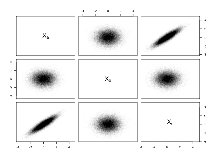
Figure 4: Scatter plot showing normal random variables simulated from the hidden variable DAG in Figure 1.

7 Algorithms for Minimality

If we have applied Proposition 5.3 as much as possible, then the graph we end up with is minimal. However, the result is not computationally efficient to use, since (in principal) we may have to try every ancestral subset of $C\setminus B$. In Algorithm 1 we give a fast algorithm to obtain a minimal set, by building it up from the two vertices $v,w$. In particular, the algorithm has worst-case linear complexity in the number of vertices.

Recall that the bidirected edges in a graph output from Proposition 5.2 are in the form of a tree, so there is a unique path between any two vertices. We denote by $\operatorname{dis}^{v}(A)$ the set of vertices on the unique bidirected paths from each $a\in A$ to $v$ (inclusive of $A$ and $v$).

Input: vertices $v,w$, graph $\mathcal{G}$ from Proposition 5.2

Result: A minimal set $W$.

1 if $w\in\operatorname{dis}_{\mathcal{G}}(v)$ then

2       initialize $A=\{v,w\}$;

3       pick $a\leftrightarrow b$ such that $a\in\operatorname{an}_{\mathcal{G}}(v)$ and $b\in\operatorname{an}_{\mathcal{G}}(w)$;

4       initialize $W=\{a,b\}\cup\operatorname{dis}^{v}(a)\cup\operatorname{dis}^{w}(b)$;

5      

6else

7       initialize $W=A=\{v,w\}$;

8      

9 end if

10while $A\neq\emptyset$ do

11       $A:=\operatorname{de}(W)\setminus W$;

12       $A:=(A\cup\operatorname{dis}^{v}(A))\setminus W$;

13       $W:=W\dot{\cup}A$;

14      

15 end while

return $W$

Algorithm 1 Find minimal set $W$ that allows $X_{v}$ and $X_{w}$ to be perfectly correlated.

Figure 5: An illustration of the construction in Proposition 6.2, for the vertices $v$ and $w$. (a) An ADMG $\mathcal{G}$, (b) its MArG projection $\mathcal{G}^{\dagger}$, and (c) its canonical DAG $\overline{\mathcal{G}}$. In (d) we reduce the directed and bidirected edges from (a) to spanning trees, as well as removing incoming edges to $z$; in (e) we remove the vertex $d$ using Corollary 5.5, and in (f) we give the canonical DAG for the graph in (e).

Figure 6: An illustration of the construction in Proposition 6.3, for the vertices $v$ and $w$. (a) An ADMG; (b) here we reduce the bidirected edges to a spanning tree; (c) we apply Corollary 5.6 to remove $c$ and take the canonical DAG.

Figure 7: (a) A graph in which it is not possible to have $X_{a}=X_{c}=X_{d}$ almost surely and independent of $X_{b}$, even though this clearly is possible in its arid projection (b).

Proposition 7.1.

The complexity of Algorithm 1 is $O(|V|)$, where $V$ is the vertex set of $\mathcal{G}$.

Proof.

Note that, since the graph consists of two trees, there are only $2(|V|-1)$ edges in total. Suppose we have the children and spouses of each vertex (otherwise we may need to run an $O(|V|)$ algorithm to obtain these, e.g. from the parent sets). Finding the district in a particular direction may involve rearranging the spouses so that the one towards $v$ (or $w$) is listed first. Again, this can be done in $O(|V|)$ time.

If the ‘if’ condition is satisfied, then we must find a bidirected edge that is an ancestor of both $v$ and $w$. These two sets can be determined in linear time, and the check for an edge will also be linear. If the ‘else’ condition is satisfied, then there is essentially nothing to do.

Then we just run the algorithm to find the descendants of $w$, or of $W$ in the ‘if’ case and then take the first entry in each list of spouses to find bidirected paths to $v$. Since we ignore any vertices that we have seen before (or stop at this point), this entire procedure will be worst case linear in the number of vertices. ∎

8 Examples

Example 8.1.

Consider the graph in Figure 5(a), and consider the pair $v,w$. Note that, in the arid projection of this graph (see (b)), there is an edge $w\to v$; hence, by Theorem 6.4, we know it must is possible to set up a distribution, Markov with respect to the canonical DAG $\overline{\mathcal{G}}$ in 5(c), such that $X_{v}=X_{w}$ and these are independent of all the other observed variables.

To do this, we simply apply Propositions 5.2 and Corollary 5.5 to obtain the graph in (e), and then follow the rules stated in the proof of Proposition 6.2. We select a value $X_{w}=x_{w}$, sample independent Bernoulli random variables for each of $H_{1}$, $H_{2}$ and $H_{3}$, and then let all other variables be xor-gates of their parents. We therefore have:

$$X_{a} =H_{1}\oplus H_{2}\qquad\qquad X_{b}=H_{1}\oplus H_{3}$$

$$X_{c} =H_{3}\oplus X_{b}\oplus x_{w}=H_{1}\oplus x_{w}$$

$$X_{v} =H_{2}\oplus X_{a}\oplus X_{c},$$

and note that by substituting in, we find:

$$X_{v} =H_{2}\oplus(H_{1}\oplus H_{2})\oplus(H_{1}\oplus x_{w})=x_{w}.$$

We also note that Lemma A.1 implies that all the other variables are independent.

Example 8.2.

Consider the graph in Figure 6(a); we can reduce this to the graph in (c) using Propositions 5.2 and 5.3. Then if we set the latent variables to be $H_{1}$, $H_{2}$, $H_{3}$ (as indicated in Figure 6(c)), we have:

$$X_{a} =H_{1}\oplus H_{2}\qquad\qquad X_{b}=H_{1}\oplus H_{3}$$

$$X_{v} =X_{a}\oplus H_{3}=H_{1}\oplus H_{2}\oplus H_{3}$$

$$\text{and}\quad X_{w} =H_{2}\oplus X_{b}=H_{2}\oplus H_{1}\oplus H_{3};$$

hence, we indeed have $X_{v}=X_{w}$. In addition, we clearly have joint independence just by applying Lemma A.1.

Note that, if we had removed the $a\leftrightarrow w$ edge when obtaining a spanning tree, we would still have been able to obtain the result. In this case everything reduces to essentially be the same as the IV model: we can remove $a$ as well as $c$, and we have $X_{v}=H_{3}$ and (if the new latent variable above $X_{b}$ and $X_{w}$ is $H_{4}$) we have $X_{w}=X_{b}\oplus H_{4}=(H_{3}\oplus H_{4})\oplus H_{4}=H_{3}$. By similar reasoning to before, the other variables $X_{a},X_{c}$ are jointly independent of each other and $X_{v}$.

Remark 8.3.

Note that the case where the arid graph induces a directed edge allows us to choose the value that the two variables take by intervening on the parent variable. However, in the case where a bidirected edge is introduced it is just a function of some hidden variables that we may not be able to control.

9 Discussion

This paper demonstrates that DAG models with hidden variables may display some surprising and counterintuitive relationships between the variables in them. In terms of causal model search, these results suggest that we may be better off restricting all ADMGs to only maximal arid graphs, since their counterparts which are not maximal and arid may exhibit spurious dependencies that do not reflect the overall structure. Note also that arid graphs are precisely those that are globally identifiable under the assumption of linear structural equations (Drton et al., 2011).

The results also provide further justification for the nested Markov model, since they show that the nested model precisely characterizes which pairs of variables can—and cannot—be made to be perfectly dependent. In other words, either two vertices possess a nested Markov constraint between them, or they can be made to be exactly equal and independent of all other variables. It also gives fast methods for checking whether certain distributions are compatible with a given hidden variable model.

9.1 Extension to multiple variables

An obvious extension to this work is to consider the possibility of simultaneously setting all $(X_{a}:a\in A)$ for some set $A\subseteq V$ to be equal, with joint independence of all other variables.

The graph in Figure 7(a) shows that the results for pairwise equality do not extend in a simple way to larger sets. Consider the triple $\{a,c,d\}$, for example. In the MArG projection of $\mathcal{G}$ (see Figure 7(b)) it clearly is possible to set these three variables to be equal, since $c,d$ are both children of $a$. However, in fact this is not possible using the canonical DAG for $\mathcal{G}$, which can be verified by applying the results of Wolfe et al. (2019) or Fraser (2020) (Elie Wolfe, personal communication.)

Acknowledgements. We thank Elie Wolfe for confirming that the graph in Figure 7(a) cannot represent the three-way perfect dependence.

Appendix A Probabilistic Result

Lemma A.1.

Consider a collection of variables $X_{1},\ldots,X_{k}$, where each $X_{i}$ is a sum modulo 2 of some subset of its predecessors, and a number of independent Bernoulli random variables with parameter $1/2$.

The Bernoulli random variables are each added to exactly two of the $X_{i}$s, and the edges induced by this graph form a tree over $\{1,\ldots,k\}$.

Then any subset of the random variables $X_{1},\ldots,X_{k-1}$ contains mutually (and jointly) independent $\operatorname{Bernoulli}(1/2)$ variables, but

$$\sum_{i=1}^{k}X_{i}=0\;\operatorname{mod}2.$$

Proof.

We proceed by induction. $X_{1}=\sum_{j\in T_{1}}Z_{j}\mod 2$ for some non-empty set $T_{1}$ of independent Bernoulli random variables, so $X_{1}$ itself must be a $\operatorname{Bernoulli}(1/2)$ r.v. Now, suppose that $X_{1},\ldots,X_{\ell-1}$ are independent $\operatorname{Bernoulli}(1/2)$ r.v.s, and consider $X_{\ell}$ for $\ell<k$. Since the random variables form a tree, then

$$X_{\ell}=\sum_{i\in S_{\ell}}X_{i}+\sum_{i\in T_{\ell}}Z_{i}\mod 2$$

is independent of $X_{1},\ldots,X_{\ell-1}$ if and only if

$$X_{\ell}^{*}:=\sum_{i\in T_{\ell}}Z_{i}\mod 2$$

is independent of $X_{1}^{*},\ldots,X_{\ell-1}^{*}$. Note, however, that since the $Z_{i}$s form a tree, there must be at least one of these variables that includes a $Z_{i}$ not seen elsewhere, so we know that this variable is independent of the rest. When we remove this variable, we then have a sub-tree, so we can repeat the argument until we have shown that all the variables are independent.

When we get to $X_{k}$ however, note that we have an invertible transformation between the $X_{i}$s and the $Z_{i}$s, and since the $Z_{i}$s form a tree over the $X_{i}$s, there is one fewer of them. It follows that the full collection of $X_{i}$s is dependent. ∎

Appendix B Graphs

The first concept we will need is an extension to ADMGs in which we allow some vertices to be ‘fixed’. We define the siblings of a vertex to be its neighbours via bidirected edges:

$$\operatorname{sib}_{\mathcal{G}}(v) \equiv\{w:v\leftrightarrow w\text{ in }\mathcal{G}\}.$$

A CADMG $\mathcal{G}(V,W)$ is an ADMG with a set of random vertices $V$ and fixed vertices $W$, with the property that $\operatorname{sib}_{\mathcal{G}}(w)\cup\operatorname{pa}_{\mathcal{G}}(w)=\emptyset$ for every $w\in W$. An example can be found in Figure 10(b); note that we depict fixed vertices with rectangular nodes, and random vertices with round nodes. Random vertices in a CADMG correspond to random variables, as in standard graphical models, while fixed vertices correspond to variables that were fixed to a specific value by some operation, such as conditioning or causal interventions. The genealogical relations in Section 2 generalize in a straightforward way to CADMGs by ignoring the distinction between $V$ and $W$; the only exception is that districts are only defined for random vertices, so that the districts in the graph partition only $V$, rather than $V\cup W$.

B.1 Latent Projection

The latent projection of a CADMG $\mathcal{G}(V\dot{\cup}L,W)$ to another graph $\mathcal{G}^{\prime}(V,W)$ is given by following the rules:

• if there is a directed path from $a\in V\cup W$ to $b\in V$, and any interior vertices are in $L$, then add $a\rightarrow b$;

• if there is a path between $a,b\in V$ without any adjacent arrowheads, and any interior vertices are in $L$, that starts and ends with an arrow at $a$ and $b$, then add $a\leftrightarrow b$.

As an example, consider the ADMG in Figure 8(a), with variable $h$ designated as latent. Then the projection of this is given by the ADMG in Figure 8(b).

Figure 8: (a) An ADMG in which $h$ is latent; (b) its latent projection over $\{a,b,c,d\}$.

B.2 Arid Projection

Example B.1.

The maximal arid projection of the ADMG $\mathcal{G}$ in Figure 9(a) is given in 9(b). In the graph (a) we have $\langle d\rangle_{\mathcal{G}}=\{b,d\}$, so $\operatorname{pa}_{\mathcal{G}}(\langle d\rangle)=\{a,b,c\}$. As a result, in (b) all these vertices are parents of $d$. In addition, $\langle\{d,e\}\rangle_{\mathcal{G}}=\{b,c,d,e\}$ which is bidirected connected, so we add the edge $d\leftrightarrow e$ into (b). All other adjacencies are as in (a).

Figure 9: (a) An ADMG $\mathcal{G}$ which is neither maximal nor arid; (b) its maximal arid projection.

Appendix C The Nested Markov Model

C.1 Fixing

A vertex $r\in V$ is said to be fixable in a CADMG $\mathcal{G}(V,W)$ if $\operatorname{dis}_{\mathcal{G}}(r)\cap\operatorname{de}_{\mathcal{G}}(r)=\emptyset$. For instance, the vertices $a$, $c$ and $d$ are all fixable in the graph in Figure 10(a), but $b$ is not because $d$ is both its descendant and its sibling.

For any $v\in V$, such that $\operatorname{ch}_{\mathcal{G}}(v)=\emptyset$, the Markov blanket of $v$ in a CADMG $\mathcal{G}$ is defined as

$$\operatorname{mb}_{\mathcal{G}}(v)\equiv(\operatorname{dis}_{\mathcal{G}}(v)\cup\operatorname{pa}_{\mathcal{G}}(\operatorname{dis}_{\mathcal{G}}(v)))\setminus\{v\};$$

that is, the set of vertices that are connected to $v$ by paths with an arrow at $v$ and two arrowheads at each internal vertex. We can generalize this definition to any vertex that is childless within its own district.

Given a CADMG $\mathcal{G}(V,W)$, and a fixable $r\in V$, the fixing operation $\phi_{r}(\mathcal{G})$ yields a new CADMG $\widetilde{\mathcal{G}}(V\setminus\{r\},W\cup\{r\})$ obtained from $\mathcal{G}(V,W)$ by removing all edges of the form $\to r$ and $\leftrightarrow r$, and keeping all other edges. Given a kernel $q_{V}(x_{V}\,|\,x_{W})$ associated with a CADMG $\mathcal{G}(V,W)$, and a fixable $r\in V$, the fixing operation $\phi_{r}(q_{V};\mathcal{G})$ yields a new kernel

$$\widetilde{q}_{V\setminus\{r\}}(x_{V\setminus\{r\}}\,|\,x_{W},x_{r})\equiv\frac{q_{V}(x_{V}\,|\,x_{W})}{q_{V}(x_{r}\,|\,x_{\operatorname{mb}_{\mathcal{G}}(r)})}.$$

A result in Richardson et al. [2017] allows us to unambiguously define

$$\phi_{R}(\mathcal{G}) \equiv\phi_{r_{k}}(\ldots\phi_{r_{2}}(\phi_{r_{1}}(\mathcal{G}))\ldots),$$

and similarly the kernel $\phi_{R}(p;\mathcal{G})$ for distributions that are nested Markov with respect to $\mathcal{G}$ (defined below). Consequently, we just use sets to index fixings from now on.

If a fixing sequence exists for a set $R\subseteq V$ in $\mathcal{G}(V,W)$, we say $V\setminus R$ is a reachable set. Such a set is called intrinsic if the vertices in $V\setminus R$ are bidirected-connected (so that $\phi_{V\setminus R}(\mathcal{G})$ has only a single district); this definition is equivalent to the definition in the main paper. We denote the collections of reachable and intrinsic sets in $\mathcal{G}$ respectively by ${\cal R}(\mathcal{G})$ and ${\cal I}(\mathcal{G})$.

For a CADMG $\mathcal{G}(V,W)$, a (reachable) subset ${C}\subseteq{V}$ is called a reachable closure for ${S}\subseteq{C}$ if the set of fixable vertices in $\phi_{V\setminus C}(\mathcal{G})$ is a subset of ${S}$. Every set ${S}$ in $\mathcal{G}$ has a unique reachable closure, which we denote $\langle S\rangle_{\mathcal{G}}$ [Shpitser et al., 2018]. Note that this set is generally a subset of what we earlier called the ‘closure’.

C.2 Nested Markov Model

We are now ready to define the nested Markov model ${\mathcal{M}}_{n}(\mathcal{G})$. Given an ADMG $\mathcal{G}$, we say that a distribution $p$ obeys the nested Markov property with respect to $\mathcal{G}$ if for any reachable set $R$, we have that $\phi_{V\setminus R}(p;\mathcal{G})$ factorizes into kernels as

$$\phi_{V\setminus R}(p;\mathcal{G}) =\prod_{D\in\mathcal{D}(\phi_{V\setminus R}(\mathcal{G}))}\phi_{V\setminus D}(p;\mathcal{G}).$$

In other words, for any reachable graph, the associated kernel factorizes into a product of the districts in that graph conditional on the parents of those districts.

Note that this also means that $\phi_{V\setminus R}(p;\mathcal{G})$ will be Markov with respect to the CADMG $\phi_{V\setminus R}(\mathcal{G})$ for each reachable set $R$; see Richardson [2003] for more details on this.

Example C.1.

Consider the ADMG in Figure 10(a). The vertices $a$, $c$ and $d$ all satisfy the condition of being fixable, but $b$ does not since $d$ is both a descendant of, and in the same district as, $b$. The CADMG $\mathcal{G}(\{b,d\},\{a,c\})$ obtained after fixing $a$ and $c$ is shown in Figure 10(b). Notice that fixing $c$ removes the edge $b\to c$, but that the edge $c\to d$ is preserved. Applying m-separation to the graph shown in Figure 10(b), yields

$$X_{d}\mathchoice{\mathrel{\hbox to0.0pt{$\displaystyle\perp$\hss}\mkern 2.0mu{\displaystyle\perp}}}{\mathrel{\hbox to0.0pt{$\textstyle\perp$\hss}\mkern 2.0mu{\textstyle\perp}}}{\mathrel{\hbox to0.0pt{$\scriptstyle\perp$\hss}\mkern 2.0mu{\scriptstyle\perp}}}{\mathrel{\hbox to0.0pt{$\scriptscriptstyle\perp$\hss}\mkern 2.0mu{\scriptscriptstyle\perp}}}X_{a}\mid X_{c}\quad[\phi_{ac}(p(x_{abcd});\mathcal{G})].$$

In addition, one can see easily that if an edge $a\to d$ had been present in the original graph, then we would not have obtained this m-separation.

Figure 10: (a) An ADMG ${\cal G}$ that is not ancestral; (b) a CADMG obtained from ${\cal G}$ in (a) by fixing $a$ and $c$.

C.3 Densely Connected Vertices

Here we give a couple of slightly more detailed examples than in the main text.

Example C.2.

The vertices $a$ and $c$ in Figure 1(b) are ‘densely connected’, because they cannot be separated by any combination of conditioning or fixing, except by fixing $c$ (which just amounts to marginalizing it from the graph). Separately, for ‘gadget’ graph in Figure 2(b) the vertices $c$ and $d$ are also ‘densely connected’. Naturally, any pair of vertices joined by an edge is also densely connected.

Appendix D Algorithms

D.1 Spanning Tree

Given a set $C$ and its subset of childless nodes $B$ (in our case this will be either $\{v\}$ or $\{v,w\}$), pick a topological order on the vertices that places all elements of $B$ at the end. Then, the last vertex before $B$ must be a parent of some element of $B$; pick the largest such element under the topological order.

We then move backwards in the topological order, and each time a vertex has more than one child, we join it to the vertex which has the shortest path to an element of $B$; if there is a tie, then we pick the largest element under the topological order. This ensures that each vertex is joined to $B$ by the shortest possible directed path.

D.2 Difficult Graphs

Consider the graph shown in Figure 11. This can clearly be reduced to the graph $w\to v$, but the application of Proposition 5.3 is computationally difficult. Note that no subset will work apart from $\{z_{1},\ldots,z_{k}\}$, and there are $3^{k}-1$ possible sets to choose.

Algorithm 1 (with complexity proven to be $O(|V|)$) can be applied instead and will immediately return the graph $w\to v$.

Figure 11: An ADMG for which a search for a set to satisfy Proposition 5.3 is computationally difficult.

References

- Chentsov [1982] N. N. Chentsov. Statistical Decision Rules and Optimal Inference. American Mathematical Society, 1982. Translated from Russian.
- Drton et al. [2011] M. Drton, R. Foygel, and S. Sullivant. Global identifiability of linear structural equation models. Annals of Statistics, 39(2):865–886, 2011.
- Evans [2018] R. J. Evans. Margins of discrete Bayesian networks. Annals of Statistics, 46(6A):2623–2656, 2018.
- Evans [2021] R. J. Evans. dependence v0.1.2, 2021. URL https://github.com/rje42/dependence. Accessed 2021-06-10.
- Fraser [2020] T. C. Fraser. A combinatorial solution to causal compatibility. Journal of Causal Inference, 8(1):22–53, 2020.
- Lauritzen et al. [1990] S. L. Lauritzen, A. P. Dawid, B. N. Larsen, and H.-G. Leimer. Independence properties of directed markov fields. Networks, 20(5):491–505, 1990.
- Navascués and Wolfe [2020] M. Navascués and E. Wolfe. The inflation technique completely solves the causal compatibility problem. Journal of Causal Inference, 8(1):70–91, 2020.
- Pearl [1986] J. Pearl. Fusion, propagation, and structuring in belief networks. Artificial Intelligence, 29:241–288, 1986.
- Richardson [2003] T. S. Richardson. Markov properties for acyclic directed mixed graphs. Scandinavial Journal of Statistics, 30(1):145–157, 2003.
- Richardson et al. [2017] T. S. Richardson, R. J. Evans, J. M. Robins, and I. Shpitser. Nested Markov properties for acyclic directed mixed graphs. arXiv:1701.06686, 2017.
- Robins [1986] J. M. Robins. A new approach to causal inference in mortality studies with sustained exposure periods – application to control of the healthy worker survivor effect. Mathematical Modeling, 7:1393–1512, 1986.
- Shpitser et al. [2018] I. Shpitser, R. J. Evans, and T. S. Richardson. Acyclic linear SEMs obey the nested Markov property. In Proceedings of the 34th Conference on Uncertainty in Artificial Intelligence (UAI-18), pages 735–745, 2018.
- Tian and Pearl [2002] J. Tian and J. Pearl. On the testable implications of causal models with hidden variables. In Proceedings of the Eighteenth Conference on Uncertainty in Artificial Intelligence (UAI-02), volume 18, pages 519–527. AUAI Press, Corvallis, Oregon, 2002.
- Verma and Pearl [1990] T. S. Verma and J. Pearl. Equivalence and synthesis of causal models. In Proceedings of the Sixth Conference on Uncertainty in Artificial Intelligence (UAI-90), 1990.
- Wolfe et al. [2019] E. Wolfe, R. W. Spekkens, and T. Fritz. The inflation technique for causal inference with latent variables. Journal of Causal Inference, 7(2), 2019.
- Wright [1921] S. Wright. Correlation and causation. Journal of Agricultural Research, 20:557–585, 1921.