Quantum Computing by Cooling

Abstract

Interesting problems in quantum computation take the form of finding low-energy states of (pseudo)spin systems with engineered Hamiltonians that encode the problem data. Motivated by the practical possibility of producing very low-temperature spin systems, we propose and exemplify the possibility to compute by coupling the computational spins to a non-Markovian bath of spins that serve as a heat sink. We demonstrate both analytically and numerically that this strategy can achieve quantum advantage in the Grover search problem.

I Introduction

Quantum computing can be implemented, conceptually, using either quantum logic gates  Grover (1996); Shor (1999); Takeshita et al. (2020); Hendrickx et al. (2020); Petit et al. (2020) or Hamiltonians  Farhi and Gutmann (1998a); Farhi et al. (2000). Under broad assumptions the two techniques are computationally equivalent, abstractly  Aharonov et al. (2007); Yu et al. (2018), but each brings in different intuitions. Roughly speaking, the gate approach is more familiar in the analysis of Turing machines and practical digital circuits, while a Hamiltonian approach is more familiar in the analysis of natural physical systems. The quantum adiabatic approach to optimization problems  Farhi et al. (2000); van Dam et al. (2001); Ozfidan et al. (2020) is an outstanding example of a class of algorithms suggested by a physical phenomenon, i.e., the preservation of quantum ground states under adiabatic evolution; other examples include algorithms inspired by resonance Wilczek et al. (2020) and diffusion Farhi and Gutmann (1998b). Physics can also suggest possibilities for resources that are not usually considered in the standard conceptual models, e.g. global addressing of qubits by external fields or controlled coupling to physically realistic heat sinks, as exemplified below.

The observation that many important computational problems can be encoded as the search for low-energy states of explicit, deceptively simple Hamiltonians $H_{\rm s}$ is central to applications of the adiabatic algorithm. One way to bring a system to low energy, of course, is to couple it to low temperature system. The production of (pseudo)spin systems with very low temperature is a highly developed art Valenzuela et al. (2006); Xu et al. (2007); Press et al. (2008); Togan et al. (2011); Yang et al. (2020). Putting those observations together, we are led to consider the possibility of addressing computational problems by coupling systems whose ground states contain the answer- “computational qubits” - to systems that have very low temperatures - “bath qubits” - that act as an energy sink.

The issue then arises, whether this procedure can be performed in a way that maintains an advantage of quantum over classical computation. Here we demonstrate that it can, at least in the context of the iconic Grover search problem Grover (1996, 1997, 1998); Nielsen and Chuang (2010).

We propose a general quantum cooling algorithm to find the ground state of a problem Hamiltonian $H_{\rm s}$. The problem system is coupled to a non-Markovian quantum bath, which is chosen to be an interacting (pseudo)spin system with trivial and easy-to-prepare ground states. As a result, the quantum bath can be readily set to the ground state. Because the bath is effectively at zero temperature, the energy will flow from the system into the bath and the problem system is cooled down to its ground state. The cooling speed of our algorithm is affected by various factors, such as the effective interaction between the system and the bath, and their energy gaps.

To show that our cooling algorithm incorporates essentially quantum features, different from classical thermal cooling van Dam et al. (2001); Farhi et al. (2002), we set up two different cooling algorithms to do random search. In the first algorithm, the coupling between the system and the bath is simple but non-local. The analytical solution shows that its time complexity is $O\left(\sqrt{N_{\rm s}}\right)$ ($N_{\rm s}$ is the dimension of the Hilbert space of $H_{\rm s}$). In the second algorithm, the coupling is local. Our analysis and numerical computation find that the time complexity is $\sim O(N_{\rm s}^{0.55})$. Both of the algorithms are faster than the classical time complexity $O(N_{\rm s})$, showing our cooling scheme is quantum coherent and different from cooling with a Markovian bath.

II Cooling with Quantum Bath

II.1 General framework

Our computing scheme involves two separate sets of qubits: computational qubits and bath qubits, for which the problem Hamiltonian $H_{\rm s}$ and the bath Hamiltonian $H_{\rm b}$ are constructed, respectively. The problem Hamiltonian $H_{\rm s}$ encodes the solutions of a given problem in its ground states. The bath Hamiltonian $H_{\rm b}$ is usually an interacting spin system with trivial ground states, so that it can be brought close to absolute zero temperature readily. For example, one may choose

$$H_{\rm b}=-J\sum_{\braket{m,m^{\prime}}}\left(\hat{\sigma}^{x}_{m}\hat{\sigma}^{x}_{m^{\prime}}+\hat{\sigma}^{y}_{m}\hat{\sigma}^{y}_{m^{\prime}}+\hat{\sigma}^{z}_{m}\hat{\sigma}^{z}_{m^{\prime}}\right)\,,$$ (1)

where $J>0$ and $\hat{\sigma}^{x,y,z}_{m}$ is the Pauli matrix of the $m$th spin. The summation is over an arbitrary set of qubit pairs $\braket{m,m^{\prime}}$. This Hamiltonian has at least two trivial ground states $\ket{00\cdots 0}$ and $\ket{11\cdots 1}$ ($\ket{0}$ for spin-down and $\ket{1}$ for spin-up), which are easy to be prepared. When the spins sit on a one-dimensional chain with the nearest neighbor interaction, it is the well-known Heisenberg XXX model Franchini (2017); Gromov et al. (2017); Salberger and Korepin (2017), and its spin wave excitation can carry energy away from the problem system Jepsen et al. (2020); Bertini et al. (2016); Castro-Alvaredo et al. (2016). There are many interacting spin systems with trivial ground states Hu et al. (2021).

The total Hamiltonian for our cooling algorithm is

$$H=H_{\rm s}+H_{\rm b}+H_{\rm I}\,,$$ (2)

where $H_{\rm I}$ is the coupling between computational qubits and bath qubits. If there are $n_{\rm s}$ computational qubits and $n_{\rm b}$ bath qubits, the Hilbert space size is $N_{\rm s}=2^{n_{\rm s}}$ for $H_{\rm s}$ and is $N_{\rm b}=2^{n_{\rm b}}$ for $H_{\rm b}$. Their energy eigen-equations are $H_{\rm s}\ket{\psi_{i_{\rm s}}}=E_{i_{\rm s}}\ket{\psi_{i_{\rm s}}}$ and $H_{\rm b}\ket{\phi_{j_{\rm b}}}=E_{j_{\rm b}}\ket{\phi_{j_{\rm b}}}$, respectively. The total Hilbert space of size $N_{\rm c}=N_{\rm s}N_{\rm b}$ is spanned by the base $\ket{\psi_{i_{\rm s}}}\otimes\ket{\phi_{j_{\rm b}}}\equiv\ket{\psi_{i_{\rm s}},\phi_{j_{\rm b}}}$. Among all $\ket{\psi_{i_{\rm s}}}$’s and $\ket{\phi_{j_{\rm b}}}$’s, for clarity, we use $\ket{g_{\rm s}}$ to denote the unknown ground states of the problem system $H_{\rm s}$ which are the solutions of the problem, and $\ket{g_{\rm b}}$ the known ground state of the bath $H_{\rm b}$ which is easy to be prepared. We set $\hbar=1$ and consider $E$ and $t$ as dimensionless variables in the following discussion because they are irrelevant to time complexity, which is our focus.

We intend to use the bath to cool down the problem system and find its ground states $\ket{g_{\rm s}}$. The bath is initialized in one of its trivial ground states, so that it is at the absolute zero temperature. The problem system can be initialized in an arbitrary state that is easy to be prepared. So, the full initial wave function at $t=0$ is

$$\ket{\Psi_{\rm in}}=\sum_{i_{\rm s}=0}^{N_{\rm s}-1}c_{i_{\rm s}}\ket{\psi_{i_{\rm s}},g_{\rm b}}\ ,$$ (3)

where $c_{i_{\rm s}}$ is the superposition probability amplitude. Once the interaction $H_{\rm I}$ is turned on, the whole composite system starts evolution with $\ket{\Psi}=e^{-iHt}\ket{\Psi_{\rm in}}$ and the energy will flow from the problem system to the bath. As a result, the problem system is cooled and will get closer to its ground state. If we measure the problem system at the end of cooling, we will have the following probability for finding the ground state $\ket{g_{\rm s}}$ of the problem system $H_{\rm s}$,

$$P_{g} = \sum_{j_{\rm b}=0}^{N_{\rm b}-1}\left|\langle g_{\rm s},\phi_{j_{\rm b}}|\Psi\rangle\right|^{2}\ .$$ (4)

The aim of our cooling algorithm is to make this probability high in a shortest time.

Here are key features of our cooling scheme.

• It is different from cooling with a Markovian thermal bath. All the processes here are quantum coherent.

• As the bath has easy-to-prepare ground states, it can be reset to zero temperature whenever it is necessary.

• Large density of states of the bath is required. Because efficient quantum transitions occur at energies corresponding to the spacing of computational levels which the final state $\ket{\psi_{i_{\rm s}^{\prime}},\phi_{j^{\prime}_{\rm b}}}$ have similar energy to the initial state $\ket{\psi_{i_{\rm s}},g_{\rm b}}$, namely, $E_{i_{\rm s}^{\prime}}+E_{j^{\prime}_{\rm b}}\approx E_{i_{\rm s}}+E_{g_{\rm b}}$. Note that in many important optimization problems the eigen-energies of $H_{\rm s}$ are integer multiples of a single parameter $\Delta$.

• The number of states in the bath should increase rapidly with energy. This encourages the bath to occupy higher energy states and absorb energy from the problem system. This is satisfied in most many-body systems, where higher energy can excite more quasi-particles. If the quasi-particles are weakly interacting, the growth is exponential.

• The total Hamiltonian is unchanged during the evolution. This helps maintain quantum coherence.

Our quantum cooling algorithm differs from the heat-bath algorithmic cooling (HBAC), quantum-circuit refrigerator (QCR) and interaction enhanced quantum computing. HBAC is used to purify a known ground state Boykin et al. (2002); Rodríguez-Briones and Laflamme (2016); Raeisi et al. (2019); Raeisi and Mosca (2015); Zaiser et al. (2021). QCR is an open system usually coupled to Markovian bath Tan et al. (2017); Silveri et al. (2017); Hsu et al. (2020). For interaction enhanced quantum computing, the interaction is between different quantum computers not between a system and a bath Shi et al. (2020). We also note that an early work indicates that non-Markovian bath could improve the performance of a quantum refrigerator Camati et al. (2020).

II.2 Toy Model

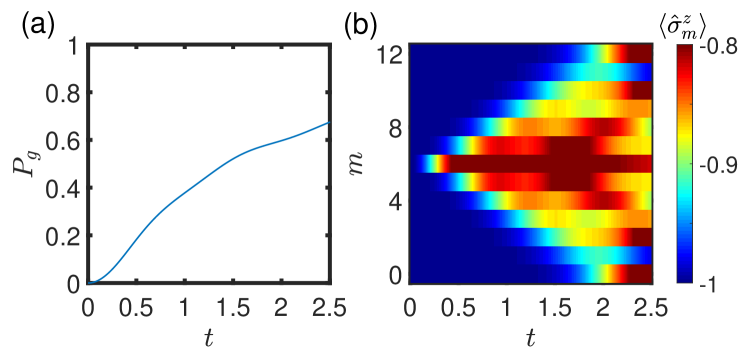
Figure 1: (color online) (a) The ground state probability of the system in Eq. (5). (b) The color is the $z$ direction component of each qubit in the bath. $m$ marks different qubits. Other parameters are $n_{\rm s}=1$, $n_{\rm b}=13$, $J=1$, $B=1$, $\lambda=1$ and $\ket{\Psi_{\rm in}}=\ket{e_{\rm s},g_{\rm b}}$.

To get oriented, let us briefly consider a toy example. The system is a single spin coupled to the middle spin of a one-dimensional spin chain,

$$H_{\rm s}=B\hat{s}^{z}\ ,\quad H_{\rm I}=\lambda\hat{s}^{y}\hat{\sigma}_{\left\lfloor\frac{n_{\rm b}}{2}\right\rfloor}^{y}\ ,$$ (5)

where $\hat{s}^{z}_{m}$ is the Pauli matrix of the system, $B$ is the on-site energy and $\lambda$ is the coupling strength. The bath is one-dimensional spin chain governed by the Hamiltonian in Eq. (1) with the nearest neighbor interaction and periodic boundary condition.

The system spin is set in the excited state and the bath is set in the ground state with all spins down. After the interaction is turned on instantaneously, the energy begins to flow into the bath, generating spin wave excitations that carry away energy from the problem system Vandaele et al. (2017); Liu et al. (2018); Bertini et al. (2016); Castro-Alvaredo et al. (2016). Numerical results are shown in Fig. 1. In Fig. 1(a), the probability of the system in the ground state becomes larger with time. Meanwhile, the energy spreads away from the middle of the chain as shown in Fig. 1(b) [see Appendix A for an analytical approach].

III Unsorted Search

Unsorted search is a benchmark example demonstrating a sharp difference between quantum and classical computers. To search $M$ targets among $N$ unsorted items, the time complexity of a classical algorithm is $O(N/M)$. In contrast, the Grover’s algorithm on a quantum computer has time complexity of $O\left(\sqrt{N/M}\right)$ Boyer et al. (1998); Giri and Korepin (2017). When our cooling algorithm is applied to this search problem, we expect a time complexity no better than $O\left(\sqrt{N_{\rm c}/N_{\rm b}}=\sqrt{N_{\rm s}}\right)$. The reason is that all the $N_{\rm b}$ states $\ket{g_{\rm s},j_{\rm b}}$’s are the targets among the total $N_{\rm c}=N_{\rm s}N_{\rm b}$ states for the whole system. We present two different cooling algorithms for unsorted search: one with non-local interaction and the other with local interaction. The first achieves the benchmark quantum time complexity $O\left(\sqrt{N_{\rm s}}\right)$ and the second comes close to that time complexity $\sim O\left(N_{\rm s}^{0.55}\right)$.

In our quantum algorithm, all the search items are stored in system qubits and represented by states $\ket{i_{\rm s}}$. In the state of $\ket{i_{\rm s}}$, the $m$th system qubit is in the state $\ket{i_{\rm s}^{(m)}}$ ($m=0,1,2,\cdots,n_{\rm s}-1$) with $i_{\rm s}^{(m)}$ being the binary digit of $i_{\rm s}$. For simplicity, we consider the case where there is only one target, $\ket{x_{\rm s}}$, which is one of the $\ket{i_{\rm s}}$’s. We construct two Hamiltonians, respectively, for the problem system and the bath as Farhi and Gutmann (1998a); van Dam et al. (2001); Roland and Cerf (2002); Wilczek et al. (2020)

$$H_{\rm s}=-\ket{g_{\rm s}}\bra{g_{\rm s}}~{}\,,~{}~{}~{}~{}~{}H_{\rm b}=-\ket{g_{\rm b}}\bra{g_{\rm b}}\ .$$ (6)

These two Hamiltonians have only two eigen-energies respectively, one for non-degenerate ground state and the other for highly-degenerate excited states (see Fig. 2). It is important to note that the system ground state $\ket{g_{\rm s}}=\ket{x_{\rm s}}$ is unknown while the bath ground state $\ket{g_{\rm b}}$ is known and can be assumed to be $\ket{g_{\rm b}}=\ket{000\cdots 0}$ without loss of generality. For the above two Hamiltonians, their energy-eigenstates are $\ket{\psi_{i_{\rm s}}}=\ket{i_{\rm s}}$ and $\ket{\phi_{j_{\rm b}}}=\ket{j_{\rm b}}$, respectively.

Our quantum algorithm is to find the system’s ground state $\ket{g_{\rm s}}$ by coupling the system to the bath and taking advantages that the bath ground state $\ket{g_{\rm b}}$ is known and easy to be prepared. Below are two quantum algorithms with different couplings, both of which outperform the classical algorithm.

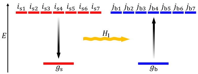
Figure 2: (color online) The diagram of the Hamiltonian $H=H_{\rm s}+H_{\rm b}+H_{\rm I}$ for unsorted search. The red bars are the energy levels of $H_{\rm s}$. The blue bars are the energy levels of $H_{\rm b}$.

III.1 Non-local Interaction

Here we choose the following non-local interaction to couple the system to the bath,

$$H_{\rm I} = -\ket{\xi}\bra{\xi}\ ,$$ (7)

where $\ket{\xi}=\sqrt{1/N_{\rm c}}\sum_{i_{\rm s}=0}^{N_{\rm s}-1}\sum_{j_{\rm b}=0}^{N_{\rm b}-1}\ket{i_{\rm s},j_{\rm b}}$. Similar non-local interactions can be found in Ref. Farhi and Gutmann (1998a); van Dam et al. (2001); Roland and Cerf (2002); Wilczek et al. (2020) and their justification can be found in Appendix B. The initial state for the whole system is

$$\ket{\Psi_{\rm in}}=\frac{1}{\sqrt{N_{\rm s}}}\sum_{i_{\rm s}=0}^{N_{\rm s}-1}\ket{i_{\rm s},g_{\rm b}}\,,$$ (8)

where the bath is in the ground state. Once the interaction is turned on, energy will flow from the problem system to the bath and the problem system will be cooled down to $\ket{g_{\rm s}}$.

For this special case, the whole cooling process is confined in a subspace spanned by the following four states,

$$\ket{Y} = \frac{1}{\sqrt{N_{\rm c}-N_{\rm s}-N_{\rm b}+1}}\sum_{i_{\rm s}=0,\atop i_{\rm s}\neq g_{\rm s}}^{N_{\rm s}-1}\sum_{j_{\rm b}=0,\atop j_{\rm b}\neq g_{\rm b}}^{N_{\rm b}-1}\ket{i_{\rm s},j_{\rm b}}\,,$$ (9)

$$\ket{\beta} = \frac{1}{\sqrt{N_{\rm b}-1}}\sum_{j_{\rm b}=0,\atop j_{\rm b}\neq g_{\rm b}}^{N_{\rm b}-1}\ket{g_{\rm s},j_{\rm b}}\,,$$ (10)

$$\ket{\alpha} = \frac{1}{\sqrt{N_{\rm s}-1}}\sum_{i_{\rm s}=0,\atop i_{\rm s}\neq g_{\rm s}}^{N_{\rm s}-1}\ket{i_{\rm s},g_{\rm b}}\,,$$ (11)

$$\ket{G} = \ket{g_{\rm s},g_{\rm b}}\,.$$ (12)

In other words, the Hamiltonian is effectively a $4\times 4$ matrix [see Appendix C]. For brevity, we just present the Hamiltonian in the limit of $1\ll N_{\rm s},N_{\rm b}\ll N_{\rm c}$

$$H \approx -\ket{Y}\bra{Y}-\ket{\alpha}\bra{\alpha}-\ket{\beta}\bra{\beta}-2\ket{G}\bra{G}$$ (13)

$$-\sqrt{\frac{N_{\rm s}}{N_{\rm c}}}\left(\ket{Y}\bra{\alpha}+\ket{\alpha}\bra{Y}\right)$$

$$-\sqrt{\frac{N_{\rm b}}{N_{\rm c}}}\left(\ket{Y}\bra{\beta}+\ket{\beta}\bra{Y}\right)\ .$$

This matrix can be diagonalized exactly. As $\ket{\Psi_{\rm in}}=\sqrt{1/N_{\rm s}}\ket{G}+\sqrt{(N_{\rm s}-1)/N_{\rm s}}\ket{\alpha}$, its time evolution is

$$\ket{\Psi}\approx e^{-2it}\sqrt{\frac{1}{N_{\rm s}}}\ket{G}+e^{-it}\sqrt{\frac{N_{\rm s}-1}{N_{\rm s}}}\left[\frac{N_{\rm s}\cos\omega t+N_{\rm b}}{N_{\rm s}+N_{\rm b}}\ket{\alpha}\right.$$

$$\left.+\frac{\sqrt{N_{\rm s}N_{\rm b}}(\cos\omega t-1)}{N_{\rm s}+N_{\rm b}}\ket{\beta}+i\sqrt{\frac{N_{\rm s}}{N_{\rm s}+N_{\rm b}}}\sin\omega t\ket{Y}\right]\,,$$ (14)

where the oscillation frequency is

$$\omega \approx \sqrt{\frac{N_{\rm s}+N_{\rm b}}{N_{\rm c}}}\ .$$ (15)

We can substitute Eq. (14) into Eq. (4) and get

$$P_{g} \approx \frac{4N_{\rm s}N_{\rm b}}{(N_{\rm s}+N_{\rm b})^{2}}\sin^{4}\frac{\omega t}{2}\ .$$ (16)

For the special case $N_{\rm b}=N_{\rm s}$, we have $P_{g}\approx 1$ at $t=\pi\sqrt{N_{\rm s}/2}$. The time complexity of our algorithm is $O(\sqrt{N_{\rm s}})$ that is as good as Grover’s Grover (1996). In general, the average time needed to finish this algorithms is

$$\overline{T}=\frac{\pi}{\max\left(P_{g}\right)_{t}\omega}=\frac{\pi\left(N_{\rm s}+N_{\rm b}\right)^{1.5}}{4\sqrt{N_{\rm s}N_{\rm b}}}\ .$$ (17)

When $N_{\rm b}=0.5N_{\rm s}$, the required time is shortest with $\overline{T}=2.04\sqrt{N_{\rm s}}$. When $N_{\rm b}\ll N_{\rm s}$, the time complexity is $O(N_{\rm s})$, which is similar to the classical algorithm. The reason is that there are not enough high energy states in a small bath to absorb energy. When $N_{\rm b}\gg N_{\rm s}$, the time complexity is $O(N_{\rm b}/\sqrt{N_{\rm s}})$ because the effective interaction becomes small. These results show that by choosing the Hamiltonians properly we can get the ground state of problem system efficiently by coupling to a quantum bath.

III.2 Local interaction

Our cooling algorithm can also achieve speed-up over the classical algorithm with local interactions. We focus on the case where the number of bath qubits $n_{\rm b}$ is the same as the computational qubits $n_{\rm s}$, i.e., $n_{\rm b}=n_{\rm s}$. The local interaction is

$$H_{\rm I}=-\lambda_{n_{\rm s}}\sum_{m=0}^{n_{\rm s}-1}\hat{s}_{m}^{x}\hat{\sigma}_{m}^{x}\ ,$$ (18)

where $\hat{s}^{x}_{m}$ and $\hat{\sigma}^{x}_{m}$ acts on the $m$th qubit of the problem system and the bath, respectively. $\lambda_{n_{\rm s}}$ is the interaction strength that $\lim_{n_{\rm s}\rightarrow\infty}\lambda_{n_{\rm s}}\times n_{\rm s}$ is a constant. It makes $\langle H_{\rm I}\rangle$ and $\langle H_{\rm s}\rangle$ the same order of magnitude. This composite system can be viewed as two parallel spin chains with pair-wise coupling (see Fig. 3).

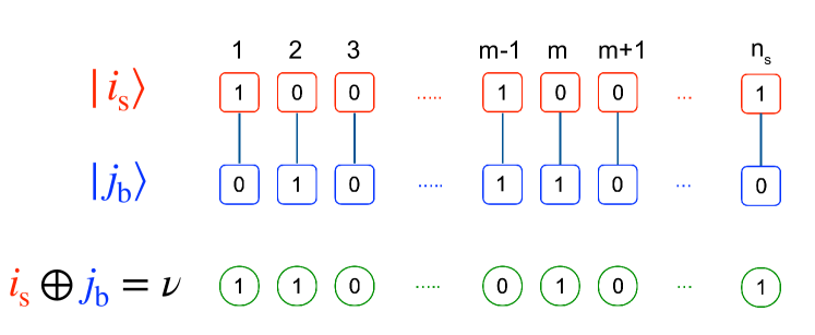
Figure 3: (color online) Illustration of $i_{\rm s}\oplus j_{\rm b}=\nu$. Red squares represent qubits of the system; blue squares represent qubits of the bath; the verticle lines represent the pair-wise interaction $\hat{s}_{m}^{x}\hat{\sigma}_{m}^{x}$ between the system qubits and bath qubits. The binary digits of $\nu$ are placed in circles for clarity.

The dynamics governed by $H$ is a unitary evolution in a Hilbert space of dimension $N_{\rm c}=N_{\rm s}N_{\rm b}=N_{\rm s}^{2}$. Fortunately, it can be decomposed into $N_{\rm s}$ independent dynamics with each of them restricted in a $N_{\rm s}$-dimensional Hilbert space. The dynamics in each of these $N_{\rm s}$-dimensional Hilbert spaces is effectively a double-well tunneling in an $n_{\rm s}$-dimensional hypercube (see Fig. 4).

This decomposition is possible due to a special property of this system, which we call parity between system qubits and bath qubits. For a pair of states $\ket{i_{\rm s}}$ and $\ket{j_{\rm b}}$, this parity is given by a number $\nu=i_{\rm s}\oplus j_{\rm b}$, where $\oplus$ is a bitwise module 2 addition as illustrated in Fig. 3 (see Appendix D for more details). Since $[\hat{s}_{m}^{z}\hat{\sigma}_{m}^{z},H]=0$, the parity number $\nu$ is conserved during the dynamical evolution.

We define a sub-Hilbert space ${\mathcal{H}}_{\nu}$, which is spanned by all $\ket{i_{\rm s},j_{\rm b}}$’s satisfying $i_{\rm s}\oplus j_{\rm b}=v$. It is easy to check that $j_{\rm b}=i_{\rm s}\oplus v$ if $v=i_{\rm s}\oplus j_{\rm b}$. This means that in each subspace ${\mathcal{H}}_{\nu}$, there is one to one mapping between the system states $\ket{i_{\rm s}}$ and the bath states $\ket{j_{\rm b}}$. Therefore, each Hilbert space ${\mathcal{H}}_{\nu}$ is of dimension $N_{\rm s}$. The subspace ${\mathcal{H}}_{\nu}$ is invariant under the unitary transformation of the total Hamiltonian $H$. As a result, the whole dynamical evolution is just a simple summation of dynamics in each subspace ${\mathcal{H}}_{\nu}$.

We still choose Eq. (8) as the initial state, where different $i_{\rm s}$’s belong to different subspaces ${\mathcal{H}}_{v_{i_{\rm s}}}$ labelled by $v_{i_{\rm s}}=i_{\rm s}\oplus g_{\rm b}$. Therefore, we can independently investigate the dynamical evolution within each subspace. In a given subspace ${\mathcal{H}}_{v_{j_{\rm s}}}$ ($j_{\rm s}$ is one of $i_{\rm s}$’s), there are only two on-site energy terms in Eq. (6) and the total Hamiltonian is reduced to

$$H_{j_{\rm s}}=-\ket{g_{\rm s},j_{\rm b}}\bra{g_{\rm s},j_{\rm b}}-\ket{j_{\rm s},g_{\rm b}}\bra{j_{\rm s},g_{\rm b}}-\lambda_{n_{\rm s}}\sum_{m=0}^{n_{\rm s}-1}\hat{s}_{m}^{x}\hat{\sigma}_{m}^{x}\ .$$

(19)

In the subspace ${\mathcal{H}}_{v_{j_{\rm s}}}$, there is one-to-one mapping between $\ket{i_{\rm s}}$ and $\ket{j_{\rm b}}$ via $i_{\rm s}\oplus j_{\rm b}=v_{j_{\rm s}}$. As a result, we can hide the bath qubits and simplify the above Hamiltonian in the subspace as

$$H_{j_{\rm s}} = -\ket{g_{\rm s}}\bra{g_{\rm s}}-\ket{j_{\rm s}}\bra{j_{\rm s}}-\lambda_{n_{\rm s}}\sum_{m=0}^{n_{\rm s}-1}\hat{s}_{m}^{x}\,.$$ (20)

The system described by this Hamiltonian can be visualized as a particle living on a hypercube of $n_{\rm s}$ dimensions (see Fig. 4(b)). Each site of this hypercube is represented by a state $\ket{i_{\rm s}}$. Only at two of these sites, $\ket{g_{\rm s}}$ and $\ket{j_{\rm s}}$, have lower on-site energy. In other words, there are two potential wells at the sites $\ket{g_{\rm s}}$ and $\ket{j_{\rm s}}$ on the hypercube and the terms $\hat{s}_{m}^{x}$ provides tunneling between them. So, it is clear that the physics in each subspace ${\mathcal{H}}_{v_{j_{\rm s}}}$ is essentially double-well tunneling in a hypercube with the initial state located at one of the wells $\ket{j_{\rm s}}$.

Figure 4: (color online) (a) One dimensional schematic illustration of Hamiltonian $H_{j_{\rm s}}$. $\ket{\chi_{g}}$ and $\ket{\chi_{j}}$ are the low energy wave packets in the wells. The combinations $(\ket{\chi_{g}}\pm\ket{\chi_{j}})/\sqrt{2}$ are the familiar ground state and the first excited state in the double-well. (b) Schematic of the $n_{\rm s}$-dimensional hypercube (placed on a hypersphere). Each point represents one configuration of qubits with the top point representing $\ket{g_{\rm s}}$. The color represents the Hamming distance $h$ of $\ket{i_{\rm s}}$ from $\ket{g_{\rm s}}$ (red for smaller distance, blue for larger distance). Yellow lines represent hopping between different $\ket{i_{\rm s}}$. (c) The actual wave function of one wave packet $\ket{\chi_{g}}$ (blue dots) reconstructed by diagonalizing Eq. (20). $\ket{j_{\rm s}}$ locates at $l_{j}=9$ for example. The number of qubits is $n_{\rm s}=18$. The interaction strength is $\gamma_{1}=1$, $\gamma_{2}=1.16$ and $\gamma_{m\geqslant 3}=0$. The calculated well component is $|a_{0}|^{2}=0.8$. The orange line is the median among same $h$.

The Hamming distance between two binary arrays is the number of bits where they differ. We define the Hamming distance between $|g_{\rm s}\rangle$ and $\ket{j_{\rm s}}$ as $l_{j}$, which ranges from 0 to $n_{\rm s}$. The dynamics in the subspaces with identical Hamming distance $l_{j}$ is exactly the same. For larger $l_{j}$, the evolution time from $|j_{\rm s}\rangle$ to $|g_{\rm s}\rangle$ is longer.

The system described by the Hamiltonian in Eq. (20) can be visualized roughly as a double-well system in Fig. 4(a). For this kind of system, the low energy Hilbert space is spanned by two wave packets $\ket{\chi_{g}}$ and $\ket{\chi_{j}}$ localized near $\ket{g_{\rm s}}$ and $\ket{j_{\rm s}}$, respectively. This is verified by our numerical computation. In our numerical computation, we expand the interaction strength in the polynomial form

$$\lambda_{n_{\rm s}} = \frac{\gamma_{1}}{n_{\rm s}}+\frac{\gamma_{2}}{n_{\rm s}^{2}}+\frac{\gamma_{3}}{n_{\rm s}^{3}}+\cdots\ .$$ (21)

We then diagonalize numerically the Hamiltonian of Eq. (20). As we expect that the two lowest eigenstates are of the form, $\left(\ket{\chi_{g}}+\ket{\chi_{j}}\right)/\sqrt{2}$ and $\left(\ket{\chi_{g}}-\ket{\chi_{j}}\right)/\sqrt{2}$ if $j\neq g$, we superpose them and obtain $\ket{\chi_{g}}$. As shown in Fig. 4(c), we find that $\ket{\chi_{g}}$ is indeed localized and its localization will not decrease as $n_{\rm s}$ increase if $\gamma_{1}\lesssim 1$ and $\gamma_{2}\lesssim 1.16$ .

The wave packet $\ket{\chi_{g}}$ can also be approximated analytically. We rearrange the basis and write $\ket{\chi_{g}}$ as

$$\ket{\chi_{g}}=\sum_{h=0}^{n_{\rm s}}\sum_{m=1}^{C_{n_{\rm s}}^{h}}a_{h,m}\ket{\psi_{h,m}},$$ (22)

where $|\psi_{h,m}\rangle$’s are re-arranged $\ket{i_{\rm s}}$’s with Hamming distance $h$ from $|g_{\rm s}\rangle$, so that $|\psi_{h=0}\rangle=|g_{\rm s}\rangle$. $m$ labels the different states with the same $h$. The $2^{n_{\rm s}}$ vertices of the hypercube can be viewed as points on the surface of an $n_{\rm s}$-dimensional hypersphere as seen in Fig. 4(b). There are $C_{n_{\rm s}}^{h}$ points locating on the same latitude of the hypersphere, which have the same $h$. When $\ket{\chi_{j}}$ is far from $\ket{\chi_{g}}$ with $l_{j}\gg 1$, the influence of $\ket{\chi_{j}}$ is so small that $\ket{\chi_{g}}$ has $n_{\rm s}$-fold rotation symmetry with the coefficients independent of $m$, i.e.,

$$a_{h,m}\approx a_{h}\ .$$ (23)

Numerically computed $a_{h,m}$ are shown in Fig. 4(c), where each blue point represents one $a_{h,m}$. It is clear from the figure that the $C_{n_{\rm s}}^{h}$ points with the same $h$ are nearly indentical. They become visibly different only near the location of $|j_{\rm s}\rangle$, i.e., at $h=9$ in this example. Most $a_{h,m}$ have the same sign except some near $|j_{\rm s}\rangle$. The interaction $\sum_{m=0}^{n_{\rm s}-1}\hat{s}_{m}^{x}$ only changes one qubit, so each point at the $h$th will interact with $h$ points at the $(h-1)$th and $n_{\rm s}-h$ points at $(h+1)$th as the yellow line shown in Fig. 4(b). If we neglect the term $-\ket{j_{\rm s}}\bra{j_{\rm s}}$ using a tight-binding approximation, the eigen-equation for Eq. (20) can be written as

$$-h\lambda_{n_{\rm s}}a_{h-1}+Va_{h}-(n_{\rm s}-h)\lambda_{n_{\rm s}}a_{h+1}=Ea_{h}\ ,$$ (24)

where $V=-1$ if $h=0$ and $V=0$ if $h\geqslant 1$. $a_{h}$ could be approached analytically using the iteration method [see Appendix E].

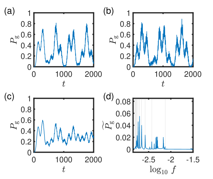
Figure 5: (color online) The evolution with Hamiltonian in Eq. (6) and Eq. (18) with $n_{\rm s}=n_{\rm b}=12$. $\gamma_{m}$ is the same as Fig. 4. $P_{g}$ is the time dependent ground state probability of the problem system. For (a) and (b), the initial condition is $\ket{\Psi_{\rm in}}=\ket{j_{\rm s},g_{\rm b}}$ with Hamming distance (a) $l_{j}=6$, (b) $l_{j}=12$. (c) The initial state is $\ket{\Psi_{\rm in}}=\sqrt{1/N_{\rm s}}\sum_{j_{\rm s}=0}^{N_{\rm s}-1}\ket{j_{\rm s},g_{\rm b}}$. (d) The Fourier transformation of (c). The gray line point out the peaks contributed by different $l_{j}$.

The two wave packets $\ket{\chi_{g}}$ and $\ket{\chi_{j}}$ have the same on-site energy. Their interaction strength decides the oscillation frequency $\omega_{l_{j}}=\left|\bra{\chi_{g}}H\ket{\chi_{j}}\right|$. In other words, $\omega_{l_{j}}$ is the evolution speed from $|j_{\rm s}\rangle$ to $|g_{\rm s}\rangle$. Physically, the interaction should decay with Hamming distance, i.e., $\omega_{l_{j}+1}<\omega_{l_{j}}$.

When the problem system evolves into $|g_{\rm s}\rangle$ through tunneling from the initial state of Eq. (8), it is cooled down by the bath and our goal is achieved. It is clear that the larger the Hamming distance $l_{j}$ the longer it takes to get $|g_{\rm s}\rangle$. The longest time occurs when $l_{j}=n_{\rm s}$. However, to have a detectable ground state probability, we just need to wait until half of the states with $l_{j}\leqslant\left\lfloor n_{\rm s}/2\right\rfloor$ evolve to $|g_{\rm s}\rangle$. The ground state probability can thus be approximated as

$$P_{g} \approx \frac{1}{N_{\rm s}}\left(A_{0}+\sum_{l=1}^{\left\lfloor\frac{n_{\rm s}}{2}\right\rfloor}C_{n_{\rm s}}^{l}A_{l}\sin^{2}\omega_{l}t\right),$$ (25)

where $t$ is in the time scale regime $1/\omega_{\left\lfloor n_{\rm s}/2\right\rfloor}<t<1/\omega_{\left\lfloor n_{\rm s}/2\right\rfloor+1}$ and $A_{l}$ is the oscillation amplitude of a scale around 1. On average, the ground state probability is

$$\overline{P_{g}} \approx \frac{\overline{A_{l}}}{N_{\rm s}}\left(1+\sum_{l=1}^{\left\lfloor\frac{n_{\rm s}}{2}\right\rfloor}C_{n_{\rm s}}^{l}\overline{\sin^{2}\omega_{l}t}\right)\approx\frac{\overline{A_{l}}}{4}\,,$$ (26)

which is large enough for detection and independent of $n_{\rm s}$.

Fig. 5(a) displays the oscillations of ground state probability with $l_{j}=\left\lfloor n_{\rm s}/2\right\rfloor$ and Fig. 5(b) shows the oscillations with $l_{j}=n_{\rm s}$. The period of (b) is larger than (a) because of longer Hamming distance. The oscillations with $l_{j}=n_{\rm s}$ has largest time scale which corresponds to the full thermal equilibrium. The evolution with the initial state Eq. (8) is shown in Fig. 5(c), where the increasing slope near $t=0$ is seen similar to (a). It indicates that the problem system can be cooled down considerably earlier before the equilibrium between the bath and problem system is reached. Fig. 5(d) is the Fourier transformation of (c). You can clearly see the peaks for independent oscillations with different $l_{j}$.

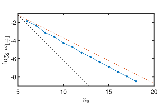
Figure 6: (color online) The oscillation frequency between $|j_{\rm s}\rangle$ and $|g_{\rm s}\rangle$ with distance $l_{j}=\left\lfloor n_{\rm s}/2\right\rfloor$ according to Eq. (20). The blue dots are the exact value from diagonalization whose slop is about -0.55. $\gamma_{m}$ is the same as Fig. 4. The slope of the orange dash line is -0.5 representing Grover’s algorithm. The slope of the black dash line is -1 representing the classical algorithm.

The oscillation frequency $\omega_{l_{j}}$ is decided by the energy difference of two lowest energy states in the subspace. The cooling speed is about $\omega_{\left\lfloor n_{\rm s}/2\right\rfloor}$. Fig. 6 shows the dependence of the cooling speed on the number of qubits $n_{\rm s}$. It is calculated by numerical diagonalizing Eq. (20) with $l_{j}=\left\lfloor n_{\rm s}/2\right\rfloor$. By fitting the numerical result, we find that the cooling speed is about $O(N_{\rm s}^{0.55})$ with local interaction, which is close to the Grover’s algorithm Grover (1996). The form of interaction does not strongly affect the cooling speed.

IV Discussion and Conclusion

We have proposed a general framework of quantum computing by cooling a Hamiltonian system whose ground states encode the solutions of a given problem with a fully quantum (non-Markovian) bath. This bath, which could be called a quantum icebox, is an interacting spin system with trivial and easy-to-prepare ground states so that it can be brought close to absolute zero temperature readily. We illustrated this method in two specific realizations in the benchmark problem of unsorted search. In both cases, we found a strong quantum advantage.

It is appropriate to contrast our work with the more familiar quantum adiabatic algorithm (QAA) or quantum annealing Johnson et al. (2011); McGeoch (2014); Qiu et al. (2020). In QAA, the system with simple Hamiltonian is set to its simple ground state (effectively absolute zero temperature), and it is then slowly changed (or annealed) to another more complicated Hamiltonian, whose ground states are the solutions of a given problem Farhi et al. (2001); Lucas (2014). In the whole process, the system is vulnerable to external heat or noise Paladino et al. (2014); Bilmes et al. (2017); Braumüller et al. (2020) and often encounters exponentially small energy gap Young et al. (2008). In our framework, the quantum icebox can be made large enough to offer two advantages: (1) to make sure the quantum icebox does not heat up before the system cools down; (2) to protect the system from decoherence. Given that a functioning quantum computer has already been built based QAA Harris et al. (2010); Johnson et al. (2011), our icebox strategy seems likely to be practicable. Specifically, the experimental systems used to implement QAA and quantum simulation (QS) Monroe et al. (2021); Ebadi et al. (2021) can be modified to explore this possibility.

Heat transfer has long been regarded as a stochastic thermal process He et al. (1998); Wang et al. (2008); Sääskilahti et al. (2013). Our quantum icebox shows that cooling can be done coherently. It raises fresh questions about the connection between heat transport and the flow of quantum information.

Appendix A Analytical result of spin wave propagation

The spin wave dynamics with total Hamiltonian $H=H_{\rm s}+H_{\rm b}+H_{\rm I}$ of Eq. (1) and (5) is illustrated numerically in Fig. 1. It can also be demonstrated in the single excited mode approximation, where we consider just states $\ket{e_{\rm s},k_{g}}$ and $\ket{g_{\rm s},k}$, neglecting the states with multi-magnon. $\ket{g_{\rm s}}$ and $\ket{e_{\rm s}}$ represents the excited state and ground state of the problem system, $\ket{k_{g}}$ and $\ket{k}$ represent the ground state and the excited states of the bath with wave vector $k$. The Hamiltonian becomes

$$H = \sum_{k\neq k_{g}}\big{[}\Delta E_{k}\ket{g_{\rm s},k}\bra{g_{\rm s},k}$$ (27)

$$+\lambda_{k}\ket{g_{\rm s},k}\bra{e_{\rm s},k_{g}}+\lambda_{k}^{*}\ket{e_{\rm s},k_{g}}\bra{g_{\rm s},k}\big{]}\ ,$$

where $\Delta E_{k}=\left(E_{{\rm s}g}+E_{{\rm b}k}\right)-\left(E_{{\rm s}e}+E_{{\rm b}k_{g}}\right)$ is the energy detuning and $\lambda_{k}$ is the coupling strength. The time dependent wave function is

$$\ket{\Psi} = b_{g}\ket{e_{\rm s},k_{g}}+\sum_{k\neq k_{g}}b_{k}\ket{g_{\rm s},k}\ ,$$ (28)

where the probability amplitude satisfies the Schrödinger equation with

$$\left\{\begin{array}[]{ccc}i\frac{{\rm d}b_{g}}{{\rm d}t}&=&\sum_{k\neq k_{g}}\lambda_{k}^{*}b_{k}\\ i\frac{{\rm d}b_{k}}{{\rm d}t}&=&\Delta E_{k}b_{k}+\lambda_{k}b_{g}\end{array}\right.\ .$$ (31)

In the early time of evolution $|\lambda_{k}|t\rightarrow 0$, $b_{g}\approx 1$. We can decouple the equations and get Zhang and Liu (2016)

$$b_{k} \approx \frac{\lambda_{k}}{\Delta E_{k}}\left(e^{-i\Delta E_{k}t}-1\right)\ .$$ (32)

The probability amplitude for the two level system in its excited state is

$$b_{g} \approx 1-2\sum_{k\neq k_{g}}\frac{|\lambda_{k}|^{2}}{\Delta E_{k}^{2}}\sin^{2}\frac{\Delta E_{k}t}{2}$$ (33)

In the position coordinate, the wave function is

$$\phi \approx b_{g}e^{ik_{g}x}+\sum_{k\neq k_{g}}b_{k}e^{ikx}\ .$$ (34)

The phase difference between different $b_{k}$ changes with time, the wave function will spread out from $x=0$.

Appendix B Non-locality of Hamiltonians

The Hamiltonians used in quantum algorithms must be physically reasonable. This usually means that the Hamiltonian are $k$-local, i.e., contain only interactions involving no more than a fixed number $k$ of qubits Aharonov et al. (2007). Although the three Hamiltonians in Eqs. (6,7) are not $k$-local, they are physically reasonable, and here is the explanation.

In the Grover’s algorithm, a single Grover iteration is $U_{\rm G}=R_{\xi}R_{g}$ Nielsen and Chuang (2010). $R_{g}=\mathbb{I}-2\ket{g}\bra{g}$ is the oracle operator for the target $\ket{g}$. And $R_{\xi}=H_{\rm a}^{\otimes n}\left(\mathbb{I}-2\ket{0}\bra{0}\right)H_{\rm a}^{\otimes n}=\mathbb{I}-2\ket{\xi}\bra{\xi}$, where $H_{\rm a}$ is the Hadamard gate and $\ket{\xi}=\sqrt{1/N}\sum_{j=0}^{N-1}\ket{j}$.

That the Hamiltonians in Eqs. (6,7) are reasonable despite being non-local is because the dynamics generated by them can be implemented with the Grover operation $U_{\rm G}$. For simplicity, we consider the Hamiltonian dynamics $U=e^{-iHt}$ with $H=-\ket{g}\bra{g}-\ket{\xi}\bra{\xi}$. When the time evolution is discretized with time step $\Delta t=\pi$ and $T=m\Delta t$, we have Mochon (2007)

$$U=e^{-iHT}\approx\Pi_{j=1}^{m}e^{-i\pi H}\approx\Pi_{j=1}^{m}U_{\rm G}\ .$$ (35)

Note that the circuit complexity for implementing the oracle is $O\left(n^{3}\right)$ Tanaka et al. (2011) and the time complexity is $O\left(n^{2}\right)$ Ito and Iida (2014), where $n=\log_{2}N$.

Appendix C Exact Hamiltonian for the non-local model

We expand the total Hamiltonian $H=H_{\rm s}+H_{\rm b}+H_{\rm I}$ of Eq. (6) and (7) in terms of $\ket{Y}$, $\ket{\beta}$, $\ket{\alpha}$, $\ket{G}$ of Eqs. (9), (10), (11) and (12). Its exact matrix is

$$H=-\frac{1}{N_{\rm c}}\left(\begin{smallmatrix}N_{\rm c}-N_{\rm s}-N_{\rm b}+1&\sqrt{(N_{\rm c}-N_{\rm s}-N_{\rm b}+1)(N_{\rm b}-1)}&\sqrt{(N_{\rm c}-N_{\rm s}-N_{\rm b}+1)(N_{\rm s}-1)}&\sqrt{N_{\rm c}-N_{\rm s}-N_{\rm b}+1}\\ \sqrt{(N_{\rm c}-N_{\rm s}-N_{\rm b}+1)(N_{\rm b}-1)}&N_{\rm c}+N_{\rm b}-1&\sqrt{(N_{\rm s}-1)(N_{\rm b}-1)}&\sqrt{N_{\rm b}-1}\\ \sqrt{(N_{\rm c}-N_{\rm s}-N_{\rm b}+1)(N_{\rm s}-1)}&\sqrt{(N_{\rm s}-1)(N_{\rm b}-1)}&N_{\rm c}+N_{\rm s}-1&\sqrt{N_{\rm s}-1}\\ \sqrt{N_{\rm c}-N_{\rm s}-N_{\rm b}+1}&\sqrt{N_{\rm b}-1}&\sqrt{N_{\rm s}-1}&2N_{\rm c}+1\end{smallmatrix}\right)\ .$$ (36)

If we just keep the leading terms in the limit of $1\ll N_{\rm s},N_{\rm s}\ll N_{\rm c}$, it recovers Eq. (13) in the main text. Its eigen-energies are

$$E_{3} = -1+\sqrt{\frac{N_{\rm s}+N_{\rm b}}{N_{\rm c}}}\ ,$$ (37)

$$E_{2} = -1\ ,$$ (38)

$$E_{1} = -1-\sqrt{\frac{N_{\rm s}+N_{\rm b}}{N_{\rm c}}}\ ,$$ (39)

$$E_{0} = -2\ .$$ (40)

The eigen-states are

$$\ket{\Psi_{0}} = \begin{pmatrix}[1.8]0\\ 0\\ 0\\ 1\end{pmatrix}\,,~{}\ket{\Psi_{1}}=\begin{pmatrix}[1.8]\frac{1}{\sqrt{2}}\\ \sqrt{\frac{N_{\rm s}}{2(N_{\rm s}+N_{\rm b})}}\\ \sqrt{\frac{N_{\rm b}}{2(N_{\rm s}+N_{\rm b})}}\\ 0\end{pmatrix}\ ,$$ (41)

$$\ket{\Psi_{2}} = \begin{pmatrix}[1.8]0\\ -\sqrt{\frac{N_{\rm b}}{N_{\rm s}+N_{\rm b}}}\\ \sqrt{\frac{N_{\rm s}}{N_{\rm s}+N_{\rm b}}}\\ 0\end{pmatrix}\ ,~{}\ket{\Psi_{3}}=\begin{pmatrix}[1.8]-\frac{1}{\sqrt{2}}\\ \sqrt{\frac{N_{\rm s}}{2(N_{\rm s}+N_{\rm b})}}\\ \sqrt{\frac{N_{\rm b}}{2(N_{\rm s}+N_{\rm b})}}\\ 0\end{pmatrix}\ .$$ (42)

The time dependent wave function with initial condition $\ket{\Psi_{\rm in}}=\sqrt{1/N_{\rm s}}\ket{G}+\sqrt{(N_{\rm s}-1)/N_{\rm s}}\ket{\alpha}$ is

$$\ket{\Psi}=e^{-iE_{0}t}\sqrt{\frac{1}{N_{\rm s}}}\ket{\Psi_{0}}+$$

$$\sqrt{\frac{N_{\rm s}-1}{N_{\rm s}}}\frac{\sqrt{\frac{N_{\rm s}}{2}}\left(e^{-iE_{3}t}\ket{\Psi_{3}}+e^{-iE_{1}t}\ket{\Psi_{1}}\right)-e^{-iE_{2}t}\sqrt{N_{\rm b}}\ket{\Psi_{2}}}{\sqrt{N_{\rm s}+N_{\rm b}}}\ .$$

Expanding it, we will get Eq. (14) in the main text.

Appendix D Exclusive-OR (XOR)

The module 2 addition ”$\oplus$” is also called XOR operation for two Boolean variables, which is defined as $0\oplus 0=1\oplus 1=0$ and $0\oplus 1=1\oplus 0=1$. For an integer $i$, its binary digits $i^{(m)}$’s are defined as

$$i=\sum_{m=0}^{n-1}2^{m}i^{(m)}\ .$$ (44)

For any two integers $i_{a}$ and $j_{b}$, $v=i_{a}\oplus j_{b}$ is defined bitwise as,

$$v^{(m)}=i_{a}^{(m)}\oplus j_{b}^{(m)}\ .$$ (45)

It also can be written as

$$v=i_{a}\oplus j_{b}=\sum_{m=0}^{n-1}2^{m}\left(i_{a}^{(m)}\oplus j_{b}^{(m)}\right)\ .$$ (46)

For example $12\oplus 10=1100\oplus 1010=0110=6$. There is an inverse relation that $j_{b}=i_{a}\oplus v$ if $v=i_{a}\oplus j_{b}$. We can check that $12\oplus 6=1100\oplus 0110=1010=10$.

Appendix E Analytic approximation of the wave packet $\ket{\chi_{g}}$

Eq. (24) can be approached analytically. We re-write it as

$$\left\{\begin{array}[]{l}(-1-E)a_{0}-n_{\rm s}\lambda a_{1}=0\\ -h\lambda a_{h-1}-Ea_{h}-(n_{\rm s}-h)\lambda a_{h+1}=0\ (1\leqslant h\leqslant n_{\rm s})\end{array}\right.\ .$$ (49)

We define the ratio $b_{h}=a_{h}/a_{h-1}$ and get

$$b_{h}=\frac{h\lambda}{1+n_{\rm s}\lambda b_{1}-(n_{\rm s}-h)\lambda b_{n+1}}\ .$$ (50)

With the self-consistent method, the above iteration becomes

$$b_{h}^{(m+1)}=\frac{h\lambda}{1+n_{\rm s}\lambda b_{1}^{(m)}-(n_{\rm s}-h)\lambda b_{h+1}^{(m)}}\ ,$$ (51)

where the superscript is the order of approximation. If we set $b_{h}^{(0)}=0$, we get

$$b_{h}^{(1)} = h\lambda\ ,$$ (52)

$$b_{h}^{(2)} = \frac{h\lambda}{1+n_{\rm s}\lambda^{2}-(n_{\rm s}-h)(h+1)\lambda^{2}}\ ,$$ (53)

$$b_{h}^{(3)} = \frac{h\lambda}{1+\frac{n_{\rm s}\lambda^{2}}{1-(n_{\rm s}-2)\lambda^{2}}-\frac{(n_{\rm s}-h)(h+1)\lambda^{2}}{1+n_{\rm s}\lambda^{2}-(n_{\rm s}-h-1)(h+2)\lambda^{2}}}\ .$$ (54)

The corresponding energy is

$$E^{(1)} = -1-n_{\rm s}\lambda^{2}\ ,$$ (55)

$$E^{(2)} = -1-\frac{n_{\rm s}\lambda^{2}}{1-(n_{\rm s}-2)\lambda^{2}}\ ,$$ (56)

$$E^{(3)} = -1-\frac{n_{\rm s}\lambda^{2}}{1+\frac{n_{\rm s}\lambda^{2}}{1-(n_{\rm s}-2)\lambda^{2}}-\frac{2(n_{\rm s}-1)\lambda^{2}}{1-(2n_{\rm s}-6)\lambda^{2}}}\ .$$ (57)

We define $a_{0}=1/\sqrt{\aleph}$, where $\aleph$ is the normalization factor. The coefficient for $h\geqslant 1$ is

$$a_{h} = \frac{1}{\sqrt{\aleph}}\prod_{m=1}^{h}b_{m}\ .$$ (58)

The first order approximation is

$$a_{h}^{(1)}=\frac{1}{\sqrt{\aleph^{(1)}}}\frac{h!}{n_{\rm s}^{h}}\approx\sqrt{\frac{2\pi h}{\aleph^{(1)}}}\left(\frac{h}{en_{\rm s}}\right)^{h}\,,$$ (59)

where the last term is obtained with the Stirling approximation. It is accurate only in the regime $h\geqslant 1$ and $h/n_{\rm s}<0.2$. By fitting the numerical data in Fig. 4(c), we find that the decay speed of $a_{h}$ is exponential in the regime $h/n_{\rm s}<0.2$ and inversely proportional to $h$ in the regime $h/n_{\rm s}>0.3$.

References

- Grover (1996) L. K. Grover, in Proceedings of the Twenty-Eighth Annual ACM Symposium on Theory of Computing (Association for Computing Machinery, New York, NY, USA, 1996), STOC ’96, pp. 212–219.
- Shor (1999) P. W. Shor, SIAM Rev. 41, 303 (1999).
- Takeshita et al. (2020) T. Takeshita, N. C. Rubin, Z. Jiang, E. Lee, R. Babbush, and J. R. McClean, Phys. Rev. X 10, 011004 (2020).
- Hendrickx et al. (2020) N. W. Hendrickx, D. P. Franke, A. Sammak, G. Scappucci, and M. Veldhorst, Nature 577, 487 (2020), ISSN 1476-4687.
- Petit et al. (2020) L. Petit, H. G. J. Eenink, M. Russ, W. I. L. Lawrie, N. W. Hendrickx, S. G. J. Philips, J. S. Clarke, L. M. K. Vandersypen, and M. Veldhorst, Nature 580, 355 (2020).
- Farhi and Gutmann (1998a) E. Farhi and S. Gutmann, Phys. Rev. A 57, 2403 (1998a).
- Farhi et al. (2000) E. Farhi, J. Goldstone, S. Gutmann, and M. Sipser, Quantum computation by adiabatic evolution (2000), eprint 0001106.
- Aharonov et al. (2007) D. Aharonov, W. van Dam, J. Kempe, Z. Landau, S. Lloyd, and O. Regev, SIAM J. Comput. 37, 166 (2007).
- Yu et al. (2018) H. Yu, Y. Huang, and B. Wu, Chin. Phys. Lett. 35, 110303 (2018).
- van Dam et al. (2001) W. van Dam, M. Mosca, and U. Vazirani, in Proceedings 42nd IEEE Symposium on Foundations of Computer Science (2001), pp. 279–287.
- Ozfidan et al. (2020) I. Ozfidan, C. Deng, A. Smirnov, T. Lanting, R. Harris, L. Swenson, J. Whittaker, F. Altomare, M. Babcock, C. Baron, et al., Phys. Rev. Applied 13, 034037 (2020), URL https://link.aps.org/doi/10.1103/PhysRevApplied.13.034037.
- Wilczek et al. (2020) F. Wilczek, H.-Y. Hu, and B. Wu, Chin. Phys. Lett. 37, 050304 (2020).
- Farhi and Gutmann (1998b) E. Farhi and S. Gutmann, Phys. Rev. A 58, 915 (1998b).
- Valenzuela et al. (2006) S. O. Valenzuela, W. D. Oliver, D. M. Berns, K. K. Berggren, L. S. Levitov, and T. P. Orlando, Science 314, 1589 (2006), ISSN 0036-8075, URL https://science.sciencemag.org/content/314/5805/1589.
- Xu et al. (2007) X. Xu, Y. Wu, B. Sun, Q. Huang, J. Cheng, D. G. Steel, A. S. Bracker, D. Gammon, C. Emary, and L. J. Sham, Phys. Rev. Lett. 99, 097401 (2007), URL https://link.aps.org/doi/10.1103/PhysRevLett.99.097401.
- Press et al. (2008) D. Press, T. D. Ladd, B. Zhang, and Y. Yamamoto, Nature 456, 218 (2008), ISSN 1476-4687, URL https://doi.org/10.1038/nature07530.
- Togan et al. (2011) E. Togan, Y. Chu, A. Imamoglu, and M. D. Lukin, Nature 478, 497 (2011), ISSN 1476-4687, URL https://doi.org/10.1038/nature10528.
- Yang et al. (2020) B. Yang, H. Sun, C.-J. Huang, H.-Y. Wang, Y. Deng, H.-N. Dai, Z.-S. Yuan, and J.-W. Pan, Science 369, 550 (2020), ISSN 0036-8075, URL https://science.sciencemag.org/content/369/6503/550.
- Grover (1997) L. K. Grover, Phys. Rev. Lett. 79, 325 (1997).
- Grover (1998) L. K. Grover, Phys. Rev. Lett. 80, 4329 (1998).
- Nielsen and Chuang (2010) M. A. Nielsen and I. L. Chuang, Quantum Computation and Quantum Information: 10th Anniversary Edition (Cambridge University Press, 2010).
- Farhi et al. (2002) E. Farhi, J. Goldstone, and S. Gutmann, Quantum adiabatic evolution algorithms versus simulated annealing (2002), eprint 0201031.
- Franchini (2017) F. Franchini, An Introduction to Integrable Techniques for One-Dimensional Quantum Systems (Springer, Cham, 2017).
- Gromov et al. (2017) N. Gromov, F. Levkovich-Maslyuk, and G. Sizov, J. High Energ. Phys 2017, 111 (2017).
- Salberger and Korepin (2017) O. Salberger and V. Korepin, Rev. Math. Phys. 29, 1750031 (2017).
- Jepsen et al. (2020) P. N. Jepsen, J. Amato-Grill, I. Dimitrova, W. W. Ho, E. Demler, and W. Ketterle, Nature 588, 403 (2020).
- Bertini et al. (2016) B. Bertini, M. Collura, J. De Nardis, and M. Fagotti, Phys. Rev. Lett. 117, 207201 (2016), URL https://link.aps.org/doi/10.1103/PhysRevLett.117.207201.
- Castro-Alvaredo et al. (2016) O. A. Castro-Alvaredo, B. Doyon, and T. Yoshimura, Phys. Rev. X 6, 041065 (2016), URL https://link.aps.org/doi/10.1103/PhysRevX.6.041065.
- Hu et al. (2021) Y. Hu, Z. Zhang, and B. Wu, Chin. Phys. B 30, 020308 (2021).
- Boykin et al. (2002) P. O. Boykin, T. Mor, V. Roychowdhury, F. Vatan, and R. Vrijen, PNAS 99, 3388 (2002).
- Rodríguez-Briones and Laflamme (2016) N. A. Rodríguez-Briones and R. Laflamme, Phys. Rev. Lett. 116, 170501 (2016).
- Raeisi et al. (2019) S. Raeisi, M. Kieferová, and M. Mosca, Phys. Rev. Lett. 122, 220501 (2019).
- Raeisi and Mosca (2015) S. Raeisi and M. Mosca, Phys. Rev. Lett. 114, 100404 (2015).
- Zaiser et al. (2021) S. Zaiser, C. T. Cheung, S. Yang, D. B. R. Dasari, S. Raeisi, and J. Wrachtrup, npj Quantum Inf. 7, 92 (2021).
- Tan et al. (2017) K. Y. Tan, M. Partanen, R. E. Lake, J. Govenius, S. Masuda, and M. Möttönen, Nat. Commun. 8, 15189 (2017).
- Silveri et al. (2017) M. Silveri, H. Grabert, S. Masuda, K. Y. Tan, and M. Möttönen, Phys. Rev. B 96, 094524 (2017).
- Hsu et al. (2020) H. Hsu, M. Silveri, A. Gunyhó, J. Goetz, G. Catelani, and M. Möttönen, Phys. Rev. B 101, 235422 (2020).
- Shi et al. (2020) A. Shi, H. Guan, J. Zhang, and W. Zhang, Chin. Phys. Lett. 37, 120301 (2020), URL https://doi.org/10.1088/0256-307x/37/12/120301.
- Camati et al. (2020) P. A. Camati, J. F. G. Santos, and R. M. Serra, Phys. Rev. A 102, 012217 (2020).
- Vandaele et al. (2017) K. Vandaele, S. J. Watzman, B. Flebus, A. Prakash, Y. Zheng, S. R. Boona, and J. P. Heremans, Mater. Today Phys. 1, 39 (2017).
- Liu et al. (2018) C. Liu, J. Chen, T. Liu, F. Heimbach, H. Yu, Y. Xiao, J. Hu, M. Liu, H. Chang, T. Stueckler, et al., Nat. Commun. 9, 738 (2018).
- Boyer et al. (1998) M. Boyer, G. Brassard, P. Høyer, and A. Tapp, Fortschr. Phys. 46, 493 (1998).
- Giri and Korepin (2017) P. R. Giri and V. E. Korepin, Quantum Inf. Process. 16, 315 (2017).
- Roland and Cerf (2002) J. Roland and N. J. Cerf, Phys. Rev. A 65, 042308 (2002), URL https://link.aps.org/doi/10.1103/PhysRevA.65.042308.
- Johnson et al. (2011) M. W. Johnson, M. H. S. Amin, S. Gildert, T. Lanting, F. Hamze, N. Dickson, R. Harris, A. J. Berkley, J. Johansson, P. Bunyk, et al., Nature 473, 194 (2011), ISSN 1476-4687, URL https://doi.org/10.1038/nature10012.
- McGeoch (2014) C. C. McGeoch, Synth. Lect. Quantum Comput. 5, 1 (2014), URL https://doi.org/10.2200/S00585ED1V01Y201407QMC008.
- Qiu et al. (2020) X. Qiu, P. Zoller, and X. Li, PRX Quantum 1, 020311 (2020), URL https://link.aps.org/doi/10.1103/PRXQuantum.1.020311.
- Farhi et al. (2001) E. Farhi, J. Goldstone, S. Gutmann, J. Lapan, A. Lundgren, and D. Preda, Science 292, 472 (2001), ISSN 0036-8075, URL https://science.sciencemag.org/content/292/5516/472.
- Lucas (2014) A. Lucas, Front. Phys. 2, 5 (2014), ISSN 2296-424X, URL https://www.frontiersin.org/article/10.3389/fphy.2014.00005.
- Paladino et al. (2014) E. Paladino, Y. M. Galperin, G. Falci, and B. L. Altshuler, Rev. Mod. Phys. 86, 361 (2014), URL https://link.aps.org/doi/10.1103/RevModPhys.86.361.
- Bilmes et al. (2017) A. Bilmes, S. Zanker, A. Heimes, M. Marthaler, G. Schön, G. Weiss, A. V. Ustinov, and J. Lisenfeld, Phys. Rev. B 96, 064504 (2017), URL https://link.aps.org/doi/10.1103/PhysRevB.96.064504.
- Braumüller et al. (2020) J. Braumüller, L. Ding, A. P. Vepsäläinen, Y. Sung, M. Kjaergaard, T. Menke, R. Winik, D. Kim, B. M. Niedzielski, A. Melville, et al., Phys. Rev. Applied 13, 054079 (2020), URL https://link.aps.org/doi/10.1103/PhysRevApplied.13.054079.
- Young et al. (2008) A. P. Young, S. Knysh, and V. N. Smelyanskiy, Phys. Rev. Lett. 101, 170503 (2008), URL https://link.aps.org/doi/10.1103/PhysRevLett.101.170503.
- Harris et al. (2010) R. Harris, J. Johansson, A. J. Berkley, M. W. Johnson, T. Lanting, S. Han, P. Bunyk, E. Ladizinsky, T. Oh, I. Perminov, et al., Phys. Rev. B 81, 134510 (2010), URL https://link.aps.org/doi/10.1103/PhysRevB.81.134510.
- Monroe et al. (2021) C. Monroe, W. C. Campbell, L.-M. Duan, Z.-X. Gong, A. V. Gorshkov, P. W. Hess, R. Islam, K. Kim, N. M. Linke, G. Pagano, et al., Rev. Mod. Phys. 93, 025001 (2021), URL https://link.aps.org/doi/10.1103/RevModPhys.93.025001.
- Ebadi et al. (2021) S. Ebadi, T. T. Wang, H. Levine, A. Keesling, G. Semeghini, A. Omran, D. Bluvstein, R. Samajdar, H. Pichler, W. W. Ho, et al., Nature 595, 227 (2021), ISSN 1476-4687, URL https://doi.org/10.1038/s41586-021-03582-4.
- He et al. (1998) X. He, S. Chen, and G. D. Doolen, J. Comput. Phys. 146, 282 (1998), ISSN 0021-9991, URL https://www.sciencedirect.com/science/article/pii/S0021999198960570.
- Wang et al. (2008) J. S. Wang, J. Wang, and J. T. Lü, Eur. Phys. J. B 62, 381 (2008), ISSN 1434-6036, URL https://doi.org/10.1140/epjb/e2008-00195-8.
- Sääskilahti et al. (2013) K. Sääskilahti, J. Oksanen, and J. Tulkki, Phys. Rev. E 88, 012128 (2013), URL https://link.aps.org/doi/10.1103/PhysRevE.88.012128.
- Zhang and Liu (2016) J. M. Zhang and Y. Liu, Eur. J. Phys. 37, 065406 (2016).
- Mochon (2007) C. Mochon, Phys. Rev. A 75, 042313 (2007).
- Tanaka et al. (2011) Y. Tanaka, T. Ichikawa, M. Tada-Umezaki, Y. Ota, and M. Nakahara, Int. J. Quantum Inform. 09, 1363 (2011).
- Ito and Iida (2014) H. Ito and S. Iida, Open Syst. Inf. Dyn. 21, 1450011 (2014).