NG+ : A Multi-Step Matrix-Product Natural Gradient Method for Deep Learning

Abstract

In this paper, a novel second-order method called NG+ is proposed. By following the rule “the shape of the gradient equals the shape of the parameter", we define a generalized fisher information matrix (GFIM) using the products of gradients in the matrix form rather than the traditional vectorization. Then, our generalized natural gradient direction is simply the inverse of the GFIM multiplies the gradient in the matrix form. Moreover, the GFIM and its inverse keeps the same for multiple steps so that the computational cost can be controlled and is comparable with the first-order methods. A global convergence is established under some mild conditions and a regret bound is also given for the online learning setting. Numerical results on image classification with ResNet50, quantum chemistry modeling with Schnet, neural machine translation with Transformer and recommendation system with DLRM illustrate that GN+ is competitive with the state-of-the-art methods.

1 Introduction

Optimization methods play an important role in deep learning problems. The first-order stochastic optimization methods, e.g., SGD [22], AdaGrad [6] and Adam [13], have been broadly used in practical applications and well-optimized in deep learning frameworks such as PyTorch [18] and TensorFlow [1]. It is a challenge to push forward their performance in terms of iterations and computational time. The generalization gap in large-batch training [12, 25] has been partly addressed in LARS [29].

Recently, quite a few different stochastic second-order methods have been developed for large-scale problems. The efficiency of the subsampled Newton method [23], Newton sketch method [19], stochastic quasi-Newton method [3], structured stochastic quasi-Newton method [27] and Kronecker-factored quasi-Newton method [7, 21] remains to be verified in large-scale deep learning tasks. On the other hand, KFAC [14], SENG [28] and Shampoo [2] have been successful in deep learning models whose scale is at least the same as ResNet50 on ImageNet-1k. Under the independency assumptions, KFAC approximates the Fisher information matrix (FIM) by a Kronecker product of two smaller matrices. The SENG method utilizes the low-rank property of the empirical Fisher information matrix and the structures of the gradients to construct a search direction in a small subspace by using sketching techniques. Shampoo uses the 1/4-th inverse of two (or the 1/2 inverse of one) online “structured” matrices to precondition the flattened gradients. It has been shown that second-order methods attain the same validation accuracy as first-order methods with fewer epochs. For example, Shampoo [2] uses 44 epochs and SENG [28] takes only 41 epochs to achieve the same validation accuracy with a favorable computational time.

In this paper, we develop a matrix-product natural gradient method NG+ for deep learning problems. We view the parameters as a set of matrices and define a generalized Fisher information matrix (GFIM) in terms of the products of gradients in matrix form. Consequently, a corresponding natural gradient direction is formulated. Since the size of the GFIM is much smaller than that of the FIM in the vector space, the inversion of GFIM is affordable and the main numerical algebraic operations are greatly simplified compared with Shampoo. Although NG+ seems to be a trivial modification of Shampoo, their concepts are significantly different since Shampoo is a variant of full-matrix AdaGrad but NG+ is treated as an extension of the natural gradient method. By using techniques such as lazy update of GFIM, block-diagonal approximation and sketchy techniques, the overall cost of NG+ can even be comparable with the first-order methods. Global convergence analysis is established under some mild conditions and a regret bound is given for a variant of NG+. Numerical experiments on important tasks such as image classification, quantum chemistry modeling, neural machine translation and recommend system illustrate the advantages of our NG+ over the state-of-the-art methods.

2 NG+ : A Generalized Natural Gradient Method

For a given dataset $\{x_{i},y_{i}\}_{i=1}^{N}$, consider the empirical risk minimization problem. The parameters of the neural networks are usually a set of matrices or even higher order tensors. Assume that the parameters $\Theta$ are matrices for simplicity and generality. Then, the problem is:

$$\min_{\Theta\in\mathbb{R}^{m\times n}}\Psi(\Theta)=\frac{1}{N}\sum_{i=1}^{N}\psi(x_{i},y_{i},\Theta)=\frac{1}{N}\sum_{i=1}^{N}\psi_{i}(\Theta),$$ (1)

where $\psi(x,y,\Theta)$ is the loss function. In deep learning problems, $\psi(\cdot)$ corresponds to the structures of neural networks. For example, if the output of data point $(x,y)$ through the network is $f(x;\Theta)$, then $\psi(x,y,\Theta)=\ell\left(f(x;\Theta),y\right)$ for some loss function $\ell(\cdot,\cdot)$, e.g., the mean squared loss and the cross-entropy loss. Denote the gradient for a single data sample by $\mathcal{G}_{i}=\nabla\psi_{i}(\Theta)\in\mathbb{R}^{m\times n}$ and the gradient of $k$-th iteration by $\mathcal{G}_{i,k}=\nabla\psi_{i}(\Theta_{k})$.

When treating the parameter $\Theta$ as a vector, the empirical Fisher Information Matrix (EFIM) is:

$$\text{EFIM}:=\frac{1}{N}\sum_{i=1}^{N}\text{vec}(\mathcal{G}_{i})\text{vec}(\mathcal{G}_{i})^{\top},$$

where the vectorization of a matrix $A=(a_{i,j})\in\mathbb{R}^{m\times n}$ is $\text{vec}(A)=[a_{1,1},\dots,a_{m,1},a_{1,2},\dots,a_{m,2},\\ \dots,a_{1,n},\dots,a_{m,n}]^{\top}$. Since the gradient $\mathcal{G}_{i}$ itself is a matrix, by following the rule “the shape of the gradient equals the shape of the parameter", it is intuitive to define a generalized Fisher Information matrix (GFIM) as the average of the products between gradients in matrix form directly as follows:

$$F=\frac{1}{N}\sum_{i=1}\mathcal{G}_{i}\mathcal{G}_{i}^{\top}, \qquad\widetilde{F}=\frac{1}{N}\sum_{i=1}\mathcal{G}_{i}^{\top}\mathcal{G}_{i}.$$ (2)

For a positive definite matrix $\mathbf{B}$, we have the steepest descent direction:

$$-\frac{\mathbf{B}^{-1}\nabla\Psi(\Theta)}{\|\nabla\Psi\|_{{\mathbf{B}}^{-1}}}=\lim_{\epsilon\rightarrow 0}\frac{1}{\epsilon}\arg\min_{\|D\|_{\mathbf{B}}\leq\epsilon}\Psi(\Theta+D),$$ (3)

where $\|A\|_{\mathbf{B}}=\sqrt{\text{tr}(A^{\top}\mathbf{B}A)}$. Assume that $F\succ 0$, by letting $\mathbf{B}=F$ in (3), we can obtain a generalized natural gradient direction as

$$D=-F^{-1}\nabla\Psi(\Theta).$$

Similarly, by letting $\mathbf{B}=\widetilde{F}$ and adjusting the corresponding norm to $\|A\|_{\mathbf{B}}=\sqrt{\text{tr}(A\mathbf{B}A^{\top})}$, the direction is changed to be $D=-\nabla\Psi(\Theta)\widetilde{F}^{-1}$.

2.1 Algorithmic Framework

Now let us describe our multi-step framework. We compute one of the two subsampled curvature matrices every frequency $\mathcal{T}$ iterations on a sample set $S_{k}$ according to the size of the weights $\Theta$. Specifically, if $k$ mod $\mathcal{T}=0$, we calculate

$$L_{k} =\frac{1}{|S_{k}|}\sum_{i\in S_{k}}\mathcal{G}_{i,k}\mathcal{G}_{i,k}^{\top},\quad \text{if }\ m\leq n,$$ (4)

$$R_{k} =\frac{1}{|S_{k}|}\sum_{i\in S_{k}}\mathcal{G}_{i,k}^{\top}\mathcal{G}_{i,k},\quad \text{if }\ m>n.$$ (5)

Otherwise, we simply let either $L_{k}=L_{k-1}$ or $R_{k}=R_{k-1}$. Then, the direction is revised to be:

$$D_{k}=\left\{\begin{array}[]{lr}-(\lambda_{k}I+L_{k})^{-1}\mathbf{G}_{k},&\text{if }\ m\leq n,\vspace{1ex}\\ -\mathbf{G}_{k}(\lambda_{k}I+R_{k})^{-1},&\text{if }\ m>n,\end{array}\right.$$ (6)

where $\lambda_{k}$ is a damping value to make $L_{k}$ or $R_{k}$ be positive definite and $\mathbf{G}_{k}$ is chosen to be the mini-batch gradient $\mathcal{G}_{B_{k}}=\frac{1}{|B_{k}|}\sum_{i\in B_{k}}\mathcal{G}_{i,k}$ given by the sample set $B_{k}$. Finally, we update the parameter as

$$\Theta_{k+1}=\Theta_{k}+\alpha_{k}D_{k}.$$ (7)

In summary, our proposed algorithm is shown in Algorithm 1.

Inputs: Initial parameter $\Theta_{0}$, learning rates $\{\alpha_{k}\}_{k}$, regularization $\{\lambda_{k}\}_{k},$ frequency $\mathcal{T}.$

for $k=0,1,...,$ do

       Choose the sample set $B_{k}$ and compute $\mathbf{G}_{k}$;

       if  $k$ mod $\mathcal{T}=0$ then  (# compute the matrix)

        Construct $L_{k}$ or $R_{k}$ by (4) or (5) using the sample set ${S}_{k}$;

       else 

        Set $L_{k}=L_{k-1}$ or $R_{k}=R_{k-1}$;

       Compute the direction $D_{k}$ by (6);

       Update the parameter to $\Theta_{k+1}$ by (7).

Algorithm 1 NG+ : A Generalized Natural Gradient Method

2.2 Interpretations of the EFIM and GFIM

The gradient with respect to (w.r.t.) a single data point in a layer of a neural network often has the following special structures:

$$\mathcal{G}_{i}=G_{i}(\Theta)A_{i}(\Theta)^{\top},$$ (8)

where $G_{i}(\Theta)\in\mathbb{R}^{m\times\kappa}$ and $A_{i}(\Theta)\in\mathbb{R}^{n\times\kappa}.$ Note that we denote $G_{i}(\Theta_{k})$ and $A_{i}(\Theta_{k})$ by $G_{i,k}$ and $A_{i,k}$ if no confusion can arise.

Consider the fully-connected layer with $\kappa$ =1. By rewriting $G_{i}$ and $A_{i}$ as $g_{i}$ and $a_{i}$ for simplicity, we have $\mathcal{G}_{i}=g_{i}a_{i}^{\top}$ and use the following approximation:

$$\text{vec}{(\mathcal{G}_{i})}\text{vec}{(\mathcal{G}_{i})}^{\top} =(a_{i}a_{i}^{\top})\otimes(g_{i}g_{i}^{\top})\approx\left(\|a_{i}\|_{2}^{2}I\right)\otimes\left(g_{i}g_{i}^{\top}\right)=I_{n\times n}\otimes\left(\mathcal{G}_{i}\mathcal{G}_{i}^{\top}\right).$$ (9)

For the whole dataset, we obtain:

$$\lambda_{k}I+\text{EFIM}\approx I_{n\times n}\otimes\left(\lambda_{k}I+L_{k}\right)=I_{n\times n}\otimes\left(\lambda_{k}I+\frac{1}{N}\sum_{i=1}^{N}\left(\mathcal{G}_{i}\mathcal{G}_{i}^{\top}\right)\right),$$ (10)

which illustrates that $L_{k}$ is an approximation to the EFIM in a certain sense. Similar results hold for $R_{k}$. By using (10), we have

$$\left(\lambda_{k}I+\text{EFIM}\right)^{-1}\text{vec}(\mathbf{G}_{k})\approx\text{vec}\left((\lambda_{k}I+L_{k})^{-1}\mathbf{G}_{k}\right),$$

which means the direction in (6) is a good approximation to the natural gradient direction in some sense. When each column of $G_{k}$ are independent and identically distributed (i.i.d), the EFIM and $I\otimes\text{GFIM}$ are equivalent in expectation. We generate 2000 Gaussian random matrices with the size $200\times 200$ to compute EFIM and GFIM, respectively. The difference between the same diagonal block of the EFIM and $I\otimes\text{GFIM}$ is shown in Figure 1.

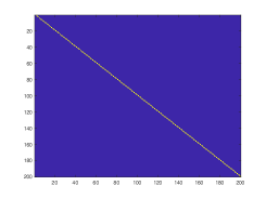
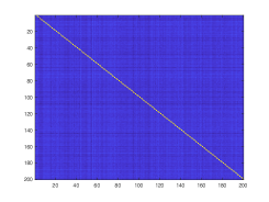
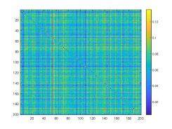
Figure 1: Comparison between GFIM and EFIM. Left: the GFIM, Middle: the 1st diagonal block of EFIM, Right: the difference between them.

2.3 Constructions of the Curvature Matrices

The curvature matrices can be constructed in other ways. We accumulate the statistics by momentum or use the mini-batch gradients. For simplicity, we do not write the multi-step strategy explicitly here.

Accumulate Statistics of Matrix by Momentum

Alternatively, we can replace the subsampled matrices (4) and (5) by:

$$\overline{L}_{k} =\beta\overline{L}_{k-1}+(1-\beta)L_{k},$$ (11)

$$\overline{R}_{k} =\beta\overline{R}_{k-1}+(1-\beta)R_{k},$$

where $\overline{L}_{0}=L_{0}$, $\overline{R}_{0}=R_{0}$ and $\beta$ is the momentum parameter.

Construct Matrix by Mini-Batch Gradients

At each iteration, the mini-batch gradient $\mathcal{G}_{B_{k}}$ is used to update the curvature matrices $\widetilde{L}_{k}$ and $\widetilde{R}_{k}$:

$$\widetilde{L}_{k} =\beta\widetilde{L}_{k-1}+\gamma\mathcal{G}_{B_{k}}\mathcal{G}_{B_{k}}^{\top},$$ (12)

$$\widetilde{R}_{k} =\beta\widetilde{R}_{k-1}+\gamma\mathcal{G}_{B_{k}}^{\top}\mathcal{G}_{B_{k}},$$

where $\widetilde{L}_{0}=\lambda_{0}I$, $\widetilde{R}_{0}=\lambda_{0}I$, $\beta$ and $\gamma$ are the parameters for momentum. The mechanism reuses the mini-batch gradients and can be regarded as an online update of GFIM.

2.4 Comparisons with Related Works

The most related approaches are KFAC and Shampoo. To make the difference clearer, we take a fully-connected layer ($m<n$) as an example. Given a sample set $S_{k}$, the directions of three methods are listed as below:

$$D_{k}=\left\{\begin{array}[]{ll}-(\lambda_{k}I+L_{k})^{-1}\mathbf{G}_{k},&\text{NG+},\vspace{1ex}\\ -(\widehat{L}_{k})^{-1/4}\mathbf{G}_{k}(\widehat{R}_{k})^{-1/4},&\text{Shampoo},\vspace{1ex}\\ -(\widetilde{A}_{k})^{-1}\mathbf{G}_{k}(\widetilde{G}_{k})^{-1},&\text{KFAC},\vspace{1ex}\\ \end{array}\right.$$ (13)

where $\widetilde{G}_{k}=\sqrt{\lambda_{k}}I+\frac{1}{|S_{k}|}\sum_{i\in S_{k}}g_{i}g_{i}^{\top}$ and $\widetilde{A}_{k}=\sqrt{\lambda_{k}}I+\frac{1}{|S_{k}|}\sum_{i\in S_{k}}a_{i}a_{i}^{\top}$. $\widehat{L}_{k}$ and $\widehat{R}_{k}$ in Shampoo are exactly $\widetilde{L}_{k}$ and $\widetilde{R}_{k}$ in (12) by choosing $\beta=\gamma=1$.

Assume that the matrix update frequency of all three methods are the same. NG+ needs to compute the inverse of $L_{k}$ and a matrix-matrix multiplication. The computational cost of KFAC is more than twice that of our method. Shampoo needs to update two matrices and obtain the -1/4 inverse of both two matrices whose computational cost is much more than that of computing the inverse. Although a coupled Newton method is used in [2], the implementation is more complicated and the end-users need to tune more hyper parameters.

In the distributed setting, KFAC has to synchronize two matrices with the size $m^{2}$ and $n^{2}$ while NG+ usually needs to synchronize $L_{k}$ whose size $\min\{m^{2},n^{2}\}$ is smaller. When the matrix of NG+ is chosen by (12), we do not need synchronize $L_{k}$ explicitly. KFAC and Shampoo store two different matrices and the storage is $m^{2}+n^{2}$. However, NG+ only stores one matrix and the storage is $\min\{m^{2},n^{2}\}$. This means the extra memory overhead of NG+ is smaller than the memory overhead of storing a tensor with the same size as gradient. It leads to an advantage in certain cases, for example, when one of the dimensions of embedding matrix may be 10 million or even more.

2.5 Computational Complexity

We next show the detailed extra computational operations compared with SGD. At each iteration, the construction of $L_{k}$, the inversion $L_{k}^{-1}$, and a matrix multiplication of $L_{k}^{-1}\mathbf{G}_{k}$ need to be computed. The computational cost of the first two operations can be controlled by the multi-step strategy. The last matrix multiplication is embarrassingly fast in GPUs. Note that in practice, we can simply let the sample set $S_{k}=B_{k}$ when constructing $L_{k}$.

The computation of $L_{k}$ for the cases (11) and (12) is a little bit different. For the case (11), we need to use the gradients of each sample. Note that commonly the deep learning framework such as PyTorch yields mini-batch gradient. Luckily, the required information $\{G_{i},A_{i}\}$ are already computed and can be stored in the process of computing the mini-batch gradient. In distributed cases with $\mathcal{M}$ devices, the sample set is split by $S_{k}=[S_{k,1},\dots,S_{k,\mathcal{M}}]$. We compute matrix $L_{k,j}=\frac{1}{|S_{k,j}|}\sum_{i\in S_{k,j}}\mathcal{G}_{i,k}\mathcal{G}_{i,k}^{\top}$ with sample slices $S_{k,j}$ and then average (All-Reduce) them among all devices. The synchronous cost can be also controlled by the delayed update strategy. Since the case (12) uses the mini-batch gradient, we do not need extra distributed communication operations.

3 Efficient Computation of the GFIM Direction

3.1 Utilize the Structure of the Gradients

In this part, we show how to save computational cost by taking full use of the structures of the gradients. Take the case $m\leq n$ as an example. In neural networks, the gradient is computed by back propagation (BP) process and often has the format (8) where $G_{i}$ and $A_{i}$ are obtained from backward and forward processes, respectively. Specifically, $\kappa$ in fully-connected layers and embedding layers equals 1 while $\kappa$ in convolutional layer is larger. Unluckily, $m$ and $n$ can be both very huge in applications. Hence, the cost of computing the inversion might be expensive.

When $\kappa$ =1, $g_{i,k}$ and $a_{i,k}$ are actually vectors and $L_{k}$ degenerates to be $\lambda_{k}I$ plus a low-rank matrix:

$$L_{k}=\lambda_{k}I_{m\times m}+\frac{1}{|B_{k}|}\sum_{i\in B_{k}}c_{i,k}g_{i,k}g_{i,k}^{\top},$$

where $c_{i,k}=a_{i,k}^{\top}a_{i,k}$ is a scalar. By using the Sherman-Morrison-Woodbury (SMW) formula, we obtain:

$$L_{k}^{-1}=\frac{1}{\lambda_{k}}I-{U_{k}}\left(\lambda_{k}I+{U_{k}}^{\top}U_{k}\right)^{-1}U_{k}^{\top},$$ (14)

where ${U_{k}}=\frac{1}{\sqrt{|B_{k}^{{}^{\prime}}|}}\left[\sqrt{c_{1,k}}g_{1,k},\dots,\sqrt{c_{|B_{k}^{{}^{\prime}}|,k}}g_{|B_{k}^{{}^{\prime}}|,k}\right]\in\mathbb{R}^{m\times|B_{k}^{{}^{\prime}}|}.$ It is already shown in [28] that computing $(\lambda_{k}I+L_{k})^{-1}\mathbf{G}_{k}$ by (14) is equivalent to a regularized least squares (LS) problems as follows:

$$\min_{D\in\mathbb{R}^{m\times n}}\|U_{k}D-\mathbf{G}_{k}\|_{F}^{2}+\lambda\|D\|_{F}^{2}.$$ (15)

To reduce the computational complexity, we can instead solve the following sketching LS problems:

$$\min_{D\in\mathbb{R}^{m\times n}}\|\Omega_{k}U_{k}D-\Omega_{k}\mathbf{G}_{k}\|_{F}^{2}+\lambda\|D\|_{F}^{2},$$ (16)

where $\Omega_{k}\in\mathbb{R}^{q\times m},q\ll m$ is a sketching matrix.

However, when $\kappa\neq$1, the summation part of $L_{k}$ is usually not a low-rank matrix and it is not reasonable to use SMW to reduce the computational complexity. Instead, we consider the following two strategies. Note that these strategies also work when $\kappa=1$.

3.2 Matrix Multiplications by Sketching

The computational complexity of $\mathcal{G}_{k}^{\top}\mathcal{G}_{k}$ or $\mathcal{G}_{k}\mathcal{G}_{k}^{\top}$ is still not tractable when both $m$ and $n$ are very huge. Here, we take sketching techniques to reduce the complexity. Similar idea is already used in the Newton Sketch method [19]. Given a sketching matrix $\Omega_{k}\in\mathbb{R}^{n\times q}$ where $E[\Omega_{k}\Omega_{k}^{\top}]=I_{n}$ and $q\ll n$, the matrix $\mathcal{G}_{k}\mathcal{G}_{k}^{\top}$ can be approximated by

$$\mathcal{G}_{k}\mathcal{G}_{k}^{\top}\approx\left(\mathcal{G}_{k}\Omega_{k}\right)\left(\mathcal{G}_{k}\Omega_{k}\right)^{\top}.$$

Here, we consider random uniform row samplings. Specifically, each column of $\Omega_{:,i},\;i=1,2,\dots,q,$ is sampled from

$$\omega\leftarrow\sqrt{\frac{n}{q}}e_{i},i=1,2,\dots,n,$$ (17)

with probability $\frac{1}{n}$, where $e_{i}\in\mathbb{R}^{n}$ is the vector whose $i$-th element is 1 and 0 otherwise. Note that sketching the matrix $\mathcal{G}_{k}$ by uniform row sampling does not involve extra computation and can be finished easily. There are also other different sketchy ways.

3.3 Block-Diagonal Approximation to the Curvature Matrix

We can use a diagonal matrix to approximate $L_{k}$ or $R_{k}$. Assume that $m=sp$ and denote $(\mathcal{G}_{k})_{(i-1)p+1:ip,:}$ by $\mathcal{G}_{k}^{i,p}$, where $i=1,2,\dots,s$. The approximation is presented as follows:

$$\mathcal{G}_{k}\mathcal{G}_{k}^{\top}\approx\operatorname{diag}\{\mathcal{G}_{k}^{1,p}(\mathcal{G}_{k}^{1,p})^{\top},\dots,\mathcal{G}_{k}^{s,p}(\mathcal{G}_{k}^{s,p})^{\top}\}.$$ (18)

Since the size of each $\mathcal{G}_{k}^{i,p}(\mathcal{G}_{k}^{i,p})^{\top}$ is the same, computing the inverse of $\mathcal{G}_{k}^{i,p}(\mathcal{G}_{k}^{i,p})^{\top}$ can be done in a batched fashion, which is significantly faster than inverting each matrix individually. By using (18), the computational cost reduces from $O(m^{3})$ to $O(sp^{3})$.

4 Theoretical Analysis

4.1 Global Convergence

In this part, the convergence analysis of NG+ is established. We make the following standard assumptions in stochastic optimization. Assume that $m\leq n$ and $\mathcal{T}$ is a constant just for simplicity.

Assumption 1.

We assume that $\Psi(\cdot)$ satisfies the following conditions.

1. $\Psi(\Theta)$ is continuous differentiable on $\mathbb{R}^{m\times n}$ and has a lower bound, i.e., $\Psi(\Theta)\geq\Psi^{*}$ for any $\Theta$. The gradient $\nabla\Psi(\Theta)$ is ${L}_{\Psi}$-Lipschitz continuous, i.e. $\|\nabla\Psi(\Theta_{1})-\nabla\Psi(\Theta_{2})\|_{F}\leq{L}_{\Psi}\|\Theta_{1}-\Theta_{2}\|_{F}.$

2. There exists positive constants $h_{1}$, $h_{2}$ such that $h_{1}I\preceq L_{k}+\lambda_{k}I\preceq h_{2}I$ holds for all $k$.

3. The mini-batch gradient is unbiased a.s. $\nabla\Psi(\Theta_{k})=\mathbb{E}[G_{k}|\Theta_{k},\cdots,\Theta_{0}]$ and has bounded variance $\mathbb{E}[\|G_{k}-\nabla\Psi(\Theta_{k})\|_{F}^{2}|\Theta_{k},\cdots,\Theta_{0}]\leq\sigma_{k}^{2}$ for all $k$.

These assumptions are broadly used in second-order methods, such as [27, 7]. We now present the global convergence guarantee of NG+.

Theorem 2.

Suppose that Assumption 1 is satisfied and the step size $\{\alpha_{k}\}$ satisfies $\alpha_{k}\leq\frac{2h_{1}^{2}}{L_{\Psi}h_{2}}$, $\sum\alpha_{k}=\infty$ and $\sum\alpha_{k}^{2}\sigma_{k}^{2}<\infty$. Then with probability 1 we have

$$\lim_{k\rightarrow\infty}\|\nabla\Psi(\Theta_{k})\|_{F}=0.$$

We next consider the complexity of NG+ and the following theorem implies that $O(\epsilon^{-\frac{1}{\beta}})$ iterations are enough to guarantee that $\frac{1}{\hat{T}}\sum_{k=1}^{\hat{T}}\mathbb{E}[\|\Psi(\Theta_{k})\|^{2}]\leq\epsilon$.

Theorem 3.

Suppose that Assumption 1 is satisfied and the step size is chosen as $\alpha_{k}=\frac{2h_{1}^{2}}{L_{\Psi}h_{2}}k^{-\beta},$ where $\beta\in(0.5,1)$ and $\sigma_{k}\equiv\sigma$ for all $k$. Then we have

$$\frac{1}{\hat{T}}\sum_{k=1}^{\hat{T}}\mathbb{E}[\|\Psi(\Theta_{k})\|^{2}]\leq\frac{L_{\Psi}h_{2}^{2}}{h_{1}^{2}}\hat{T}^{-1}+\frac{2\sigma^{2}}{h_{2}^{2}(1-\beta)}\hat{T}^{-\beta},$$

where $\hat{T}$ is the number of iterations.

The proof of the above two theorems can be found in the Appendix.

4.2 Regret Analysis

In this part, we consider the regret bound of one variant of NG+ under standard online convex optimization setting. The regret is defined as follows:

$$\mathcal{R}_{T}=\sum_{t=1}^{T}\psi_{t}(\Theta_{t})-\inf_{\Theta^{*}\in\mathcal{K}}\left(\sum_{t=1}^{T}\psi_{t}(\Theta^{*})\right),$$

where $\psi_{t}:\mathcal{K}\rightarrow\mathbb{R}$ is a convex cost function, $\Theta_{t}\in\mathcal{K}$ and $\mathcal{K}$ is a bounded convex set, i.e., $\forall X,Y\in\mathcal{K}$, we have $\|X-Y\|_{F}\leq\mathcal{D}$. We analyze the following iteration process which can be regarded as an extension of the online Newton method [9]:

$$L_{t}=L_{t-1}+\nabla\psi_{t}^{\top}\nabla\psi_{t},\quad\Theta_{t+1}=\Pi_{\mathcal{K}}(\Theta_{t}-\frac{1}{\alpha}L_{t}^{-1}G_{t}),$$ (19)

where $L_{0}=\epsilon I$, $\alpha$ is the step size. A few necessary assumptions are listed below.

Assumption 4.

We assume each $\psi_{t}(\cdot)$ satisfies the following conditions:

1. For any $t=1,2,\cdots$, the function $\psi_{t}$ satisfies: $\psi_{t}(X)\geq\psi_{t}(Y)+\langle\nabla\psi_{t}(Y),X-Y\rangle+\frac{\alpha}{2}\|X-Y\|_{\nabla\psi_{t}(Y)\nabla\psi_{t}(Y)^{\top}}^{2},$ for $X,Y\in\mathcal{K},$ where $\|X-Y\|_{\nabla\psi_{t}(Y)\nabla\psi_{t}(Y)^{\top}}^{2}=\mathrm{Tr}\left((X-Y)^{\top}\nabla\psi_{t}(Y)\nabla\psi_{t}(Y)^{\top}(X-Y)\right).$

2. The norm of the gradient $\nabla\psi_{t}$ is bounded by $\mathcal{L}_{G}$, i.e., $\|\nabla\psi_{t}\|_{F}\leq\mathcal{L}_{G}$.

When $n=1$, the function satisfying Assumption 4.1 is actually the $\alpha$-exp-concave function [hazan2007logarithmic]. We summarize our logarithmic regret bound as follows.

Theorem 5.

Let $\epsilon=\frac{2}{\alpha\mathcal{D}^{2}}$. If Assumption 4 is satisfied, then the regret $\mathcal{R}_{T}$ can be bounded by

$$\mathcal{R}_{T}\leq\frac{n}{\alpha}\log\alpha\mathcal{L}_{G}^{2}\mathcal{D}^{2}T.$$

The proof is shown in the Appendix.

5 Numerical Experiments

5.1 Image Classification

The training of ResNet50 [10] on ImageNet-1k [5] dataset is one of the basic experiments in image classification [15]. We compare NG+ with LARS [30], SGD with momentum (SGD for short) and KFAC. The experiments of LARS are based on the implementation and tuned in the same way as Table 3 in [31]. SGD is taken from the default version in PyTorch. The result of ADAM is not reported because it does not perform well in ResNet50 with ImageNet-1k task. We do not report the results of Shampoo since an efficient implementation of Shampoo in PyTorch is not officially available and our current codes do not take advantage training on heterogeneous hardwares. We follow the standard settings and use the same basic dataset augmentation as the official PyTorch example without changing the figure sizes throughout the training process. The training process of all methods are terminated once the top-1 testing accuracy equals or exceeds 75.9%. All codes are written in PyTorch and available in https://github.com/yangorwell/NGPlus.

Table 1: Detailed Statistics on image classification when top-1 testing accuracy achieves 75.9%.

	# Epoch	Total Time	Time Per Epoch
SGD	76	10.9 h	517 s
LARS	74	10.7 h	521 s
KFAC	42	8.0 h	686 s
NG+	40	6.7 h	600 s

We first consider a batch size $256$. Note that the SGD achieves top-1 testing accuracy 75.9% within 76 epochs, which is well tuned. The changes of testing accuracy and training accuracy versus training time are reported in Figure 2 and detailed statistics are shown in Table 1. We can see that NG+ performs best in the total training time and only takes 40 epochs to reach 75.9% top-1 testing accuracy. Compared with SGD and LARS, NG+ has at least 45% and 37% reduction in the number of epochs and training time, respectively. Although NG+ is better than KFAC for only two epochs, it leads to 16% reduction in terms of the computing time.

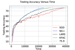
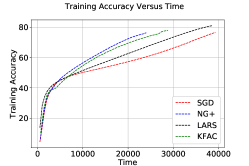
Figure 2: Numerical performance on ResNet50 on ImageNet-1k.

Figure 3: Numerical performance of SchNet on QM9 and MatProj.

(a) QM9: Loss VS Time.

(b) QM9: Loss VS Epoch.

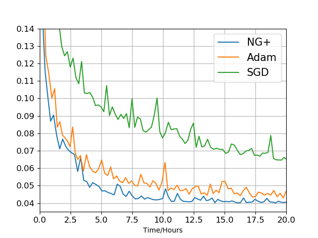
(c) MatProj: Loss VS Time.

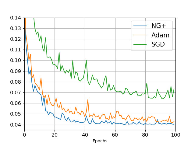
(d) MatProj: Loss VS Epoch.

We further consider the large-batch training. Since our GPUs are limited, we accumulate mini-batch gradients sampled in several steps to obtain the gradient of a larger batch. Hence, only the statistics on the epochs and iterations are reported and can be found in Table 2. The number of epochs for the batch sizes 2048 and 4096 is 41. By running more experiments and finding more reliable tuning strategies, it is expected that the number of epochs can be further reduced for the large-batch setting.

Table 2: Detailed Statistics of NG+ on ImageNet-1k for different Batch Sizes.

# Batch Size	256	2048	4096
# Epoch	40	41	41
#Iteration	200k	25.6k	12.8k

5.2 Quantum Chemistry

Deep learning has been applied to quantum chemistry problems. SchNet is a well-known network architecture in quantum chemistry modeling [24]. We compare NG+ with SGD and Adam [13] by using SchNetPack on the benchmark datasets QM9 [20] and Materials Project (MatProj) [11]. The numerical results are presented in Figure 4(d) where we can see the validation loss of NG+ is much better than Adam in terms of both iteration and time on QM9 and MatProj datasets. For example, on MatProj, when the validation loss attains 0.05, NG+ needs less than 20 epochs and spends about 4 hours. On the other hand, Adam needs more than 30 epochs and consumes about 7.5 hours.

5.3 Neural Machine Translation

We consider the neural machine translation task in this part. The implementation is based on the fairseq [17] and we use default transformer “iwslt_de_en_v2” architecture therein. The IWSLT14 [4] German-to-English dataset is used. We present the training loss and validation loss through the training process in Figure 4. In the training set, the training loss curve of NG+ is always below that of Adam. We also report the BLEU score in the testing set. The result (mean and standard deviation) over 3 independent runs of NG+ is $34.79\pm 0.09$ while the BLEU score of Adam is $34.75\pm 0.08$.

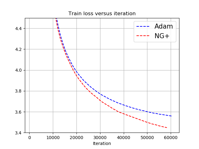
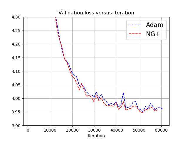
Figure 4: Numerical performance on IWSLT14 (Transformer).

5.4 Recommendation System

We test the performance of NG+ on the recommendation models DLRM [16] which is widely considered in industry. The Criteo Ad Kaggle dataset in this part contains nearly 45 million samples in one week. The data points of the first six days are used for training set while the others are used for testing set. We train the model for one epoch, compare NG+ with SGD, AdaGrad [6] and report the Click Through Rate (CTR) on the training and testing set in Figure 5. The best testing accuracy of AdaGrad is 79.149% while that of NG+ is 79.175%. Our proposed method has at least 0.025% higher testing accuracy which is a good progress in this topic [26].

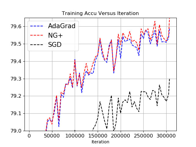
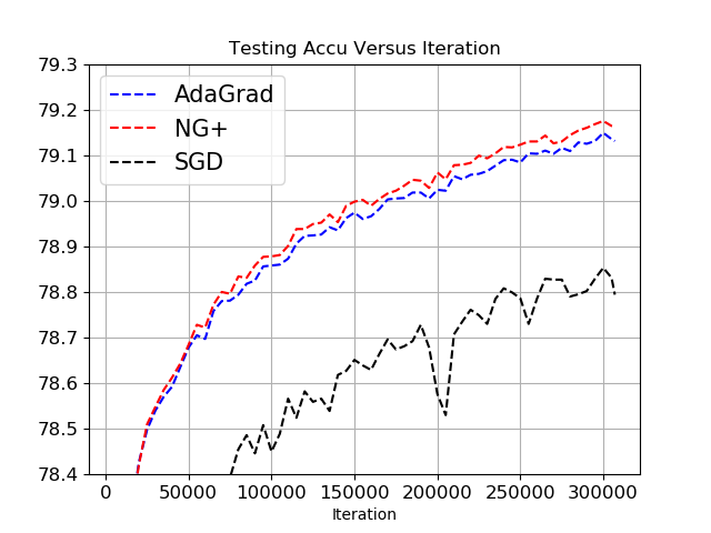
Figure 5: Numerical performance on DLRM model.

6 Conclusion

In this paper, we propose a multi-step matrix-product natural gradient method NG+. It is based on an intuitive extension of the Fisher information matrix to the matrix space. The size of the coefficient matrix to be inverted is reasonably small and the computational cost is reduced comparing to the state-of-the-art methods including KFAC and Shampoo. The global convergence property is analyzed under some mild conditions and a regret bound is given in the online convex optimization case. Numerical experiments on important tasks, such as image classification with ResNet50, quantum chemistry modeling with Schnet, neural translation with Transformer and recommendation system with DLRM, show that NG+ is quite promising.

The performance of NG+ can be further improved in several aspects, including accelerating the training process and improving the testing accuracy, with the help of a number of techniques such as sketching, more reliable learning rates strategies and training on heterogeneous hardware. Implementing the fundamental operations such as the computing of sample gradients and matrix inversion in a more efficient and friendly way is also critical to second-order type methods. A few particularly important topics of investigation are (i) a comprehensive study of the issue of larger batch sizes, (ii) a careful design for the parallel efficiency, and (iii) extensive experiments on various large learning tasks.

Appendix A Implementation Details

In this section, we describe the implementation details of the numerical experiments.

• ResNet50 on ImageNet-1k:

  • We first consider the case where the batch size is 256. We use the official implementation of ResNet50 (also known as ResNet50 v1.5) in PyTorch. The detailed network structures can be found in the website: https://pytorch.org/docs/stable/_modules/torchvision/models/resnet.html. We use the linear warmup strategy [8] in the first 5 epochs for SGD, KFAC and NG+.

    • SGD uses the cosine learning rate strategy

      $$\alpha_{k}=0.001+0.5*(\alpha_{0}-0.001)*(1+\text{cos(epoch\_k / max\_epoch}*\pi))$$

      for given parameters max_epoch and the initial learning rate $\alpha_{0}$. The hyper-parameters are the same as those on the website and the result reported here achieves top-1 testing accuracy 75.9% within 76 epochs. This is better than the result of using the diminishing learning rate strategy in official PyTorch example, which needs nearly 90 epochs.

    • LARS uses the codes from the website and we use the recommended parameters from [31].

    • KFAC uses the exponential strategy

      $$\alpha_{k}=\alpha_{0}*(1-\text{epoch\_k/max\_epoch)}^{\mathcal{\widetilde{D}}},$$

      for given the max_epoch, decay rate $\mathcal{\widetilde{D}}$ and the initial learning rate $\alpha_{0}$. The max_epoch is set to be 60. The initial learning rate is from {0.05, 0.1, 0.15} and initial damping $\lambda_{0}$ is from {0.05, 0.1, 0.15} and we report the best results among them. The damping is set to be $\lambda_{0}\cdot(0.87)^{\text{epoch\_k}/10}$. The update frequency which means $\mathcal{T}$ in multi-step strategy is 500.

    • NG+ uses the exponential strategy by letting max_epoch to be 52, the initial learning rate to be 0.18 and decay_rate to be 5, respectively. The damping parameter $\lambda_{k}$ is set to be 0.16$\cdot(0.8)^{\text{epoch\_k}/10}$. The update frequency is 500.

  • For large-batch training, the detailed hyper-parameters for each batch-size are listed in Table 3.

    Batch Size	$\alpha_{\text{warmup}}$	warm-up epoch	$\alpha_{0}$	decay_rate	max_epoch	damping $\lambda$
    2, 048	0.01	5	1.3	5	50	0.2$\cdot(0.7)^{(\text{epoch\_k}/10)}$
    4, 096	0.01	5	2.6	5	50	0.3$\cdot(0.7)^{(\text{epoch\_k}/10)}$

    Table 3: Detailed hyper-parameters for different batch sizes.

• SchNet:

  We use SchNetPack and implement our proposed NG+ within this package. The weight decay is set to be 1e-5 for all the experiments. To train the model efficiently, it is highly recommended to put all the datasets on an Solid State Disk(SSD).

  • For NG+, we use the learning rate schedule $\alpha_{k}=\text{2e-4}\cdot\text{max}(\text{epoch\_k}-10,1)^{-0.5}$. Damping is 0.17 for QM9, 0.6 for MatProj. The update frequency is set to 200.

  • For Adam, we grid search the learning rate from 1e-5, 2e-5, 4e-5, 1e-4, 2e-4, 4e-4 and choose 1e-4 for both MatProj and QM9. We also consider the schedule used in NG+ but it does not perform well in Adam.

  • For SGD, we set the learning rate 4e-4 for QM9, 5e-3 for MatProj.

• Transformer:

  We use the fairseq and implement our proposed NG+ within this package. The batch size and the weight decay is set to be 4096 and 1e-4, respectively.

  • For Adam, we set the initial learning rate to be 5e-4, eps to be 1e-8, $\beta_{1}$ to be $0.9$, $\beta_{2}$ to be $0.98$, the number of warmup-updates to be 10000 and the learning rate scheduler to be inverse_sqrt, which is similar to the recommended example .

  • For NG+, the initial learning rate is set to be 6e-4 and the damping is set to be $0.3\cdot 0.87^{(\text{epoch\_k}/10)}$. Other parameters are the same as Adam.

• DLRM:

  We use the code in the website and change the optimizer to our proposed NG+. None of the optimizer applies the weight decay.

  • For NG+, we set the learning rate 0.015, damping 1.0 and the update frequency 1000.

  • For Adagrad, we set the learning rate 0.01.

  • For SGD, we set the learning rate 0.1, with all other parameters identical to the file.

Appendix B Proof of Theorem 2

Proof.

We define $\mathbb{E}_{k}[\cdot]=\mathbb{E}[\cdot|\Theta_{k},\cdots,\Theta_{0}]$. By Assumption 1, it holds:

$$\mathbb{E}_{k}[\Psi(\Theta_{k+1})] \leq\mathbb{E}_{k}\left[\Psi(\Theta_{k})+\langle\nabla\Psi(\Theta_{k}),\Theta_{k+1}-\Theta_{k}\rangle+\frac{L_{\Psi}}{2}\|\Theta_{k+1}-\Theta_{k}\|_{F}^{2}\right]$$ (20)

$$=\Psi(\Theta_{k})+\mathbb{E}_{k}\left[\langle\nabla\Psi(\Theta_{k}),-\alpha_{k}L_{k}^{-1}G_{k}\rangle\right]+\mathbb{E}_{k}\left[\frac{L_{\Psi}\alpha_{k}^{2}}{2}\|L_{k}^{-1}G_{k}\|_{F}^{2}\right]$$

$$\leq\Psi(\Theta_{k})+\langle\nabla\Psi(\Theta_{k}),-\alpha_{k}L_{k}^{-1}\nabla\Psi(\Theta_{k})\rangle+\frac{L_{\Psi}\alpha_{k}^{2}}{2h_{1}^{2}}\mathbb{E}_{k}\left[\|G_{k}\|_{F}^{2}\right]$$

$$\leq\Psi(\Theta_{k})-\frac{\alpha_{k}}{h_{2}}\|\nabla\Psi(\Theta_{k})\|_{F}^{2}+\frac{L_{\Psi}\alpha_{k}^{2}}{2h_{1}^{2}}\left(\|\nabla\Psi(\Theta_{k})\|_{F}^{2}+\sigma_{k}^{2}\right)$$

$$\leq\Psi(\Theta_{k})-\left(\frac{\alpha_{k}}{h_{2}}-\frac{L_{\Psi}\alpha_{k}^{2}}{2h_{1}^{2}}\right)\|\nabla\Psi(\Theta_{k})\|_{F}^{2}+\frac{L_{\Psi}\alpha_{k}^{2}}{2h_{1}^{2}}\sigma_{k}^{2}.$$

Using $\alpha_{k}\leq\frac{2h_{1}^{2}}{L_{\Psi}h_{2}}$, summing over above inequality from $0$ to $\infty$, and taking the expectation yield

$$\sum_{k=0}^{\infty}\frac{\alpha_{k}}{2h_{2}}\mathbb{E}\|\nabla\Psi(\Theta_{k})\|_{F}^{2}\leq\Psi(\Theta_{0})-\Psi^{*}+\frac{L_{\Psi}}{2h_{1}^{2}}\sum_{k=0}^{\infty}\alpha_{k}^{2}\sigma_{k}^{2}<\infty.$$

Since $\sum_{k=0}^{\infty}\alpha_{k}=\infty$, we have $\liminf_{k\rightarrow\infty}\|\nabla\Psi(\Theta_{k})\|_{F}=0$ with probability 1.

We next prove $\lim_{k\rightarrow\infty}\|\nabla\Psi(\Theta_{k})\|_{F}=0$ by contradiction. Suppose that there exists $\epsilon>0$ and two increasing sequences $\{a_{i}\}_{i=1}^{\infty}$ and $\{b_{i}\}_{i=1}^{\infty}$ such that $a_{i}<b_{i}$ and

$$\left\{\begin{aligned} \|\nabla\Psi(\Theta_{k})\|\geq 2\epsilon,&&k=a_{i},\\ \|\nabla\Psi(\Theta_{k})\|\geq\epsilon,&&a_{i}<k<b_{i},\\ \|\nabla\Psi(\Theta_{k})\|\leq\epsilon,&&k=b_{i}.\end{aligned}\right.$$

Hence, it follows that

$$\epsilon^{2}\sum_{i=1}^{\infty}\sum_{k=a_{i}}^{b_{i}-1}\alpha_{k}\leq\sum_{i=1}^{\infty}\sum_{k=a_{i}}^{b_{i}-1}\alpha_{k}\|\nabla\Psi(\Theta_{k})\|^{2}\leq\sum_{k=1}^{\infty}\alpha_{k}\|\nabla\Psi(\Theta_{k})\|^{2}\leq\infty,$$

which implies $\lim_{i\rightarrow\infty}\sum_{k=a_{i}}^{b_{i}-1}\alpha_{k}=0$.

In addition, we have

$$\mathbb{E}\left[\sum_{k=a_{i}}^{b_{i}-1}\alpha_{k}^{-1}\|\Theta_{k+1}-\Theta_{k}\|_{2}^{2}\right] =\mathbb{E}\left[\sum_{k=a_{i}}^{b_{i}-1}\alpha_{k}\|L_{k}^{-1}G_{k}\|_{2}^{2}\right]\leq\mathbb{E}\left[\sum_{k=a_{i}}^{b_{i}-1}\frac{\alpha_{k}}{h_{1}^{2}}\left(\|\nabla\Psi(\Theta_{k})\|_{2}^{2}+\sigma_{k}^{2}\right)\right]<\infty.$$

By Hölder inequality, we obtain

$$\|\Theta_{a_{i}}-\Theta_{b_{i}}\|_{2}^{2}\leq\left(\sum_{k=a_{i}}^{b_{i}-1}\alpha_{k}\right)\left(\sum_{k=a_{i}}^{b_{i}-1}\alpha_{k}^{-1}\|\Theta_{k+1}-\Theta_{k}\|_{2}^{2}\right),$$

which implies $\lim_{i\rightarrow\infty}\|\Theta_{a_{i}}-\Theta_{b_{i}}\|_{2}^{2}=0$. However, we have $\|\nabla\Psi(\Theta_{a_{i}})-\nabla\Psi(\Theta_{b_{i}})\|_{2}\geq\epsilon$, which is a contradiction by the Lipschitz-continuous property of $\nabla\Psi(\Theta)$. This finishes the proof. ∎

Appendix C Proof of Theorem 3

Proof.

From (20), we have

$$\|\nabla\Psi(\Theta_{k})\|^{2}\leq\frac{2h_{2}}{\alpha_{k}}\Psi(\Theta_{k})-\frac{2h_{2}}{\alpha_{k}}\mathbb{E}_{k}[\Psi(\Theta_{k+1})]+\frac{L_{\Psi}\alpha_{k}}{h_{1}^{2}h_{2}}\sigma^{2}.$$

Taking expectation and summing over $k$ from $1$ to $N$, we obtain

$$\sum_{k=1}^{N}\mathbb{E}[\|\nabla\Psi(\Theta_{k})\|^{2}] \leq\frac{2h_{2}}{\alpha_{1}}\mathbb{E}\Psi(\Theta_{1})+\sum_{k=2}^{N}(\frac{2h_{2}}{\alpha_{k}}-\frac{2h_{2}}{\alpha_{k-1}})\mathbb{E}\Psi(\Theta_{k})+\sum_{k=1}^{N}\frac{L_{\Psi}\alpha_{k}}{h_{1}^{2}h_{2}}\sigma^{2}$$

$$\leq\frac{2h_{2}}{\alpha_{1}}M+\sum_{k=1}^{N}\frac{L_{\Psi}\sigma^{2}}{h_{1}^{2}h_{2}}\alpha_{k}$$

$$\leq\frac{L_{\Psi}h_{2}^{2}}{h_{1}^{2}}+\frac{2\sigma^{2}}{h_{2}^{2}(1-\beta)}(N^{1-\beta}-1),$$

which proves the theorem. ∎

Appendix D Proof of Theorem 5

We first give an example that satisfies the Assumption 4.1.

Example Suppose that $\|X\|\leq 1$, $\|Y\|_{2}\leq R$ and $\mathcal{K}=\{W\in\mathbb{R}^{m\times n}|\|W\|_{2}\leq R\}$ for a given value $R$, then $f(W)=\frac{1}{2}\|W^{\top}X-Y\|_{2}^{2}$ satisfies Assumption 4.1.

Proof.

With a slight abuse of the notation, we define $f(\text{vec}(W))=f(W)$. We have $\nabla f(W)=XX^{\top}W-XY^{\top}$ and $\nabla^{2}f(\text{vec}(W))=I\otimes XX^{\top}$. To show that $f(W)$ satisfies Assumption 4.1, we only need to prove that there exists a $\alpha$ such that for all $W$, we have $\nabla^{2}f(\text{vec}(W))\succeq\alpha I\otimes\nabla f(W)\nabla f(W)^{\top}$.

$$\nabla f(W)\nabla f(W)^{\top} =X(X^{\top}W-Y^{\top})(X^{\top}W-Y^{\top})^{\top}X^{\top}$$

$$\preceq X4R^{2}IX^{\top}$$

$$=4R^{2}XX^{\top}.$$

Thus for $\alpha=\frac{1}{4R^{2}}$, we have $\nabla^{2}f(\text{vec}(W))\succeq\alpha I\otimes\nabla f(W)\nabla f(W)^{\top}$. ∎

To prove Theorem 5, we give two required lemmas in the next.

Lemma 6.

Suppose that $\alpha\leq\alpha_{0}$ and Assumption 4 holds, then the regret can be bounded by

$$\mathcal{R}_{T}\leq\frac{1}{2\alpha}\sum_{t=1}^{T}\|G_{t}\|_{L_{t}^{-1}}^{2}+\frac{\alpha\epsilon\mathcal{D}^{2}}{2}.$$

Proof.

Let $\Theta^{*}\in\mathrm{argmin}_{\Theta\in\mathcal{K}}\sum_{t=1}^{T}\psi_{t}(\Theta)$ to be the minimizer in the hindsight. By Assumption 4, we have

$$\psi_{t}(\Theta_{t})-\psi_{t}(\Theta^{*})\leq\langle G_{t},\Theta_{t}-\Theta^{*}\rangle-\frac{\alpha}{2}\|\Theta^{*}-\Theta_{t}\|_{G_{t}G_{t}^{\top}}^{2}.$$

As $\Theta_{t+1}=\Pi_{\mathcal{K}}(\Theta_{t}-\frac{1}{\alpha}L_{t}^{-1}G_{t})$, we obtain

$$\|\Theta_{t+1}-\Theta^{*}\|_{L_{t}}^{2} \leq\|\Theta_{t}-\frac{1}{\alpha}L_{t}^{-1}G_{t}-\Theta^{*}\|_{L_{t}}^{2}$$

$$\leq\|\Theta_{t}-\Theta^{*}\|_{L_{t}}^{2}-\frac{2}{\alpha}\langle\Theta_{t}-\Theta^{*},G_{t}\rangle+\frac{1}{\alpha^{2}}\|G_{t}\|_{L_{t}^{-1}}^{2}.$$

Summing up over $t=1$ to $T$ yields

$$\sum_{t=1}^{T}\langle\Theta_{t}-\Theta^{*},G_{t}\rangle$$

$$= \frac{1}{2\alpha}\sum_{t=1}^{T}\|G_{t}\|_{L_{t}^{-1}}^{2}+\frac{\alpha}{2}\|\Theta_{1}-\Theta^{*}\|_{L_{0}}^{2}+\frac{\alpha}{2}\sum_{t=1}^{T}\|\Theta_{t}-\Theta^{*}\|_{L_{t}-L_{t-1}}^{2}-\frac{\alpha}{2}\|\Theta_{T+1}-\Theta^{*}\|_{L_{T}}^{2}$$

$$\leq \frac{1}{2\alpha}\sum_{t=1}^{T}\|G_{t}\|_{L_{t}^{-1}}^{2}+\frac{\alpha}{2}\epsilon\mathcal{D}^{2}+\frac{\alpha}{2}\sum_{t=1}^{T}\|\Theta_{t}-\Theta^{*}\|_{G_{t}G_{t}^{\top}}^{2}.$$

Thus we have

$$\sum_{t=1}^{T}\psi_{t}(\Theta_{t})-\psi_{t}(\Theta^{*})\leq\sum_{t=1}^{T}\langle G_{t},\Theta_{t}-\Theta^{*}\rangle-\frac{\alpha}{2}\|\Theta^{*}-\Theta_{t}\|_{G_{t}G_{t}^{\top}}^{2}\leq\frac{1}{2\alpha}\sum_{t=1}^{T}\|G_{t}\|_{L_{t}^{-1}}^{2}+\frac{\alpha\epsilon\mathcal{D}^{2}}{2}.$$

∎

We next present the matrix-form elliptical potential lemma. The proof is similar to the proof in [9]. For completeness, we provide the proof here.

Lemma 7.

Suppose $L_{0}=\epsilon I$, $L_{t+1}=L_{t}+G_{t}G_{t}^{\top}$ and $\|G_{t}\|_{2}\leq\mathcal{L}_{G}$ for all $t$, we have

$$\sum_{t=1}^{T}\|G_{t}\|_{L_{t}^{-1}}^{2}\leq\log\frac{|L_{T}|}{|L_{0}|}\leq n\log\left(\frac{T\mathcal{L}_{G}^{2}+\epsilon}{\epsilon}\right).$$ (21)

Proof.

By the matrix inequality $\langle A-B,B\rangle\geq\log\frac{|A|}{|B|}$ for $A\succeq B\succeq 0$, we have

$$\sum_{t=1}^{T}\|G_{t}\|_{L_{t}^{-1}}^{2} =\sum_{t=1}^{T}\langle G_{t}G_{t}^{\top},L_{t}\rangle\leq\sum_{t=1}^{T}\langle L_{t}-L_{t-1},L_{t}\rangle\leq\sum_{t=1}^{T}\log\frac{|L_{t}|}{|L_{t-1}|}=\log\frac{|L_{T}|}{|L_{0}|}.$$

Since $L_{T}=\sum_{t=1}^{T}G_{t}G_{t}^{\top}+\epsilon I$ and $\|G_{t}\|_{2}\leq\mathcal{L}_{G}$, the largest eigenvalue of $L_{T}$ is at most $T\mathcal{L}_{G}^{2}+\epsilon$. This finishes the proof. ∎

Finally, we can prove the logarithmic regret of our proposed method by combining all the lemmas together and setting an appropriate regularization coefficient.

Proof.

By Lemma 6 and Lemma 7, we have

$$\mathcal{R}_{T} \leq\frac{1}{2\alpha}\sum_{t=1}^{T}\|G_{t}\|_{L_{t}^{-1}}^{2}+\frac{\alpha\epsilon\mathcal{D}^{2}}{2}\leq\frac{1}{2\alpha}n\log(\frac{T\mathcal{L}_{G}^{2}+\epsilon}{\epsilon})+\frac{\alpha\epsilon\mathcal{D}^{2}}{2}\leq\frac{n}{\alpha}\log\alpha\mathcal{L}_{G}^{2}\mathcal{D}^{2}T,$$

which completes our proof. ∎

References

- [1] Martin Abadi, Paul Barham, Jianmin Chen, Zhifeng Chen, Andy Davis, Jeffrey Dean, Matthieu Devin, Sanjay Ghemawat, Geoffrey Irving, Michael Isard, Manjunath Kudlur, Josh Levenberg, Rajat Monga, Sherry Moore, Derek G. Murray, Benoit Steiner, Paul Tucker, Vijay Vasudevan, Pete Warden, Martin Wicke, Yuan Yu, and Xiaoqiang Zheng. Tensorflow: A system for large-scale machine learning. In 12th USENIX Symposium on Operating Systems Design and Implementation (OSDI 16), pages 265–283, 2016.
- [2] Rohan Anil, Vineet Gupta, Tomer Koren, Kevin Regan, and Yoram Singer. Scalable second order optimization for deep learning. arXiv preprint arXiv:2002.09018, 2020.
- [3] Richard H Byrd, Samantha L Hansen, Jorge Nocedal, and Yoram Singer. A stochastic quasi-newton method for large-scale optimization. SIAM Journal on Optimization, 26(2):1008–1031, 2016.
- [4] Mauro Cettolo, Jan Niehues, Sebastian Stüker, Luisa Bentivogli, and Marcello Federico. Report on the 11th iwslt evaluation campaign, iwslt 2014. In Proceedings of the International Workshop on Spoken Language Translation, Hanoi, Vietnam, volume 57, 2014.
- [5] Jia Deng, Wei Dong, Richard Socher, Li-Jia Li, Kai Li, and Li Fei-Fei. Imagenet: A large-scale hierarchical image database. In 2009 IEEE conference on computer vision and pattern recognition, pages 248–255. Ieee, 2009.
- [6] John Duchi, Elad Hazan, and Yoram Singer. Adaptive subgradient methods for online learning and stochastic optimization. Journal of machine learning research, 12(7), 2011.
- [7] Donald Goldfarb, Yi Ren, and Achraf Bahamou. Practical quasi-newton methods for training deep neural networks. arXiv preprint arXiv:2006.08877, 2020.
- [8] Priya Goyal, Piotr Dollár, Ross Girshick, Pieter Noordhuis, Lukasz Wesolowski, Aapo Kyrola, Andrew Tulloch, Yangqing Jia, and Kaiming He. Accurate, large minibatch SGD: Training ImageNet in 1 hour. ArXiv:1706.02677, 2017.
- [9] Elad Hazan, Amit Agarwal, and Satyen Kale. Logarithmic regret algorithms for online convex optimization. Machine Learning, 69(2-3):169–192, 2007.
- [10] Kaiming He, Xiangyu Zhang, Shaoqing Ren, and Jian Sun. Deep residual learning for image recognition. In IEEE Conference on Computer Vision and Pattern Recognition, pages 770–778, 2016.
- [11] Anubhav Jain, Shyue Ping Ong, Geoffroy Hautier, Wei Chen, William Davidson Richards, Stephen Dacek, Shreyas Cholia, Dan Gunter, David Skinner, Gerbrand Ceder, and Kristin A. Persson. Commentary: The materials project: A materials genome approach to accelerating materials innovation. APL Materials, 1(1):011002, 2013.
- [12] Nitish Shirish Keskar, Dheevatsa Mudigere, Jorge Nocedal, Mikhail Smelyanskiy, and Ping Tak Peter Tang. On large-batch training for deep learning: Generalization gap and sharp minima. In 5th International Conference on Learning Representations, ICLR 2017, Toulon, France, April 24-26, 2017, Conference Track Proceedings. OpenReview.net, 2017.
- [13] Diederik P Kingma and Jimmy Ba. Adam: A method for stochastic optimization. arXiv preprint arXiv:1412.6980, 2014.
- [14] James Martens and Roger Grosse. Optimizing neural networks with kronecker-factored approximate curvature. In International conference on machine learning, pages 2408–2417, 2015.
- [15] Peter Mattson, Christine Cheng, Cody Coleman, Greg Diamos, Paulius Micikevicius, David Patterson, Hanlin Tang, Gu-Yeon Wei, Peter Bailis, Victor Bittorf, et al. Mlperf training benchmark. arXiv preprint arXiv:1910.01500, 2019.
- [16] Maxim Naumov, Dheevatsa Mudigere, Hao-Jun Michael Shi, Jianyu Huang, Narayanan Sundaraman, Jongsoo Park, Xiaodong Wang, Udit Gupta, Carole-Jean Wu, Alisson G Azzolini, et al. Deep learning recommendation model for personalization and recommendation systems. arXiv preprint arXiv:1906.00091, 2019.
- [17] Myle Ott, Sergey Edunov, Alexei Baevski, Angela Fan, Sam Gross, Nathan Ng, David Grangier, and Michael Auli. fairseq: A fast, extensible toolkit for sequence modeling. In Proceedings of NAACL-HLT 2019: Demonstrations, 2019.
- [18] Adam Paszke, Sam Gross, Francisco Massa, Adam Lerer, James Bradbury, Gregory Chanan, Trevor Killeen, Zeming Lin, Natalia Gimelshein, Luca Antiga, et al. Pytorch: An imperative style, high-performance deep learning library. arXiv preprint arXiv:1912.01703, 2019.
- [19] Mert Pilanci and Martin J Wainwright. Newton sketch: A near linear-time optimization algorithm with linear-quadratic convergence. SIAM Journal on Optimization, 27(1):205–245, 2017.
- [20] Raghunathan Ramakrishnan, Pavlo O Dral, Matthias Rupp, and O Anatole Von Lilienfeld. Quantum chemistry structures and properties of 134 kilo molecules. Scientific data, 1(1):1–7, 2014.
- [21] Yi Ren and Donald Goldfarb. Kronecker-factored quasi-newton methods for convolutional neural networks. arXiv preprint arXiv:2102.06737, 2021.
- [22] Herbert Robbins and Sutton Monro. A stochastic approximation method. Ann. Math. Stat., 22:400–407, 1951.
- [23] Farbod Roosta-Khorasani and Michael W Mahoney. Sub-sampled newton methods. Mathematical Programming, 174(1):293–326, 2019.
- [24] KT Schütt, P-J Kindermans, HE Sauceda, S Chmiela, A Tkatchenko, and K-R Müller. Schnet: a continuous-filter convolutional neural network for modeling quantum interactions. In Proceedings of the 31st International Conference on Neural Information Processing Systems, pages 992–1002, 2017.
- [25] Christopher J Shallue, Jaehoon Lee, Joseph Antognini, Jascha Sohl-Dickstein, Roy Frostig, and George E Dahl. Measuring the effects of data parallelism on neural network training. Journal of Machine Learning Research, 20:1–49, 2019.
- [26] Ruoxi Wang, Bin Fu, Gang Fu, and Mingliang Wang. Deep & cross network for ad click predictions. In Proceedings of the ADKDD’17, pages 1–7. 2017.
- [27] Minghan Yang, Dong Xu, Hongyu Chen, Zaiwen Wen, and Mengyun Chen. Enhance curvature information by structured stochastic quasi-newton methods. In Proceedings of the IEEE/CVF Conference on Computer Vision and Pattern Recognition, 2021.
- [28] Minghan Yang, Dong Xu, Zaiwen Wen, Mengyun Chen, and Pengxiang Xu. Sketchy empirical natural gradient methods for deep learning. arXiv preprint arXiv:2006.05924, 2020.
- [29] Yang You, Igor Gitman, and Boris Ginsburg. Large batch training of convolutional networks. arXiv preprint arXiv:1708.03888, 2017.
- [30] Yang You, Igor Gitman, and Boris Ginsburg. Large batch training of convolutional networks. arXiv preprint arXiv:1708.03888, 2017.
- [31] Yang You, Jonathan Hseu, Chris Ying, James Demmel, Kurt Keutzer, and Cho-Jui Hsieh. Large-batch training for lstm and beyond. In Proceedings of the International Conference for High Performance Computing, Networking, Storage and Analysis, pages 1–16, 2019.