Efficient Data-specific Model Search
for Collaborative Filtering

Abstract.

Collaborative filtering (CF), as a fundamental approach for recommender systems, is usually built on the latent factor model with learnable parameters to predict users’ preferences towards items. However, designing a proper CF model for a given data is not easy, since the properties of datasets are highly diverse. In this paper, motivated by the recent advances in automated machine learning (AutoML), we propose to design a data-specific CF model by AutoML techniques. The key here is a new framework that unifies state-of-the-art (SOTA) CF methods and splits them into disjoint stages of input encoding, embedding function, interaction function, and prediction function. We further develop an easy-to-use, robust, and efficient search strategy, which utilizes random search and a performance predictor for efficient searching within the above framework. In this way, we can combinatorially generalize data-specific CF models, which have not been visited in the literature, from SOTA ones. Extensive experiments on five real-world datasets demonstrate that our method can consistently outperform SOTA ones for various CF tasks. Further experiments verify the rationality of the proposed framework and the efficiency of the search strategy. The searched CF models can also provide insights for exploring more effective methods in the future.

1. Introduction

Collaborative filtering (CF) is the most widely used approach for recommender systems (Koren, 2008; Sarwar et al., 2001; He et al., 2017). Its idea is based on the generally-accepted assumption that users who have similar historical preferences tend to have the same preferences in the future. Early memory-based approaches (Sarwar et al., 2001; Linden et al., 2003) that directly calculate history’s similarity are seldom used now due to their inferior recommendation performance. Recently, model-based approaches (Koren, 2008; He et al., 2017; Kabbur et al., 2013), which builds latent factor models to predict users’ preferences with learnable parameters, have become the mainstream solution.

However, the datasets used in different CF tasks have various properties, such as form, scale, distribution, etc., since they arise from a wide range of applications. For example, there are two representative forms of CF datasets, implicit and explicit, and datasets may be diverse in the scale (large or small) and distribution (dense or sparse). On the one hand, matrix factorization methods, such as naive MF (Koren, 2008) or FISM (Kabbur et al., 2013), are easy-to-train but cannot capture complicated user-item interactions due to their limited capacity (Yao et al., 2020). On the other hand, neural models may achieve better performance when data is sufficient but may not perform well for relatively small datasets. For example, NCF (He et al., 2017), the widely-acknowledged state-of-the-art neural CF model, can outperform MF methods steadily with a relatively large dataset. A recent study (Dacrema et al., 2019) has demonstrated that these neural models do not necessarily achieve better performance on some evaluation datasets. Therefore, designing CF model should be a data-specific problem.

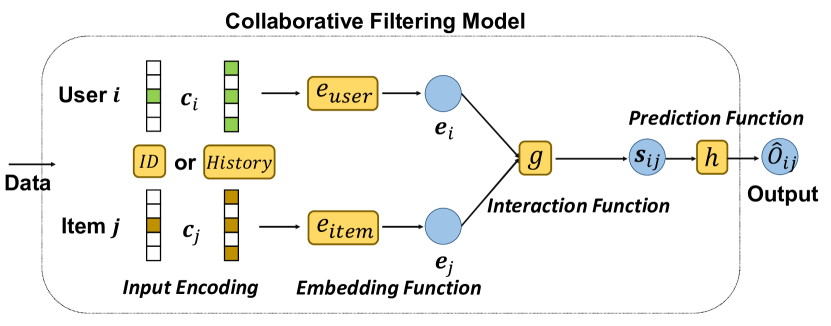
Figure 1. A unified framework of CF models, which contain four stages: input encoding, embedding function, interaction function and prediction function.

Recently, Automated Machine Learning (AutoML) (Hutter et al., 2019; Yao and Wang, 2018) achieved great success in various machine learning tasks, e.g., neural architecture search (Zoph and Le, 2017; Pham et al., 2018; Liu et al., 2019b; Yao et al., 2019; Li and Talwalkar, 2019) and hyper-parameter optimization (Bergstra and Bengio, 2012; Li et al., 2017; Feurer et al., 2019; liu, 2021), we propose to search data-specific CF models by AutoML techniques. However, there are two-fold challenges for AutoML-based CF problem:

• First, it is challenging to design a proper search space that can not only cover existing human-crafted methods but also explore more models that have superior performance for a given dataset.

• Second, since the datasets’ properties are quite diverse, the search strategy is required to be efficient, robust and ease-to-use.

To solve the first challenge, we propose a general framework that unifies state-of-the-art CF models. In general, most machine learning models consist of three key stages, data encoding, representation learning, and prediction function. CF models also follow this paradigm but with one significant extra stage, user-item matching, which is required after the representation learning. To be more specific, CF’s key is to match users with proper items, and this additional stage matches user representations with item representations. Thus, the general framework for CF models consists of four stages (as in Figure 1). First, the model encodes the input of user and item. Second, the model uses dense vectors to represent them. Third, the model matches user representations and item representations. Finally, a prediction function obtains the score.

To solve the second challenge, we develop a robust, efficient, and easy-to-use search strategy, which is based on the random search and a performance predictor. To be specific, with random search from the above-designed search space and a performance predictor to fast evaluate the searched models, our approach can efficiently find powerful models in the space for different datasets.

Our contributions can be summarized as follows.

• We approach the problem of CF task with the new perspective of automated machine learning. Since it is data-specific, we design AutoML based method to search proper CF model for a given dataset.

• We propose a general search space based on a standard four-stage paradigm of human-designed models for CF, including input coding, embedding function, interaction function, and prediction function. The proposed search space can not only cover most of the human-crafted models but also find more models not still explored by human experts. We develop an effective search strategy, which is easy-to-use and robust, to search data-specific CF models.

• Extensive experiments on five real-world datasets demonstrate that our proposed approach can efficiently search powerful models that achieve the best recommendation performance, with improvements of 1.65% - 22.66%. Analysis of the searched models provides insightful guidance to help human expert design models for CF. Further empirical results verify the effectiveness in search space and strategy design.

Table 1. Representative Human-designed CF Models. (Single models refer to those with one group of user and item embeddings; for fused models, there are multiple embedding matrices for user and item, bringing more learnable parameters. Here we have $u_{i}=\texttt{MAT}(\mathrm{ID}(i))$ and $v_{j}=\texttt{MAT}(\mathrm{ID}(j))$, and we use $u_{i}$ and $v_{j}$ for better presentation.)

Category	Name	Model Formulation	User Enc. $c_{i}$	Emb. $e_{\text{user}}$	Item Enc. $c_{j}$	Emb. $e_{\text{item}}$	Interacton $g$	Prediction $h$
Single	MF	$\mathbf{u}_{i}\cdot\mathbf{v}_{j}$.	ID	MAT	ID	MAT	multiply	SUM
	FISM (Kabbur et al., 2013)	$\texttt{MAT}({\mathbf{r}_{i}})\cdot\mathbf{v}_{j}$	History	ID	MAT	MAT	multiply	SUM
	GMF (He et al., 2017)	$\texttt{VEC}(\mathbf{u}_{i}\odot\mathbf{v}_{j})$	ID	MAT	ID	MAT	multiply	VEC
	MLP (He et al., 2017)	$\texttt{MLP}(\mathbf{u}_{i};\mathbf{v}_{j})$	ID	MAT	ID	MAT	concat	MLP
	CMF (Hsieh et al., 2017)	$||\mathbf{u}_{i}-\mathbf{v}_{j}||$	ID	MAT	ID	MAT	minus	Norm
	DMF (Xue et al., 2017)	$\texttt{MLP}(\mathbf{r}_{i})\cdot\texttt{MLP}(\mathbf{r}_{j})$	History	MLP	History	MLP	multiply	SUM
	JNCF-Cat (Chen et al., 2019)	$\texttt{MLP}(\texttt{MLP}(\mathbf{r}_{i});\texttt{MLP}(\mathbf{r}_{j}))$	History	MLP	History	MLP	concat	MLP
	JNCF-Dot (Chen et al., 2019)	$\texttt{MLP}(\texttt{MLP}(\mathbf{r}_{i})\odot\texttt{MLP}(\mathbf{r}_{j}))$	History	MLP	History	MLP	multiply	MLP
Fused	NeuMF (He et al., 2017)	$\texttt{VEC}(\mathbf{u}_{i}\odot\mathbf{v}_{j})+\texttt{MLP}(\mathbf{u}_{i};\mathbf{v}_{j})$	ID	MAT	ID	MAT	multiply	VEC
			ID	MAT	ID	MAT	concat	MLP
	SVD++ (Koren, 2008)	$\mathbf{u}_{i}\cdot\mathbf{v}_{j}+\texttt{MAT}({\mathbf{r}_{i}})\cdot\mathbf{v}_{j}$	ID	MAT	ID	MAT	multiply	SUM
			History	MAT	ID	MAT	multiply	SUM
	DELF (Cheng et al., 2018)	$\texttt{MLP}(\mathbf{u}_{i};\mathbf{v}_{j})$	ID	MAT	ID	MAT	concat	MLP
		$+\texttt{MLP}(\mathbf{u}_{i};\texttt{MLP}(\mathbf{r}_{j}))$	ID	MAT	History	MAT	concat	MLP
		$+\texttt{MLP}(\texttt{MLP}(\mathbf{r}_{i});\mathbf{v}_{j})$	History	MAT	ID	MAT	concat	MLP
		$+\texttt{MLP}(\texttt{MLP}(\mathbf{r}_{i});\texttt{MLP}(\mathbf{r}_{j}))$	History	MAT	History	MAT	concat	MLP

Notation

The dataset utilized in the CF task is a user-item interaction matrix $\mathbf{Y}^{M\times N}$ with $M$ users and $N$ items. Each entry of this matrix can be binary or ratings (from 1 to 5, for example). The objective of CF is to estimate the missing values of the matrix. In other words, the output of a CF model is $\hat{\mathbf{O}}_{ij}$ for user $u$ and item $j$. MAT$(\cdot)$ represents to multiply the multi-hot representation with a matrix and then apply to mean pooling; since the embedding lookup for ID and embedding lookup for history with mean pooling are quite similar, both of them are denoted with MAT. For the final prediction, SUM denotes multiply with an all-one vector (i.e., sum), VEC denotes multiply with a learnable vector, and MLP stills denotes feeding a multi-layer perception. We use $(\cdot;\cdot)$ to denote a concatenation operation and $\odot$ to denote the element-wise product.

2. Related Work

2.1. Collaborative Filtering (CF)

Collaborative filtering (CF) (Sarwar et al., 2001; He et al., 2017), learning user preferences based on user-item interaction, is the most fundamental solution for recommender systems. Memory-based CF (Sarwar et al., 2001) is the earliest CF approach that calculates the similarity of the whole interaction history. Recently, model-based CF which builds latent factor models with learnable parameters and predicts users’ preference score towards items directly, becomes more popular. We summarize the representative CF models in Table 1. MF et al. (Koren, 2008) was proposed to project user ID and item ID with real-value vectors, representing user interests and item features, respectively. Then MF uses the inner product to predict the preference score with user and item embeddings. CMF et al. (Hsieh et al., 2017) was proposed that uses minus operation to replace MF’s inner product.

Beside IDs, user history and item history can also be used to represent the encoding, which has been demonstrated effective in SVD++ (Koren, 2008), FISM (Kabbur et al., 2013) and SLIM (Ning and Karypis, 2011). These early progresses only use explicit rating data, such as user-movie rating scores. However, in modern recommender systems, there is plenty of implicit feedback data, such as the purchase or click records. Therefore, the item-ranking task, which takes the implicit data as input and predicts a ranking list, is more important. BPR (Rendle et al., 2009) proposed a pairwise learning manner to optimize the MF model on implicit data. Inspired by the big success of the deep neural networks in computer vision and natural language processing (LeCun et al., 2015), NCF (He et al., 2017) applied neural networks to building CF models. NCF used a multi-layer perceptron (MLP) as the interaction function, taking user and item embedding vectors as input and predict the preferences score. Similarly, DeepMF et al. (Xue et al., 2017) proposed a deep matrix factorization model that replaced user/item ID with user/item history and reserved the inner product operation in MF. Furthermore, JNCF et al. (Chen et al., 2019) extended NCF by using user/item history to replace user/item ID as the input encoding. The authors proposed two variants, JNCF-Cat and JNCF-Dot, with different functions to match user embeddings and item embeddings. There is a recent work, SIF (Yao et al., 2020), that adopts the one-shot architecture search for adaptive interaction function in the CF model.

Recently, researchers found that the neural model does not necessarily perform better than shallow models (Dacrema et al., 2019). In other words, whether a model is suitable or not largely depends on the dataset. Since CF tasks are various, on totally different datasets with diverse properties, the best model could be different. In other words, designing models for CF is a data-specific problem.

2.2. Automated Machine Learning (AutoML)

Automated machine learning (AutoML) (Hutter et al., 2019; Yao and Wang, 2018) refers to a type of method that can self-adapt machine learning models to various tasks. Recently, AutoML has achieved a great success in designing the state-of-the-art model in various learning applications such as image classification/segmentation (Zoph and Le, 2017; Tan and Le, 2019; Liu et al., 2019a), natural language modeling (So et al., 2019), and knowledge graph embedding (Zhang et al., 2019). A general framework of AutoML consists of three parts as follows:

• Search Space: it defines the set of all possible models, which be finite or infinite. Search space is designed with human expertise on specific applications. The search space should be carefully chosen since an overlarge space brings challenges to model search will a too-small space cannot cover powerful models.

• Search Algorithm: it refers to the algorithm that guides the searching process in the space. Popular choices are random search (Bergstra and Bengio, 2012), evolutionary algorithms (Xie and Yuille, 2017), Bayesian optimization (Bergstra et al., 2011) and reinforcement learning (Zoph and Le, 2017). Among them, while being simple, random search is a strong baseline in many applications (Bergstra et al., 2011; Li and Talwalkar, 2019).

• Model Evaluator: it measures the performance of a candidate, i.e., a model, in the space, which is also usually the most expensive part in AutoML. The most basic evaluator is direct model training. Early-stop (Maron and Moore, 1994; Hutter et al., 2011) is a popular trick to cut-down training cost of bad candidates. Performance predictor (Eggensperger et al., 2015; Liu et al., 2018; Zhang et al., 2019) extended it by avoid training of unpromising candidate via an additional model.

Since search space requires a lot of domain-specific knowledge, it is very diverse for current AutoML applications, e.g., from shallow models (Thornton et al., 2013; Feurer et al., 2019; Zhang et al., 2019) to deep neural architectures (Pham et al., 2018; Zoph and Le, 2017). Search algorithm and model evaluator highly couple with each other. Specifically, the search algorithm focuses on generating the next candidates in the search space, while the evaluator offers feedbacks to the algorithm. Thus, the computational cost of AutoML depends on both the number of candidates generated (by the algorithm) and the evaluating time of candidates (by the evaluator).

3. Problem Definition

As mentioned in the introduction, designing CF models is data-specific. Based on the proposed framework, we propose to use AutoML to efficiently search CF model for the given dataset.

3.1. A Unified Framework of CF Model

As mentioned in the introduction, CF models also follows the paradigm of general machine learning, i.e., data encoding, representation learning, and prediction function, while one significant additional stage, user-item matching, is required after the representation learning. To be more specific, the key to CF is to match users with proper items, and this additional stage matches user representations with item representations. In general, the four stages derived from existing CF models are in Figure 1 and details are as follows:

1. Input encoding represents the input of user and item. The two main choices are ID-based one-hot encoding or history-based multi-hot encoding, which represents a user with her historically interacted items (i.e. one row in user-item interaction matrix), as follows,

   (1) $$\mathbf{c}_{i}=\mathrm{ID}(i)\,\,\mathrm{or}\,\,\mathbf{r}_{i},$$

   $$\mathbf{c}_{j}=\mathrm{ID}(j)\,\,\mathrm{or}\,\,\mathbf{r}_{j},$$

   where $\mathbf{r}_{i}$ ($\mathbf{r}_{j}$) is $i$-th row ($j$-th column) of the user-item matrix.

2. Embedding function projects the input encoding to dense real-value embeddings, which represent the user interests or item features, denoted as $\mathbf{e}_{i}$ and $\mathbf{e}_{j}$ respectively, as follows,

   (2) $$\mathbf{e}_{i}=e_{\text{user}}(\mathbf{c}_{i}),\quad\mathbf{e}_{j}=e_{\text{item}}(\mathbf{c}_{j}),$$

3. Interaction function matches the user and item embeddings in the latent space for further prediction, as follows,

   (3) $$\mathbf{s}_{ij}=g(\mathbf{e}_{i},\mathbf{e}_{j}).$$

4. Prediction function converts the output of interaction function into predicted value of user-item preferences, as follows,

   (4) $$\hat{\mathbf{O}}_{ij}=h(\mathbf{s}_{ij}).$$

Here we present some empirical results to reveal each stage’s significant impact on recommendation performance (see full results in Table 3 and Table 4). FISM (Kabbur et al., 2013) that utilizes user history as input encoding performs better than MF in some tasks (item ranking), while fails in others. The similar finding can also be observed in the interaction function by comparing CMF (Hsieh et al., 2017) and MF and in the prediction function by comparing GMF (He et al., 2017) and MF. The impact of four stages’ operation choices is in two folds. First, a bad choice of any stage may make the whole recommendation model not work at all. Second, whether the choice of each stage is good or not is closely related to the specific datasets, as datasets’ different properties require different operations. As a result, the design of CF model is a data-specific problem involving the operation selection of four stages.

3.2. Formulating as an AutoML Problem

Recently, researchers found that neural models do not necessarily perform better than shallow models (Dacrema et al., 2019), which makes us rethink the CF task. Since CF tasks are various, with totally different datasets and performance measurement, the best model should be different. There is no one-for-all model that can always achieve good performance on all CF tasks. In other words, model design for CF is a data-specific problem. As discussed above, since different datasets’ properties have a significant impact on the performance of CF models, we are motivated to form the problem of designing new and better CF models as a search problem, as follows:

Definition 1 (Automated Model Search for CF (AutoCF)).

Let $f^{*}$ denote the desired CF model. Then the CF search problem can be formulated as:

(5) $$f^{*} =\max\nolimits_{f\in\mathcal{F}}\mathcal{M}(f(\mathbf{P}^{*}),\mathcal{S}_{\text{val}}),$$

(6)  s.t. $$\mathbf{P}^{*}=\operatorname*{arg\,max}\nolimits_{\mathbf{P}}\mathcal{M}(f(\mathbf{P}),\mathcal{S}_{\text{tra}}),$$

where $\mathcal{F}$ contains all possible choices of $f$, $\mathcal{S}_{\text{val}}$ and $\mathcal{S}_{\text{tra}}$ denote the training and validation datasets, $\mathbf{P}$ denotes the learnable parameters of the CF model $f$, and $\mathcal{M}$ denotes the performance measurement.

To solve the AutoCF problem well, there are two important aspects. First, the search space should cover various operations, which make sure for capturing various characteristics of different datasets. Second, the search strategy should be both robust and efficient that can meet the requirements of both accuracy and efficiency in real-world applications.

Compared with previous AutoML solutions (Tan and Le, 2019; Liu et al., 2019b; Liu et al., 2019a), the AutoCF problem is quite different since the search space and strategy are closely related to the domain of personalized recommender systems. First, both shallow and deep models are demonstrated to be effective by existing works (He et al., 2017; Dacrema et al., 2019). Second, the task’s settings in real-world applications are diverse, which requires an efficient search strategy to search powerful models for a given dataset.

4. Our Approach

Following a commonly-recognized paradigm of AutoML, solving the AutoCF problem should consider three parts, search space, search algorithm, and model evaluator, as mentioned in Section 2.2. Our AutoCF approach is featured as follows:

• A general search space, i.e., $\mathcal{F}$, that not only covers effective state-of-the-art solutions, but also explores new models.

• An easy-to-use and robust search strategy including 1) a random search algorithm that is simple yet effective and 2) a performance predictor based model evaluator to help fast evaluate the searched models.

Recently, SIF (Yao et al., 2020) propose a one-shot architecture search algorithm for finding good interaction functions in rating prediction tasks. In this work, we consider the problem from a more general perspective, besides the interaction function, with a full model search including input encoding, embedding function, interaction function, and prediction function, on both implicit and explicit feedback data. In addition, the search algorithm in (Yao et al., 2020) cannot be applied to searching full CF models for our problem since it can only search operations with the same input/output.

4.1. Search Space Design

To solve the challenge of search space design, we unify the state-of-the-art CF models in a general framework, which follows a four-stage paradigm.

4.1.1. Operation Selection

The used operations for the search space are illustrated in Table 2.

Input Encoding There are no extra features in CF tasks, such as user profiles or item attributes; thus, for representing user and items, an intuitive manner is ID, using the one-hot ID and maintaining two embedding matrices. Another manner is History, to represent a user with his/her multi-hot history (i.e. interacted items), and items can be represented similarly. That is, encoding refers to how to represent the user and item in the CF task.

Embedding Function Embedding function that projects the high-dimensional input encoding to low-dimension embeddings is closely related to input encoding operation. With ID input encoding, the only compatible embedding function for user/item is user/item embedding matrix ID-look-up, denoted as MAT. With history input encoding, there are two kinds of compatible embedding functions. First, the user/item embedding function of item/user embedding matrix ID-lookup and mean pooling is used in some representative models such as FISM (Kabbur et al., 2013) and SVD++ (Koren, 2008), denoted as MAT. The item embedding function can be built similarly. Second, a multi-layer perceptron can also be used to convert multi-hot history into dense vectors directly, denoted as MLP. Here for the architecture of MLP, we follow the setting in the state-of-the-art neural model, NeuMF (He et al., 2017).

Interaction Function Interaction function connect two sides, i.e., user and item, for subsequent prediction. A frequently-used interaction function is to use element-wise product, multiply, to generate a combined vector. Similar operation consists of minus, max, min and concat.

Prediction Function The prediction function converts the output of the interaction function to a predicted score. A simple yet effective operation is summation, denoted as SUM. Inner product with a weight vector can be used to assign weights to a different dimension, denoted as VEC. The multi-layer perceptron can also be used for more complicated prediction, denoted as MLP.

4.1.2. Full Model Encoding

For a whole model, we need to define an encoding to represent the above choices of each stage. Since one-hot representation has been demonstrated effective by previous works (Zhang et al., 2019; Liu et al., 2018), we adopt it to represent each stage’s operation. To make the space more general, we also consider embedding dimension choice from a set $\mathcal{S}_{\text{dim}}$ and optimizer’ learning rate from a set $\mathcal{S}_{\text{lr}}$ as part of the encoding. Then size of the whole space is $135*|\mathcal{S}_{\text{dim}}|*|\mathcal{S}_{\text{lr}}|$. For example, $(\{0,1\}$, $\{1,0\}$, $\{1,0\}$, $\{0,1\}$, $\{0,0,1,0,0\}$, $\{1,0,0\}$, $\{0,0,1,0\}$, $\{0,1,0,0\})$ represents the model with (History, ID, MAT, MLP, min, SUM) learned with $3$-th embedding dimension size and $2$-th learning rate choice, if the size of $\mathcal{S}_{\text{dim}}$ and $\mathcal{S}_{\text{lr}}$ are both set to $4$. This corresponds the whole paradigm in Figure 1 and operation choice in Table 2.

Table 2. The operations we use for the search space.

Stage	Operations
Input Encoding	User	ID, History
	Item	ID,  History
Embedding Function	User	Mat,  MLP
	Item	Mat,  MLP
Interaction Function	MUL,  MINUS,  MIN,  MAX,  CONCAT
Prediction Function	SUM,  VEC,   MLP

4.2. Search Strategy

To solve the challenge of search efficiency, we propose an easy-to-use and robust search strategy that combines random search with performance predictor. The whole search strategy is present in Algorithm 1. Given the defined search space, our problem turns to design efficient and proper search strategy to find models with excellent performance. Note that our problem is also suffering the problem of discrete search space, and thus random search, which is a strong baseline in many AutoML applications (Li and Talwalkar, 2019; Zoph and Le, 2017; Sciuto et al., 2020), can be a simple and effective solution.

However, the evaluation in random search is expensive. To make the search process efficient, we propose to combine random search with a performance predictor that can quickly evaluate the performance of searched models.

4.3. Experimental Settings

Table 3. Comparison on Rating-Prediction Task.

Dataset		MovieLens-100K		MovieLens-1M		Yelp		Amazon-Book
Metric		RMSE	MAE	RMSE	MAE	RMSE	MAE	RMSE	MAE
Single	MF	0.8964	0.4906	0.8152	0.7061	1.1031	0.8204	1.0661	0.9910
Model	FISM	0.9212	0.4645	1.0379	0.9516	1.0746	1.2510	1.0265	1.1273
	GMF	0.8872	0.4993	1.2125	1.0259	1.0413	0.7473	1.0249	0.9148
	MLP	0.8632	0.4665	0.8135	0.6588	0.9218	0.6598	0.8803	0.7565
	DMF	0.5118	0.4682	0.8043	0.6577	0.9051	0.6587	0.8458	0.7563
	JNCF-Dot	0.4703	0.4146	0.7946	0.6101	0.9084	0.6553	0.8469	0.7620
	JNCF-Cat	0.4587	0.4124	0.7990	0.6041	0.9029	0.6559	0.8454	0.7534
	CMF	0.7151	0.4232	1.2688	0.8722	1.4401	1.0088	1.3474	1.2708
	AutoCF	0.4479	0.3876	0.7933	0.5911	0.9012	0.6410	0.8431	0.7351
	Improvement	2.24%	6.01%	1.65%	2.15%	2.18%	4.56%	3.65%	3.35%
Fused	SVD++	0.8809	0.4244	0.8295	0.6708	1.0710	0.7449	0.9945	0.8334
Model	NeuMF	0.7923	0.4590	0.7909	0.7366	0.9910	0.7673	0.9259	0.8729
	DELF	0.5357	0.3912	0.7904	0.8036	0.9807	0.8553	0.9106	0.8538
	SinBestFuse	0.4215	0.3942	0.7827	0.6038	0.8994	0.6429	0.8368	0.7356
	AutoCF	0.4075	0.3516	0.7744	0.5861	0.8805	0.6233	0.8235	0.7155
	Improvement	10.96%	11.08%	10.99%	11.21%	10.98%	11.30%	11.01%	11.18%

1

2

input : Search space $\mathcal{F}$, a learnable predictor $\mathcal{P}$, performance measurement $\mathcal{M}$, a empty set $\mathcal{H}$, size of training batch for predictor $K_{1}$ and $K_{2}$, training data $\mathcal{S}$.

3

4Initialize the predictor $\mathcal{P}$ with random parameters;

5

6do

7       Randomly select a $(K_{1}+K_{2})$-size model set $\mathcal{F}^{b}$ from $\mathcal{F}$;

8       Generate one-hot encodings $\mathbf{x}_{o}$ to represent models in $\mathcal{F}^{b}$;

9       Estimate the performance of models in $\mathcal{F}^{b}$ with $\mathcal{P}$ ;

10       Choose top-$K_{1}$ model sets $\mathcal{F}^{t}$ to train with $\mathbf{\mathcal{S}}$;

11       Evaluate the trained models in $\mathcal{F}^{t}$ with $\mathbf{\mathcal{M}}$ ;

12       Update the set of evaluated-model $\mathcal{H}\leftarrow\mathcal{H}\cup\{(f,\mathcal{M}(f))|f\in\mathcal{F}^{t}\}$ ;

13       Update $\mathcal{P}$ with records in $\mathcal{H}$ via loss function in (8).

14while not meet stop criteria;

return desired CF models in $\mathcal{H}$.

Algorithm 1 AutoCF: Automated Model Search for CF

4.3.1. Predictor Design

However, the bottleneck in our problem is the evaluation of models. Inspired by previous AutoML works (Eggensperger et al., 2015; Liu et al., 2018; Zhang et al., 2019), we propose a predictor to distinguish good and bad models. Predictor, as mentioned in Section 2.2, is a model that can estimate the performance given each model’s features without training.

It is worth mentioning that many previous AutoML tasks utilize weight-sharing techniques (Liu et al., 2019b; Pham et al., 2018) to accelerate model evaluator. For example, the searched different CNN models can share parameters in the a cell without re-training in (Pham et al., 2018). However, in our AutoCF problem, the search space cannot be constructed to a super net (a directed acyclic graph (DAG) of which a path denotes a single model) (Pham et al., 2018) due to the disjoint stages of CF models, which makes the weight-sharing technique cannot be applied.

Predictor aims to predict performance given a model, and thus we need to represent each one in the space with unique encoding. As introduce in Section 4.1, the encoding is denoted as $\{\mathbf{x}_{o}\}$ with $o$ from $1$ to $4$. As discussed in Section 2.2, multi-layer perceptron and tree-based models such as random forest are the two mainstream models for predictor. In our problem, the multi-layer perceptron supports parameter updates with gradient descent, which is more compatible with random search and has a stronger ability to learn from complex data. Thus, we use a multi-layer perceptron to predict the model’s performance based on the encodings, as follows,

(7) $$\mathcal{P}(\mathbf{x}_{o})=\text{\tt MLP}(\text{\tt Concat}(\mathbf{x}_{o})),$$

where the predicted recommendation performance can be in various forms, such as rating prediction accuracy or ranking recall.

4.3.2. Predictor Training

For finding good models efficiently, it is not necessary to predict the absolute value of a specific metric since it is more meaningful to distinguish the better model with several candidates. Therefore, we train the predictor with pairwise loss (Rendle et al., 2009). To be specific, the predictor’s objective is to rank pairs with the right order based on evaluated models. The loss function is formulated as follows,

(8) $$L_{\mathcal{P}}=\sum\nolimits_{(\mathbf{x}_{+},\mathbf{x}_{-})\in O}-\log\big{(}\sigma(\mathcal{P}(\mathbf{x}_{+})-\mathcal{P}(\mathbf{x}_{-}))\big{)},$$

where $O$ are built pairs that consists of two searched architectures, and $\sigma$ denotes the sigmoid function. $\mathbf{x}_{+}$ and $\mathbf{x}_{-}$ denotes the model encoding of the better architecture and the worse one, respectively.

In short, a standard job procedure is first sampling models from the space and then utilizing the predictor to choose top models for real evaluation, and lastly, using evaluation results to update the predictor. This job procedure is repeated under random search until finding powerful models for a given task.

When the pipeline stops (stop criteria can be a hyper-parameter and chosen for different purposes), we obtain a valid predictor that can predict all models’ performance with high accuracy and find effective models from the search space.

5. Experiments and Evaluations

The mainstream recommendation tasks can be divided into two categories, rating prediction, and item ranking. Based on these two categories, we conduct experiments to answer the following research questions.

• Can our method find data-specific CF models that outperform human-design ones on benchmark datasets?

• What insights can we see from searched models?

• How about our designed search space compared with other possible search space? How can the designed predictor speed up search algorithms?

5.0.1. Datasets

In the experiments, we use MovieLens-100K, MovieLens-1M, Yelp, and Amazon-Book for the rating-prediction task, and use MovieLens-100K, MovieLens-1M, Yelp, and Pinterest for the item-ranking task. The details, including statistics, of datasets are shown in Appendix A.4.

5.0.2. Metrics and Loss Function

As the objective of two tasks is different, metrics for evaluating recommendation models are also different. For the task of rating prediction, we use the following two widely used standard metrics of RMSE and MAE (Chai and Draxler, 2014).

While for the task of item ranking, the mainstream evaluation metrics can be divided into two kinds, recall-ratio based metrics such as Recall and Hit Ratio and rank-position based metrics such as NDCG and MRR (Manning et al., 2008). Here we choose two most widely used metrics, Recall and NDCG.

Similarly, the choice of the loss function is also different for two kinds of tasks. For rating prediction CF tasks, we adopt the widely-used utilized loss function of RMSE loss (Koren, 2008); while for item ranking CF tasks, we adopt the BPR loss (Rendle et al., 2009), the state-of-the-art loss function for optimizing recommendation models.

5.0.3. Hyper-parameters

Besides the above-mentioned search space, there are also two hyper-parameters for each model: optimizer and negative sampler. For both two tasks, we choose Adam (Kingma and Ba, 2015) optimizer. For item ranking tasks, we need to sample some unobserved items as negative feedback, of which the choice of the negative sampler is another hyper-parameter. For our experiments, we use the most acceptable random negative sampler (He et al., 2017; Kabbur et al., 2013; Rendle et al., 2009) that randomly chooses one unobserved item as a negative sample for each observed user-item feedback.

Table 4. Comparison on Item-Ranking Task.

Dataset		MovieLens-100K		MovieLens-1M		Yelp		Pinterest
Metric		Recall@20	NDCG@20	Recall@20	NDCG@20	Recall@20	NDCG@20	Recall@20	NDCG@20
Single	MF	0.1073	0.1345	0.0990	0.0589	0.0870	0.0486	0.0965	0.0645
Model	FISM	0.1572	0.1422	0.1097	0.0627	0.0928	0.0516	0.1022	0.0703
	GMF	0.1047	0.1412	0.1092	0.0619	0.0939	0.0499	0.1011	0.0691
	MLP	0.1358	0.1221	0.0929	0.0542	0.0807	0.0430	0.0868	0.0602
	DMF	0.1833	0.1213	0.0940	0.0352	0.0800	0.0428	0.0876	0.0602
	JNCF-Dot	0.2067	0.1448	0.1255	0.0640	0.0954	0.0503	0.1027	0.0705
	JNCF-Cat	0.1875	0.1454	0.1221	0.0642	0.0961	0.0517	0.1045	0.0705
	CMF	0.1450	0.1091	0.0830	0.0489	0.0707	0.0384	0.0778	0.0523
	AutoCF	0.2327	0.1755	0.1346	0.0785	0.1155	0.0633	0.1255	0.0862
	Improvement	21.64%	21.20%	21.26%	22.66%	21.07%	22.44%	20.10%	22.27%
Fused	SVD++	0.1774	0.1340	0.1028	0.0599	0.0873	0.0470	0.0949	0.0654
Model	NeuMF	0.2114	0.1583	0.1215	0.0695	0.1042	0.0567	0.1124	0.0783
	DELF	0.1931	0.1453	0.1121	0.0642	0.0952	0.0511	0.1038	0.0711
	SinBestFuse	0.2585	0.1934	0.1479	0.0864	0.1264	0.0697	0.1390	0.0940
	AutoCF	0.2904	0.2190	0.1677	0.0973	0.1425	0.0777	0.1554	0.1065
	Improvement	12.34%	13.24%	13.39%	12.62%	12.74%	11.48%	11.80%	13.30%

Table 5. Top 3 searched models of each dataset. H represents History.

Task	Dataset	Top1	Perf.	Top2	Perf.	Top3	Perf.
	ML-100K	$\big{<}$H,H,MLP,MLP,max,MLP$\big{>}$	0.4479	$\big{<}$H,H,MLP,MLP,max,VEC$\big{>}$	0.4512	$\big{<}$H,H,MLP,MLP,min,MLP$\big{>}$	0.4520
Rating Prediction	ML-1M	$\big{<}$H,H,MLP,MLP,multiply,VEC$\big{>}$	0.7933	$\big{<}$H,H,MAT,MLP,min,MLP$\big{>}$	0.7939	$\big{<}$H,H,MLP,MLP,max,MLP$\big{>}$	0.7945
(RMSE)	Yelp	$\big{<}$H,H,MLP,MLP,plus,SUM$\big{>}$	0.9012	$\big{<}$H,H,MLP,MLP,concat,SUM$\big{>}$	0.9015	$\big{<}$H,H,MLP,MAT,min,SUM$\big{>}$	0.9021
	Amazon-book	$\big{<}$ID,H,MLP,MLP,max,VEC$\big{>}$	0.8431	$\big{<}$ID,H,MLP,MLP,min,VEC$\big{>}$	0.8432	$\big{<}$ID,H,MAT,MLP,concat,VEC$\big{>}$	0.8447
	ML-100K	$\big{<}$H,H,MAT,MAT,multiply,VEC$\big{>}$	0.2327	$\big{<}$H,H,MAT,MAT,multiply,MLP$\big{>}$	0.2197	$\big{<}$H,H,MLP,MLP,min,VEC$\big{>}$	0.2149
Item Ranking	ML-1M	$\big{<}$H,H,MAT,MAT,multiply,VEC$\big{>}$	0.1346	$\big{<}$H,H,MLP,MLP,min,MLP$\big{>}$	0.1282	$\big{<}$H,H,MLP,MLP,multiply,MLP$\big{>}$	0.1255
(Recall@20)	Yelp	$\big{<}$H,H,MLP,MLP,multiply,VEC$\big{>}$	0.1155	$\big{<}$H,H,MAT,MAT,multiply,VEC$\big{>}$	0.1091	$\big{<}$H,H,MLP,MLP,min,VEC$\big{>}$	0.1077
	Pinterest	$\big{<}$H,H,MAT,MAT,multiply,SUM$\big{>}$	0.1255	$\big{<}$H,H,MAT,MAT,multiply,MLP$\big{>}$	0.1210	$\big{<}$H,H,MLP,MLP,min,VEC$\big{>}$	0.1169

5.1. Benchmark Performance Comparison

5.1.1. Single Model Comparison

According to the definition in Section 2, single models only use one group of embeddings for users and items. Here we choose the nine mainstream single models introduced in Section 2.1 for comparison. Note that all methods can be adapted to two tasks by transforming loss function, even if they may be designed for one task, e.g., NCF (He et al., 2017) is originally proposed for item ranking tasks.

We present the obtained RMSE and MAE performance in Table 3. From the results, we can observe that our proposed method searches a model achieving the best performance on all metrics across the four datasets. The improvement is steady for different datasets, and our proposed method can outperform the best baseline by 1.65% to 6.01%, which demonstrate the our approach can effectively self-adapt to different tasks to find powerful models. Another interest observation is that JNCF-Cat, as the best baseline, outperforms all other baselines. This can be explained that use rating-history can introduce more useful signals for embeddings. In other words, the rating-history can be considered as a kind of feature input. For this, we will conduct more analysis in Section 5.3.

For the item ranking tasks, we use the full-ranking protocol (Rendle, 2019) to calculate the Recall@K and NDCG@K. Precisely, for each test item, we first calculate the interaction probability of all unobserved items (excepted for items sampled for pair-wise learning); then, we rank the predicted scores for metric calculation. Here we set K to 20, following common settings of many recent works (Wang et al., 2019a, b). We present the performance on four utilized datasets in Table 4. It is worth mentioning that there are differences between our results and original papers for two reasons. First, the data splitting and pre-processing always have some differences. Second, the ranking metrics are highly relevant to the length of the list and the choices of top-K. In our experiments, we choose the full-ranking, which is a more reasonable choice, which makes our results have large difference compared with those sampling-ranking papers (He et al., 2017).We can observe that our searched models can achieve the best performance compared with all other baselines. Note that our proposed method can outperform the best baseline by 20.10% to 22.66%.

5.1.2. Fused Model Comparison

Some researches also find the strong power of model fusion in CF. In the original paper of NCF, the authors propose a model named NeuMF that fusion a generalized MF and MLP together. Cheng et al. (Cheng et al., 2018) proposed a dual model named DELF that fusions four extensions of MLP as a whole model.

Although those fused models can achieve better performance, their larger parameter size and training/inferring cost are always a concern. For better comparison, we also fuse the top-2 best single models, comparing with the recent advances in recommender systems, which also fuses two single models: SVD++ fuses MF and FISM, NeuMF fuses GMF and MLP, and DELF fuses several MLP-based models. We also choose the top-2 baselines in single-model experiments and fuse then as a competitive baseline method, denoted as SinBestFuse.

We present the performance of rating prediction and item ranking in Table 3 and 4. We can easily find that our fused model can achieve the best performance, improving the best baseline by 10.96%-13.39%. In short, with model fusion that can take advantage of different good models in the space, the recommendation performance can be further improved.

5.2. Case Study: Data-specific Models

For the searched models, we present the top ones for each task on all datasets in Table 5. In general, the searched models of different tasks are quite different, which further validates the necessity of considering CF as a data-specific problem. We can find that for these top models of each task, there are always similar input encoding. Another finding is that the impact of the prediction function is the smallest. On the ML-100K datasets, the top-2 models even only differ in prediction function. In order to present the impact of each stage more clearly, we conduct the analysis of each one as follows,

• Input Encoding. Most top-models have a common CF prediction signal, $\{\texttt{History},\texttt{History}\}$. However, for the Amazon-Book dataset, models with $\{\texttt{ID},\texttt{History}\}$ as the raw input of embedding function can also achieve good performance. This can be explained that user-side records in Amazon-book are more sparse than other datasets.

• Embedding Function. For different tasks, the choice of embedding function has big differences. We can observe that MLP tend to perform better in the rating prediction task, while MAT can achieve good performance in item ranking tasks. This verifies that our method can distinguish the difference and select suitable operations for different tasks.

• Interaction Function. For the interaction function, we can first find that our method can choose the proper one for two different tasks on different datasets. Furthermore, for MovieLens-100K where exists a larger popularity bias, interaction functions can learn non-personalized bias such as min and max can achieve good performance.

• Prediction Function. For the choice of prediction function, sparse datasets tend to choose simple VEC or SUM, which have few parameters and is easy to learn.

Table 6. Comparison of search algorithms with/without predictor.

		Number of Evaluated Models.
Task	Dataset	Rand	Reinforce	Rand(P)	Reinforce(P)	Reduction
Rating Prediction	ML-100K	1,420	1,450	150	170	89.44%
	ML-1M	1,450	1,250	370	360	74.48%
	Yelp	1,310	1,180	450	470	65.65%
	Amazon-book	1,420	1,390	520	530	63.38%
Item Ranking	ML-100K	1,250	1,170	360	400	71.20%
	ML-1M	1,510	1,470	330	350	78.15%
	Yelp	1,240	1,240	510	500	58.87%
	Pinterest	1,570	1,570	500	530	68.15%

In summary, the best models are not the same for different datasets but sharing some powerful choice of operations, such as input encoding. These results, along with analysis, can inspire human experts to design more powerful models.

5.3. Ablation Study

5.3.1. Plausibility of the Search Space

To further validate the effectiveness of our designed search space, we propose to extensively search the architectures for the state-of-the-art model, NeuMF (He et al., 2017), with reinforcement learning-based controller (Zoph and Le, 2017). As described in (He et al., 2017), the architecture of multi-layer perceptrons can have many implementations. With an extensive architecture search, we present the performance comparison of the best-searched model in Table 7. From these results, we can find our search space can always obtain better architectures compared with NeuMF’s space for different CF tasks. Under our designed search space, the best method can improve NeuMF+NASNet by 1.11%-35.00% for different tasks. As the discussion in Section 2.1, it was found (Dacrema et al., 2019) deep models do not necessarily perform better performance compared with shallow models. Our empirical results further validate this observation. In summary, we conclude that our designed search space is more proper for CF tasks and cover more powerful models, based on the observed performance improvement.

Table 7. Performance comparison of different search space.

		Best Performance in Search Space
Task	Dataset	NeuMF+NASNet	AutoCF	Improv.
Rating	ML-100K	0.6754	0.4075	35.00%
Prediction	ML-1M	0.7831	0.7744	1.11%
(RMSE)	Yelp	0.9530	0.8805	7.60%
	Amazon-book	0.8640	0.8235	4.69%
Item	ML-100K	0.2327	0.2904	24.79%
Ranking	ML-1M	0.1399	0.1677	14.36%
(Recall@20)	Yelp	0.1121	0.1425	27.18%
	Pinterest	0.1218	0.1554	27.58%

5.3.2. Acceleration from the Predictor

In this work, we propose a predictor based search strategy that can find effective models in space. Here we replace the random search with Reinforce (Zoph and Le, 2017). Reinforce (Zoph and Le, 2017) is the most widely used search strategy in the neural architecture search. To adapt it to our problem, we design a multi-layer perceptron as the controller of which the output is the operation choice. By using the recommendation performance of the sampled models as a reward, we adopt the policy gradient (PG) to update the controller. Here we combine it with our proposed performance predictor and named it as Reinforce(P).

We present the cost of evaluation of our search strategy in Table 6. The details of rating prediction task on ML-1M is shown in Figure 2. The cost is measured by the number of evaluated models before finding the best model. We can find that compared with two baseline methods, our proposed search strategy is quite efficient, improving the best baseline by 58.9%-89.4%. We can observe that the Reinforce search algorithm has quite a similar search efficiency with the random search without predictor. This further validates our discussion in Section 2.2: for those tasks of which the search space is discrete, the problem on evaluation (for the lower-level problem) may be more critical than the choice of search algorithm (for the lower-level problem). In summary, our search algorithm is efficient and has high application value.

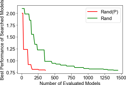
Figure 2. Test RMSE curve with or without predictor.

6. Conclusion and Future Work

In this work, we consider the model design in CF as a data-specific problem and approach this problem with automated machine learning. With an elaborately designed search space and efficient search strategy, our AutoCF approach can generate better models than human-designed baselines with various datasets in multiple real-world applications. Our proposed predictor is demonstrated to be more efficient compared with the existing search strategy. Further experiments verify the rationality of our designed search space. The case study on searched powerful models provide insights for developing CF models. First, some operation choices always achieve good performance, such as using history as the input encoding; second, there are some operations mainly depending on the datasets.

For the future work, we plan to transfer the searched top models in our utilized datasets to datasets with an industrial scale. This will make our approach an effective solution to handle the CF model design in very large datasets. Another important future work is to expand the definition of CF to cover more possible operations, including embedding propagation operation (Wang et al., 2019b). We also plan to consider more extensive recommendation tasks besides CF, such as content-based recommendation (Rendle, 2010).

7. Acknowledgments

This work was supported in part by The National Key Research and Development Program of China under grant 2020AAA0106000.

Appendix A Appendix for reproducibility

A.1. Search Space

Since the hyper-parameter of the CF model can also be regarded as a part of the model from the perspective of AutoML. In our experiments, we consider learning rate and embedding size as a component of the search space. Thus, the whole search space, including the choices of user/item input encoding, user/item embedding function, interaction function, prediction function, embedding size, and learning rate. This makes there are eight one-hot encodings to represent the choice of each component.

A.2. Search Strategy

In our approach, we have some key hyper-parameters. For the size of the sampled model set, we set $K_{1}$ and $K_{2}$ as 10 and 10. We have also tried other settings and find the difference is minor. The stopping criterion of our approach is set to no improvement for 100 samples after beating state-of-the-art human-crafted models. The MLP predictor is set to be 2-layer MLP, with embedding size as {8, 4}, with a few parameters since the size of one-hot encodings of each model is not large.

For the training of our MLP predictor, the learning rate is set to 0.001 with an Adam optimizer, which is found effective. For the pairwise learning of the MLP predictor, we random build pairs from all of the evaluated models and use BPR loss to train the predictor.

A.3. Performance Report

To make the results convincing and reliable, for each experiment, we repeat them with different random seeds for three times and then calculate the average values.

A.4. Dataset

Table 8. The statistics of utilized datasets. (Density means the density of the user-item matrix; rating form means 1-5 ratings and interaction form means binary values.)

Name	#User	#Item	#Records	Density	Form
ML-100K	943	1,682	100,000	0.06304	Rating
ML-1M	6,040	3,952	1,000,209	0.04190	Rating
Yelp	15,496	12,666	931,836	0.00474	Rating
Amazon-Book	11,899	16,196	911,786	0.00464	Rating
Pinterest	55,187	9,916	1,500,809	0.00274	Interaction

As discussed in the introduction, the datasets of different CF tasks are different. To make the experimental results more convincing, we choose five real-world raw datasets and build eight datasets for evaluation. It is worth mentioning that for the rating prediction, the rating data, such as book-rating (Ziegler et al., 2005), movie-rating (Bennett et al., 2007), etc., are widely used; while for item ranking tasks, the data is in the binary form, 0 for no-interaction and 1 for observed interaction. In our experiments, we convert some rating datasets to binary data for the item ranking task.

• MovieLens-100K. This is a widely used movie-rating dataset containing 100,000 ratings on movies from 1 to 5. We also convert the rating form to binary form, where each entry is marked as 0 or 1, indicating whether the user has rated the item.

• MovieLens-1M. This is a widely used movie-rating dataset containing 1,000,000 ratings on movies from 1 to 5. Similarly, for MovieLens-100K, we also build an implicit dataset.

• Yelp. This is published officially by Yelp, a crowd-sourced review forum website where users can write their comments and reviews for various POIs, such as hotels, restaurants, etc.

• Amazon-Book This is a book-rating dataset collected from users’ uploaded review and rating records in Amazon.

• Pinterest. This implicit data is constructed by [8] for a task of image recommendation collected from Pinterest, a popular social media website.

A.4.1. Preprocessing

With a commonly used manner, we filter out users and items less than 20 records in the original datasets. For all the pre-processed datasets, we split the data with 8:2:2 to generate training set, validation set, and test set. For the model evaluation, we use the performance on the validation set to judge the convergence.

A.4.2. Implicit and Explicit

For the first three explicit datasets, we convert them to the implicit dataset for item ranking tasks. For every observed rating, we replace the real-value with 1, representing an observed user-item interaction in the matrix.

A.4.3. Metrics

• RMSE. Root Mean Square Error (RMSE) is the standard deviation of the residuals (prediction errors of the real scores and predicted rating scores)

• MAE. Mean Absolute Error (MAE) is the average absolute distance between predicted scores and real scores.

• Recall Recall@K measures the ratio of test items that have been successfully contained by the top-K item ranking list.

• NDCG Normalized Discounted Cumulative Gain (NDCG) complements Recall by assigning higher scores to the hits at higher positions of the ranking list.

A.5. Detailed Settings of Baselines

A.5.1. Existing CF Models

For all the single and fused models, we follow the original paper’s settings. We conduct the same grid search on hyper-parameters, including learning rate and embedding size for a fair comparison.

A.5.2. NeuMF+NASNet

NeuMF is a fused model of GMF and MLP, and the original paper claims its MLP architecture can be carefully chosen to improve the recommendation performance. Since GMF’s architecture is quite simple, we apply a NAS method, NASNet, to search the neural architecture of MLP. To be specific, we build a controller model of which the input is a vector to denote a kind of MLP architecture. Here we use an RNN model as the controller, following the original NASNet paper. With the generated model candidates by the RNN controller, we can evaluate its performance, which is further considered as the reward of Policy Gradient to train the RNN controller. We report the performance when it converges and then compares it with the best-searched model in our approach.

A.6. Detailed Settings of The Implementation

We implement all models with PyTorch and run all experiments on a 64-core Ubuntu 14.04 server with 8 Nvidia GeForce RTX 2080Ti GPUs and 128G memory. It takes about 2-3 hours to search for a dataset with about 1 million interactions.

References

- (1)
- liu (2021) 2021. Learnable Embedding Sizes for Recommender Systems. In International Conference on Learning Representations. https://openreview.net/forum?id=vQzcqQWIS0q
- Bennett et al. (2007) James Bennett, Stan Lanning, et al. 2007. The netflix prize. In Proceedings of KDD cup and workshop, Vol. 2007. Citeseer, 35.
- Bergstra and Bengio (2012) J. Bergstra and Y. Bengio. 2012. Random search for hyper-parameter optimization. JMLR 13, Feb (2012), 281–305.
- Bergstra et al. (2011) James S Bergstra, Rémi Bardenet, Yoshua Bengio, and Balázs Kégl. 2011. Algorithms for hyper-parameter optimization. In NIPS. 2546–2554.
- Chai and Draxler (2014) Tianfeng Chai and Roland R Draxler. 2014. Root mean square error (RMSE) or mean absolute error (MAE)?–Arguments against avoiding RMSE in the literature. Geoscientific model development 7, 3 (2014), 1247–1250.
- Chen et al. (2019) Wanyu Chen, Fei Cai, Honghui Chen, and Maarten De Rijke. 2019. Joint Neural Collaborative Filtering for Recommender Systems. ACM Transactions on Information Systems (TOIS) 37, 4 (2019), 1–30.
- Cheng et al. (2018) Weiyu Cheng, Yanyan Shen, Yanmin Zhu, and Linpeng Huang. 2018. DELF: A Dual-Embedding based Deep Latent Factor Model for Recommendation.. In IJCAI, Vol. 18. 3329–3335.
- Dacrema et al. (2019) Maurizio Ferrari Dacrema, Paolo Cremonesi, and Dietmar Jannach. 2019. Are we really making much progress? A worrying analysis of recent neural recommendation approaches. In Proceedings of the 13th ACM Conference on Recommender Systems. 101–109.
- Eggensperger et al. (2015) Katharina Eggensperger, Frank Hutter, Holger Hoos, and Kevin Leyton-Brown. 2015. Efficient benchmarking of hyperparameter optimizers via surrogates. In Twenty-Ninth AAAI Conference on Artificial Intelligence.
- Feurer et al. (2019) Matthias Feurer, Aaron Klein, Katharina Eggensperger, Jost Tobias Springenberg, Manuel Blum, and Frank Hutter. 2019. Auto-sklearn: efficient and robust automated machine learning. In Automated Machine Learning. Springer, 113–134.
- He et al. (2017) Xiangnan He, Lizi Liao, Hanwang Zhang, Liqiang Nie, Xia Hu, and Tat-Seng Chua. 2017. Neural collaborative filtering. In International World Wide Web Conference (WWW). 173–182.
- Hsieh et al. (2017) Cheng-Kang Hsieh, Longqi Yang, Yin Cui, Tsung-Yi Lin, Serge Belongie, and Deborah Estrin. 2017. Collaborative metric learning. In Proceedings of the 26th international conference on world wide web. 193–201.
- Hutter et al. (2011) Frank Hutter, Holger H Hoos, and Kevin Leyton-Brown. 2011. Sequential model-based optimization for general algorithm configuration. In LION. Springer, 507–523.
- Hutter et al. (2019) Frank Hutter, Lars Kotthoff, and Joaquin Vanschoren. 2019. Automated Machine Learning. Springer.
- Kabbur et al. (2013) Santosh Kabbur, Xia Ning, and George Karypis. 2013. Fism: factored item similarity models for top-n recommender systems. In ACM SIGKDD Conference on Knowledge Discovery and Data Mining (KDD). 659–667.
- Kingma and Ba (2015) Diederik Kingma and Jimmy Ba. 2015. Adam: A method for stochastic optimization. In International Conference on Learning Representations (ICLR).
- Koren (2008) Yehuda Koren. 2008. Factorization meets the neighborhood: a multifaceted collaborative filtering model. In ACM SIGKDD Conference on Knowledge Discovery and Data Mining (KDD). 426–434.
- LeCun et al. (2015) Yann LeCun, Yoshua Bengio, and Geoffrey Hinton. 2015. Deep learning. nature 521, 7553 (2015), 436–444.
- Li et al. (2017) L. Li, K. Jamieson, G. DeSalvo, A. Rostamizadeh, and A. Talwalkar. 2017. Hyperband: a novel bandit-based approach to hyperparameter optimization. JMLR 18, 1 (2017), 6765–6816.
- Li and Talwalkar (2019) Liam Li and Ameet Talwalkar. 2019. Random search and reproducibility for neural architecture search. arXiv preprint arXiv:1902.07638 (2019).
- Linden et al. (2003) Greg Linden, Brent Smith, and Jeremy York. 2003. Amazon.com recommendations: Item-to-item collaborative filtering. IEEE Internet computing 7, 1 (2003), 76–80.
- Liu et al. (2019a) Chenxi Liu, Liang-Chieh Chen, Florian Schroff, Hartwig Adam, Wei Hua, Alan L Yuille, and Li Fei-Fei. 2019a. Auto-deeplab: Hierarchical neural architecture search for semantic image segmentation. In Proceedings of the IEEE Conference on Computer Vision and Pattern Recognition. 82–92.
- Liu et al. (2018) Chenxi Liu, Barret Zoph, Maxim Neumann, Jonathon Shlens, Wei Hua, Li-Jia Li, Li Fei-Fei, Alan Yuille, Jonathan Huang, and Kevin Murphy. 2018. Progressive neural architecture search. In Proceedings of the European Conference on Computer Vision. 19–34.
- Liu et al. (2019b) H. Liu, K. Simonyan, and Y. Yang. 2019b. DARTS: Differentiable architecture search. In ICLR.
- Manning et al. (2008) Christopher D Manning, Prabhakar Raghavan, and Hinrich Schütze. 2008. Introduction to information retrieval. Cambridge university press.
- Maron and Moore (1994) Oded Maron and Andrew W Moore. 1994. Hoeffding races: Accelerating model selection search for classification and function approximation. In Advances in neural information processing systems. 59–66.
- Ning and Karypis (2011) Xia Ning and George Karypis. 2011. Slim: Sparse linear methods for top-n recommender systems. In 2011 IEEE 11th International Conference on Data Mining. IEEE, 497–506.
- Pham et al. (2018) H. Pham, M. Guan, B. Zoph, Q. Le, and J. Dean. 2018. Efficient Neural Architecture Search via Parameter Sharing. In ICML. 4092–4101.
- Rendle (2010) Steffen Rendle. 2010. Factorization machines. In 2010 IEEE International Conference on Data Mining. IEEE, 995–1000.
- Rendle (2019) Steffen Rendle. 2019. Evaluation Metrics for Item Recommendation under Sampling. arXiv preprint arXiv:1912.02263 (2019).
- Rendle et al. (2009) Steffen Rendle, Christoph Freudenthaler, Zeno Gantner, and Lars Schmidt-Thieme. 2009. BPR: Bayesian personalized ranking from implicit feedback. In Conference on Uncertainty in Artificial Intelligence (UAI). 452–461.
- Sarwar et al. (2001) Badrul Sarwar, George Karypis, Joseph Konstan, and John Riedl. 2001. Item-based collaborative filtering recommendation algorithms. In International World Wide Web Conference (WWW). 285–295.
- Sciuto et al. (2020) Christian Sciuto, Kaicheng Yu, Martin Jaggi, Claudiu Musat, and Mathieu Salzmann. 2020. Evaluating the search phase of neural architecture search. ICLR (2020).
- So et al. (2019) David R So, Chen Liang, and Quoc V Le. 2019. The evolved transformer. arXiv preprint arXiv:1901.11117 (2019).
- Tan and Le (2019) Mingxing Tan and Quoc V Le. 2019. Efficientnet: Rethinking model scaling for convolutional neural networks. arXiv preprint arXiv:1905.11946 (2019).
- Thornton et al. (2013) Chris Thornton, Frank Hutter, Holger H Hoos, and Kevin Leyton-Brown. 2013. Auto-WEKA: Combined selection and hyperparameter optimization of classification algorithms. In Proceedings of the 19th ACM SIGKDD international conference on Knowledge discovery and data mining. 847–855.
- Wang et al. (2019a) Xiang Wang, Xiangnan He, Yixin Cao, Meng Liu, and Tat-Seng Chua. 2019a. KGAT: Knowledge Graph Attention Network for Recommendation. In Proceedings of the 25th ACM SIGKDD International Conference on Knowledge Discovery and Data Mining (KDD). ACM.
- Wang et al. (2019b) Xiang Wang, Xiangnan He, Meng Wang, Fuli Feng, and Tat-Seng Chua. 2019b. Neural Graph Collaborative Filtering. In International Conference on Research and Development in Information Retrieval (SIGIR).
- Xie and Yuille (2017) L. Xie and A. Yuille. 2017. Genetic CNN. In ICCV. 1388–1397.
- Xue et al. (2017) Hong-Jian Xue, Xinyu Dai, Jianbing Zhang, Shujian Huang, and Jiajun Chen. 2017. Deep Matrix Factorization Models for Recommender Systems.. In IJCAI. 3203–3209.
- Yao et al. (2020) Quanming Yao, Xiangning Chen, James Kwok, and Yong Li. 2020. Efficient Neural Interaction Functions Search for Collaborative Filtering, In WWW. arXiv preprint arXiv:1906.12091.
- Yao and Wang (2018) Q. Yao and M. Wang. 2018. Taking human out of learning applications: A survey on automated machine learning. Technical Report. Arxiv: 1810.13306.
- Yao et al. (2019) Quanming Yao, Ju Xu, Wei-Wei Tu, and Zhanxing Zhu. 2019. Differentiable Neural Architecture Search via Proximal Iterations. arXiv preprint arXiv:1905.13577 (2019).
- Zhang et al. (2019) Yongqi Zhang, Quanming Yao, Wenyuan Dai, and Lei Chen. 2019. AutoSF: Searching Scoring Functions for Knowledge Graph Embedding. ICDE.
- Ziegler et al. (2005) Cai-Nicolas Ziegler, Sean M McNee, Joseph A Konstan, and Georg Lausen. 2005. Improving recommendation lists through topic diversification. In Proceedings of the 14th international conference on World Wide Web. 22–32.
- Zoph and Le (2017) B. Zoph and Q. Le. 2017. Neural architecture search with reinforcement learning. In ICLR.