Deep Learning Frameworks Applied For
Audio-Visual Scene Classification

Abstract

In this paper, we present deep learning frameworks for audio-visual scene classification (SC) and indicate how individual visual and audio features as well as their combination affect SC performance. Our extensive experiments, which are conducted on DCASE (IEEE AASP Challenge on Detection and Classification of Acoustic Scenes and Events) Task 1B development dataset, achieve the best classification accuracy of 82.2%, 91.1%, and 93.9% with audio input only, visual input only, and both audio-visual input, respectively. The highest classification accuracy of 93.9%, obtained from an ensemble of audio-based and visual-based frameworks, shows an improvement of 16.5% compared with DCASE baseline.

Key Words — Audio-visual scene, pre-trained model, Imagenet, AudioSet, deep learning framework.

I Introduction

Analysing both audio and visual (or image) information from videos has opened a variety of real-life applications such as detecting the sources of sound in videos [1], lip-reading by using audio-visual alignment [2], or source separation [3]. Joined audio-visual analysis shows to be effective compared to the visual only data proven in tasks of video classification [4], multi-view face recognition [5], emotion recognition [6], or video recognition [7]. Although a number of audio-visual datasets exist, they mainly focus on human for specific tasks such as detecting human activity [8], action recognition [9], classifying sport types [10, 11], or emotion detection [6]. Recently, the DCASE community [12] has released an audio-visual dataset used for DCASE 2021 Task 1B challenge of classifying ten different scene contexts [13]. We therefore evaluate this dataset by leveraging deep learning techniques, then present main contributions following: 1) We evaluate various deep learning frameworks for audio-visual scene classification (SC), indicate individual roles of visual and audio features as well as their combination within SC task. 2) We then propose an ensemble of audio-based and visual-based frameworks, which help to achieve competitive results compared with DCASE baseline; and 3) We evaluate whether the ensemble proposed is effective for detecting scene contexts early.

The paper is organized as follows: Section 2 presents deep learning frameworks proposed for separate audio and visual data input. Section 3 introduces the evaluation setup; where the proposed experimental setting, metric, and implementation of deep learning frameworks are presented. Next, Section 4 presents and analyses the experimental results. Finally, Section 5 presents conclusion and future work.

II Deep learning frameworks proposed

As we aim to evaluate individual roles of audio and visual features within SC task, deep learning frameworks using either audio or visual input are presented in separate sections.

II-A Audio-based deep learning frameworks

TABLE I: The VGG14 network architecture used for audio-spectrogram based frameworks (input patch of $128{\times}128{\times}6$)

Network architecture	Output
BN - Conv [$3{\times}3]$@$64$ - ReLU - BN - Dr (25%)	$128{\times}128{\times}64$
BN - Conv [$3{\times}3]$@$64$ - ReLU - BN - AP - Dr (25%)	$64{\times}64{\times}64$
BN - Conv [$3{\times}3]$@$128$ - ReLU - BN - Dr (30%)	$64{\times}64{\times}128$
BN - Conv [$3{\times}3]$@$128$ - ReLU - BN - AP - Dr (30%)	$32{\times}32{\times}128$
BN - Conv [$3{\times}3]$@$256$ - ReLU - BN - Dr (35%)	$32{\times}32{\times}256$
BN - Conv [$3{\times}3]$@$256$ - ReLU - BN - Dr (35%)	$32{\times}32{\times}256$
BN - Conv [$3{\times}3]$@$256$ - ReLU - BN - Dr (35%)	$32{\times}32{\times}256$
BN - Conv [$3{\times}3]$@$256$ - ReLU - BN - AP - Dr (35%)	$16{\times}16{\times}256$
BN - Conv [$3{\times}3]$@$512$ - ReLU - BN - Dr (35%)	$16{\times}16{\times}512$
BN - Conv [$3{\times}3]$@$512$ - ReLU - BN - Dr (35%)	$16{\times}16{\times}512$
BN - Conv [$3{\times}3]$@$512$ - ReLU - BN - Dr (35%)	$16{\times}16{\times}512$
BN - Conv [$3{\times}3]$@$512$ - ReLU - BN - GAP - Dr (35%)	$512$
FC - ReLU - Dr (40%)	$1024$
FC - Softmax	$C=10$

In audio-based deep learning frameworks, audio recordings are firstly transformed into spectrograms where both temporal and frequency features are presented, referred to as front-end low-level feature extraction. As using an ensemble of either different spectrogram inputs [14, 15, 16, 17] or different deep neural networks [18, 19] has been a rule of thumb to improve audio-based SC performance, we therefore propose two approaches for back-end classification, referred to as audio-spectrogram and audio-embedding frameworks.

The audio-spectrogram approach uses three spectrogram transformation methods: Mel filter (MEL) [20], Gammatone filter (GAM) [21], and Constant Q Transform (CQT) [20]. To make sure the three types of spectrograms have the same dimensions, the same setting parameters are used with the filter number, window size and hop size set to 128, 80 ms, 14 ms, respectively. As we have two channels for each audio recording and apply deltas, delta-deltas on individual spectrogram, we finally generate spectrograms of $128\times 704\times 6$. These spectrograms are then split into ten 50%-overlapping patches of $128\times 128\times 6$, each which represents for a 1-second audio segment. To enforce back-end classifiers, mixup data augmentation [22, 23] is applied on these patches of spectrogram before feeding them into a VGGish network for classification as shown in Table I. As shown in Table I, the VGGish network architecture contains sub-blocks which perform convolution (Conv), batch normalization (BN) [24], rectified linear units (ReLU) [25], average pooling (AV), global average pooling (GAP), dropout (Dr) [26], fully-connected (FC) and Softmax layers. The dimension of Softmax layer is set to $C=10$ which corresponds to the number of scene context classified. In total, we have 12 convolutional layers and 2 fully-connected layers containing trainable parameters that makes the proposed network architecture like VGG14 [27]. We refer to three audio-spectrogram based frameworks proposed as audio-CQT-Vgg14, audio-GAM-Vgg14, and audio-MEL-Vgg14, respectively.

In the audio-embedding approach, only the Mel filter is used for generating the MEL spectrogram. the Mel spectrograms are fed into pre-trained models proposed in [28] for extracting audio embeddings (i.e. the audio embedding, likely vector, is the output of the global pooling layer in pre-trained models proposed in  [28]). In this paper, we select five pre-trained models, which achieved high performance in [28], as shown in Table III, for evaluating the audio-embedding approach. As these five pre-trained models are trained on AudioSet [29], a large-scale audio dataset provided by Google for the task of acoustic event detection (AED), using audio embeddings extracted from these models aims to evaluate whether information of sound events detected and condensed in audio embeddings may be effective for SC task. Finally, the audio embeddings are fed into a MLP-based network architecture, as shown in Table II, for classifying into 10 different scene categories. We refer to five audio-embedding based frameworks proposed as audio-emb-CNN14, audio-emb-MobileNetV1, audio-emb-Res1dNet30, audio-emb-Resnet38, and audio-emb-Wavegram, respectively.

In both approaches, the final classification accuracy is obtained by applying late fusion of individual frameworks (i.e. an ensemble of three predicted probabilities from audio-CQT-Vgg14, audio-GAM-Vgg14, audio-MEL-Vgg14, or an ensemble of five predicted probabilities from audio-emb-CNN14, audio-emb-MobileNetV1, audio-emb-Res1dNet30, audio-emb-Resnet38, audio-emb-Wavegram).

TABLE II: The MLP-based network architecture proposed for classifying audio/visual embeddings

Network architecture	Output
FC - ReLU - Dr (40%)	$8192$
FC - ReLU - Dr (40%)	$8192$
FC - ReLU - Dr (40%)	$1024$
FC - Softmax	$C=10$

TABLE III: The pre-trained models in [28] proposed for
extracting audio embeddings

Pre-trained models	Embedding dimension
1/ CNN14	$2048$
2/ MobileNetV1	$1024$
3/ Res1dNet30	$2048$
4/ Resnet38	$2048$
5/ Wavegram	$2048$

TABLE IV: The network architectures [30] proposed for directly training image frames or extracting image embeddings

Network architectures	Size of image inputs	Embedding dimension
1/ Xception	$299{\times}299{\times}3$	$2048$
2/ Vgg19	$224{\times}224{\times}3$	$4096$
3/ Resnet50	$224{\times}224{\times}3$	$2048$
4/ InceptionV3	$299{\times}299{\times}3$	$2048$
5/ MobileNetV2	$224{\times}224{\times}3$	$1280$
6/ DenseNet121	$299{\times}299{\times}3$	$1024$
7/ NASNetLarge	$331{\times}331{\times}3$	$4032$

II-B Visual-based deep learning frameworks

Similar to the audio-based frameworks mentioned above, we also propose two approaches for analysing how visual features affect the SC performance: A visual-image approach where classifying process is directly conducted on the image frame inputs, and a visual-embedding approach where the classification is conducted on image embeddings extracted from pre-trained models. In both approaches proposed, we use the same network architectures from Keras application library [30], which are considered as benchmarks for evaluating ImageNet dataset [31] as shown in Table IV. In order to directly train image frame inputs with the network architectures in Table IV, we reduce the $C$ dimensions of the final fully connected layer ($C=1000$ that equals to the number of object detection defined in ImageNet dataset) to $C=10$ that matches the number of scene categories classified. The visual-image frameworks proposed are referred to as visual-image-Xception, visual-image-Vgg19, visual-image-Resnet50, visual-image-InceptionV3, visual-image-MobileNetV2, visual-image-DenseNet121, and visual-image-NASNetLarge, respectively.

Regarding the visual-embedding approach, the network architectures mentioned in Table IV are trained with the ImageNet dataset [31]. Then, image frames of the scene dataset are fed into these pre-trained models to extract image embeddings (i.e. the image embedding, likely vector, is the output of the second-to-last fully connected layer of pre-trained models). Finally, the extracted image embeddings are fed into a MLP-based network architecture as shown in Table II for classifying into ten scene categories (Note that we use the same MLP-based network architecture for classifying audio or image embeddings). The visual-embedding frameworks proposed are referred to as visual-emb-Xception, visual-emb-Vgg19, visual-emb-Resnet50, visual-emb-InceptionV3, visual-emb-MobileNetV2, visual-emb-DenseNet121, and visual-emb-NASNetLarge, respectively.

Similar to the audio-based approaches, the final classification accuracy of visual-based frameworks is obtained by applying late fusion of individual frameworks (i.e. an ensemble of seven predicted probabilities from seven visual-image based frameworks, or an ensemble of seven predicted probabilities from seven visual-embedding based frameworks).

III Evaluation Setting

III-A TAU Urban Audio-Visual Scenes 2021 dataset [13]

This dataset is referred to as DCASE Task 1B Development, which was proposed for DCASE 2021 challenge [12]. The dataset is slightly unbalanced and contains both acoustic and visual information, recorded from 12 large European cities: Amsterdam, Barcelona, Helsinki, Lisbon, London, Lyon, Madrid, Milan, Prague, Paris, Stockholm, and Vienna. It consists of 10 scene classes: airport, shopping mall (indoor), metro station (underground), pedestrian street, public square, street (traffic), traveling by tram, bus and metro (underground), and urban park, which can be categorised into three meta-class of indoor, outdoor, and transportation. To evaluate, we follow the DCASE 2021 Task 1B challenge [12], separate this dataset into training (Train.) subset for the training process and evaluation (Eval.) subset for the evaluating process as shown in Table V.

III-B Deep learning framework implementation

TABLE V: The number of 10-second audio-visual scene recordings corresponding to each scene categories in the Train. and Eval. subsets separated from the DCASE 2021 Task 1B development dataset [13].

Category	Train.	Eval.
Airport	$697$	$281$
Bus	$806$	$327$
Metro	$893$	$386$
Metro Stattion	$893$	$386$
Park	$1006$	$386$
Public square	$982$	$387$
Shopping mall	$841$	$387$
Street pedestrian	$968$	$421$
Street traffic	$985$	$402$
Tram	$763$	$308$
Total	$8646$	$3645$
	($\approx$24 hours)	($\approx$10 hours)

Extract audio/visual embeddings from pre-trained models: Since the pre-trained models, which are used for extracting audio embeddings from [28], are built on Pytorch framework, the process of extracting embedding from these models is also implemented with Pytorch framework. Meanwhile, we use the Tensorflow framework for extracting visual embeddings as the pre-trained models are built with the Keras library [30] using back-end Tensorflow.

Classification models for audio/visual data: We use Tensorflow framework to build all classification models in this papers (i.e. Vgg14 and MLP-base network architectures mentioned in Table I and Table II, respectively). As we apply mixup data augmentation [22, 23] for both high-level feature of audio/visual embeddings and low-level feature of audio spectrograms/image frames to enforce back-end classifiers, the labels of the mixup data input are no longer one-hot. We therefore train back-end classifiers with Kullback-Leibler (KL) divergence loss [32] rather than the standard cross-entropy loss over all $N$ mixup training samples:

$$LOSS_{KL}(\Theta)=\sum_{n=1}^{N}\mathbf{y}_{n}\log(\frac{\mathbf{y}_{n}}{\mathbf{\hat{y}}_{n}})+\frac{\lambda}{2}||\Theta||_{2}^{2},$$ (1)

where $\Theta$ denotes the trainable network parameters and $\lambda$ denotes the $\ell_{2}$-norm regularization coefficient. $\mathbf{y_{c}}$ and $\mathbf{\hat{y}_{c}}$ denote the ground-truth and the network output, respectively. The training is carried out for 100 epochs using Adam  [33] for optimization.

III-C Metric for evaluation

Regarding the evaluation metric used in this paper, we follow DCASE 2021 challenge. Let us consider $C$ as the number of audio/visual test samples which are correctly classified, and the total number of audio/visual test samples is $T$, the classification accuracy (Acc. (%)) is the % ratio of $C$ to $T$.

III-D Late fusion strategy for multiple predicted probabilities

As back-end classifiers work on patches of spectrograms or image frames, the predicted probability of an entire spectrogram or all image frames of a video recording is computed by averaging of all images or patches’ predicted probabilities. Let us consider $\mathbf{P^{n}}=(\mathbf{p_{1}^{n},p_{2}^{n},...,p_{C}^{n}})$, with $C$ being the category number and the $n^{th}$ out of $N$ image frames or patches of spectrogram fed into a learning model, as the probability of a test instance, then the average classification probability is denoted as $\mathbf{\bar{p}}=(\bar{p}_{1},\bar{p}_{2},...,\bar{p}_{C})$ where,

$$\bar{p}_{c}=\frac{1}{N}\sum_{n=1}^{N}p_{c}^{n}~{}~{}~{}for~{}~{}1\leq n\leq N$$ (2)

and the predicted label $\hat{y}$ for an entire spectrogram or all image frames evaluated is determined as:

$$\hat{y}=argmax(\bar{p}_{1},\bar{p}_{2},...,\bar{p}_{C})$$ (3)

To evaluate ensembles of multiple predicted probabilities obtained from different frameworks, we proposed three late fusion schemes, namely MEAN, PROD, and MAX fusions. In particular, we conduct experiments over individual frameworks, thus obtain the predicted probability of each framework as $\mathbf{\bar{p_{s}}}=(\bar{p}_{s1},\bar{p}_{s2},...,\bar{p}_{sC})$ where $C$ is the category number and the $s^{th}$ out of $S$ framework evaluated. Next, the predicted probability after late MEAN fusion $\mathbf{p_{f-mean}}=(\bar{p}_{1},\bar{p}_{2},...,\bar{p}_{C})$ is obtained by:

$$\bar{p_{c}}=\frac{1}{S}\sum_{s=1}^{S}\bar{p}_{sc}~{}~{}~{}for~{}~{}1\leq s\leq S$$ (4)

The PROD strategy $\mathbf{p_{f-prod}}=(\bar{p}_{1},\bar{p}_{2},...,\bar{p}_{C})$ is obtained by,

$$\bar{p_{c}}=\frac{1}{S}\prod_{s=1}^{S}\bar{p}_{sc}~{}~{}~{}for~{}~{}1\leq s\leq S$$ (5)

and the MAX strategy $\mathbf{p_{f-max}}=(\bar{p}_{1},\bar{p}_{2},...,\bar{p}_{C})$ is obtained by,

$$\bar{p_{c}}=max(\bar{p}_{1c},\bar{p}_{2c},...,\bar{p}_{Sc})$$ (6)

Finally, the predicted label $\hat{y}$ is determined by (3):

TABLE VI: Performance comparison of audio-based frameworks

Audio-spectrogram	Acc.	Audio-embedding	Acc.
based models		based models
audio-CQT-Vgg14	68.3	audio-emb-CNN14	64.4
audio-GAM-Vgg14	69.6	audio-emb-MobileNetV1	57.8
audio-MEL-Vgg14	72.2	audio-emb-Res1dNet30	58.0
		audio-emb-Resnet38	62.7
		audio-emb-Wavegram	63.4
MAX Fusion	78.0	MAX Fusion	64.9
MEAN Fusion	79.7	MEAN Fusion	69.6
PROD Fusion	80.4	PROD Fusion	68.4

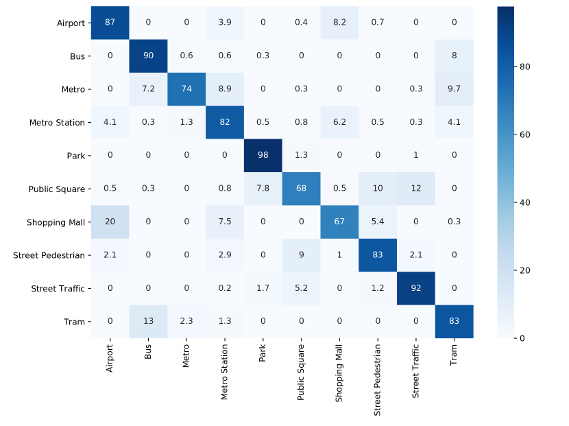
Figure 1: Confusion matrix result (Acc. %) obtained by PROD fusion of audio-CQT-Vgg14, audio-GAM-Vgg14, audio-MEL-Vgg14, and audio-emb-CNN14

TABLE VII: Performance comparison of visual-based frameworks

Visual-image	Acc.	Visual-embedding	Acc.
based models		based models
visual-image-Xception	85.9	visual-emb-Xception	80.3
visual-image-Vgg19	83.8	visual-emb-Vgg19	80.8
visual-image-Resnet50	86.3	visual-emb-Resnet50	82.0
visual-image-InceptionV3	88.9	visual-emb-InceptionV3	83.4
visual-image-MobileNetV2	84.4	visual-emb-MobileNetV2	80.2
visual-image-DenseNet121	87.8	visual-emb-DenseNet121	83.5
visual-image-NASNetLarge	86.9	visual-emb-NASNetLarge	81.5
MAX Fusion	90.2	MAX Fusion	86.5
MEAN Fusion	90.5	MEAN Fusion	81.8
PROD Fusion	91.1	PROD Fusion	84.3

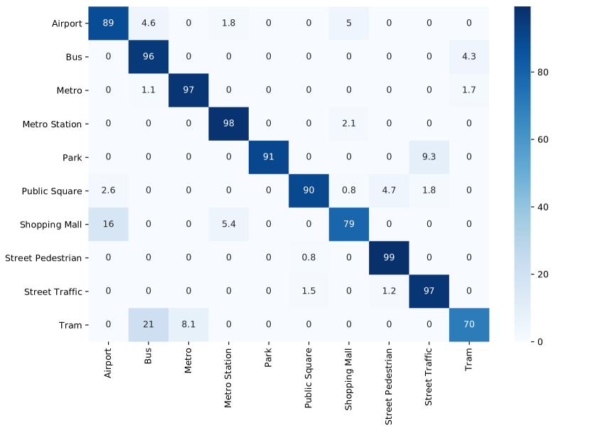
Figure 2: Confusion matrix result (Acc. %) obtained by PROD fusion of seven visual-image based frameworks

IV Experimental Results And Discussion

IV-A Analysis of audio-based deep learning frameworks for scene classification

As Table VI shows the accuracy results obtained from audio-based deep learning frameworks, we can see that all late fusion methods help to improve the performance significantly regarding both audio-spectrogram and audio-embedding approaches, achieving the highest score of 80.4% from PROD fusion of three audio-spectrogram based frameworks and 69.6% from MEAN fusion of five audio-embedding based frameworks. Compare the performance between two audio-based approaches proposed, it can be seen that directly training spectrogram inputs is more effective, achieving 68.3%, 69.6%, and 72.2% from CQT, GAM, and MEL spectrogram respectively, which outperform all results obtained from audio-emmbedding based frameworks. We further conduct PROD fusion of predicted probabilities obtained from three audio-spectrogram based frameworks (audio-CQT-Vgg14, audio-GAM-Vgg14, audio-MEL-Vgg14) and the audio-emb-CNN14 framework (the best framework in the audio-embedding based approach), achieving the classification accuracy of 82.2% with the confusion matrix shown in Fig. 1 and improving the DCASE baseline by 17.1% (Note that only audio data input is used for these frameworks and DCASE baseline). This proves that although the audio-embedding based approach shows low performance rather than the audio-spectrogram based approach, audio embeddings extracted from AudioSet dataset for AED task contain distinct features which is beneficial for SC task.

IV-B Analysis of visual-based deep learning frameworks for scene classification

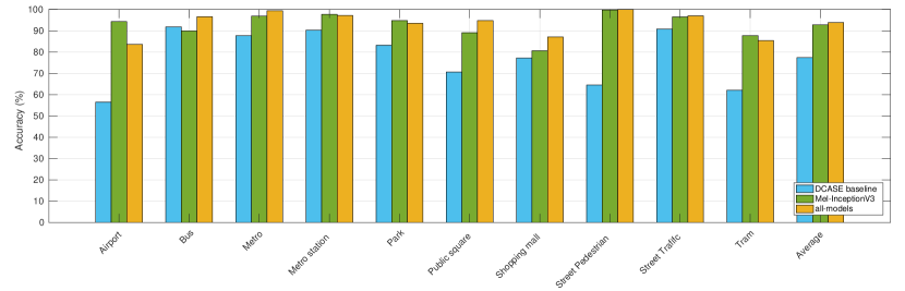
Figure 3: Performance comparison (Acc.%) of DCASE baseline, MEL-InceptionV3 and all-models across all scene categories

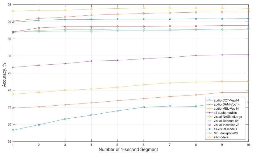
Figure 4: Performance of individual audio-spectrogram based frameworks (audio-CQT-Vgg14, audio-GAM-Vgg14, audio-MEL-Vgg14), PROD fusion of three audio-spectrogram based frameworks (all-audio-models), individual visual-image based frameworks (visual-image-NASNetLarnge, visual-image-Densnet121, visual-image-InceptionV3), PROD fusion of three visual-image based frameworks (all-visual-model), PROD fusion of audio-based and visual based frameworks (MEL-InceptionV3, all-models) with the increasing number of 1-second input segments

As obtained results are shown in Table VII, we can see that the visual-image based frameworks, which directly train image frame inputs, outperform visual-embedding based frameworks. While all late fusion methods over visual-image based frameworks help to improve the performance, only MAX fusion of image-embedding based frameworks shows to be effective. The PROD fusion of seven visual-image based frameworks achieves the best accuracy of 91.1%, improving DCASE baseline by 13.7% (Note that these frameworks and DCASE baseline only use visual data input). Comparing the performance between audio-based and visual-based approaches, the PROD fusion of seven visual-image based frameworks (91.1%) outperforms the best result of 82.2% from PROD fusion of audio-CQT-Vgg14, audio-GAM-Vgg14, audio-MEL-Vgg14, and audio-emb-CNN14 mentioned in Section IV-A. Further comparing the two confusion matrixes obtained from these two PROD fusions, as shown in Fig. 1 and Fig. 2, we can see that PROD fusion of seven visual-image based frameworks outperforms over almost scene categories except to ’Park’ and ’Tram’. As a result, we can conclude that visual data input contains more information for scene classification rather than audio data input.

IV-C Combine both visual and audio features for scene classification

As individual analysis of either audio or visual features within scene context classification is shown in Section IV-A and IV-B respectively, we can see that directly training and classifying audio/visual data input is more effective, rather than audio/image-embedding based approaches. We then evaluate a combination of audio and visual features by proposing two PROD fusions: (1) three audio-spectrogram based frameworks (audio-CQT-Vgg14, audio-GAM-Vgg14, audio-MEL-Vgg14) and top-3 visual-image frameworks (visual-image-DenseNet121, visual-image-InceptionV3, visual-image-NASNetLarge) referred to as all-models, and (2) one audio-spectroram based framework (audio-MEL-Vgg14) and one visual-image based framework (visual-image-InceptionV3) referred to as MEL-InceptionV3. As results shown in Fig. 3, all-models helps to achieve the highest accuracy classification score of 93.9%, improving DCASE baseline by 16.5% and showing improvement on all scene categories. Although MEL-InceptionV3 only fuses two frameworks, it achieves 92.8%, showing competitive to all-models fusing 6 frameworks. Notably, mis-classifying cases mainly occur among high cross-correlated categories in meta-class such as indoor (Airport, Metro station, and Shopping mall), outdoor (Park, Public square, Street pedestrian, and Street Traffic), and transportation (Bus, Metro, and Tram). If we aim to classify into three meta-classes (indoor, outdoor, and transportation), all-models helps to achieve a classification accuracy of 99.3%.

IV-D Early detecting scene context

We further evaluate whether deep learning frameworks can help to detect scene context early. To this end, we evaluate 10 different frameworks: (1-2-3) 3 individual audio-spectrogram based frameworks (audio-CQT-Vgg14, audio-GAM-Vgg14, audio-MEL-Vgg14), (4) PROD fusion of these three audio-spectrogram frameworks referred to as all-audio-models, (5-6-7) 3 visual-image based frameworks (visiual-image-NASNetLarge, visual-image-Densnet121, visual-image-InceptionV3), (8) PROD fusion of these three visual-image based frameworks referred to as all-visual-models, (9) MEL-InceptionV3, and (10) all-models. As the results shown in Fig. 4, while performance of audio-based frameworks is improved by time, visual-based frameworks are stable. As a result, when we combine audio and visual features, which are evaluated in MEL-InceptionV3 and all-models, the performance is improved by time and stable after 6 seconds. Notably, accuracy scores of both MEL-InceptionV3 and all-models are larger than 90.0% at the first second, which is potentially for real-life applications integrating the function of early detecting scene context.

V Conclusion

We conducted extensive experiments and explored various deep learning based frameworks for classifying 10 categories of urban scenes. Our method, which uses an ensemble of audio-based and visual-based frameworks, achieves the best classification accuracy of 93.9% on DCASE Task 1B development set. The obtained results outperform DCASE baseline, improving by 17.1% with only audio data input, 26.2% with only visual data input, and 16.5% with both audio-visual data. In further work, we will evaluate whether an end-to-end system using joint learning of audio-visual data input may help to improve the performance.

References

- [1] R. Arandjelović and Andrew Zisserman, “Objects that sound,” in ECCV, 2018.
- [2] Joon Son Chung, A. Senior, Oriol Vinyals, and Andrew Zisserman, “Lip reading sentences in the wild,” in IEEE Conference on Computer Vision and Pattern Recognition (CVPR), 2017, pp. 3444–3453.
- [3] Hang Zhao, Chuang Gan, Andrew Rouditchenko, Carl Vondrick, Josh H. McDermott, and A. Torralba, “The sound of pixels,” ArXiv, vol. abs/1804.03160, 2018.
- [4] Naoya Takahashi, Michael Gygli, and L. Van Gool, “Aenet: Learning deep audio features for video analysis,” IEEE Transactions on Multimedia, vol. 20, pp. 513–524, 2018.
- [5] C. Sanderson and B. Lovell, “Multi-region probabilistic histograms for robust and scalable identity inference,” in Proc. ICB, 2009.
- [6] Shiqing Zhang, Shiliang Zhang, Tiejun Huang, W. Gao, and Qi Tian, “Learning affective features with a hybrid deep model for audio–visual emotion recognition,” IEEE Transactions on Circuits and Systems for Video Technology, vol. 28, pp. 3030–3043, 2018.
- [7] Ruohan Gao, Tae-Hyun Oh, K. Grauman, and L. Torresani, “Listen to look: Action recognition by previewing audio,” in IEEE/CVF Conference on Computer Vision and Pattern Recognition (CVPR), 2020, pp. 10454–10464.
- [8] Fabian Caba Heilbron, Victor Escorcia, Bernard Ghanem, and Juan Carlos Niebles, “Activitynet: A large-scale video benchmark for human activity understanding,” in IEEE Conference on Computer Vision and Pattern Recognition (CVPR), 2015, pp. 961–970.
- [9] K. Soomro, A. Zamir, and M. Shah, “Ucf101: A dataset of 101 human actions classes from videos in the wild,” ArXiv, vol. abs/1212.0402, 2012.
- [10] Rikke Gade, Mohamed Abou-Zleikha, M. G. Christensen, and T. Moeslund, “Audio-visual classification of sports types,” in IEEE International Conference on Computer Vision Workshop (ICCVW), 2015, pp. 768–773.
- [11] A. Karpathy, G. Toderici, Sanketh Shetty, Thomas Leung, R. Sukthankar, and Li Fei-Fei, “Large-scale video classification with convolutional neural networks,” in IEEE Conference on Computer Vision and Pattern Recognition, 2014, pp. 1725–1732.
- [12] Detection and Classification of Acoustic Scenes and Events Community, DCASE 2021 challenges, http://dcase.community/challenge2021.
- [13] Shanshan Wang, Annamaria Mesaros, Toni Heittola, and Tuomas Virtanen, “A curated dataset of urban scenes for audio-visual scene analysis,” arXiv preprint arXiv:2011.00030, 2020.
- [14] L. Pham, I. Mcloughlin, Huy Phan, R. Palaniappan, and A. Mertins, “Deep feature embedding and hierarchical classification for audio scene classification,” in International Joint Conference on Neural Networks (IJCNN), 2020, pp. 1–7.
- [15] L. Pham, Huy Phan, T. Nguyen, R. Palaniappan, A. Mertins, and I. Mcloughlin, “Robust acoustic scene classification using a multi-spectrogram encoder-decoder framework,” Digital Signal Processing, vol. 110, pp. 102943, 2021.
- [16] L. Pham, I. McLoughlin, H. Phan, R. Palaniappan, and Y. Lang, “Bag-of-features models based on C-DNN network for acoustic scene classification,” in Proc. AES, 2019.
- [17] Lam Pham, Ian Mcloughlin, Huy Phan, and Ramaswamy Palaniappan, “A robust framework for acoustic scene classification,” in Proc. INTERSPEECH, 2019, pp. 3634–3638.
- [18] D. Ngo, Hao Hoang, A. Nguyen, Tien Ly, and L. Pham, “Sound context classification basing on join learning model and multi-spectrogram features,” ArXiv, vol. abs/2005.12779, 2020.
- [19] Truc Nguyen and Franz Pernkopf, “Acoustic scene classification using a convolutional neural network ensemble and nearest neighbor filters,” in Proc. DCASE, 2018, pp. 34–38.
- [20] Brian McFee, Raffel Colin, Liang Dawen, D.P.W. Ellis, McVicar Matt, Battenberg Eric, and Nieto Oriol, “librosa: Audio and music signal analysis in python,” in Proceedings of The 14th Python in Science Conference, 2015, pp. 18–25.
- [21] D P W (2009) Ellis, “Gammatone-like spectrogram,” 2009.
- [22] Kele Xu, Dawei Feng, Haibo Mi, Boqing Zhu, Dezhi Wang, Lilun Zhang, Hengxing Cai, and Shuwen Liu, “Mixup-based acoustic scene classification using multi-channel convolutional neural network,” in Pacific Rim Conference on Multimedia, 2018, pp. 14–23.
- [23] Yuji Tokozume, Yoshitaka Ushiku, and Tatsuya Harada, “Learning from between-class examples for deep sound recognition,” in ICLR, 2018.
- [24] Sergey Ioffe and Christian Szegedy, “Batch normalization: Accelerating deep network training by reducing internal covariate shift,” in Proceedings of the 32nd International Conference on Machine Learning, 2015, pp. 448–456.
- [25] Vinod Nair and Geoffrey E Hinton, “Rectified linear units improve restricted boltzmann machines,” in ICML, 2010.
- [26] Nitish Srivastava, Geoffrey Hinton, Alex Krizhevsky, Ilya Sutskever, and Ruslan Salakhutdinov, “Dropout: a simple way to prevent neural networks from overfitting,” The Journal of Machine Learning Research, vol. 15, no. 1, pp. 1929–1958, 2014.
- [27] Karen Simonyan and Andrew Zisserman, “Very deep convolutional networks for large-scale image recognition,” in International Conference on Learning Representations, 2015.
- [28] Q. Kong, Y. Cao, T. Iqbal, Y. Wang, W. Wang, and M. D. Plumbley, “Panns: Large-scale pretrained audio neural networks for audio pattern recognition,” IEEE/ACM Transactions on Audio, Speech, and Language Processing, vol. 28, pp. 2880–2894, 2020.
- [29] Jort F. Gemmeke, Daniel P. W. Ellis, Dylan Freedman, Aren Jansen, Wade Lawrence, R. Channing Moore, Manoj Plakal, and Marvin Ritter, “Audio set: An ontology and human-labeled dataset for audio events,” in Proc. ICASSP, 2017.
- [30] François Chollet et al., “Keras,” https://keras.io, 2015.
- [31] Olga Russakovsky, Jia Deng, Hao Su, Jonathan Krause, Sanjeev Satheesh, Sean Ma, Zhiheng Huang, Andrej Karpathy, Aditya Khosla, Michael Bernstein, Alexander C. Berg, and Li Fei-Fei, “ImageNet Large Scale Visual Recognition Challenge,” International Journal of Computer Vision (IJCV), vol. 115, no. 3, pp. 211–252, 2015.
- [32] Solomon Kullback and Richard A Leibler, “On information and sufficiency,” The annals of mathematical statistics, vol. 22, no. 1, pp. 79–86, 1951.
- [33] Diederik P. Kingma and Jimmy Ba, “Adam: A method for stochastic optimization,” CoRR, vol. abs/1412.6980, 2015.