A Low-Compexity Deep Learning Framework
For Acoustic Scene Classification

Abstract

In this paper, we presents a low-complexity deep learning frameworks for acoustic scene classification (ASC). The proposed framework can be separated into three main steps: Front-end spectrogram extraction, back-end classification, and late fusion of predicted probabilities. First, we use Mel filter, Gammatone filter and Constant Q Transfrom (CQT) to transform raw audio signal into spectrograms, where both frequency and temporal features are presented. Three spectrograms are then fed into three individual back-end convolutional neural networks (CNNs), classifying into ten urban scenes. Finally, a late fusion of three predicted probabilities obtained from three CNNs is conducted to achieve the final classification result. To reduce the complexity of our proposed CNN network, we apply two model compression techniques: model restriction and decomposed convolution. Our extensive experiments, which are conducted on DCASE 2021 (IEEE AASP Challenge on Detection and Classification of Acoustic Scenes and Events) Task 1A development dataset, achieve a low-complexity CNN based framework with 128 KB trainable parameters and the best classification accuracy of 66.7%, improving DCASE baseline by 19.0%.

Key words— Convlutional neural network, Gammatone filter, constant Q transoform, MEL filter, spectrogram, deep learning.

I Introduction

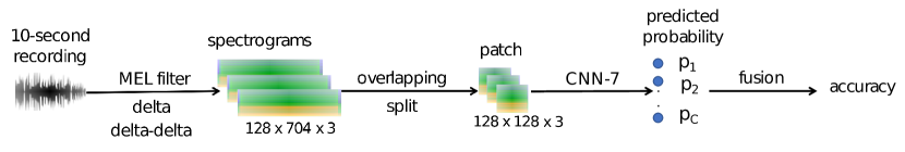
Figure 1: High-level architecture of ASC baseline system proposed.

TABLE I: The CNN-7 network architecture baseline (input patch of $128{\times}128{\times}3$)

Network architecture	Output
BN - Convolution ([$3{\times}3]$@$C_{out}1=32$) - ReLU - BN - Dropout (10%)	$128{\times}128{\times}32$
BN - Convolution ([$3{\times}3]$@$C_{out}2=32$) - ReLU - BN - AP [$2{\times}2$] - Dropout (10%)	$64{\times}64{\times}32$
BN - Convolution ([$3{\times}3]$@$C_{out}3=64$) - ReLU - BN - Dropout (10%)	$64{\times}64{\times}64$
BN - Convolution ([$3{\times}3]$@$C_{out}4=64$) - ReLU - BN - AP [$2{\times}2$] - Dropout (10%)	$32{\times}32{\times}64$
BN - Convolution ([$3{\times}3]$@$C_{out}5=128$) - ReLU - BN - AP [$2{\times}2$] - Dropout (10%)	$16{\times}16{\times}128$
BN - Convolution ([$3{\times}3]$@$C_{out}6=128$) - ReLU - BN - GAP - Dropout (10%)	$128$
FC - Softmax	$C=10$

Acoustic Scene Classification (ASC), one of main research fields of ‘Machine Hearing’ [1], has drawn much attention in recent years and has been applied to a wide range of real-life applications such as enhancing the listening experience of users by detecting scene context [2, 3], supporting sound event detection [4] or integrating in a multiple-sensor automatic system [5]. To deal with ASC challenges such as unbalanced data, lacking data input, or mismatch recording devices, various methods have been proposed, which can be separated into two main approaches. The first approach makes use of multiple data input such as ensemble of spectrograms [6, 7, 8] or audio channels [9]. Meanwhile, the second approach focuses on back-end classification, and proposes powerful deep learning network architectures, which are able to enforce the training process [10, 11, 12, 13]. Although these two approaches can achieve good results, they present high-complexity systems. Indeed, while multiple input data requires an ensemble of multiple individual classification models [14, 15], powerful network architectures show a number of convolutional layers [10, 11]. All top-10 systems proposed in recent DCASE chalenges in 2018, 2019, 2020 are also based on complex architectures, requiring larger than 2 MB of trainable parameters. This issue of network complexity prevents implementing edge devices concerning real-life applications which require a low footprint. Although there are various methods proposed to deal with the issue of model complexity such as quantizaton [16], pruning [17, 18], model restriction (i.e. restriction on the number of layers [19], the number of kernel [20], or both of these factors [21]), decomposed convolution [22], hybrid methods using pruning and decomposed convolution [22], pruning and distillation [23], these are mainly applied for image data. Therefore, our work introduces a low-complexity deep learning framework for ASC. To deal with ASC challenges, we propose an ensemble of multiple spectrogram inputs, using Mel filter [24], Gammaton [25] filter, and CQT [24]. For each network used for training an individual spectrogram input, we deal with the issue of model complexity by combining model restriction and decomposed convolution methods.

The remaining of our paper is organized as follows: Section 2 presents deep learning frameworks proposed and model compression techniques. Section 3 introduces evaluation setup where experimental setting, metric, and implementation of deep learning frameworks proposed are presented. Next, Section 4 presents and analyses the experimental results. Finally, Section 5 presents conclusion and future work.

II The low-complexity deep learning framework proposed

II-A Our baseline

We first propose a baseline with a high-level architecture shown in Fig. 1, which comprises three main steps in the order of front-end spectrogram feature extraction, back-end classification, and a fusion of predicted probabilities. In the first step, a raw audio signal is firstly transformed into a spectrogram of $129\times 704$ by using MEL filter [24] with Fast Fourier Transform (FFT) number, window size, and hope size set to 8192, 4096, and 620, respectively. As delta and delta-delta across the temporal dimension are applied to the spectrogram, we then generate the spetrograms of $129\times 704\times 3$. Next, the spectrograms are split into 10 patches of $128\times 128\times 3$ with 50% overlapping before feeding into a CNN based network for classification.

As we illustrate our proposed CNN based network architecture in Table I, it contains sub-blocks, which perform convolution with $C_{out}$ channel (Convolution ([kernel size]$@C_{out}$)), batch normalization (BN) [26], rectified linear units (ReLU) [27], average pooling (AV [kernel size]), global average pooling (GAP), dropout (percentage dropped) [28], fully-connected (FC), and Softmax layers. The dimension of Softmax layer is set to $C=10$ that equals to the number of scene context classified. In total, we have 6 convolutional layers and 1 fully-connected layers that makes the proposed network architecture like CNN-7.

As the CNN-7 works on patches, the final predicted probability of an entire spectrogram is computed by averaging of all patches. Let us consider $\mathbf{P^{n}}=(\mathbf{p_{1}^{n},p_{2}^{n},...,p_{C}^{n}})$, with $C$ being the category number and the $n^{th}$ out of $N$ patches fed into the CNN-7, as the probability of a test instance, then the average classification probability is denoted as $\mathbf{\bar{p}}=(\bar{p}_{1},\bar{p}_{2},...,\bar{p}_{C})$ where,

$$\bar{p}_{c}=\frac{1}{N}\sum_{n=1}^{N}p_{c}^{n}~{}~{}~{}for~{}~{}1\leq n\leq N$$ (1)

and the predicted label $\hat{y}$ of the test instance evaluated is determined as:

$$\hat{y}=argmax(\bar{p}_{1},\bar{p}_{2},...,\bar{p}_{C})$$ (2)

II-B Ensemble of multiple spectrogram inputs

Although both of CQT and STFT spectrograms are built on Fourier Transform theory, they extract different central frequencies. Meanwhile, both Mel spectrogram and Gammatongram are generated from STFT spectrogram, but use two different filter banks: Mel and Gammatone filters. We can conclude that three spectrograms either extract different central frequencies or apply different auditory models. Therefore, each spectrogram may contain its own distinct and complimentary information. This inspires us to propose an ensemble of these three spectrograms as a rule of thumb to improve the ASC performance [14, 15]. To evaluate the ensemble of multiple spectrograms, we proposed a late fusion scheme, referred to as PROD fusion. In particular, we conduct experiments over individual networks with different spectrogram inputs, then obtain predicted probability of each network as $\mathbf{\bar{p_{s}}}=(\bar{p}_{s1},\bar{p}_{s2},...,\bar{p}_{sC})$, where $C$ is the category number and the $s^{th}$ out of $S$ networks evaluated. Next, the predicted probability after PROD fusion $\mathbf{p_{f-prod}}=(\bar{p}_{1},\bar{p}_{2},...,\bar{p}_{C})$ is obtained by:

$$\bar{p_{c}}=\frac{1}{S}\prod_{s=1}^{S}\bar{p}_{sc}~{}~{}~{}for~{}~{}1\leq s\leq S$$ (3)

Finally, the predicted label $\hat{y}$ is determined by (2).

II-C Model compression methods applied to the CNN-7 network

Our proposed CNN-7 architecture reports a complexity of 1,129 MB for non-zero parameters with using 32 bits for representing one trainable parameter. Additionally, using ensemble of three spectrogram inputs make the number of trainable parameters further increase three times. To reduce the model complexity, we firstly restrict the number of channels used in the CNN-7 baseline, then reduce the channels of $C_{out}1$ from 32 to 16, $C_{out}3$ and $C_{out}4$ from 64 to 32, $C_{out}5$ and $C_{out}6$ from 128 to 64. Our proposed channel restriction (CR) helps to reduce an individual CNN-7 complexity to 313 KB that nearly equals to 1/4 of the original size.

We further reduce the CNN-7 complexity by applying the decomposed convolution (DC) technique described in [22, 29]. Let us consider $C_{in}$ and $C_{cout}$ as the input and output channel numbers respectively, $W=3$ and $L=3$ are the dimensions of kernel size, which are used for a convolutional layer. Then, the number of trainable parameters at a convolutional layer is computed by $W\times L\times C_{in}\times C_{out}=9\times C_{in}\times C_{out}$ . We reduce the number of trainable parameters at a convolutional layer by decomposing the convolutional layer into 4 sub-convolutional layers as described in Fig. 2. For all four sub-convolutional layers, the output channel is reduced to $C_{out}/4$. Regarding the first sub-convolutional layer (the upper path shown in Fig. 2), although we still use kernel size of [W$\times$L]=[3$\times$3], we reduce the input channels to $C_{in}$/4, then cost $(9\times C_{in}\times C_{out})/16$ trainable parameters. Regarding the other sub-convolution layers, we reduce the kernel size to [W$\times$L]=[1$\times$1]. While the second and third sub-convolutional layers (two middle paths shown in Fig. 2), the input channel is reduced to $C_{in}/2$, it is remained in the fourth sub-convolutional layer (the lower path shown in Fig. 2). As a result, it requires $(C_{in}\times C_{out})/8$ for the second and third sub-convolutional layers, and $(C_{in}\times C_{out})/4$ for the fourth sub-convolution layer. By decomposing a convolutional layer into four sub-convolutional layers, the model complexity is reduced to nearly 1/8.5 of the original size. By combining the two model compression techniques, we can achieve a CNN-7 network architecture with complexity of 42.6 KB, which nearly equals to 1/25 of the original size (i.e. the original CNN-7 network architecture is proposed in the baseline framework in Table I). As we need to use three CNN-7 for three different spectrogram inputs, the final complexity of the proposed framework is approximately 128 KB.

III Evaluation Setting

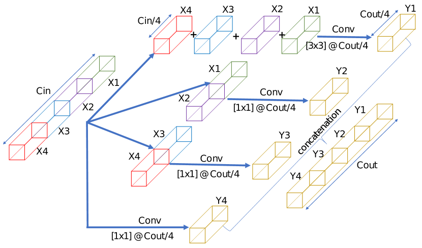
Figure 2: Decomposed convolution technique applied to a convolutional layer.

III-A TAU Urban Acoustic Scenes 2020 Mobile, development dataset [30] (DCASE 2021 Task 1A)

This dataset was proposed for DCASE 2021 challenge [31], which requires a limitation of model complexity set to 128 KB with using 32 bits for one trainable parameter. The dataset in slightly unbalanced, recorded from 12 large European cities: Amsterdam, Barcelona, Helsinki, Lisbon, London, Lyon, Madrid, Milan, Prague, Paris, Stockholm, and Vienna. It consists of 10 scene classes: airport, shopping mall (indoor), metro station (underground), pedestrian street, public square, street (traffic), traveling by tram, bus and metro (underground), and urban park. The audio recordings were recorded from 3 different devices namely A (10215 recordings), B (749 recordings), C (748 recordings). Additionally, synthetic data for 11 mobile devices was created based on the original recordings, referred to as S1 (750 recordings), S2 (750 recordings), S3 (750 recordings), S4 (750 recordings), S5 (750 recordings), and S6 (750 recordings).

As a result, this task not only requires low complexity model, but it also proposes an issue of mismatch recording devices. To evaluate, we follow the DCASE 2021 Task 1A challenge [31], separate this dataset into training (Train.) and evaluation (Eval.) subsets as shown in Table II. Then, Train. subset is used for training frameworks proposed and Eval. subset is used for evaluating. Notably, two of 12 cities and S4, S5, S6 audio recordings are only presented in the Eval. subset for evaluating the issue of mismatch recording devices and unseen samples.

III-B Deep learning framework implementation

We use Tensorflow framework to build all classification models in this papers. The cross-entropy loss function used for training is described as

$$LOSS_{EN}(\Theta)=-\frac{1}{N}\sum_{n=1}^{N}\mathbf{y_{n}}\log\left\{\mathbf{\hat{y}_{n}}(\Theta)\right\}$$ (4)

defined over all parameters $\Theta$, and $N$ is the number of training samples. $\mathbf{y_{n}}$ and $\mathbf{\hat{y}_{n}}$ denote ground truth and predicted output. The training is carried out for 100 epochs using Adam  [32] for optimization.

III-C Metric for evaluation

TABLE II: The number of 10-second audio-visual scene recordings corresponding to each scene categories in the Train. and Eval. subsets separated from the DCASE 2021 Task 1A development dataset [33].

Category	Train.	Eval.
Airport	1393	296
Bus	1400	297
Metro	1382	297
Metro Station	1380	297
Park	1429	297
Public square	1427	297
Shopping mall	1373	297
Street pedestrian	1386	297
Street traffic	1413	297
Tram	1379	296
Total	13962	2968
	($\approx$38.79 hours)	($\approx$8.25 hours)

Regarding the evaluation metric used in this paper, we follow DCASE 2021 challenge. Let us consider $C$ as the number of audio/visual test samples which are correctly classified, and the total number of audio/visual test samples is $T$, the classification accuracy (Acc. (%)) is the % ratio of $C$ to $T$.

III-D Optimize the framework proposed by evaluating factors of time length and data augmentation

TABLE III: Performance comparison among three spectrograms with different time lengths, with or without using data augmentation

	Without data augmentation				Data augmentation
Spectrogram	1-second	2-second	5-second	10-second	1-second	2-second	5-second	10-second
MEL	56.7	57.9	56.2	60.5	54.6	57.9	59.5	58.4
GAM	53.2	55.0	53.1	53.9	58.9	60.1	60.6	57.1
CQT	44.3	47.7	48.6	49.2	44.2	45.7	48.6	49.1

TABLE IV: Performance comparison among DCASE baseline, the CNN-7 baseline, the CNN-7 baseline with channel restriction (CNN-7 w/ CR), the CNN-7 baseline with channel restriction and decomposed convolution (CNN-7 w/ CR & DC).

	DCASE	CNN-7	CNN-7	CNN-7 w/
	baseline	baseline	w/ CR	CR & DC
Category	(90.3 KB)	(1.1 MB)	(313 KB)	(42.6 KB)
Airport	40.5	59.5	50.3	64.5
Bus	47.1	73.7	70.4	69.0
Metro	51.9	57.6	49.8	70.0
Metro station	28.3	53.9	48.1	45.1
Park	69.0	73.1	78.5	74.4
Public square	25.3	34.3	38.4	25.9
Shopping mall	61.3	52.9	50.2	43.4
Street pedestrian	38.7	39.4	35.0	32.7
Street traffic	62.0	84.5	88.2	89.6
Tram	53.0	67.9	62.5	52.7
Average	47.7	59.7	57.1	56.7

In this paper, we further evaluate factors of time length and data augmentation which may affect the ASC performance, then find the most optimized framework. In particular, we evaluate four different time lengths of 1 second (i.e. 1-second patch is used in the baseline proposed), 2 seconds, 5 seconds and 10 seconds (entire audio recording). In order to evaluate different time lengths mentioned but still keep the input patch of 128$\times$128$\times$3 unchanged, the hop size is set to 620, 1120, 1850 for 1-second, 2-second, and 5-second lengths respectively, while the other setting mentioned in Section II-A are unchanged. To evaluate an entire 10-second recording, the hop size is set to 2048, then generate one patch of 128$\times$200$\times$3.

We enforce the back-end classifiers by applying two methods of data augmentation on the patches: mixup [34, 35], and spectrum agumentation [36]. We then compare the ASC performance with and without using these data augmentation methods. As we apply mixup data augmentation [34, 35], the labels of the mixup data input are no longer one-hot. We therefore train back-end classifiers with Kullback-Leibler (KL) divergence loss [37] rather than the standard cross-entropy loss over all $N$ mixup training samples:

$$LOSS_{KL}(\Theta)=\sum_{n=1}^{N}\mathbf{y}_{n}\log(\frac{\mathbf{y}_{n}}{\mathbf{\hat{y}}_{n}})+\frac{\lambda}{2}||\Theta||_{2}^{2},$$ (5)

where $\Theta$ denotes the trainable network parameters and $\lambda$ denote the $\ell_{2}$-norm regularization coefficient. $\mathbf{y_{c}}$ and $\mathbf{\hat{y}_{c}}$ denote the ground-truth and the network output, respectively. The training is carried out for 100 epochs using Adam [32] for optimization.

IV Experimental Results And Discussion

IV-A Performance comparison between DCASE baseline and the CNN-7 baseline with or without using model compression methods

As experimental results are shown in Table IV, although the CNN-7 baseline outperforms DCASE baseline and helps to improve the accuracy by 12%, the CNN-7 baseline complexity is much larger than DCASE baseline. By using model compression methods, we can achieve a low-complexity model referred to as CNN-7 with CR & DC, which is nearly 1/2 of the DCASE baseline complexity, but still outperforms DCASE baseline showing an accuracy improvement of 9%.

IV-B Effect of time length, data augmentation, spectrogram input

Next, we conduct experiments to evaluate effect of spectrogram input, time length, and data augmentation on the CNN-7 with CR & DC, which are shown in Table III. As experimental results are shown in Table III, MEL and GAM outperform CQT at different time lengths and with or without using data augmentation. Without using data augmentation, MEL obtains better results than GAM at different time lengths. However, both MEL and GAM achieve competitive results with using data augmentation. It can be seen that data augmentation is effective only for GAM. Additionally, increasing time length helps to improve the accuracy for both CQT and MEL, but not much effective for GAM. As a result, we finally configure an optimized and low-complexity framework for ASC task with setting: CNN-7 with CR & DC, 5-second time length, and using mixup & spectrum data augmentation.

IV-C Evaluate ensemble of different spectrogram inputs

Given the optimized framework, we conduct PROD fusion of three predicted probabilities from three spectrogram inputs (i.e. PROD fusion is mentioned in Section II-B) to obtain the final classification accuracy. We then compare performances among DCASE baseline, the optimized framework with individual spectrograms, the optimized framework with the ensemble of multiple spectrograms, across all scene categories. As experimental results are shown in Fig.3, GAM and MEL achieve competitive results, and outperform CQT at almost scene categories except for ’Airport’ and ’Bus’. The ensemble of three spectrogram inputs helps to achieve an average accuracy of 66.7%, improving DCASE baseline by 19.0%, and notably showing improvement over all scene categories.

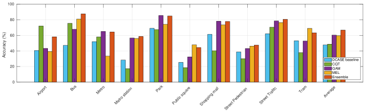
Figure 3: Performance comparison (Acc.%) of DCASE baseline, individual spectrograms (CQT, GAM, and MEL), and the ensemble of three spectrograms across all scene categories (using CNN-7 with CR & DC, 5-second time length, and mixup & spectrum data augmentation for each spectrogram input)

Further analysing performance over different recording devices as shown in Table V, we see that device A outperforms the other devices as this device is dominant in Train. subset. Although there is a lacking of training samples for device B and C, they achieves competitive accuracy of 69.6% and 70.8% respectively, compared with device A performance of 79.1%. Regarding synthesized devices from S1 to S6, although there is no samples from S4, S5, S6 in Train. subset, the performance of these devices are competitive to the other S1, S2, S3. Our results and analysis indicate that the ASC framework proposed not only shows low complexity of 128 KB, it also can tackle the issue of mismatched recording devices.

V Conclusion

We have just presented a low-complexity framework for ASC, which makes use of multiple spectrogram inputs and model compression techniques. While the ensemble of multiple spectrograms helps to tackle different ASC challenges of mismatch recording devices or lacking input to improve the ASC performance, a combination of model restriction and decomposed convolution techniques is effective to achieve a low model complexity of 128 KB. In the future, we will further compress the model complexity by combining our proposed approaches with other techniques of distillation, pruning, and quantization.

TABLE V: The number of 10-second audio-visual scene recordings corresponding to each device in the Train. and Eval. subsets separated from the DCASE 2021 Task 1A development dataset [33] and performance for each devices.

Devices	Train.	Eval.	Acc. %
A	10215	330	79.1
B	749	329	69.6
C	748	329	70.8
S1	750	330	65.8
S2	750	330	63.6
S3	750	330	67.0
S4	0	330	63.9
S5	0	330	60.0
S6	0	330	60.3

References

- [1] Richard F. Lyon, Human and Machine Hearing, Cambridge University Press, 2017.
- [2] S. Ravindran and D.V. Anderson, “Audio classification and scene recognition and for hearing aids,” in IEEE International Symposium on Circuits and Systems, 2005, pp. 860–863.
- [3] JuanJuan Xiang, Martin F. McKinney, Kelly Fitz, and Tao Zhang, “Evaluation of sound classification algorithms for hearing aid applications,” in IEEE International Conference on Acoustics, Speech and Signal Processing, 2010, pp. 185–188.
- [4] Damiano Oldoni, Bert De Coensel, Michaël Rademaker, Bernard De Baets, and Dick Botteldooren, “Context-dependent environmental sound monitoring using som coupled with legion,” in The International Joint Conference on Neural Networks (IJCNN), 2010, pp. 1–8.
- [5] Liping Yang, Xinxing Chen, and Lianjie Tao, “Acoustic scene classification using multi-scale features,” in Proc. DCASE, 2018, pp. 29–33.
- [6] L. Pham, I. Mcloughlin, Huy Phan, R. Palaniappan, and A. Mertins, “Deep feature embedding and hierarchical classification for audio scene classification,” in International Joint Conference on Neural Networks (IJCNN), 2020, pp. 1–7.
- [7] D. Ngo, Hao Hoang, A. Nguyen, Tien Ly, and L. Pham, “Sound context classification basing on join learning model and multi-spectrogram features,” ArXiv, vol. abs/2005.12779, 2020.
- [8] Truc Nguyen and Franz Pernkopf, “Acoustic scene classification using a convolutional neural network ensemble and nearest neighbor filters,” in Proc. DCASE, 2018, pp. 34–38.
- [9] Yuma Sakashita and Masaki Aono, “Acoustic scene classification by ensemble of spectrograms based on adaptive temporal divisions,” Tech. Rep., DCASE Challenge, 2018.
- [10] L. Pham, Huy Phan, T. Nguyen, R. Palaniappan, A. Mertins, and I. Mcloughlin, “Robust acoustic scene classification using a multi-spectrogram encoder-decoder framework,” Digital Signal Processing, vol. 110, pp. 102943, 2021.
- [11] Sai Phaye, Emmanouil Benetos, and Ye Wang, “SubSpectralNet using sub-spectrogram based convolutional neural networks for acoustic scene classification,” in Proc. ICASSP, 2019, pp. 825–829.
- [12] Zhao Ren, Kun Qian, Yebin Wang, Zixing Zhang, Vedhas Pandit, Alice Baird, and Bjorn Schuller, “Deep scalogram representations for acoustic scene classification,” IEEE/CAA Journal of Automatica Sinica, vol. 5, no. 3, pp. 662–669, 2018.
- [13] Hongwei Song, Jiqing Han, Shiwen Deng, and Zhihao Du, “Acoustic scene classification by implicitly identifying distinct sound events,” in Proc. INTERSPEECH, 2019, pp. 3860–3864.
- [14] L. Pham, I. McLoughlin, H. Phan, R. Palaniappan, and Y. Lang, “Bag-of-features models based on C-DNN network for acoustic scene classification,” in Proc. AES, 2019.
- [15] Lam Pham, Ian Mcloughlin, Huy Phan, and Ramaswamy Palaniappan, “A robust framework for acoustic scene classification,” in Proc. INTERSPEECH, 2019, pp. 3634–3638.
- [16] Vivienne Sze, Yu-Hsin Chen, Tien-Ju Yang, and Joel S Emer, “Efficient processing of deep neural networks: A tutorial and survey,” Proceedings of the IEEE, vol. 105, no. 12, pp. 2295–2329, 2017.
- [17] Song Han, Jeff Pool, John Tran, and William J Dally, “Learning both weights and connections for efficient neural networks,” arXiv preprint arXiv:1506.02626, 2015.
- [18] Jonathan Frankle and Michael Carbin, “The lottery ticket hypothesis: Finding sparse, trainable neural networks,” arXiv preprint arXiv:1803.03635, 2018.
- [19] Kaiming He, Xiangyu Zhang, Shaoqing Ren, and Jian Sun, “Deep residual learning for image recognition,” in Proceedings of the IEEE conference on computer vision and pattern recognition, 2016, pp. 770–778.
- [20] Sergey Zagoruyko and Nikos Komodakis, “Wide residual networks,” arXiv preprint arXiv:1605.07146, 2016.
- [21] Mingxing Tan and Quoc Le, “Efficientnet: Rethinking model scaling for convolutional neural networks,” in International Conference on Machine Learning. PMLR, 2019, pp. 6105–6114.
- [22] Yong-Deok Kim, Eunhyeok Park, Sungjoo Yoo, Taelim Choi, Lu Yang, and Dongjun Shin, “Compression of deep convolutional neural networks for fast and low power mobile applications,” arXiv preprint arXiv:1511.06530, 2015.
- [23] Vinu Joseph, Shoaib Ahmed Siddiqui, Aditya Bhaskara, Ganesh Gopalakrishnan, Saurav Muralidharan, Michael Garland, Sheraz Ahmed, and Andreas Dengel, “Reliable model compression via label-preservation-aware loss functions,” arXiv preprint arXiv:2012.01604, 2020.
- [24] Brian McFee, Raffel Colin, Liang Dawen, D.P.W. Ellis, McVicar Matt, Battenberg Eric, and Nieto Oriol, “librosa: Audio and music signal analysis in python,” in Proceedings of The 14th Python in Science Conference, 2015, pp. 18–25.
- [25] D P W (2009) Ellis, “Gammatone-like spectrogram,” 2009.
- [26] Sergey Ioffe and Christian Szegedy, “Batch normalization: Accelerating deep network training by reducing internal covariate shift,” in Proceedings of the 32nd International Conference on Machine Learning, 2015, pp. 448–456.
- [27] Vinod Nair and Geoffrey E Hinton, “Rectified linear units improve restricted boltzmann machines,” in ICML, 2010.
- [28] Nitish Srivastava, Geoffrey Hinton, Alex Krizhevsky, Ilya Sutskever, and Ruslan Salakhutdinov, “Dropout: a simple way to prevent neural networks from overfitting,” The Journal of Machine Learning Research, vol. 15, no. 1, pp. 1929–1958, 2014.
- [29] Khaled Koutini, Florian Henkel, Hamid Eghbal-zadeh, and Gerhard Widmer, “Low-complexity models for acoustic scene classification based on receptive field regularization and frequency damping,” arXiv preprint arXiv:2011.02955, 2020.
- [30] Annamaria Mesaros, Toni Heittola, and Tuomas Virtanen, “A multi-device dataset for urban acoustic scene classification,” in Proceedings of the Detection and Classification of Acoustic Scenes and Events (DCASE), 2018, pp. 9–13.
- [31] Detection and Classification of Acoustic Scenes and Events Community, DCASE 2021 challenges, http://dcase.community/challenge2021.
- [32] Diederik P. Kingma and Jimmy Ba, “Adam: A method for stochastic optimization,” CoRR, vol. abs/1412.6980, 2015.
- [33] Shanshan Wang, Annamaria Mesaros, Toni Heittola, and Tuomas Virtanen, “A curated dataset of urban scenes for audio-visual scene analysis,” arXiv preprint arXiv:2011.00030, 2020.
- [34] Kele Xu, Dawei Feng, Haibo Mi, Boqing Zhu, Dezhi Wang, Lilun Zhang, Hengxing Cai, and Shuwen Liu, “Mixup-based acoustic scene classification using multi-channel convolutional neural network,” in Pacific Rim Conference on Multimedia, 2018, pp. 14–23.
- [35] Yuji Tokozume, Yoshitaka Ushiku, and Tatsuya Harada, “Learning from between-class examples for deep sound recognition,” in ICLR, 2018.
- [36] Daniel S Park, William Chan, Yu Zhang, Chung-Cheng Chiu, Barret Zoph, Ekin D Cubuk, and Quoc V Le, “Specaugment: A simple data augmentation method for automatic speech recognition,” arXiv preprint arXiv:1904.08779, 2019.
- [37] Solomon Kullback and Richard A Leibler, “On information and sufficiency,” The annals of mathematical statistics, vol. 22, no. 1, pp. 79–86, 1951.