LENAS: Learning-based Neural Architecture Search and Ensemble for 3D Radiotherapy Dose Prediction

Abstract

Radiation therapy treatment planning is a complex process, as the target dose prescription and normal tissue sparing are conflicting objectives. In order to reduce human planning time efforts and improve the quality of treatment planning, knowledge-based planning (KBP) is in high demand. In this study, we propose a novel learning based ensemble approach, named LENAS, which integrates neural architecture search (NAS) with knowledge distillation for 3D radiotherapy dose prediction. Specifically, the prediction network first exhaustively searches each block from an enormous architecture space. Then, multiple architectures with promising performance and a large diversity are selected. To reduce the inference time, we adopt the teacher-student paradigm by treating the combination of diverse outputs from multiple learned networks as supervisions to guide the student network training. In addition, we apply adversarial learning to optimize the student network to recover the knowledge in teacher networks. To the best of our knowledge, this is the first attempt to investigate NAS and knowledge distillation in ensemble learning, especially in the field of medical image analysis. The proposed method has been evaluated on two public datasets, i.e., the OpenKBP and AIMIS dataset. Extensive experimental results demonstrate the effectiveness of our method and its superior performance to the state-of-the-art methods. In addition, several in-depth analysis and empirical guidelines are derived for ensemble learning.

I Introduction

Radiation therapy, chemotherapy, surgery or their combination are commonly used to control the cancer in clinics. Compared to conventional 3D conformal therapy, modern treatment methods, such as intensity modulation radiation therapy (IMRT) and volumetric arc therapy (VMAT) focus more on delivering prescribed dosage to planning target volume (PTV) while protecting organs-at-risk (OAR) [1]. Tumor proximity to these critical structures demands a high accuracy in tumor delineation to avoid toxicities from radiation therapy [2]. To obtain the treatment plan with a desirable dose distribution, a physicist is required to carefully go through multiple trial-and-error iterations that tune the treatment planning parameters and weightings to control the trade-offs between clinical objectives. Such procedure is time-consuming and could suffer from a large inter-/intra-observer variability due to the different experience and skills of physicists [3].

Knowledge-based planning (KBP) provides a promising solution to overcome the above limitations by automatically generating dose distributions, patient-specific dose-volume histograms (DVH) and dose constraints of PTVs and OARs. It can serve as the references of planning optimization processing and planning quality control, thereby streamlining the treatment planning process. Recently, advancements in the field of deep learning have inspired many researches in radiation oncology [4], as the dose distribution can be directly predicted by the data-driven approaches. Specifically, Nguyenet et al.[5] used U-Net to predict the dose distribution for prostate cancer. Fan et al.[6] further utilized ResUNet to predict the dose distribution for head-and-neck cancer. Kandalan et al.[7] aimed to study the generalizability of U-Net for prostate cancer dose prediction via transfer learning with minimal input data. However, existing methods typically employed U-Net and its variants [8, 9, 5, 10], where off-the-shelf networks cannot guarantee the applicability for various physicians, diseases and clinical settings. Recently, the model ensemble approach has been verified to improve the performance and robustness, which is constructed by a collection of neural networks whose predictions are combined at the test stage by weighted averaging or voting. The strategies for building ensembles typically include training the same network with various initializations [11], different number of iterations [12], and multiple subsets of the training data [13]. Although diversity is believed to be essential for successful ensembles [14], this is overlooked by existing methods typically using a single network architecture coupled with different training strategies or a combination of a few off-the-shelf architectures.

The lack of diversity issue can be tackled by the method based on neural architecture search (NAS), which can generate a large number of diverse architectures, driving a natural bias towards diversity of predictions, and in turn to afford the opportunity to integrate these networks for a better result. However, several important research gaps are unexplored: 1) Which one is more important to create an ensemble between base learners’ performance and diversity? 2) How to balance the trade-off between ensemble performance with computational complexity? 3) How to encourage the diversity in the searching process of NAS?

In this study, we propose a learning-based ensemble approach with NAS for dose prediction, named LENAS, which adopts the teacher-student paradigm by leveraging the combination of diverse outputs from multiple automatically designed neural networks as a teacher model zoo to guide the target student network training. The core of our LENAS includes two folds. First, instead of using off-the-shelf networks, we present a novel U-shape differentiable neural architecture search framework, named U-NAS, which automatically and efficiently searches for neural architecture from enormous architecture configurations to ensure both high performance and diversity of teacher models. Second, to reduce the computational costs in the inference phase and meanwhile ensure high ensemble performance, we further present a knowledge distillation (KD) network with adversarial learning, named KDA-Net, which hierarchically transfers the distilled knowledge from the teacher networks to the student network. To the best of our knowledge, the proposed LENAS is the first method to integrate NAS into KD in the medical imaging field, and the first method to investigate NAS and KD in ensemble learning. The proposed method has been evaluated on two public datasets, i.e., OpenKBP dataset of 2020 AAPM Grand Challenge and the AIMIS dataset of 2021 Tencent AIMIS Challenge (task 4). Our U-NAS ensembles achieved the mean absolute error (MAE) of 2.357 and 1.465 in dose score and DVH score on the OpenKBP dataset, respectively, superior to the champion of the AAPM challenge. And our single LENAS model achieved the MAE of 2.565 and 1.737 in dose score and DVH score on OpenKBP, respectively, superior to the state-of-the-art methods [15, 16, 17, 18]. In addition, our single U-NAS model also achieved the mean square error (MSE) of 15611.6398 in dose score on AIMIS, winning the first place in the AIMIS challenge.

Our contributions mainly include four folds:

• We present a novel learning-based ensemble framework, named LENAS, including the U-NAS framework which efficiently and automatically searches for optimal architectures, and a KDA-Net for the trade-off between the computational cost and accuracy;

• It is the first attempt to investigate NAS and KD in ensemble learning, especially in the field of medical image analysis;

• We provide several in-depth analysis and empirical guidelines for the base learners generation and selection in ensemble learning in consideration of both diversity and performance;

• Extensive experiments on two public datasets demonstrated the effectiveness of each module and superior performance of our method to the state-of-the-art methods.

II Related Work

II-A Knowledge-Based Planning

Knowledge-based automatic treatment planning is realized by building an atlas-based repository or a mathematical model to predict the dosimetry (i.e., dose distribution, entire DVH curve, dose volume metrics, etc.), which utilizes previously optimized plans [19]. For example, in atlas-based methods, manually designed geometric features are selected as metrics to define the similarity between previous plans and a new plan. On the other hand, the previous parameters of the most similar plan are adopted as the initialization of the new plan optimization. The modeling methods use handcrafted features to regress and predict DVH of a new plan to guide the optimization processing [20]. The features include overlap volume histogram (OVH) [21], beams eye view (BEV) projections, and overlap of regions of interests (ROIs), etc., which are applicable to both methods.

However, the traditional KBP methods only predict 2-dimensional or 1-dimensional dosimetry metrics, which lack entire spatial distribution of dosage. In the past few years, many researchers focused on the deep learning-based KBP methods. Due to the powerful ability of extracting statistical and contextual features of convolution neural network (CNN), 3-dimensional voxel-wise dose distribution with high accuracy can be directly predicted. The inputs of deep learning-based models usually are images (e.g., CT images and structure masks), and the architecture of models are mainly U-Net [9, 22, 23]. The two main directions for improving the performance of CNN-based dose prediction are: 1) designing different architectures, including modified U-Net [24, 25], U-Res-Net [26], HD U-net [10, 8], GAN-based [27, 28], etc.; 2) adding clinical parameters into inputs, such as isocenter [9], beam geometry infomation [10], isodose lines and gradient infomation [29]).

II-B Ensemble Learning

Ensemble learning has shown impressive power in various deep learning tasks (e.g., the ILSVRC challenge [30]), a large amount of literature has provided theoretical and empirical justifications for its success, including Bayesian model averaging [31, 32], enriching representations [33], and reducing stochastic optimization error [34, 35]. These arguments reached a consensus that the individual learner in the ensembles should be accurate and diverse [36, 37]. To encourage the diversity of the ensembles, the strategies for building ensembles typically include: 1) training the same network with various settings, such as bagging [38], random initializations [39], and different hype-parameters [40] (e.g., iteration, learning rate, and objective function); 2) training different networks with the various architectures. One of the most famous techniques is dropout [41], in which some of the neurons are dropped in each iteration, and the final model can be viewed as an ensemble composed of multiple different sub-models. In addition, Lin et al.[42] won the first place in the AASCE challenge with ensemble of ResNet [43], DenseNet [44], and EfficientNet [45]. As for combining the predictions of each base model in an ensemble, the most prevailing method is majority voting [46] for classification and segmentation (which can be viewed as pixel-wise classification), and simple averaging [47] for the regression task.

Despite of their success, most existing ensemble methods do not explicitly balance the two important factors, i.e., the performance of individual learners and diversity among them. To the best of our knowledge, we are the first to adopt NAS to ensemble learning, and we further provide empirical guidelines for selecting members for an ensemble.

II-C Neural Architecture Search

Neural architecture search (NAS) aims at searching for a desirable neural architecture from a large architecture collection. It has received increasing interest in various medical image analysis tasks, such as image classification [48], localization [49], segmentation [50], and reconstruction [51]. Much of the focus has been on the design of search space and search strategy. For example, Weng et al.[52] introduced NAS-Unet for 2D medical image segmentation which consists of different primitive operation sets for down-sampling cell and up-sampling cell. Zhu et al.[53] proposed V-NAS for volumetric medical image segmentation that designed a search space including 2D, 3D, or pseudo-3D (P3D) convolutions. As for the search strategy, existing researches can be categorized into three classes: the evolutionary algorithm [54], reinforcement learning [55], and gradient-based differentiable methods [56].

However, there are still two aspects of the research gap that will be addressed in this paper. First, we embed NAS to the pixel-wise regression task in medical imaging (e.g., dose prediction). Second, we investigate the effectiveness of NAS in ensemble learning, as most of the existing methods focus on searching for the single best model, ignoring the value of enormous architecture candidates.

III Methods

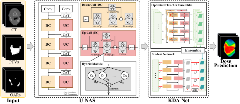
Figure 1: Overview of the proposed LENAS. $O_{i}$ in the hybrid module denotes the operation and $\alpha_{i}$ denotes its weight. $Dis$ in KDA-Net denotes the discriminator.

The framework of the proposed LENAS is shown in Fig. 1, which has two components: 1) a U-shape differentiable neural architecture search (U-NAS) pipeline for automatic architecture search, and 2) KDA-Net which hierarchically transfers the to-be-distilled knowledge of U-NAS ensembles to a single lightweight network via adversarial learning. In the following, we introduce each component in details.

III-A U-NAS

As shown in Fig. 1, the proposed U-NAS follows the autoencoder [18] structure with four down cells (DCs) and four up cells (UCs). Each individual cell is learned in a large search space with about $4\times 10^{4}$ architecture configurations. In the following, we first introduce the search space, then describe the training strategy for joint optimization of the architecture and its weights.

Search Space. The yellow and red blocks in Fig. 1 show the network topologies of DC and UC, respectively, which include several fundamental computing units called hybrid modules (HMs). Each HM is a sum of different operations, and there are four types of HM: normal ($N$), downward ($D$), upward ($U$), and connect ($C$), corresponding to different operation groups in the search space. As shown in Table I, we include the following operations in the search space: convolution (conv), squeeze-and-excitation conv (se_conv), dilated conv (dil_conv), depthwise-separable conv (dep_conv), max pooling (max_pool), average pooling (avg_pool), trilinear interpolate (interpolate), and residual connection (identity).

TABLE I: Operation set used for searching cells.

NormOps	DownOps	UpOps	ConnectOps	pre	post
identity	avg_pool	up_se_conv	identity	conv	conv
conv	max_pool	up_dep_conv	no connection
se_conv	down_se_conv	up_conv
dil_conv	down_dil_conv	up_dil_conv
dep_conv	down_dep_conv	interpolate
	down_conv

The prefix ‘down’ means the stride of the convolution operation is two, while the prefix ‘up’ indicates the transposed convolution, which doubles the image resolution. For the first three columns of Table I, we use $3\times 3\times 3$ kernels for all convolution operations int the Conv-IN-ReLU order. In addition, the $3\times 3\times 3$ convolution (pre) and $1\times 1\times 1$ convolution (post) are applied to adjust the number of channels.

Algorithm 1 Training Strategy of U-NAS

  Create the mixed operations $\overline{O}$ parametrized by $\alpha$.

  while not converged do

     1. Update weights $\omega$ by gradient descending $\nabla_{\omega}\mathcal{L}_{\mathrm{dose}}(\omega,\alpha)$ on $\mathcal{D}_{\mathrm{train}}$.

     2. Update $\alpha$ by gradient descending $\nabla_{\alpha}\mathcal{L}_{\mathrm{dose}}(\omega,\alpha)$ on $\mathcal{D}_{\mathrm{val}}$.

  end while

  Replace $\overline{O}$ with $O=O_{i}$, $i=\arg\max_{k}\exp(\alpha_{k})/\sum^{N}_{j=1}\exp(\alpha_{j})$.

  Re-train the network with the best learned cell structures on $\mathcal{D}_{\mathrm{train}}$.

Training Strategy. The training strategy of U-NAS contains two stages: the searching process and the re-training process. In the searching process, U-NAS is learned in a differentiable way [56], which optimizes a super network consisting of HMs with mixed operations. As Fig. 1 shows, for each operation $O_{i}$ in total $N$ operations $O$, the weight of each operation is determined by the parameter $\alpha_{i}\in\alpha$, whose softmax transformation $\tilde{\alpha}_{i}=\exp(\alpha_{i})/\sum^{N}_{j=1}\exp(\alpha_{j})$ represents how much $O_{i}$ contributes to the HM. Then, the architecture parameters $\alpha$ and the network weights $\omega$ are learned by the mixed operations alternately. We repeat the searching processing several times with different initializations to converge to different local optima, resulting in different searched architectures.

Once the searching process finishes, each HM would only keep the most likely operation based on the parameter $\alpha$, then we replace DCs and UCs with the best learned structure and re-train the network on $\mathcal{D}_{\mathrm{train}}$. Algorithm 1 describes the details of the training strategy of U-NAS. In both searching and re-training processes, $\mathcal{L}_{1}$ norm is used to measure the difference between the dose prediction $\hat{y}$ and the target $y$:

$$\mathcal{L}_{\mathrm{dose}}=\|y-\hat{y}\|_{1}$$ (1)

Diversity Encouraging Loss. The diversity among the models obtained by U-NAS can be potentially achieved via different initializations. However in many settings, the independently searching process could converge to similar local optima as the same searching goal is exploited. To optimize for diversity directly in the architecture searching process, we propose a diversity encouraging loss to encourage different predictions between the learned model with the best model.

Specifically, in the searching process, the goal is to achieve high accuracy of the learned model and encourage the difference of the prediction between the learned model and best model. Therefore, in the training stage of U-NAS, the final loss of $\mathcal{L}_{\mathrm{nas}}$ can be formulated by adding the dose error loss $\mathcal{L}_{\mathrm{dose}}$ in Eq. (1) with diversity encouraging loss $\mathcal{L}_{\mathrm{div}}$ as:

$$\mathcal{L}_{\mathrm{nas}} =\mathcal{L}_{\mathrm{dose}}+\mathcal{L}_{\mathrm{div}}$$ (2)

$$=\|y-\hat{y}\|_{1}+\eta\max(0,m-\frac{\left\|\hat{y}-\hat{y*}\right\|_{1}}{\left(\|\hat{y}\|_{1}+\|\hat{y*}\|_{1}\right)/2}),$$

where $\|\cdot\|_{1}$ is the voxel-wise $l_{1}$ norm; $y$, $\hat{y}$, and $\hat{y*}$ denote the ground-truth, prediction result of the training model and best model, respectively; and $m$ is the margin (empirically set to 0.2) used to reduce the correlation between $\hat{y}$ and $\hat{y*}$ while avoiding the outliers; $\eta$ is a weighting hyper-parameter to balance the two loss terms (empirically set to 1).

III-B KDA-Net

The proposed KDA-Net performs knowledge distillation from the U-NAS ensembles to a single target network with adversarial learning. As shown in Fig. 1, we use a single U-Net network as the student and the average of multiple U-NAS predictions as the teacher ensemble. For all the $K=8$ blocks (four D blocks and four C blocks) of the network, we apply the similarity loss on the intermediate output between the teacher ensembles and the student based on squared Euclidean distance as:

$$\mathcal{L}_{\mathrm{sim}}=\sum_{k=1}^{8}\left\|\frac{1}{M}\sum_{i=1}^{M}\left(I_{k}^{T_{i}}-I^{S}_{k}\right)\right\|_{2}^{2},$$ (3)

where $I^{T_{i}}_{k}$ and $I^{S}_{k}$ denote the intermediate output of the $k$-th block of the $i$-th teacher network $T$ and student network $S$, respectively, and $M$ denotes the number of teacher networks.

Then we further adopt adversarial learning in our knowledge distillation process to force the model to generate more similar features by the student and teachers. Specifically, for the $k$-th block, we learn a discriminator $D_{k}$ to distinguish the output of teachers from that of the student, which in turn encourages the student to produce more similar output with teachers. The adversarial loss is defined as:

$$\mathcal{L}_{\mathrm{adv}}=\sum_{k=1}^{8}\mathbb{E}_{I_{k}\sim P_{T}}\log D_{k}\left(I_{k}\right)+\sum_{k=1}^{8}\mathbb{E}_{I_{k}\sim P_{S}}\log\left(1-D_{k}\left(I_{k}\right)\right),$$ (4)

where $I_{k}\sim P_{T}$ and $I_{k}\sim P_{S}$ denote outputs from the $k$-th block of teacher ensembles and the student network, respectively. Based on the above definition, we incorporate the dose loss in Eq. (1), the similarity loss in Eq. (3) and the adversarial loss in Eq. (4) into our final loss function of KDA-Net:

$$\mathcal{L}_{\mathrm{KDA}}=\mathcal{L}_{\mathrm{dose}}+\lambda_{1}\mathcal{L}_{\mathrm{sim}}+\lambda_{2}\mathcal{L}_{\mathrm{adv}},$$ (5)

where $\lambda_{1}$ and $\lambda_{2}$ are weighting hyper-parameters which are empirically set to 0.05 and 0.01, respectively, in our experiments.

IV Experiments

IV-A Datasets

In this study, we evaluate the proposed method using two public datasets: the OpenKBP dataset and the AIMIS dataset.

OpenKBP dataset. The Open Knowledge-Based Planning (OpenKBP) dataset of 2020 AAPM Grand Challenge [15] is a public dataset consisting of 340 CT scans for the dose prediction task. The OpenKBP dataset includes subjects treated for head-and-neck cancer with radiation therapy. The data is partitioned into training ($n=200$), validation ($n=40$), and test ($n=100$) sets. The ROIs used in this study include the body, seven OARs (i.e., brainstem, spinal cord, right parotid, left parotid, larynx, esophagus and mandible) and three planning target volumes (PTVs) with gross disease (PTV70), intermediate-risk target volumes (PTV63), and elective target volumes (PTV56).

AIMIS dataset. The AIMIS dataset consists of 500 CT scans from the 2021 Tencent AI Medical Innovation System (AIMIS) Challenge (task 4). Each scan is from a patient treated for lung cancer with stereotactic body radiation therapy (SBRT). The dataset is officially partitioned into 300 scans for training, 100 scans for validation and 100 scans for testing. The ROIs used in this study include the body, five OARs (i.e., left lung, right lung, total lung, spinal cord, and heart) as well as inner target volume (ITV) and planning target volume (PTV).

IV-B Implementation and Evaluation Metrics

The pre-processing for the two datasets follows [57]. For normalization, the CT-values are truncated to [-1024 HU, 1500 HU]. The following data augmentations are performed during training: horizontal and vertical flips, translation, and rotation around $z$-axis. For each case of the OpenKBP dataset, the OAR masks (7 channels) and the merged target (1 channel) are concatenated with the CT scan (1 channel) as a $9\times 128\times 128\times 128$ tensor and fed into the dose prediction models. And for the AIMIS dataset, the input consists of OAR masks (5 channels), CT scan (1 channel), and target volume (2 channels) and body (1 channel).

For U-NAS, in the searching process, we first train the super network for $8\times 10^{4}$ iterations using an Adam optimizer with an initial learning rate of $3\times 10^{-4}$, and a weight decay of $1\times 10^{-4}$. After that, the architecture parameters $\alpha$ are determined from the super network on the validation set. We repeat the searching process multiple times with different random seeds to obtain various architectures. Then we re-train the searched models on the training set for $8\times 10^{4}$ iterations with a learning rate of $3\times 10^{-4}$. For KDA-Net, we train the student network for $6\times 10^{4}$ iterations using an Adam optimizer with an initial learning rate of $1\times 10^{-5}$ and weight decay of $1\times 10^{-4}$.

We use the official evaluation codes to validate the proposed method. Specifically, for the OpenKBP dataset, the evaluation metircs include: (1) dose error, which calculates the mean absolute error (MAE) between the dose prediction and its corresponding ground-truth plan with mean absolute error; and (2) DVH error, which calculates the absolute error of the DVH curves between the prediction and ground truth. According to [15], {D99, D50 D1} for PTVs and {D0.01cc, Dmean} for OARs are selected to measure the similarity of DVH curves in this task. And for the AIMIS dataset, the evaluation is performed by measuring dose error with the mean squared error (MSE). In addition, We use a paired t-test to calculate the statistical significance of the results.

TABLE II: Performance comparison of NAS models with manually designed networks on $\mathcal{D}_{val}$. And BS, SC, RP, LA, ES, LE, MD, P₇₀, P₆₃, and P₅₆ denote Brainstem, Spinal Cord, Right Parotid, Left Parotid, Larynx, Esophagus, Mandible, PTV70, PTV63, and PTV56, respectivily. $\dagger$ represents significantly different results ($p<0.05$, paired t-tests)

		Single Model					Ensemble
		Conv	Se_conv	Dil_conv	Dep_conv	NAS	Manual	NAS
Dose Error	Body	$2.634\pm 0.760$	$2.736\pm 0.861\dagger$	$2.741\pm 0.805\dagger$	$2.728\pm 0.789\dagger$	$2.581\pm 0.784$	$2.503\pm 0.762\dagger$	$2.400\pm 0.743$
	BS	$1.606\pm 1.076$	$1.646\pm 1.152$	$1.743\pm 1.305\dagger$	$1.677\pm 1.278$	$1.486\pm 0.971$	$1.541\pm 1.136$	$1.442\pm 1.035$
	SC	$2.095\pm 1.014$	$2.131\pm 1.181$	$2.184\pm 1.115$	$2.068\pm 0.986\dagger$	$2.018\pm 0.936$	$1.939\pm 0.909$	$1.891\pm 0.878$
	RP	$3.040\pm 0.870$	$3.277\pm 1.020$	$3.152\pm 0.921$	$3.472\pm 1.117$	$3.074\pm 0.909$	$2.942\pm 0.868$	$2.820\pm 0.889$
	LA	$3.154\pm 0.839$	$3.208\pm 0.979$	$3.075\pm 0.803$	$3.383\pm 1.212$	$3.029\pm 0.874$	$2.917\pm 0.740$	$2.710\pm 0.753$
	ES	$2.428\pm 1.004$	$2.773\pm 0.830$	$2.749\pm 1.036$	$2.531\pm 1.077$	$2.467\pm 1.009$	$2.410\pm 0.892$	$2.182\pm 0.705$
	LE	$3.034\pm 1.385$	$3.204\pm 1.419$	$3.451\pm 1.561$	$3.148\pm 1.481$	$2.883\pm 1.366$	$2.973\pm 1.334$	$2.593\pm 0.727$
	MD	$3.988\pm 1.341$	$3.992\pm 1.413$	$4.086\pm 1.146$	$4.051\pm 1.218$	$3.800\pm 1.189$	$3.745\pm 1.152$	$3.520\pm 1.133$
	P70	$2.062\pm 1.004\dagger$	$2.090\pm 1.167\dagger$	$2.198\pm 1.463\dagger$	$2.045\pm 0.895\dagger$	$1.620\pm 0.789$	$1.896\pm 1.108\dagger$	$1.570\pm 0.784$
	P63	$2.345\pm 1.137$	$2.534\pm 1.250\dagger$	$2.686\pm 1.566\dagger$	$2.521\pm 1.090\dagger$	$2.135\pm 0.950$	$2.318\pm 1.213\dagger$	$2.057\pm 0.926$
	P56	$2.227\pm 0.916$	$2.296\pm 0.885$	$2.326\pm 1.029\dagger$	$2.371\pm 0.758\dagger$	$2.116\pm 0.768$	$2.122\pm 0.841\dagger$	$1.926\pm 0.703$

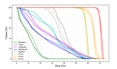
(a)

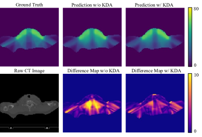
(b)

Figure 2: (a) DVHs of the dose distribution of ground-truth plan (solid curves) and predictions by a single U-Net with and without the proposed KDA method, illustrated by dashed lines and dotted curves, respectively. The PTV70, PTV63, and PTV56 are shown in red, orange, and yellow curves, respectively.(b) An example of dose distributions of the clinical plan and predicted plans of a single U-Net with and without the KDA method.

IV-C Experimental Results

IV-C1 Performance of U-NAS

We first compare the performance of our U-NAS model with four manually designed architectures on the OpenKBP validation set. For each manually designed architecture, we employ the same convolution operation choice in the normal HM, including conv, se_conv, dil_conv, and dep_conv. And we apply max_pool, interpolate and no connection operations for all the manually designed architectures. Table II shows performance comparison of different models. Our U-NAS model outperforms all the manually designed networks in the body, seven OARs and three PTVs. In summary, the single U-NAS model achieves MAE of 2.580 and 1.736 in dose score and DVH score, respectively, outperforming the best manually designed network by 0.111 and 0.128 in dose error and DVH error, respectively. And it is interesting that in most cases, the ensemble of four models outperforms the corresponding individual models (for both the manually designed and NAS learned models), and the ensemble of NAS models outperforms the ensemble of manually designed models. Please refer to Sec. V for more discussions of ensemble learning.

IV-C2 Performance of KDA-Net

We compare the performance of a single U-Net with and without the proposed KDA module, including the dose distributions and DVH, on the OpenKBP validation set. Fig. 2a shows an example of DVH curves from a patient of the validation set. The solid lines represent the DVH curves of ground truth, while the dashed lines and dotted lines represent the DVHs extracted from predicted dose of U-Net with and without KDA (i.e., train from scratch), respectively. For this example patient, the U-Net with KDA exhibits a better agreement in predicting the dose to the PTVs. The predictions of OARs are more variable between two methods. Fig. 2b shows the corresponding dose color contour for the same patient in Fig. 2a, which suggests that the single U-Net model with KDA is able to achieve better dosimetric congruence with the original plan on the PTV.

TABLE III: Comparison of performance with the state-of-the-art methods on the OpenKBP test set.

Methods		Dose Score		DVH Score
		MAE	MSE	MAE	MSE
Leaderboard	Top #1	2.429	15.488	1.478	5.913
	Top #2	2.564	16.550	1.704	6.812
	Top #3	2.615	17.774	1.582	6.961
	Top #4	2.650	18.091	1.539	6.031
	Top #5	2.679	18.023	1.573	6.525
Single Model	FCN [16]	2.681	18.144	2.452	12.310
	V-Net [17]	3.129	23.336	2.325	11.417
	U-Net [18]	2.619	17.221	2.313	11.343
	ResUNet [58]	2.601	16.932	2.209	10.591
	U-NAS (ours)	2.597	16.962	1.803	7.628
	LENAS (ours)	2.565	16.614	1.737	7.272
Cascade	U-Net [18]	2.461	15.489	1.588	6.511
	ResUNet [58]	2.448	16.023	1.499	5.855
	U-NAS (ours)	2.434	15.376	1.496	5.564
Ensemble	Off-the-shelf	2.521	16.060	1.771	6.851
	U-NAS (ours)	2.357	14.326	1.465	5.560

TABLE IV: Comparison with the state-of-the-art methods on the test set of AIMIS.

Primary Phase			Final Phase
Rank	Team	Dose Score	Rank	Team	Dose Score
#1	qqll (ours)	15611.6398	#1	qqll (ours)	15571.6051
#2	deepmedimg	17223.3940	#2	gosnail	15869.4256
#3	gosnail	18425.5708	#3	teamC	16323.9720
#4	adosepredictor	18638.4767	#4	27149	16486.1417
#5	star	19340.0643	#5	capsicummeat	18137.9836

TABLE V: Comparison of U-NAS with the off-the-shelf models on the validation set of AIMIS.

Methods	All	Body	Heart	L-Lung	R-Lung	Total	Spinal	ITV	PTV
						-Lung	-Cord
U-Net	9801	56608	45643	71894	75099	64108	68377	525499	842770
ResUNet	9782	56668	41858	77288	77399	66066	71790	593486	904382
U-NAS	9484	54839	43746	82291	71597	66922	71175	510381	858750

IV-C3 Comparison with the State-of-the-art Methods

In Table III, we compare the proposed LENAS model with several state-of-the-art methods on the OpenKBP test set. The competing methods include 3D FCN [16], V-Net [16], 3D U-Net [18], 3D ResUNet [58], and five top-ranking methods on the AAPM-2020 challenge learderboard [15]. We thoroughly compare our LENAS model with existing methods using single model, cascade and ensemble strategies. The cascade strategy is to sequentially combine two networks and produce the results in a coarse-to-fine fashion. For single model, our U-NAS achieves MAE of 2.597 and 1.803 in dose score and DVH score, respectively, outperforming the best off-the-shelf method (i.e., ResUNet). Integrating the KDA mechanism (i.e., LENAS) could further improve the performance to 2.565 and 1.737, respectively. For cascade models, our cascade U-NAS model achieves 2.434 and 1.496 MAE of dose score and DVH score, respectively, outperforming the cascade ResUNet which achieves 2.448 and 1.499. For five model ensembles, our U-NAS ensemble achieves 2.357 MAE and 14.326 MSE of dose score, and 1.465 MAE and 5.560 MSE in DVH score, outperforming the ensembles of off-the-shelf models and the top ranking solutions on the AAPM-2020 challenge leaderboard.

We further explore the generalization capability of our method on the AIMIS dataset. Specifically, we apply the best architecture learned from the OpenKBP dataset to the AIMIS challenge. The evaluation results are calculated by the organizers of the challenge, shown in Table IV. Our U-NAS method achieves the first place in the AIMIS challenge in both the primary and final phases, outperforming the runner-up by 9.36% and 1.88%, respectively. And in Table V, we further compare our U-NAS model with two best best performing off-the-shelf models, i.e., U-Net and ResUNet, with respect to different ROIs. Consistent trend can be observed that our U-NAS outperforms the off-the-shelf models and other top ranking solutions on both the validation set and the test set of AIMIS.

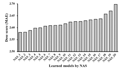
(a)

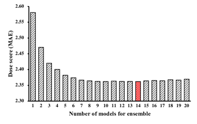
(b)

Figure 3: The dose score (MAE) of (a) 20 NAS models; (b) the ensembles.

V Discussions

In this section, we investigate the correlations between diversity and ensemble performance, and empirically provide insightful guidance for the ensemble learning with NAS in the task of dose prediction.

V-A Ensemble Many is Better than All

Most works, especially for the competitions [59, 42, 60, 61, 62], brusquely integrate all the obtained models to obtain the final result. To explore the correlation between the number of ensembles and its corresponding performance, we follow [13] to systemically conduct the searching processes multiple times and select the top 20 models for the experiment. Then, we average the results one-by-one sequentially w.r.t. the individual performance. The results are shown in Fig. 3. Fig. 3a shows the dose score of the 20 selected models which ranges from 2.5806 (NAS_1) to 2.6979 (NAS_20) in MAE. Fig. 3b shows the dose score of ensembles of top $k\in[1,20]$ models. It can be seen that the ensembles achieve best performance with top 14 models (2.3621 in MAE), instead of all the 20 models (2.3693 in MAE). Intuitively, the models in the ensembles with unacceptable performance could hurt the final ensemble results. Our next step is to explore the selection criterion for the members of the ensemble.

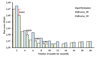
Figure 4: The dose score (MAE) of the ensembles with different numbers of models. The yellow bars indicate the models selected based on performance; the blue and green bars indicate the models selected based on diversity from top 20 models and 10 models, respectively.

V-B Performance vs. Diversity

Extensive literature [46] has shown that the ideal ensemble is one comprised of accurate networks that make errors on different parts of the input space. In other word, the performance of ensemble depends not only on the accuracy of base learners, but also the diversity of them. However, existing works typically implicitly encourage the diversity of the ensembles with different training strategies (e.g., random initializations, different hyper-parameters and loss functions), then causally select the models based on the accuracy. So does diversity matter when selecting the members in the ensemble? To answer the question, we conduct the experiments as follows.

The diversity of two models is measured by averaging the root mean absolute error (RMAE) between the predictions for each sample as follows: $d(y_{a},y_{b})=\frac{|y_{a}^{i}-y_{b}^{i}|}{y_{a}^{i}+y_{b}^{i}}$, where $y_{a}$ and $y_{b}$ are the outputs of two models. Then, we select different pairs of models based on individual models’ performance and the diversities between them. The yellow and blue bars of Fig. 4 show that for the total 20 models, the ensemble performance based on the individual models’ performance is consistently better than those based on the diversity. It reveal that the performance of individual model’s performance is an essential factor in ensembling. In addition, the results of the yellow and green bars show that in the top 10 models, the observation exactly contradicts to the former one that the ensemble performance based on the individual models’ performance are lower than those based on the diversity. It suggests that the diversity is indeed an important factor as well. Especially when the performance of the individual models are comparable, the diversity is more important than the accuracy.

(a)

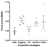
(b)

Figure 5: (a) Diversity and (b) dose score (MAE) of individual models in different ensemble strategies: NAS, bagging, random initializations and iterations, and different off-the-shelf architectures (denotes public).

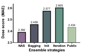
Figure 6: Overall Dose score (MAE) of the ensembles with different strategies.

V-C Comparison of Different Ensemble Strategies

A uniqueness of the proposed LENAS model is to exploit a diverse collection of network structures that drives a natural bias towards diversity of predictions produced by individual networks. To assess the impact of LENAS on the ensemble, we compare the diversity and performance of our method with four ensemble strategies on the OpenKBP validation set in Fig. 5, including bagging, random initializations, different training iterations, and different off-the-shelf architectures. For each strategy, we obtain four models randomly. Specifically, for NAS models, we select the top four models in the aforementioned 20 NAS models (i.e., NAS_1 to NAS_4). For bagging, we split the training set into four non-overlapped sub sets and using different portions of the data (three subsets) to train four models. For random initialization, we repeat the training procedures four times with different initialization seeds. For the different training epochs, we train a single network with $8\times 10^{4}$ iterations, and pick the last four checkpoints with a gap of 2000 training iterations in between. For the off-the-shelf architectures, we select the four most popular architectures in 3D medical image analysis, including FCN, VNet, U-Net, and ResUNet. The diversities of the four ensemble strategies are illustrated in Fig. 5a. The diversity of the NAS models is 0.0326 in RMAE with standard deviation of 0.0009, greater than the other three strategies (i.e., cross-validation, random initialization and iterations), comparable to off-the-shelf architectures which achieve $0.0338\pm 0.0013$ diversity. The results in Fig. 5b shows that the mean and standard deviation of the dose score of NAS models is $2.587\pm 0.0082$, outperforming other strategies by a large margin. Note that the diversity of 4-fold cross-validation is close to the NAS models; however, the individual models’ performance suffer from the limited representations of the subsets of training data. The similar trends are observed in off-the-shelf models: individual models’ performance restricts the performance of the final ensemble. The performance with respect to the dose score in MAE of the ensembles are depicted in Fig. 6. Obviously, the ensembles of NAS achieve the best performance with 2.392 in MAE, superior to the other ensemble strategies. The result reveals that producing and ensembling different network architectures is superior to those simply creating an ensemble containing duplicates of a single network architecture with different model parameters.

V-D Effectiveness of Diversity Encouraging Loss

We investigate the effectiveness of the diversity encouraging loss in Fig. 7. Specifically, we searched 10 architectures with and without diversity encouraging loss, and the learned down cells and up cells are shown in Fig. 7. We further calculate the variation of the operations in each module. Specifically, we first rank the operations in each HM based on the frequency in all the architectures (e.g., the operation with the highest frequency is identified with ID 0), then product all the std. of each HM. The quantitative results of the variation w/ and w/o diversity encouraging loss are 328.3 and 31.1, respectively, indicating that with the diversity encouraging loss, the U-NAS method can generate architectures with a greater variation, and consequently encourage the diversity of the predictions.

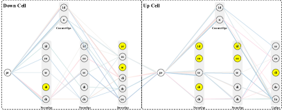
(a)

(b)

Figure 7: The down cells and up cells of 10 learned architectures (a) w/o and (b) w/ diversity encouraging loss, where id, n, co, se, di, de, av, m, in, and pr denote identity, no connection, conv, se_conv, dil_conv, dep_conv, avg_pool, max_pool, interpolate, and pre in Table I, respectively. The yellow operations are not used by the 10 architectures.

VI Conclusion and Future Work

In this paper, we proposed a learning-based ensemble approach, named LENAS, for 3D radiotherapy dose prediction. Two key components of LENAS include 1) a U-NAS framework which automatically searches the neural architectures from numerous architecture configurations to form a teacher network zoo, and 2) a KDA-Net which hierarchically transfers the distilled knowledge from the teacher networks to the student network to reduce the inference time while maintain competitive accuracy. In addition, we conducted comprehensively experiments to investigate the impact of diversity in ensemble learning, and derived several empirical guidelines for producing and ensembling multiple base learners in consideration of individual accuracy and diversity. Extensive experiments on two public datasets demonstrated the effectiveness and superior performance of our method to the state-of-the-art methods.

We would point out several limitations of our work. First, the NAS ensembles require multiple rounds of searching-retraining, which is very time-consuming in the training phase. Second, a few failure models may be generated by NAS. This situation is also common in the gradient-based NAS methods. Third, the diversity between learners in ensemble is hard to formulate appropriately, which could be task specific and vary for different outputs (e.g., classification, segmentation, and regression). Future studies will be focused on: 1) a more specific model selection criterion for the best ensemble strategies; 2) a computational-efficient training strategies for multiple ensemble learners; and 3) an optimization method from dose prediction map to the final radiotherapy treatment plan.

References

- [1] R. Atun, D. Jaffray, M. Barton, F. Bray, M. Baumann, B. Vikram, T. Hanna, F. Knaul, Y. Lievens, T. Lui, M. Milosevic, B. O’Sullivan, D. Rodin, E. Rosenblatt, J. Van Dyk, M. Yap, E. Zubizarreta, and M. Gospodarowicz, “Expanding global access to radiotherapy,” The Lancet Oncology, vol. 16, no. 10, pp. 1153–1186, Sep. 2015.
- [2] L. Lin, Q. Dou, Y.-M. Jin, G.-Q. Zhou, Y.-Q. Tang, W.-L. Chen, B.-A. Su, F. Liu, C.-J. Tao, N. Jiang et al., “Deep learning for automated contouring of primary tumor volumes by MRI for nasopharyngeal carcinoma,” Radiology, vol. 291, no. 3, pp. 677–686, 2019.
- [3] R. Van Haveren, B. J. Heijmen, and S. Breedveld, “Automatic configuration of the reference point method for fully automated multi-objective treatment planning applied to oropharyngeal cancer,” Medical Physics, vol. 47, no. 4, pp. 1499–1508, 2020.
- [4] Y. Ge and Q. J. Wu, “Knowledge-based planning for intensity-modulated radiation therapy: a review of data-driven approaches,” Medical Physics, vol. 46, no. 6, pp. 2760–2775, 2019.
- [5] D. Nguyen, T. Long, X. Jia, W. Lu, X. Gu, Z. Iqbal, and S. Jiang, “A feasibility study for predicting optimal radiation therapy dose distributions of prostate cancer patients from patient anatomy using deep learning,” Scientific Reports, vol. 9, no. 1, pp. 1–10, 2019.
- [6] J. Fan, J. Wang, Z. Chen, C. Hu, Z. Zhang, and W. Hu, “Automatic treatment planning based on three-dimensional dose distribution predicted from deep learning technique,” Medical Physics, vol. 46, no. 1, pp. 370–381, 2019.
- [7] R. N. Kandalan, D. Nguyen, N. H. Rezaeian, A. M. Barragán-Montero, S. Breedveld, K. Namuduri, S. Jiang, and M.-H. Lin, “Dose prediction with deep learning for prostate cancer radiation therapy: Model adaptation to different treatment planning practices,” Radiotherapy and Oncology, vol. 153, pp. 228–235, 2020.
- [8] D. Nguyen, X. Jia, D. Sher, M.-H. Lin, Z. Iqbal, H. Liu, and S. Jiang, “3D radiotherapy dose prediction on head and neck cancer patients with a hierarchically densely connected U-Net deep learning architecture,” Physics in Medicine & Biology, vol. 64, no. 6, p. 065020, 2019.
- [9] S. Willems, W. Crijns, E. Sterpin, K. Haustermans, and F. Maes, “Feasibility of CT-only 3D dose prediction for VMAT prostate plans using deep learning,” in Workshop on Artificial Intelligence in Radiation Therapy. Springer, 2019, pp. 10–17.
- [10] A. M. Barragán-Montero, D. Nguyen, W. Lu, M.-H. Lin, R. Norouzi-Kandalan, X. Geets, E. Sterpin, and S. Jiang, “Three-dimensional dose prediction for lung IMRT patients with deep neural networks: robust learning from heterogeneous beam configurations,” Medical Physics, vol. 46, no. 8, pp. 3679–3691, 2019.
- [11] B. Lakshminarayanan, A. Pritzel, and C. Blundell, “Simple and scalable predictive uncertainty estimation using deep ensembles,” in Advances in Neural Information Processing Systems, 2017.
- [12] G. Huang, Y. Li, G. Pleiss, Z. Liu, J. E. Hopcroft, and K. Q. Weinberger, “Snapshot ensembles: Train 1, get m for free,” in International Conference on Learning Representations, 2017.
- [13] Z.-H. Zhou, J. Wu, and W. Tang, “Ensembling neural networks: many could be better than all,” Artificial Intelligence, vol. 137, no. 1-2, pp. 239–263, 2002.
- [14] L. I. Kuncheva and C. J. Whitaker, “Measures of diversity in classifier ensembles and their relationship with the ensemble accuracy,” Machine Learning, vol. 51, no. 2, pp. 181–207, 2003.
- [15] A. Babier, B. Zhang, R. Mahmood, K. L. Moore, T. G. Purdie, A. L. M. Chan, and C. Timothy, “OpenKBP: The open-access knowledge-based planning grand challenge,” arXiv:2011.14076, 2020.
- [16] J. Long, E. Shelhamer, and T. Darrell, “Fully convolutional networks for semantic segmentation,” in Proceedings of the IEEE International Conference on Computer Vision, 2015, pp. 3431–3440.
- [17] F. Milletari, N. Navab, and S.-A. Ahmadi, “V-Net: Fully convolutional neural networks for volumetric medical image segmentation,” in The Fourth International Conference on 3D Vision. IEEE, 2016, pp. 565–571.
- [18] O. Ronneberger, P. Fischer, and T. Brox, “U-Net: Convolutional networks for biomedical image segmentation,” in International Conference on Medical Image Computing and Computer Assisted Intervention. Springer, 2015, pp. 234–241.
- [19] S. Momin, Y. Fu, Y. Lei, J. Roper, J. D. Bradley, W. J. Curran, T. Liu, and X. Yang, “Knowledge-based radiation treatment planning: A data-driven method survey,” Journal of Applied Clinical Medical Physics, vol. 22, no. 8, pp. 16–44, 2021.
- [20] X. Zhu, Y. Ge, T. Li, D. Thongphiew, F.-F. Yin, and Q. J. Wu, “A planning quality evaluation tool for prostate adaptive IMRT based on machine learning,” Medical Physics, vol. 38, no. 2, pp. 719–726, 2011.
- [21] B. Wu, F. Ricchetti, G. Sanguineti, M. Kazhdan, P. Simari, M. Chuang, R. Taylor, R. Jacques, and T. McNutt, “Patient geometry-driven information retrieval for IMRT treatment plan quality control,” Medical Physics, vol. 36, no. 12, pp. 5497–5505, 2009.
- [22] T. Kajikawa, N. Kadoya, K. Ito, Y. Takayama, T. Chiba, S. Tomori, H. Nemoto, S. Dobashi, K. Takeda, and K. Jingu, “A convolutional neural network approach for IMRT dose distribution prediction in prostate cancer patients,” Journal of Radiation Research, vol. 60, no. 5, pp. 685–693, 2019.
- [23] G. Bohara, A. Sadeghnejad Barkousaraie, S. Jiang, and D. Nguyen, “Using deep learning to predict beam-tunable pareto optimal dose distribution for intensity-modulated radiation therapy,” Medical Physics, vol. 47, no. 9, pp. 3898–3912, 2020.
- [24] J. Ma, T. Bai, D. Nguyen, M. Folkerts, X. Jia, W. Lu, L. Zhou, and S. Jiang, “Individualized 3D dose distribution prediction using deep learning,” in Workshop on Artificial Intelligence in Radiation Therapy. Springer, 2019, pp. 110–118.
- [25] T. I. Götz, C. Schmidkonz, S. Chen, S. Al-Baddai, T. Kuwert, and E. W. Lang, “A deep learning approach to radiation dose estimation,” Physics in Medicine & Biology, vol. 65, no. 3, p. 035007, 2020.
- [26] Z. Liu, J. Fan, M. Li, H. Yan, Z. Hu, P. Huang, Y. Tian, J. Miao, and J. Dai, “A deep learning method for prediction of three-dimensional dose distribution of helical tomotherapy,” Medical Physics, vol. 46, no. 5, pp. 1972–1983, 2019.
- [27] Y. Murakami, T. Magome, K. Matsumoto, T. Sato, Y. Yoshioka, and M. Oguchi, “Fully automated dose prediction using generative adversarial networks in prostate cancer patients,” PloS One, vol. 15, no. 5, p. e0232697, 2020.
- [28] D. Nguyen, R. McBeth, A. Sadeghnejad Barkousaraie, G. Bohara, C. Shen, X. Jia, and S. Jiang, “Incorporating human and learned domain knowledge into training deep neural networks: A differentiable dose-volume histogram and adversarial inspired framework for generating pareto optimal dose distributions in radiation therapy,” Medical Physics, vol. 47, no. 3, pp. 837–849, 2020.
- [29] S. Tan, P. Tang, X. Peng, J. Xiao, C. Zu, X. Wu, J. Zhou, and Y. Wang, “Incorporating isodose lines and gradient information via multi-task learning for dose prediction in radiotherapy,” in International Conference on Medical Image Computing and Computer Assisted Intervention. Springer, 2021, pp. 753–763.
- [30] O. Russakovsky, J. Deng, H. Su, J. Krause, S. Satheesh, S. Ma, Z. Huang, A. Karpathy, A. Khosla, M. Bernstein et al., “ImageNet large scale visual recognition challenge,” International Journal of Computer Vision, vol. 115, no. 3, pp. 211–252, 2015.
- [31] P. Domingos, “Bayesian averaging of classifiers and the overfitting problem,” in International Conference on Machine Learning, vol. 747. Citeseer, 2000, pp. 223–230.
- [32] K. Monteith, J. L. Carroll, K. Seppi, and T. Martinez, “Turning Bayesian model averaging into Bayesian model combination,” in The 2011 International Joint Conference on Neural Networks. IEEE, 2011, pp. 2657–2663.
- [33] P. M. Domingos, “Why does bagging work? A Bayesian account and its implications.” in Proceedings of ACM SIGKDD International Conference on Knowledge Discovery and Data Mining. Citeseer, 1997, pp. 155–158.
- [34] T. G. Dietterich, “Ensemble methods in machine learning,” in International Workshop on Multiple Classifier Systems. Springer, 2000, pp. 1–15.
- [35] Z.-H. Zhou, “Ensemble learning,” in Machine Learning. Springer, 2021, pp. 181–210.
- [36] G. Brown, J. L. Wyatt, P. Tino, and Y. Bengio, “Managing diversity in regression ensembles.” Journal of Machine Learning Research, vol. 6, no. 9, pp. 1621–1650, 2005.
- [37] M.-L. Zhang and Z.-H. Zhou, “Exploiting unlabeled data to enhance ensemble diversity,” Data Mining and Knowledge Discovery, vol. 26, no. 1, pp. 98–129, 2013.
- [38] N. Altman and M. Krzywinski, “Ensemble methods: bagging and random forests,” Nature Methods, vol. 14, no. 10, pp. 933–935, 2017.
- [39] S. Kornblith, M. Norouzi, H. Lee, and G. Hinton, “Similarity of neural network representations revisited,” in International Conference on Machine Learning. PMLR, 2019, pp. 3519–3529.
- [40] A. S. Morcos, M. Raghu, and S. Bengio, “Insights on representational similarity in neural networks with canonical correlation,” in Advances in Neural Information Processing Systems, 2018, pp. 5732–5741.
- [41] N. Srivastava, G. Hinton, A. Krizhevsky, I. Sutskever, and R. Salakhutdinov, “Dropout: a simple way to prevent neural networks from overfitting,” The Journal of Machine Learning Research, vol. 15, no. 1, pp. 1929–1958, 2014.
- [42] Y. Lin, H.-Y. Zhou, K. Ma, X. Yang, and Y. Zheng, “Seg4Reg networks for automated spinal curvature estimation,” in International Workshop and Challenge on Computational Methods and Clinical Applications for Spine Imaging. Springer, 2019, pp. 69–74.
- [43] K. He, X. Zhang, S. Ren, and J. Sun, “Deep residual learning for image recognition,” in Proceedings of the IEEE/CVF Conference on Computer Vision and Pattern Recognition, 2016, pp. 770–778.
- [44] G. Huang, Z. Liu, L. Van Der Maaten, and K. Q. Weinberger, “Densely connected convolutional networks,” in Proceedings of the IEEE/CVF Conference on Computer Vision and Pattern Recognition, 2017, pp. 4700–4708.
- [45] M. Tan and Q. Le, “EfficientNet: Rethinking model scaling for convolutional neural networks,” in International Conference on Machine Learning. PMLR, 2019, pp. 6105–6114.
- [46] D. W. Opitz and J. W. Shavlik, “Actively searching for an effective neural network ensemble,” Connection Science, vol. 8, no. 3-4, pp. 337–354, 1996.
- [47] M. PERRONE, “When networks disagree: Ensemble methods for hybrid neural networks,” Neural Networks for Speech and Image Processing, 1993.
- [48] V. Dondeti, J. D. Bodapati, S. N. Shareef, and N. Veeranjaneyulu, “Deep convolution features in non-linear embedding space for fundus image classification.” Revue d’Intelligence Artificielle, vol. 34, no. 3, pp. 307–313, 2020.
- [49] C. Jiang, S. Wang, X. Liang, H. Xu, and N. Xiao, “ElixirNet: Relation-aware network architecture adaptation for medical lesion detection,” in Proceedings of the AAAI Conference on Artificial Intelligence, vol. 34, no. 07, 2020, pp. 11 093–11 100.
- [50] X. Wang, T. Xiang, C. Zhang, Y. Song, D. Liu, H. Huang, and W. Cai, “BiX-NAS: Searching efficient bi-directional architecture for medical image segmentation,” in International Conference on Medical Image Computing and Computer Assisted Intervention. Springer, 2021, pp. 229–238.
- [51] J. Yan, S. Chen, Y. Zhang, and X. Li, “Neural architecture search for compressed sensing magnetic resonance image reconstruction,” Computerized Medical Imaging and Graphics, vol. 85, p. 101784, 2020.
- [52] Y. Weng, T. Zhou, Y. Li, and X. Qiu, “NAS-UNet: Neural architecture search for medical image segmentation,” IEEE Access, vol. 7, pp. 44 247–44 257, 2019.
- [53] Z. Zhu, C. Liu, D. Yang, A. Yuille, and D. Xu, “V-NAS: Neural architecture search for volumetric medical image segmentation,” in International Conference on 3D Vision. IEEE, 2019, pp. 240–248.
- [54] E. Real, A. Aggarwal, Y. Huang, and Q. V. Le, “Regularized evolution for image classifier architecture search,” in Proceedings of the AAAI Conference on Artificial Intelligence, vol. 33, no. 01, 2019, pp. 4780–4789.
- [55] B. Zoph, V. Vasudevan, J. Shlens, and Q. V. Le, “Learning transferable architectures for scalable image recognition,” in Proceedings of the IEEE/CVF Conference on Computer Vision and Pattern Recognition, 2018, pp. 8697–8710.
- [56] H. Liu, K. Simonyan, and Y. Yang, “DARTS: Differentiable architecture search,” in International Conference on Learning Representations, 2019.
- [57] S. Liu, J. Zhang, T. Li, H. Yan, and J. Liu, “A cascade 3d U-Net for dose prediction in radiotherapy,” Medical Physics, vol. 48, no. 9, pp. 5574–5582, 2021.
- [58] L. Yu, X. Yang, H. Chen, J. Qin, and P. A. Heng, “Volumetric ConvNets with mixed residual connections for automated prostate segmentation from MR images,” in Proceedings of the AAAI Conference on Artificial Intelligence, vol. 31, no. 1, 2017.
- [59] P. Tang, Q. Liang, X. Yan, S. Xiang, and D. Zhang, “GP-CNN-DTEL: Global-part CNN model with data-transformed ensemble learning for skin lesion classification,” IEEE Journal of Biomedical and Health Informatics, vol. 24, no. 10, pp. 2870–2882, 2020.
- [60] L. Deng and J. Platt, “Ensemble deep learning for speech recognition,” in Proceedings of Interspeech, 2014.
- [61] M. Fernández-Delgado, E. Cernadas, S. Barro, and D. Amorim, “Do we need hundreds of classifiers to solve real world classification problems?” The Journal of Machine Learning Research, vol. 15, no. 1, pp. 3133–3181, 2014.
- [62] D. Ghimire and J. Lee, “Extreme learning machine ensemble using bagging for facial expression recognition,” Journal of Information Processing Systems, vol. 10, no. 3, pp. 443–458, 2014.