• We consider the dressed energy $\varepsilon$ of the XXZ chain in the massless antiferromagnetic parameter regime at $0<\Delta<1$ and at finite magnetic field. This function is defined as a solution of a Fredholm integral equation of the second kind. Conceived as a real function over the real numbers it describes the energy of particle-hole excitations over the ground state at fixed magnetic field. The extension of the dressed energy to the complex plane determines the solutions to the Bethe Ansatz equations for the eigenvalue problem of the quantum transfer matrix of the model in the low-temperature limit. At low temperatures the Bethe roots that parametrize the dominant eigenvalue of the quantum transfer matrix come close to the curve ${\rm Re}\,\varepsilon(\lambda)=0$. We describe this curve and give lower bounds to the function ${\rm Re}\,\varepsilon$ in regions of the complex plane, where it is positive.

1 Introduction

The XXZ chain [13, 18, 19, 20, 21] is an anisotropic deformation of the Heisenberg chain [2]. It is the prototypical example of a Yang-Baxter integrable model which is solvable by means of the algebraic Bethe Ansatz [14]. The Hamiltonian of the model acts on the tensor product space ${\cal H}_{L}=\bigotimes_{j=1}^{L}V_{j}$, $V_{j}={\mathbb{C}}^{2}$, in which every factor is identified with a lattice site in a 1d crystal. Expressed in terms of the familiar Pauli matrices $\sigma^{\alpha}\in\operatorname{End}{\mathbb{C}}^{2}$, $\alpha=x,y,z$, the Hamiltonian takes the form

$$H_{L}=J\sum_{j=1}^{L}\Bigl{\{}\sigma_{j-1}^{x}\sigma_{j}^{x}+\sigma_{j-1}^{y}\sigma_{j}^{y}+\Delta\bigl{(}\sigma_{j-1}^{z}\sigma_{j}^{z}-1\bigr{)}\Bigr{\}}-\frac{h}{2}\sum_{j=1}^{L}\sigma_{j}^{z}\,.$$ (1)

The three real parameters involved in this definition are the anisotropy $\Delta$, the exchange interaction $J>0$, and the strength $h>0$ of an external magnetic field.

The functions that characterize the properties of Yang-Baxter integrable quantum systems in the thermodynamic limit, $L\rightarrow\infty$, at zero temperature are defined as solutions of Fredholm integral equations of the second kind with kernels of difference form. The kernel functions $K$ are given by the derivatives of the bare two-particle scattering phases $\theta$ as functions of a rapidity variable $\lambda$. If $S(\lambda)$ is the two-particle scattering factor for a given $\lambda$, then $S(\lambda)=\operatorname{e}^{2\pi{\rm i}\theta(\lambda)}$ and $K(\lambda)=\theta^{\prime}(\lambda)$.

For the XXZ chain with anisotropy parameter $\Delta=\cos(\gamma)$ we have

$$S(\lambda)=\frac{\operatorname{sh}(\lambda-{\rm i}\gamma)}{\operatorname{sh}(\lambda+{\rm i}\gamma)}\,.$$ (2)

Hence, the kernel function is

$$K(\lambda|\gamma)=\frac{1}{2\pi{\rm i}}\bigl{(}\operatorname{cth}(\lambda-{\rm i}\gamma)-\operatorname{cth}(\lambda+{\rm i}\gamma)\bigr{)}\,.$$ (3)

In the following we restrict ourselves to the so-called repulsive critical regime $0<\Delta<1$ corresponding to $\gamma\in(0,\pi/2)$.

We consider the integral equation

$$f(\lambda|Q)=f_{0}(\lambda)-\int_{-Q}^{Q}{\rm d}\mu\;K(\lambda-\mu|\gamma)f(\mu|Q)\,,$$ (4)

where $f_{0}\in C^{0}\bigl{(}[-Q,Q]\bigr{)}$ will be called the driving term. It is not difficult to establish the existence and uniqueness of solutions of (4) on $C^{0}\bigl{(}[-Q,Q]\bigr{)}$. It follows from the convergence of the Neumann series of the corresponding integral operator. The proof and some further implications will be recalled below.

Once $f(\cdot|Q)\in C^{0}\bigl{(}[-Q,Q]\bigr{)}$ is fixed, the integral on the right hand side of (4) defines a holomorphic ${\rm i}\pi$-periodic function on the domain

$$\Upsilon_{\gamma}(Q)=\bigl{\{}z\in{\mathbb{C}}\big{|}z\notin[-Q,Q]\pm{\rm i}\gamma\mod{\rm i}\pi\bigr{\}}\,.$$ (5)

If $f_{0}$ is meromorphic and ${\rm i}\pi$-periodic on $\Upsilon_{\gamma}(Q)$, then the same is true for $f(\cdot|Q)$ due to (4). Functions defined this way play an important role in the study of correlation functions of the XXZ chain in the zero-temperature limit (see e.g. [11, 10, 3]).

The purpose of this work is to gain a better understanding of one such special function, the dressed energy, on $\Upsilon_{\gamma}(Q)$. Consider (4) with driving term

$$\varepsilon_{0}(\lambda)=h-4\pi J\sin(\gamma)K(\lambda|\gamma/2)\,.$$ (6)

This function is even on ${\mathbb{R}}$ and monotonically increasing on ${\mathbb{R}}_{+}$.

$$\min_{\lambda\in{\mathbb{R}}}\varepsilon_{0}(\lambda)=\varepsilon_{0}(0)=h-4\pi J\sin(\gamma)K(0|\gamma/2)=h-4J(1+\Delta)\,.$$ (7)

The condition $\varepsilon_{0}(0)=0$ determines the ‘upper critical field’

$$h_{c}=4J(1+\Delta)\,.$$ (8)

Since $\lim_{\lambda\rightarrow\infty}\varepsilon_{0}(\lambda)=h$, the function $\varepsilon_{0}$ has a unique positive zero $Q_{0}$ if and only if

$$0<h<h_{c}\,.$$ (9)

The latter condition defines the ‘critical parameter regime’. The solution $\varepsilon(\lambda|Q)$ of (4) with driving term $\varepsilon_{0}(\lambda)$ has the following properties.

Theorem 1.

Existence and uniqueness of Fermi points [4]. Let $\gamma\in(0,\pi/2)$ and

$$\varepsilon_{u}(\lambda)=h-\frac{2\pi J\sin(\gamma)}{\gamma\operatorname{ch}(\pi\lambda/\gamma)}\,.$$ (10)

1. The function $\varepsilon(\lambda|Q)$ is a smooth function of $(\lambda,Q)$ on ${\mathbb{R}}\times(0,\infty)$ that is even in $\lambda$.

2. For $\lambda\in{\mathbb{R}}$ it has the lower and upper bounds

   $$\varepsilon_{0}(\lambda)<\varepsilon(\lambda|Q) 0<Q\leq Q_{0}$$ for , (11a)

   $$\varepsilon(\lambda|Q)<\varepsilon_{u}(\lambda) Q\geq 0$$ for all . (11b)

3. For any $h\in(0,h_{c})$ exists a unique solution $Q_{F}>0$ of the equation $\varepsilon(Q|Q)=0$. $Q_{F}$ is called the Fermi rapidity.

4. The Fermi rapidity is bounded by

   $$Q_{F}<Q_{0}$$ (12a)

   and, if there is a $$Q_{u} \varepsilon_{u}(Q_{u})=0 \Leftrightarrow h<2\pi J\sin(\gamma)/\gamma$$ with (), by

   $$Q_{u}<Q_{F}\,.$$ (12b)

5. The function $h:(0,h_{c})\rightarrow{\mathbb{R}}_{+}$, $h\mapsto Q_{F}$ is smooth and monotonically decreasing with $\lim_{h\rightarrow 0}Q_{F}=\infty$ and $\lim_{h\rightarrow h_{c}}Q_{F}=0$.

Remark.

The proof of this theorem given in [4] is only valid for $h<2\pi J\sin(\gamma)/\gamma$, which is the condition for $Q_{u}$ to exist. But it can be readily extended to the whole interval $(0,h_{c})$ (see below).

We define the dressed energy by

$$\varepsilon(\lambda)=\varepsilon(\lambda|Q_{F})\,.$$ (13)

A dressed energy function was introduced in the context of the Bose gas with delta function interaction in [22]. The dressed energy (13) of the XXZ chain in the critical regime first appeared [17] in the low temperature limit of the TBA equations that fix the thermodynamic properties of the XXZ chain.

The dressed energy is a meromorphic ${\rm i}\pi$-periodic function on $\Upsilon_{\gamma}(Q_{F})$ by construction. Alternatively, we may interpret it as a function on the cylinder with cuts

$$S_{\gamma}(Q_{F})=\Upsilon_{\gamma}(Q_{F})\cap\bigl{\{}z\in{\mathbb{C}}\big{|}-\pi/2\leq{\rm Im\,}z<\pi/2\bigr{\}}\,.$$ (14)

By the implicit function theorem the equation

$${\rm Re\,}\varepsilon(\lambda)=0$$ (15)

determines a smooth curve on $S_{\gamma}(Q_{F})$. This curve and the functions ${\rm Re\,}\varepsilon$ and ${\rm Im\,}\varepsilon$ are further characterized by the following theorem.

Theorem 2.

Dressed energy in the complex plane. Let $\gamma\in(0,\pi/2)$ and $\varepsilon$ be as in (13).

1. For all $\lambda\in S_{\gamma}(Q_{F})$ with ${\rm Re\,}\lambda=x$ and ${\rm Im\,}\lambda=y$ the function $\lambda\mapsto{\rm Re\,}\varepsilon(\lambda)$ is even in $x$ and in $y$.

2. Within the strip $0\leq y<\gamma/2$ the function $x\mapsto{\rm Re\,}\varepsilon(x+{\rm i}y)$ is monotonically increasing on ${\mathbb{R}}_{+}$ and, for every $y$, has a single simple zero $x(y)$.

3. This determines a smooth function $x(y)$ on $(0,\gamma/2)$ which behaves at the boundaries as $x(0)=Q_{F}$ and

   $$x(y)\sim\sqrt{\frac{2J\sin(\gamma)}{c}\biggl{(}\frac{\gamma}{2}-y\biggr{)}}$$ (16)

   with

   $$c=\frac{1}{1-\frac{\gamma}{\pi}}\biggl{\{}\frac{h}{2}+\int_{Q_{F}}^{\infty}{\rm d}\mu\>K\biggl{(}\frac{\mu}{1-\frac{\gamma}{\pi}}\Big{|}\frac{\gamma/2}{1-\frac{\gamma}{\pi}}\biggr{)}\varepsilon(\mu)\biggr{\}}>0$$ (17)

   for $y\rightarrow(\gamma/2)_{-}$.

4. Within the strip $|{\rm Im\,}\lambda|<\gamma/2$ the dressed energy is subject to the bounds

   $${\rm Re\,}\varepsilon_{0}(\lambda)<{\rm Re\,}\varepsilon(\lambda)<{\rm Re\,}\varepsilon_{u}(\lambda)\,.$$ (18)

5. ${\rm Re\,}\varepsilon(\lambda)>0$ for all $\lambda\in S_{\gamma}(Q_{F})$ with $|{\rm Im\,}\lambda|>\gamma/2$, and we have the lower bounds

   $${\rm Re\,}\varepsilon(\lambda)>h \text{if}\quad\frac{\pi}{2}-\frac{1}{2}\biggl{(}\frac{\pi}{2}-\gamma\biggr{)}<y<\frac{\pi}{2}\,,$$ (19a)

   $${\rm Re\,}\varepsilon(\lambda)>\frac{h}{2} \text{if}\quad\gamma<y<\frac{\pi}{2}-\frac{1}{2}\biggl{(}\frac{\pi}{2}-\gamma\biggr{)}\,,$$ (19b)

   $${\rm Re\,}\varepsilon(\lambda)>\min\biggl{\{}\frac{h}{2},\frac{h\gamma}{\pi-\gamma}\biggr{\}} \text{if}\quad\frac{\gamma}{2}<y<\gamma\,.$$ (19c)

6. For all $\lambda\in S_{\gamma}(Q_{F})$ with ${\rm Re\,}\lambda=x$ and ${\rm Im\,}\lambda=y$ the function $\lambda\mapsto{\rm Im\,}\varepsilon(\lambda)$ is odd in $x$ and in $y$.

7. ${\rm Im\,}\varepsilon$ is monotonically increasing along the curve $x(y)$,

   $$\frac{{\rm d}\,{\rm Im\,}\varepsilon(x(y)+{\rm i}y)}{{\rm d}y}>0\,,$$ (20)

   ${\rm Im\,}\varepsilon(x(0))=0$ and

   $${\rm Im\,}\varepsilon(x(y)+{\rm i}y)\sim\sqrt{\frac{2J\sin(\gamma)c}{\gamma/2-y}}$$ (21)

   for $y\rightarrow(\gamma/2)_{-}$.

This theorem is our main result. It will be proven below. Examples of the curve (15) for various sets of parameters are shown in Fig. 1. Our

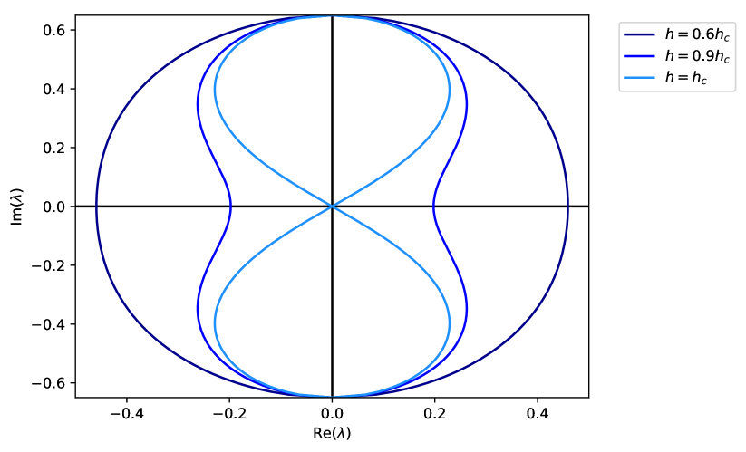
Figure 1: The curves (15) for $J=1$, $\gamma=1.3$ and various values of the magnetic field in units of $h_{c}=5.07$. Loosely speaking, Theorem 2 says that the figure describes the generic situation: ${\rm Re\,}\varepsilon(\lambda)=0$ is a simple closed curve, situated entirely inside the strip $|{\rm Im\,}\lambda|<\frac{\gamma}{2}$, symmetric with respect to the real and imaginary axis, such that its positive part, ${\rm Re\,}\lambda>0$, is the graph $\{x(y)+{\rm i}y|y\in(-\gamma/2,\gamma/2)\}$ of a smooth function $x(y)$. At $h=h_{c}$ this graph develops a cusp which signals the transition to the fully polarized massive regime.

interest in the curve (15) and in the estimates (19) comes from our work on thermal form factor series for the correlation functions of the XXZ chain (see e.g. [3, 7, 9, 1]). The derivation of the series requires knowledge of the full spectrum of the quantum transfer matrix [16, 15, 12] of the model. So far we have found a characterization of the full spectrum only in the massive antiferromagnetic regime ($\Delta>1$ and $0<h<h_{\ell}$, where $h_{\ell}$ is a lower critical field) in the low-temperature limit [6]. This case is characterized by the absence of so-called string excitations. Theorem 2 will be needed in order to establish a similar behaviour in the massless regime. This is what we would like to achieve in a subsequent paper. It will be dealing with the low-temperature analysis of the auxiliary functions and the spectrum of the quantum transfer matrix of the XXZ chain for $-1<\Delta<1$. The ‘critical part of the spectrum’, pertaining to excitations about the two Fermi points $\pm Q_{F}$, was analyzed in [3, 5]. In our forthcoming work we want to exclude the existence of strings in the low-temperature limit. This will show that not only the Bethe roots of the dominant state, but the Bethe roots belonging to any Bethe eigenstate of the quantum transfer matrix come close to the curve ${\rm Re\,}\varepsilon(\lambda)=0$, when the temperature goes to zero. The latter will then be a crucial input for the further investigation of the thermal form factor series of the two-point functions of the XXZ chain in the critical regime.

Our two theorems above are stated for a restricted parameter regime, $\gamma\in(0,\pi/2)$. This has several reasons. First of all we wanted to avoid further case distinctions in order to keep this work reasonably short and reader-friendly. In fact a version of Theorem 1 valid for $\gamma\in(\pi/2,\pi)$ can be found in [4]. As for the extension of Theorem 2, the techniques developed in [4] and below can be used. There are, however, certain technical difficulties which come from the fact that for $\gamma>2\pi/3$ the pole of the driving term $\varepsilon_{0}$ is beyond the cuts caused by the poles of the kernel function inside the fundamental cylinder, which are, in this case, located at $[-Q_{F},Q_{F}]\pm{\rm i}(\pi-\gamma)$. These problems can be dealt with by a deformation of the integration contour in the integral equation (4), but this is more naturally done in conjunction with the low-$T$ analysis of the non-linear integral equations for the auxiliary functions. We would also like to point out that for some of the proofs of the properties of $\varepsilon$ for $\gamma\in(0,\pi/2)$ we will need to know the properties of the kernel function for $\gamma\in(0,\pi)$, which is why Lemma 1 below is formulated for the extended parameter region.

2 Preliminaries

2.1 Properties of the kernel function

At several instances we will use Fourier transformation techniques. Our convention for the Fourier transform of a function $f:{\mathbb{C}}\rightarrow{\mathbb{C}}$ is

$${\cal F}[f](k)=\int_{-\infty}^{\infty}{\rm d}\lambda\>\operatorname{e}^{{\rm i}k\lambda}f(\lambda)\,.$$ (22)

Lemma 1.

Properties of the kernel function.

1. $K(\cdot|\gamma)$ defines a smooth even function on ${\mathbb{R}}$ which is monotonously decreasing on ${\mathbb{R}}_{+}$ if $0<\gamma<\pi/2$ and monotonously increasing on ${\mathbb{R}}_{+}$ if $\pi/2<\gamma<\pi$.

2. $K(\lambda|\gamma)>0$ for all $\lambda\in{\mathbb{R}}$ if $0<\gamma<\pi/2$, and $K(\lambda|\gamma)<0$ for all $\lambda\in{\mathbb{R}}$ if $\pi/2<\gamma<\pi$.

3. $K(\cdot|\gamma)$ is meromorphic on $S_{\gamma}(Q)$ with two simple poles which are located at $\pm{\rm i}\gamma$ if $0<\gamma<\pi/2$ or at $\pm{\rm i}(\pi-\gamma)$ if $\pi/2<\gamma<\pi$.

4. For $x,y\in{\mathbb{R}}$

   $${\rm Re\,}K(x+{\rm i}y|\gamma)=\frac{1}{2}\bigl{(}K(x|\gamma-y)+K(x|\gamma+y)\bigr{)}\,,$$ (23)

   implying that ${\rm Re\,}K(x+{\rm i}y|\gamma)$ is an even function of $x$ for fixed $y$ and an even function of $y$ for fixed $x$.

5. $${\cal F}[K(\cdot|\gamma)](k)=\frac{\operatorname{sh}((\pi/2-\gamma)k)}{\operatorname{sh}(\pi k/2)}\,.$$ (24)

Proof.

The kernel function $K(\lambda|\gamma)$ can be rewritten as

$$K(\lambda|\gamma)=\frac{\sin(2\gamma)}{2\pi\bigl{(}\operatorname{sh}^{2}(\lambda)+\sin^{2}(\gamma)\bigr{)}}$$ (25)

from which we can read of (i) and (ii). (iii) and (iv) are direct consequences of the definition (3). The calculation of the Fourier transform (v) is a standard exercise using the ${\rm i}\pi$-periodicity of $K(\cdot|\gamma)$ and the residue theorem. ∎

2.2 The solvable case $Q=\infty$

For $Q=\infty$ the integral equation (4) can be solved by means of Fourier transformation and the convolution theorem. This gives us explicit solutions for various driving terms $f_{0}$. As we shall see, some of these play an important role as bounds for the general case of finite $Q$. The most important such function is the resolvent kernel $R(\cdot|\gamma)$. It is the solution of (4) for $Q=\infty$ and with driving term $f_{0}(\lambda)=K(\lambda-\mu|\gamma)$.

Lemma 2.

Properties of the resolvent kernel for $Q=\infty$ [21].

1. The resolvent kernel $R(\cdot|\gamma)$ has the Fourier integral representation

   $$R(\lambda|\gamma)=\int_{-\infty}^{\infty}\frac{{\rm d}k}{4\pi}\frac{\operatorname{e}^{-{\rm i}k\lambda}\operatorname{sh}\bigl{(}(\pi/2-\gamma)k\bigr{)}}{\operatorname{ch}(\gamma k/2)\operatorname{sh}\bigl{(}(\pi-\gamma)k/2\bigr{)}}\,,$$ (26)

   valid for $|{\rm Im\,}\lambda|<\gamma$.

2. For $0<\gamma<\pi/2$, $R(\cdot|\gamma)$ has the convolution type representation

   $$R(\lambda|\gamma)=\frac{\pi}{2\gamma(\pi-\gamma)}\int_{-\infty}^{\infty}{\rm d}\mu\>\frac{K\Bigl{(}\frac{\mu}{1-\frac{\gamma}{\pi}}\Big{|}\frac{\gamma/2}{1-\frac{\gamma}{\pi}}\Bigr{)}}{\operatorname{ch}\bigl{(}(\lambda-\mu)\frac{\pi}{\gamma}\bigr{)}}\,,$$ (27)

   valid for $|{\rm Im\,}\lambda|<\gamma/2$.

3. For $0<\gamma<\pi/2$, $R(\cdot|\gamma)$ is even and positive on ${\mathbb{R}}$ and monotonically decreasing on ${\mathbb{R}}_{+}$, where it satisfies $\lim_{\lambda\rightarrow\infty}R(\lambda|\gamma)=0$.

Proof.

(i) Fourier transforming the integral equation

$$R(\lambda|\gamma)=K(\lambda|\gamma)-\int_{-\infty}^{\infty}{\rm d}\mu\>K(\lambda-\mu|\gamma)R(\mu|\gamma)$$ (28)

and solving for ${\cal F}[R(\cdot|\gamma)]$ we obtain

$${\cal F}[R(\cdot|\gamma)](k)=\frac{\operatorname{sh}\bigl{(}(\pi/2-\gamma)k\bigr{)}}{2\operatorname{ch}(\gamma k/2)\operatorname{sh}\bigl{(}(\pi-\gamma)k/2\bigr{)}}\,.$$ (29)

For $k\rightarrow\pm\infty$ we see that ${\cal F}[R(\cdot|\gamma)](k)\sim\operatorname{e}^{-\gamma|k|}$, implying that the back transformation (26) converges for all $\lambda$ with $|{\rm Im\,}\lambda|<\gamma$.

(ii) The convolution type representation is obtained from (26) by rescaling $k\rightarrow k/(1-\gamma/\pi)$ and setting

$$\gamma^{\prime}=\frac{\gamma/2}{1-\gamma/\pi}\,.$$ (30)

Then

$$R(\lambda|\gamma)=\frac{1}{1-\gamma/\pi}\int_{-\infty}^{\infty}\frac{{\rm d}k}{4\pi}\frac{\operatorname{e}^{-{\rm i}\frac{k\lambda}{1-\gamma/\pi}}}{\operatorname{ch}(\gamma^{\prime}k)}{\cal F}[K(\cdot|\gamma^{\prime})](k)\,,$$ (31)

which implies (27) by employing the convolution theorem on the right hand side. Note that $\gamma\mapsto\gamma^{\prime}$ is a monotonically increasing function that maps $(0,\pi/2)\rightarrow(0,\pi/2)$. Because of the poles of $K(\cdot/(1-\gamma/\pi)|\gamma^{\prime})$ and $1/\operatorname{ch}(\cdot\>\pi/\gamma)$ at $\pm{\rm i}\gamma/2$ the validity of the representation (27) is restricted to $|{\rm Im\,}\lambda|<\gamma/2$.

(iii) From the representation (27) it is clear that $R(\lambda|\gamma)>0$ and that $R(\lambda|\gamma)$ is even in $\lambda$. Both, $K(\lambda/(1-\gamma/\pi)|\gamma^{\prime})$ and $1/\operatorname{ch}(\lambda\pi/\gamma)$, are even, positive, integrable over ${\mathbb{R}}$, and go to zero monotonically for $\lambda\rightarrow\pm\infty$. For any two kernels $K_{1}$, $K_{2}$ with these properties and all $\lambda>0$ we have the estimate

$$\int_{-\infty}^{\infty}{\rm d}\mu\>K_{1}(\lambda-\mu)K_{2}(\mu)\\ <K_{1}(\lambda/2)\int_{-\infty}^{\lambda/2}{\rm d}\mu\>K_{2}(\mu)+K_{2}(\lambda/2)\int_{\lambda/2}^{\infty}{\rm d}\mu\>K_{1}(\lambda-\mu)\,.$$ (32)

Hence, (27) implies that $\lim_{\lambda\rightarrow\pm\infty}R(\lambda|\gamma)=0$.

Furthermore,

$$R^{\prime}(\lambda|\gamma)=\frac{1}{2\gamma(1-\gamma/\pi)^{2}}\int_{0}^{\infty}{\rm d}\mu\>K^{\prime}\Bigl{(}\frac{\mu}{1-\gamma/\pi}\Big{|}\gamma^{\prime}\Bigr{)}\\ \times\biggl{\{}\frac{1}{\operatorname{ch}\bigl{(}(\lambda-\mu)\frac{\pi}{\gamma}\bigr{)}}-\frac{1}{\operatorname{ch}\bigl{(}(\lambda+\mu)\frac{\pi}{\gamma}\bigr{)}}\biggr{\}}\,.$$ (33)

Now $1/\operatorname{ch}$ is even and monotonically decreasing on ${\mathbb{R}}_{+}$, and $|\lambda-\mu|<\lambda+\mu$ for all $\lambda,\mu\in{\mathbb{R}}_{+}$, implying that the term in the curly brackets under the integral is positive. Since $K^{\prime}(\mu/(1-\gamma/\pi)|\gamma^{\prime})<0$ for $\mu>0$, it follows that $R^{\prime}(\lambda|\gamma)<0$ for all $\lambda>0$. ∎

Two more ‘dressed functions’ for $Q=\infty$ that will be needed below are $\varepsilon_{\infty}$, the solution of (4) with $Q=\infty$ and $f_{0}=\varepsilon_{0}$, and $\rho_{\infty}$, the solution of (4) with $Q=\infty$ and $f_{0}=K(\cdot|\gamma/2)$. Using the convolution theorem we see that

$$\varepsilon_{\infty}(\lambda) =\frac{h}{2\bigr{(}1-\frac{\gamma}{\pi}\bigl{)}}-\frac{2\pi J\sin(\gamma)}{\gamma\operatorname{ch}\bigl{(}\frac{\pi\lambda}{\gamma}\bigr{)}}\,,$$ (34a)

$$\rho_{\infty}(\lambda) =\frac{1}{2\gamma\operatorname{ch}\bigl{(}\frac{\pi\lambda}{\gamma}\bigr{)}}\,.$$ (34b)

2.3 The general case of finite $Q$

The existence of a unique solution of (4) can be established by standard arguments. Consider the linear integral operator $\hat{K}:C^{0}\bigl{(}[-Q,Q]\bigr{)}\rightarrow C^{0}\bigl{(}[-Q,Q]\bigr{)}$ defined by

$$\hat{K}f(\lambda)=\int_{-Q}^{Q}{\rm d}\mu\>K(\lambda-\mu|\gamma)f(\mu)$$ (35)

for $C^{0}\bigl{(}[-Q,Q]\bigr{)}$ equipped with the sup-norm $\|\cdot\|_{\infty}$. Then

$$\|\hat{K}\|=\sup_{f\in C^{0}([-Q,Q])}\frac{\|\hat{K}f\|_{\infty}}{\|f\|_{\infty}}\leq\max_{\lambda\in[-Q,Q]}\int_{-Q}^{Q}{\rm d}\mu\>K(\lambda-\mu|\gamma)\\ <\int_{-\infty}^{\infty}{\rm d}\mu\>K(\mu|\gamma)={\cal F}[K(\cdot|\gamma)](0)=1-\frac{2\gamma}{\pi}<1\,,$$ (36)

which proves the convergence of the series $\sum_{n=0}^{\infty}(-\hat{K})^{n}=\bigl{(}\operatorname{id}+\hat{K}\bigr{)}^{-1}$.

The resolvent kernel $R_{Q}(\lambda,\mu)$ is the solution of (4) with $f_{0}(\lambda)=K(\lambda-\mu|\gamma)$. In our notation $R_{Q}(\lambda,\mu)$ we suppress the parametric dependence of $R_{Q}$ on $\gamma$, since it will be fixed throughout this work. $R_{Q}$ has the following properties.

Lemma 3.

Resolvent kernel at finite $Q$ [4].

1. $R_{Q}(\cdot,\mu)$ is meromorphic on $S_{\gamma}(Q)$ with simple poles at $\mu\pm{\rm i}\gamma$ and depends smoothly on $Q\in{\mathbb{R}}_{+}$.

2. The integral operator associated with $R_{Q}$ commutes with $\hat{K}$,

   $$\int_{-Q}^{Q}{\rm d}\nu\>K(\lambda-\nu|\gamma)R_{Q}(\nu,\mu)=\int_{-Q}^{Q}{\rm d}\nu\>R_{Q}(\lambda,\nu)K(\nu-\mu|\gamma)\,.$$ (37)

3. $R_{Q}(\lambda,\mu)=R_{Q}(\mu,\lambda)$ and $R_{Q}(\lambda,\mu)=R_{Q}(-\lambda,-\mu)$.

Proof.

(i) It follows from (36) that the spectral radius of $\hat{K}$ is strictly less than one. Hence, its Fredholm determinant

$$\det\bigl{[}\operatorname{id}+\hat{K}\bigr{]}=\sum_{n\geq 0}\frac{1}{n!}\int_{-Q}^{Q}{\rm d}^{n}\>\nu\det_{n}\bigl{[}K(\nu_{a}-\nu_{b}|\gamma)\bigr{]}$$ (38)

does not vanish, uniformly in $Q>0$ and is bounded. Clearly, it is also a smooth function of $Q$. The resolvent kernel $R_{Q}(\lambda,\mu)$ is given by the below, absolutely convergent, series of multiple integrals, see e.g. [8],

$$R_{Q}(\lambda,\mu)=\frac{1}{\det\bigl{[}\operatorname{id}+\hat{K}\bigr{]}}\sum_{n\geq 0}\frac{1}{n!}\int_{-Q}^{Q}{\rm d}^{n}\nu\>\det_{n+1}\begin{bmatrix}K(\lambda-\mu|\gamma)&K(\lambda-\nu_{b}|\gamma)\\ K(\nu_{a}-\mu|\gamma)&K(\nu_{a}-\nu_{b}|\gamma)\end{bmatrix}\,.$$ (39)

This readily entails that $\lambda\mapsto R_{Q}(\lambda,\mu)$ is meromorphic on $S_{\gamma}(Q)$ with simple poles at $\mu\pm{\rm i}\gamma$. Since each summand of the above absolutely convergent series is a smooth function of $Q$ belonging to compact subsets of ${\mathbb{R}}_{+}$, the same follows for the resolvent kernel.

(ii) Consider a kernel $\overline{R}_{Q}(\lambda,\mu)$ defined as the unique solution of the integral equation

$$\overline{R}_{Q}(\lambda,\mu)=K(\lambda-\mu|\gamma)-\int_{-Q}^{Q}{\rm d}\nu\>\overline{R}_{Q}(\lambda,\nu)K(\nu-\mu|\gamma)\,.$$ (40)

Using this equation and the integral equation for $R_{Q}(\cdot,\mu)$, we see that

$$\int_{-Q}^{Q}{\rm d}\nu\>\overline{R}_{Q}(\lambda,\nu)R_{Q}(\nu,\mu)+\int_{-Q}^{Q}{\rm d}\nu_{1}\>\int_{-Q}^{Q}{\rm d}\nu_{2}\>\overline{R}_{Q}(\lambda,\nu_{1})K(\nu_{1}-\nu_{2}|\gamma)R_{Q}(\nu_{2},\mu)\\ =\int_{-Q}^{Q}{\rm d}\nu\>K(\lambda-\nu|\gamma)R_{Q}(\nu,\mu)=\int_{-Q}^{Q}{\rm d}\nu\>\overline{R}_{Q}(\lambda,\nu)K(\nu-\mu|\gamma)\,.$$ (41)

Substituting the last equation into (40) and comparing with the defining integral equation for $R_{Q}(\cdot,\mu)$ we conclude that $\overline{R}_{Q}(\lambda,\mu)=R_{Q}(\lambda,\mu)$, which proves the claim.

The first statement of (iii) follows by interchanging $\lambda$ and $\mu$ in the defining integral equation for $R_{Q}(\lambda,\mu)$, then using (37) and the uniqueness of the solution of the integral equation. Using the uniqueness also the second statement follows by negating $\lambda$ and $\mu$ in the defining integral equation and exploiting that $K(\cdot|\gamma)$ is even. ∎

Every solution of (4) with a driving term $f_{0}$ that is uniformly bounded on ${\mathbb{R}}$ satisfies a second linear integral equation [21] with respect to the complementary contour ${\mathbb{R}}\setminus[-Q,Q]$. By definition $f_{\infty}$ is the solution of the integral equation

$$f_{\infty}(\lambda)=f_{0}(\lambda)-\int_{-\infty}^{\infty}{\rm d}\mu\>K(\lambda-\mu|\gamma)f_{\infty}(\mu)\,.$$ (42)

If $f_{0}$ is uniformly bounded on ${\mathbb{R}}$, then the same holds for $f$ as follows from (4), and

$$f(\lambda)=f_{0}(\lambda)+\int_{{\mathbb{R}}\setminus[-Q,Q]}{\rm d}\mu\>K(\lambda-\mu|\gamma)f(\mu)-\int_{-\infty}^{\infty}{\rm d}\mu\>K(\lambda-\mu|\gamma)f(\mu)\,.$$ (43)

Conceiving this equation as an integral equation on the real axis with driving term $f_{0}(\lambda)+\int_{{\mathbb{R}}\setminus[-Q,Q]}{\rm d}\mu\>K(\lambda-\mu|\gamma)f(\mu)$ and using its linearity we obtain

$$f(\lambda)=f_{\infty}(\lambda)+\int_{{\mathbb{R}}\setminus[-Q,Q]}{\rm d}\mu\>R(\lambda-\mu|\gamma)f(\mu)\,,$$ (44)

which is the complementary equation mentioned above. In particular,

$$R_{Q}(\lambda,\mu)=R(\lambda-\mu|\gamma)+\int_{{\mathbb{R}}\setminus[-Q,Q]}{\rm d}\nu\>R(\lambda-\nu|\gamma)R_{Q}(\nu,\mu)\,.$$ (45)

Lemma 4.

Solutions of (4), for which $f_{0}$ is a uniformly bounded continuous function on ${\mathbb{R}}$, can be represented by means of the resolvent kernel in two different ways,

$$f(\lambda) =f_{0}(\lambda)-\int_{-Q}^{Q}{\rm d}\mu\>R_{Q}(\lambda,\mu)f_{0}(\mu)$$ (46a)

$$=f_{\infty}(\lambda)+\int_{{\mathbb{R}}\setminus[-Q,Q]}{\rm d}\mu\>R_{Q}(\lambda,\mu)f_{\infty}(\mu)\,.$$ (46b)

Proof.

For the first equation we multiply

$$R_{Q}(\lambda,\mu)+\int_{-Q}^{Q}{\rm d}\nu\>R_{Q}(\lambda,\nu)K(\nu-\mu|\gamma)=K(\lambda-\mu|\gamma)$$ (47)

by $f(\mu)$ and integrate over $\mu$. Similarly, we multiply (4), with $\lambda$ replaced by $\mu$, by $R_{Q}(\lambda,\mu)$ and integrate over $\mu$. It follows that

$$\int_{-Q}^{Q}{\rm d}\mu\>K(\lambda-\mu|\gamma)f(\mu)=\int_{-Q}^{Q}{\rm d}\mu\>R_{Q}(\lambda,\mu)f_{0}(\mu)\,.$$ (48)

When reinserted into (4), this proves (46a). In order to prove (46b) apply a similar argument to (44), (45). ∎

Lemma 5.

Bounds on $R_{Q}$ [4]. Let $0<\gamma<\pi/2$. Then

1. $$R_{Q}(\lambda,\mu)>R(\lambda-\mu|\gamma)$$ (49)

   uniformly in $(\lambda,\mu)\in{\mathbb{R}}^{2}$.

2. $$R_{Q}(\lambda,\mu)-R_{Q}(\lambda,-\mu)>R(\lambda-\mu|\gamma)-R(\lambda+\mu|\gamma)>0$$ (50)

   for all $\lambda,\mu>0$.

Proof.

(i) follows from (45) and the fact that $R(\lambda|\gamma)>0$ for all $\lambda\in{\mathbb{R}}$, since all terms in the iterative (Neumann series) solution are positive.

(ii) Using (45) and Lemma 3 we obtain

$$R_{Q}(\lambda,\mu)-R_{Q}(\lambda,-\mu)=R(\lambda-\mu|\gamma)-R(\lambda+\mu|\gamma)\\ +\int_{Q}^{\infty}{\rm d}\nu\>\bigl{(}R(\lambda-\nu|\gamma)-R(\lambda+\nu|\gamma)\bigr{)}\bigl{(}R_{Q}(\nu,\mu)-R_{Q}(\nu,-\mu)\bigr{)}\,.$$ (51)

Since $R$ is even, $R(\lambda-\mu|\gamma)=R(|\lambda-\mu||\gamma)$. Since $|\lambda-\mu|<\lambda+\mu$ for $\lambda,\mu\in{\mathbb{R}}_{+}$, $R(\cdot|\gamma)$ being decreasing on ${\mathbb{R}}_{+}$ then implies that $R(\lambda-\mu|\gamma)-R(\lambda+\mu)>0$ for $\lambda,\mu\in{\mathbb{R}}_{+}$. It follows that the driving term of the integral equation (51) and all its iterations are positive, which entails the claim. ∎

3 Proofs

3.1 Proof of Theorem 1

(i) The continuity in $Q$ follows from the continuity of $R_{Q}$ in $Q$ that was established above. The evenness in $\lambda$ follows, since $\varepsilon_{0}$ is even.

(ii) The lower bound follows from (46a) with $f_{0}=\varepsilon_{0}$ and the fact that $R_{Q}(\lambda,\mu)>0$ for all $\lambda,\mu\in{\mathbb{R}}$ and $\varepsilon_{0}(\lambda)<0$ for all $\lambda\in[-Q_{0},Q_{0}]$. For the upper bound we introduce the dressed charge function $Z(\lambda|Q)$, which is the solution of (4) with driving term $f_{0}(\lambda)=1$, and the root density $\rho(\lambda|Q)$, the solution of (4) with $f_{0}(\lambda)=\rho_{0}(\lambda)=K(\lambda|\gamma/2)$. Then

$$\varepsilon(\lambda|Q)=hZ(\lambda|Q)-4\pi J\sin(\gamma)\rho(\lambda|Q)\,.$$ (52)

For the dressed charge function we have the upper bound

$$Z(\lambda|Q)=1-\int_{-Q}^{Q}{\rm d}\mu\>R_{Q}(\lambda,\mu)<1\,,$$ (53)

since $R_{Q}(\lambda,\mu)>0$, while for the root density

$$\rho(\lambda|Q)=\rho_{\infty}(\lambda)+\int_{{\mathbb{R}}\setminus[-Q,Q]}{\rm d}\mu\>R_{Q}(\lambda,\mu)\rho_{\infty}(\mu)>\rho_{\infty}(\lambda)\,,$$ (54)

since $\rho_{\infty}(\lambda)>0$ as well. Thus,

$$\varepsilon(\lambda|Q)<h-4\pi J\sin(\gamma)\rho_{\infty}(\lambda)=\varepsilon_{u}(\lambda)\,.$$ (55)

(iii) We take the derivative of the ‘resolvent form’ (44) of the integral equation for $\varepsilon(\cdot|Q)$, use partial integration and the fact that $\varepsilon(\cdot|Q)$ is even. Then

$$\varepsilon^{\prime}(\lambda|Q) =\varepsilon(Q|Q)\bigl{(}R(\lambda-Q|\gamma)-R(\lambda+Q|\gamma)\bigr{)}$$

$$\mspace{90.0mu}+\varepsilon_{\infty}^{\prime}(\lambda)+\int_{{\mathbb{R}}\setminus[-Q,Q]}{\rm d}\mu\>R(\lambda-\mu|\gamma)\varepsilon^{\prime}(\mu|Q)$$

$$=\varepsilon(Q|Q)\bigl{(}R_{Q}(\lambda,Q)-R_{Q}(\lambda,-Q)\bigr{)}$$

$$\mspace{90.0mu}+\varepsilon_{\infty}^{\prime}(\lambda)+\int_{Q}^{\infty}{\rm d}\mu\>\bigl{(}R_{Q}(\lambda,\mu)-R_{Q}(\lambda,-\mu)\bigr{)}\varepsilon_{\infty}^{\prime}(\mu)\,.$$ (56)

On the other hand

$$\partial_{Q}\varepsilon(\lambda|Q)=-\varepsilon(Q|Q)\bigl{(}R_{Q}(\lambda,Q)+R_{Q}(\lambda,-Q)\bigr{)}\,.$$ (57)

Combining the latter two equations we obtain

$$\frac{{\rm d}\varepsilon(Q|Q)}{{\rm d}Q}=-2\varepsilon(Q|Q)R_{Q}(Q,-Q)\\ +\varepsilon_{\infty}^{\prime}(Q)+\int_{Q}^{\infty}{\rm d}\mu\>\bigl{(}R_{Q}(Q,\mu)-R_{Q}(Q,-\mu)\bigr{)}\varepsilon_{\infty}^{\prime}(\mu)\,.$$ (58)

Now $\varepsilon_{\infty}^{\prime}(\lambda)>0$ for $\lambda>0$ and the bracket under the integral is positive because of (50). Thus, $\varepsilon(Q|Q)=0\ \Rightarrow\frac{{\rm d}\varepsilon(Q|Q)}{{\rm d}Q}>0$, meaning that every zero of $Q\mapsto\varepsilon(Q|Q)$ belongs to an open set on which the function is increasing. Then, by its continuity on ${\mathbb{R}}$, the function $Q\mapsto\varepsilon(Q|Q)$ has at most one zero. But $\varepsilon(0|0)=\varepsilon_{0}(0)=h-h_{c}$ and $\lim_{Q\rightarrow\infty}\varepsilon(Q|Q)=\lim_{\lambda\rightarrow\infty}\varepsilon_{\infty}(\lambda)=\frac{h}{2(1-\gamma/\pi)}>0$, implying that $Q\mapsto\varepsilon(Q|Q)$ has a unique positive zero $Q_{F}$ if and only if $0<h<h_{c}$.

(iv) The bounds $Q_{F}<Q_{0}$ and $Q_{F}>Q_{u}$, if $Q_{u}>0$ exists, follow from (11) and the monotonicity of $\varepsilon_{0}$ and $\varepsilon_{u}$.

(v) The smoothness of $h\mapsto Q_{F}$ is consequence of the implicit function theorem. $\frac{{\rm d}Q_{F}}{{\rm d}h}$ can be directly calculated by implicit differentiation and the use of (3.1), (58).

$$\frac{{\rm d}Q_{F}}{{\rm d}h}=-\frac{Z(Q_{F}|Q_{F})}{\varepsilon^{\prime}(Q_{F})}<0\,,$$ (59)

since $Z(Q_{F}|Q_{F})>0$ and $\varepsilon^{\prime}(Q_{F})>0$ (the latter follows from (3.1), for the former one has to consider the resolvent form of the integral equation for $Z(\lambda|Q)$). The limits in (v) follow from (12).

3.2 Proof of Theorem 2

Recall that we denote $\varepsilon=\varepsilon(\cdot|Q_{F})$. Throughout this proof we shall frequently use the notation $\lambda=x+{\rm i}y$ with $x,y\in{\mathbb{R}}$.

Proof of (i)

Since the integral equation for $\varepsilon$ is linear, we have

$${\rm Re\,}\varepsilon(x+{\rm i}y) ={\rm Re\,}\varepsilon_{0}(x+{\rm i}y)-\int_{-Q_{F}}^{Q_{F}}{\rm d}\mu\>{\rm Re\,}\bigl{(}K(x-\mu+{\rm i}y|\gamma)\bigr{)}\varepsilon(\mu)$$

$$=h-2\pi J\sin(\gamma)\bigl{(}K(x|\gamma/2-y)+K(x|\gamma/2+y)\bigr{)}$$

$$\mspace{72.0mu}-\int_{-Q_{F}}^{Q_{F}}{\rm d}\mu\>\frac{1}{2}\bigl{(}K(x-\mu|\gamma-y)+K(x-\mu|\gamma+y)\bigr{)}\varepsilon(\mu)\,.$$ (60)

Here we have used (23) in the second equation. The expression on the right hand side is obviously even in $y$. Its evenness in $x$ follows, since $\varepsilon(\mu)$ is even for $\mu\in{\mathbb{R}}$ and since $K(\lambda|\gamma)$ is an even function of $\lambda$.

Proof of (ii)

The proof of (ii) relies on the fact that, provided one replaces the functions in (49), (50) by their real parts, Lemma 5 can be extended for $\lambda$ in the strip $|{\rm Im\,}\lambda|<\gamma/2$, which is essentially due to the fact that (27) holds in that strip. We start with the elementary formulae

$${\rm Re\,}\biggl{(}\frac{1}{\operatorname{ch}(\lambda\pi/\gamma)}\biggr{)} =\frac{\operatorname{ch}(x\pi/\gamma)\cos(y\pi/\gamma)}{\operatorname{sh}^{2}(x\pi/\gamma)+\cos^{2}(y\pi/\gamma)}\,,$$ (61a)

$$\partial_{x}{\rm Re\,}\biggl{(}\frac{1}{\operatorname{ch}(\lambda\pi/\gamma)}\biggr{)} =-\frac{\pi}{\gamma}\frac{\operatorname{sh}(x\pi/\gamma)\cos(y\pi/\gamma)\bigl{(}\operatorname{ch}^{2}(x\pi/\gamma)+\sin^{2}(y\pi/\gamma)\bigr{)}}{\bigl{(}\operatorname{sh}^{2}(x\pi/\gamma)+\cos^{2}(y\pi/\gamma)\bigr{)}^{2}}\,,$$ (61b)

which show that ${\rm Re\,}\bigl{(}1/\operatorname{ch}(\lambda\pi/\gamma)\bigr{)}$ as a function of $x={\rm Re\,}\lambda$ is even and positive on ${\mathbb{R}}$ and monotonically decreasing on ${\mathbb{R}}_{+}$, if $y={\rm Im\,}\lambda\in(-\gamma/2,\gamma/2)$.

Taking the real part of (27) we conclude with (61a) that ${\rm Re\,}R(\lambda|\gamma)>0$ for all $x\in{\mathbb{R}}$, if $y\in(-\gamma/2,\gamma/2)$. Similarly, taking the real part of (33), using (61) and the fact that $K^{\prime}(\lambda|\gamma^{\prime})<0$ for $\lambda\in{\mathbb{R}}_{+}$, we conclude that $\partial_{x}{\rm Re\,}R(\lambda|\gamma)<0$ for all $x\in{\mathbb{R}}_{+}$, if $y\in(-\gamma/2,\gamma/2)$.

Taking the real part of (45) and using that ${\rm Re\,}R(\lambda|\gamma)>0$ we conclude that

$${\rm Re\,}R_{Q}(\lambda,\mu)>{\rm Re\,}R(\lambda-\mu|\gamma)>0$$ (62)

for all $x\in{\mathbb{R}}$, $\mu\in{\mathbb{R}}$, if $y\in(-\gamma/2,\gamma/2)$. Similarly, taking the real part of (51) and using that ${\rm Re\,}R(\lambda|\gamma)$ is even, positive and monotonically decreasing for $x\in{\mathbb{R}}_{+}$ we obtain the inequality

$${\rm Re\,}\bigl{(}R_{Q}(\lambda,\mu)-R_{Q}(\lambda,-\mu)\bigr{)}>{\rm Re\,}\bigl{(}R(\lambda-\mu|\gamma)-R(\lambda+\mu|\gamma)\bigr{)}>0$$ (63)

for all $x>0$, $\mu>0$, if $y\in(-\gamma/2,\gamma/2)$.

Setting $Q=Q_{F}$ in (3.1) and taking the real part implies that

$$\partial_{x}{\rm Re\,}\varepsilon(\lambda)={\rm Re\,}\varepsilon_{\infty}^{\prime}(\lambda)+\int_{Q_{F}}^{\infty}{\rm d}\mu\>{\rm Re\,}\bigl{(}R_{Q_{F}}(\lambda,\mu)-R_{Q_{F}}(\lambda,-\mu)\bigr{)}\varepsilon_{\infty}^{\prime}(\mu)\,.$$ (64)

Here ${\rm Re\,}\varepsilon_{\infty}^{\prime}(\lambda)>0$ due to (61b), and the integral is positive as well, because of (63) and since $\varepsilon_{\infty}^{\prime}(\mu)>0$ for all $\mu\in{\mathbb{R}}_{+}$. Thus, we have shown that ${\rm Re\,}\varepsilon(\lambda)$ is monotonically increasing as a function of $x={\rm Re\,}\lambda$ for all $x>0$ and all $y\in(-\gamma/2,\gamma/2)$.

The facts that $\varepsilon$ is bounded on $[-Q_{F},Q_{F}]$, that $\lim_{\lambda\rightarrow+\infty}{\rm Re\,}K(\lambda-\mu|\gamma)=0$, uniformly for all $\mu\in[-Q_{F},Q_{F}]$, and that $\varepsilon$ satisfies (4) imply that

$$\lim_{x\rightarrow\infty}{\rm Re\,}\varepsilon(\lambda)=\lim_{x\rightarrow\infty}{\rm Re\,}\varepsilon_{0}(\lambda)=h\,.$$ (65)

In order to understand the behaviour of ${\rm Re\,}\varepsilon(\lambda)$ at $x=0$, we consider the second derivative. Starting from the resolvent form of the integral equation for $\varepsilon$ we obtain

$$\partial_{x}^{2}{\rm Re\,}\varepsilon(\lambda)\Bigr{|}_{\lambda={\rm i}y}={\rm Re\,}\varepsilon_{\infty}^{\prime\prime}({\rm i}y)-\int_{Q_{F}}^{\infty}{\rm d}\mu\>{\rm Re\,}\bigl{(}R^{\prime}(\mu+{\rm i}y|\gamma)+R^{\prime}(\mu-{\rm i}y|\gamma)\bigr{)}\varepsilon^{\prime}(\mu)\,.$$ (66)

Here the first term under the integral is negative (as $\partial_{x}{\rm Re\,}R(\lambda|\gamma)<0$ for $x\in{\mathbb{R}}_{+}$ and $y\in(-\gamma/2,\gamma/2)$ (see below (61))) and the second term, $\varepsilon^{\prime}(\mu)$, is positive. We further have the explicit result

$$\varepsilon_{\infty}^{\prime\prime}({\rm i}y)=2J\sin(\gamma)\biggl{(}\frac{\pi}{\gamma}\biggr{)}^{3}\frac{1+\sin^{2}(y\pi/\gamma)}{\cos^{3}(y\pi/\gamma)}>0$$ (67)

for all $y\in(-\gamma/2,\gamma/2)$. Thus, altogether $\partial_{x}^{2}{\rm Re\,}\varepsilon(\lambda)\bigr{|}_{x=0}>0$ if $y\in(-\gamma/2,\gamma/2)$. Since ${\rm Re\,}\varepsilon(\lambda)$ is harmonic, this ensures that $\partial_{y}^{2}{\rm Re\,}\varepsilon({\rm i}y)<0$. But $\varepsilon^{\prime}(0)=0$, since $\varepsilon$ is even, and therefore $\partial_{y}{\rm Re\,}\varepsilon({\rm i}y)\bigr{|}_{y=0}=0$. It follows that $\partial_{y}{\rm Re\,}\varepsilon({\rm i}y)<0$ on $(0,\gamma/2)$. Then, since $\varepsilon$ is even, $y\mapsto{\rm Re\,}\varepsilon({\rm i}y)$ has a unique maximum at $y=0$ on $(-\gamma/2,\gamma/2)$, and ${\rm Re\,}\varepsilon({\rm i}y)<\varepsilon(0)<0$ for all $y\in(-\gamma/2,\gamma/2)$.

It follows that $x\mapsto{\rm Re\,}\varepsilon(x+{\rm i}y)$ has a unique positive zero for every $y\in(0,\gamma/2)$. This defines a function $(0,\gamma/2)\rightarrow{\mathbb{R}}_{+}$, $y\mapsto x(y)$ which is smooth due to the implicit function theorem.

Proof of (iii)

$x(0)=Q_{F}$ by definition of the Fermi rapidity. The behaviour of the curve close to the pole of $\varepsilon$ at ${\rm i}\gamma/2$ follows from a perturbative analysis of the integral equation for $\varepsilon$ in its resolvent form (44).

Proof of (iv)

The lower bound follows, since

$${\rm Re\,}\varepsilon(\lambda)={\rm Re\,}\varepsilon_{0}(\lambda)-\int_{-Q_{F}}^{Q_{F}}{\rm d}\mu\>{\rm Re\,}\bigl{(}R_{Q_{F}}(\lambda,\mu)\bigr{)}\varepsilon_{0}(\mu)\,,$$ (68)

where $\varepsilon_{0}(\mu)<0$ for $\mu\in[-Q_{F},Q_{F}]$ due to (12) and where ${\rm Re\,}\bigl{(}R_{Q}(\lambda,\mu)\bigr{)}>0$ according to (62). For the upper bound we set $Q=Q_{F}$ in (52) and take the real part,

$${\rm Re\,}\varepsilon(\lambda)=h{\rm Re\,}Z(\lambda|Q_{F})-4\pi J\sin(\gamma){\rm Re\,}\rho(\lambda|Q_{F})\,.$$ (69)

Here ${\rm Re\,}Z(\lambda|Q_{F})<1$ which follows from the first equation in (53) and from (62), and ${\rm Re\,}\rho(\lambda|Q_{F})>{\rm Re\,}\rho_{\infty}(\lambda)$ which is a consequence of (54) and (62).

Proof of (19a)

The fact that ${\rm Re\,}\varepsilon(\lambda)>0$ for all $\lambda\in S_{\gamma}(Q_{F})$ with $|{\rm Im\,}\lambda|>\gamma/2$ follows from the estimates (19) which we shall now show one by one.

We start with (19a) and assume for a while that $\frac{\pi}{2}-\frac{1}{2}\bigl{(}\frac{\pi}{2}-\gamma\bigr{)}<y<\frac{\pi}{2}$. In a first step we derive an appropriate integral representation of the dressed energy in this strip. For this purpose we start from the defining integral equation, (4) with $f_{0}=\varepsilon_{0}$ and $Q=Q_{F}$, and deform the contour as sketched in Figure 2.

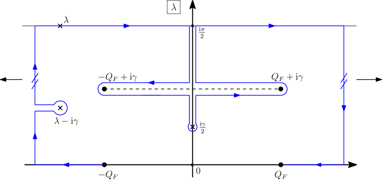
Figure 2: We deform the original integration contour, which is a straight line from $-Q_{F}$ to $Q_{F}$ to the sketched contour and move the left and the right parts to minus and plus infinity.

Directly from the defining integral equation we can read off the following properties of the dressed energy in the strip $0<{\rm Im\,}\lambda<\frac{\pi}{2}$.

1. $\varepsilon$ has a simple pole at $\lambda={\rm i}\frac{\gamma}{2}$ with residue

   $$\operatorname{res}_{\lambda={\rm i}\frac{\gamma}{2}}\varepsilon(\lambda)=2{\rm i}J\sin(\gamma)\,.$$ (70)

2. $\varepsilon$ has a jump discontinuity across the cut at $[-Q_{F},Q_{F}]+{\rm i}\gamma$, where

   $$\varepsilon_{+}(\lambda)-\varepsilon_{-}(\lambda)=\varepsilon(\lambda-{\rm i}\gamma)\,.$$ (71)

3. $$\lim_{{\rm Re\,}\lambda\rightarrow\pm\infty}\varepsilon(\lambda)=h\,.$$ (72)

We now first of all choose $\lambda$ such that ${\rm Im\,}\lambda=\frac{\pi}{2}$. Evaluating the integral that occurs in the integral equation for $\varepsilon$ along the original contour and along the deformed contour and using the above properties and the properties of the kernel we obtain the identity

$$\int_{-Q_{F}}^{Q_{F}} {\rm d}\mu\>K(\lambda-\mu|\gamma)\varepsilon(\mu)$$

$$=-\varepsilon(\lambda-{\rm i}\gamma)-4\pi J\sin(\gamma)K(\lambda-{\rm i}\gamma/2|\gamma)-\int_{-Q_{F}}^{Q_{F}}{\rm d}\mu\>K(\lambda-\mu-{\rm i}\gamma|\gamma)\varepsilon(\mu)$$

$$\mspace{36.0mu}+\int_{{\mathbb{R}}+{\rm i}\frac{\pi}{2}}{\rm d}\mu\>K(\lambda-\mu|\gamma)\varepsilon(\mu)-\int_{{\mathbb{R}}\setminus[-Q_{F},Q_{F}]}{\rm d}\mu\>K(\lambda-\mu|\gamma)\varepsilon(\mu)$$

$$=-\varepsilon_{0}(\lambda-{\rm i}\gamma)-4\pi J\sin(\gamma)K(\lambda-{\rm i}\gamma/2|\gamma)$$

$$\mspace{36.0mu}+\int_{{\mathbb{R}}+{\rm i}\frac{\pi}{2}}{\rm d}\mu\>K(\lambda-\mu|\gamma)\varepsilon(\mu)-\int_{{\mathbb{R}}\setminus[-Q_{F},Q_{F}]}{\rm d}\mu\>K(\lambda-\mu|\gamma)\varepsilon(\mu)\,.$$ (73)

We insert this into the defining integral equation for $\varepsilon$ and combine the explicit terms on the right hand side of (3.2) with the driving term. It follows that

$$\varepsilon(\lambda)=2h-\int_{{\mathbb{R}}+{\rm i}\frac{\pi}{2}}{\rm d}\mu\>K(\lambda-\mu|\gamma)\varepsilon(\mu)+\int_{{\mathbb{R}}\setminus[-Q_{F},Q_{F}]}{\rm d}\mu\>K(\lambda-\mu|\gamma)\varepsilon(\mu)\,.$$ (74)

We set $\lambda=z+{\rm i}\frac{\pi}{2}$ and

$$\omega(z)=\varepsilon(z+{\rm i}\pi/2)\,.$$ (75)

Then, using the ${\rm i}\pi$-periodicity of the kernel, (74) turns into

$$\omega(z)=2h-\int_{{\mathbb{R}}\setminus[-Q_{F},Q_{F}]}{\rm d}w\>K(z-w|\pi/2-\gamma)\varepsilon(w)-\int_{-\infty}^{\infty}{\rm d}w\>K(z-w|\gamma)\omega(w)\,.$$ (76)

This equation can be solved for $\omega$ by employing Fourier transformation and the convolution theorem. For $\lambda\in{\mathbb{R}}$ let

$$\varepsilon_{c}(\lambda)=\begin{cases}\varepsilon(\lambda)&\text{if $\lambda\in{\mathbb{R}}\setminus[-Q_{F},Q_{F}]$}\\ 0&\text{else.}\end{cases}$$ (77)

Then

$${\cal F}[\omega](k)=\frac{2\pi h\,\delta(k)}{1-\frac{\gamma}{\pi}}-{\cal F}[D](k){\cal F}[\varepsilon_{c}](k)\,,$$ (78)

where

$${\cal F}[D](k)=\frac{\operatorname{sh}\bigl{(}\frac{\gamma k}{2}\bigr{)}}{\operatorname{sh}\bigl{(}(\pi-\gamma)\frac{k}{2}\bigr{)}}\,.$$ (79)

It follows that

$$D(z)=\frac{K\Bigl{(}\frac{z}{1-\frac{\gamma}{\pi}}\Big{|}\frac{\pi}{2}-\gamma^{\prime}\Bigr{)}}{1-\frac{\gamma}{\pi}}$$ (80)

with $\gamma^{\prime}$ as defined in (30). Hence, $\omega$ has the representation

$$\omega(z)=\frac{h}{1-\frac{\gamma}{\pi}}-\frac{1}{1-\frac{\gamma}{\pi}}\int_{{\mathbb{R}}\setminus[-Q_{F},Q_{F}]}{\rm d}w\>K\biggl{(}\frac{z-w}{1-\frac{\gamma}{\pi}}\bigg{|}\frac{\pi}{2}-\gamma^{\prime}\biggr{)}\varepsilon(w)\,.$$ (81)

Recall that $\gamma\mapsto\gamma^{\prime}$ is a monotonically increasing bijection of the interval $(0,\pi/2)$. Hence, $\gamma\mapsto\frac{\pi}{2}-\gamma^{\prime}$ is a monotonically decreasing function that maps $(0,\pi/2)$ onto itself. Further notice that the kernel in (81) as a function of $z-w$ has simple poles at $\pm{\rm i}\bigl{(}\frac{\pi}{2}-\gamma\bigr{)}\mod{\rm i}(\pi-\gamma)$.

We shall use (81) to establish the lower bounds (19a) and (19b). Let us begin with (19a). Since $K$ is harder to estimate than $R$ we use the integral equation (28) in order to replace the kernel function $K$ on the right hand side of (81). Setting $x={\rm Re\,}z={\rm Re\,}\lambda$, $b={\rm Im\,}z={\rm Im\,}\lambda-\pi/2=y-\pi/2$ and taking the real part and the $x$-derivative of (81) we arrive after a few elementary manipulations at

$$\partial_{x}{\rm Re\,}\omega(z)= -\frac{1}{1-\frac{\gamma}{\pi}}\int_{Q_{F}}^{\infty}{\rm d}w\>{\rm Re\,}\biggl{\{}R\biggl{(}\frac{z-w}{1-\frac{\gamma}{\pi}}\bigg{|}\frac{\pi}{2}-\gamma^{\prime}\biggr{)}-R\biggl{(}\frac{z+w}{1-\frac{\gamma}{\pi}}\bigg{|}\frac{\pi}{2}-\gamma^{\prime}\biggr{)}\biggr{\}}\varepsilon^{\prime}(w)$$

$$\mspace{-90.0mu}-\frac{1}{\bigl{(}1-\frac{\gamma}{\pi}\bigr{)}^{2}}\int_{0}^{\infty}{\rm d}w\>{\rm Re\,}\biggl{\{}R\biggl{(}\frac{z-w}{1-\frac{\gamma}{\pi}}\bigg{|}\frac{\pi}{2}-\gamma^{\prime}\biggr{)}-R\biggl{(}\frac{z+w}{1-\frac{\gamma}{\pi}}\bigg{|}\frac{\pi}{2}-\gamma^{\prime}\biggr{)}\biggr{\}}$$

$$\mspace{-18.0mu}\times\int_{Q_{F}}^{\infty}{\rm d}u\>{\rm Re\,}\biggl{\{}K\biggl{(}\frac{w-u}{1-\frac{\gamma}{\pi}}\bigg{|}\frac{\pi}{2}-\gamma^{\prime}\biggr{)}-K\biggl{(}\frac{w+u}{1-\frac{\gamma}{\pi}}\bigg{|}\frac{\pi}{2}-\gamma^{\prime}\biggr{)}\biggr{\}}\varepsilon^{\prime}(u)\,.$$ (82)

Now (63) implies that

$${\rm Re\,}\biggl{\{}R\biggl{(}\frac{z-w}{1-\frac{\gamma}{\pi}}\bigg{|}\frac{\pi}{2}-\gamma^{\prime}\biggr{)}-R\biggl{(}\frac{z+w}{1-\frac{\gamma}{\pi}}\bigg{|}\frac{\pi}{2}-\gamma^{\prime}\biggr{)}\biggr{\}}>0$$ (83)

for all $x={\rm Re\,}z>0$, $w>0$ if

$$|b|<\biggl{(}1-\frac{\gamma}{\pi}\biggr{)}\frac{1}{2}\biggl{(}\frac{\pi}{2}-\gamma^{\prime}\biggr{)}=\frac{1}{2}\biggl{(}\frac{\pi}{2}-\gamma\biggr{)}\,.$$ (84)

Since $\varepsilon^{\prime}(w)>0$ for $w>0$ and since the same is true for the difference of the kernel functions $K$ in the second integral on the right hand side of (3.2) we conclude that $\partial_{x}{\rm Re\,}\omega(z)<0$, meaning that $x\mapsto{\rm Re\,}\omega(x+{\rm i}b)$ is monotonically decreasing on ${\mathbb{R}}_{+}$ if $b$ satisfies (84). Thus, $x\mapsto{\rm Re\,}\varepsilon(x+{\rm i}y)$ is monotonically decreasing on ${\mathbb{R}}_{+}$ for $\frac{\pi}{2}-\frac{1}{2}\bigl{(}\frac{\pi}{2}-\gamma\bigr{)}<y<\frac{\pi}{2}$. Combining this knowledge with the asymptotic formula (72) we have established (19a).

Proof of (19b)

We proceed with (19b). For the proof we consider (81) with

$$\gamma-\frac{\pi}{2}<b={\rm Im\,}z<\frac{1}{2}\biggl{(}\gamma-\frac{\pi}{2}\biggr{)}<0\,.$$ (85)

Equation (23) implies that

$${\rm Re\,}K\biggl{(}\frac{z-w}{1-\frac{\gamma}{\pi}}\bigg{|}\frac{\pi}{2}-\gamma^{\prime}\biggr{)}=\frac{1}{2}\biggl{\{}K\biggl{(}\frac{x-w}{1-\frac{\gamma}{\pi}}\bigg{|}\gamma_{+}\biggr{)}+K\biggl{(}\frac{x-w}{1-\frac{\gamma}{\pi}}\bigg{|}\gamma_{-}\biggr{)}\biggr{\}}\,,$$ (86)

where $x={\rm Re\,}z$ and

$$\gamma_{\pm}=\frac{\pi}{2}-\gamma^{\prime}\pm\frac{b}{1-\frac{\gamma}{\pi}}\,.$$ (87)

The inequality (85) implies that

$$0<\gamma_{+}<\frac{\pi}{4}\,,\quad\gamma_{+}<\gamma_{-}<\pi\,.$$ (88)

Hence, we have to distinguish two cases, $\gamma_{-}<\frac{\pi}{2}$ or $\gamma_{-}>\frac{\pi}{2}$.

Taking the real part and the $x$-derivative of (81) we see that

$$\partial_{x}{\rm Re\,}\omega(z)=-\frac{1}{1-\frac{\gamma}{\pi}}\int_{Q_{F}}^{\infty}{\rm d}w\>\sum_{\sigma=\pm}\biggl{\{}K\biggl{(}\frac{x-w}{1-\frac{\gamma}{\pi}}\bigg{|}\gamma_{\sigma}\biggr{)}-K\biggl{(}\frac{x+w}{1-\frac{\gamma}{\pi}}\bigg{|}\gamma_{\sigma}\biggr{)}\biggr{\}}\frac{\varepsilon^{\prime}(w)}{2}\,.$$ (89)

If $\gamma_{-}<\frac{\pi}{2}$, then the summands for $\sigma=+$ and for $\sigma=-$ are both positive. Since moreover $\varepsilon^{\prime}(w)>0$ for $w>0$, we conclude that $x\mapsto{\rm Re\,}\omega(x+{\rm i}b)$ is monotonically decreasing on ${\mathbb{R}}_{+}$. Thus, (72) implies that ${\rm Re\,}\omega(x+{\rm i}b)>h$ in this case.

On the other hand, if $\gamma_{-}>\frac{\pi}{2}$, then $K(x/(1-\gamma/\pi)|\gamma_{-})<0$ for all $x\in{\mathbb{R}}$ and

$${\rm Re\,}\omega(z)>\frac{h}{1-\frac{\gamma}{\pi}}-\frac{1}{1-\frac{\gamma}{\pi}}\int_{{\mathbb{R}}\setminus[-Q_{F},Q_{F}]}{\rm d}w\>K\biggl{(}\frac{x-w}{1-\frac{\gamma}{\pi}}\bigg{|}\gamma_{+}\biggr{)}\frac{\varepsilon(w)}{2}=F(x)\,.$$ (90)

As above we can conclude that $F^{\prime}(x)<0$ for all $x>0$. For the asymptotic behaviour of this function we obtain

$$\lim_{x\rightarrow\infty}F(x)=\frac{h}{1-\frac{\gamma}{\pi}}-\frac{h}{2}\int_{-\infty}^{\infty}{\rm d}w\>K(w|\gamma_{+})\\ =\frac{h}{1-\frac{\gamma}{\pi}}-\frac{h}{\pi}\biggl{(}\gamma^{\prime}-\frac{b}{1-\frac{\gamma}{\pi}}\biggr{)}>\frac{h}{2}\frac{1+\frac{\gamma}{\pi}}{1-\frac{\gamma}{\pi}}>\frac{h}{2}\,.$$ (91)

Thus, ${\rm Re\,}\omega(z)>\frac{h}{2}$, whenever (85) is satisfied, or ${\rm Re\,}\varepsilon(x+{\rm i}y)>\frac{h}{2}$ for all $x\in{\mathbb{R}}$ if $\gamma<y<\frac{\pi}{2}-\frac{1}{2}\bigl{(}\frac{\pi}{2}-\gamma\bigr{)}$, which is (19b).

Proof of (19c)

It remains to prove (19c). For this purpose we start with (44) for the dressed energy,

$$\varepsilon(\lambda)=\varepsilon_{\infty}(\lambda)+\int_{{\mathbb{R}}\setminus[-Q_{F},Q_{F}]}{\rm d}\mu\>R(\lambda-\mu|\gamma)\varepsilon(\mu)\,.$$ (92)

First of all equation (61a) with $\frac{\gamma}{2}<y<\gamma$ implies that

$${\rm Re\,}\varepsilon_{\infty}(\lambda)>\frac{h}{2\bigl{(}1-\frac{\gamma}{\pi}\bigr{)}}\,.$$ (93)

In order to estimate the real part of the integral in (92), we define the function

$$R_{I}(\lambda|\gamma)=\frac{\pi}{2\gamma(\pi-\gamma)}\int_{-\infty}^{\infty}{\rm d}\mu\>\frac{K\Bigl{(}\frac{\mu}{1-\frac{\gamma}{\pi}}\Big{|}\frac{\gamma/2}{1-\frac{\gamma}{\pi}}\Bigr{)}}{\operatorname{ch}\bigl{(}(\lambda-\mu)\frac{\pi}{\gamma}\bigr{)}}$$ (94)

which, for $\frac{\gamma}{2}<y={\rm Im\,}\lambda<\gamma$ differs from the resolvent $R(\lambda|\gamma)$. Analytically continuing (27) we rather see that

$$R(\lambda|\gamma)=R_{I}(\lambda|\gamma)+\frac{1}{1-\frac{\gamma}{\pi}}K\biggl{(}\frac{\lambda-{\rm i}\gamma/2}{1-\frac{\gamma}{\pi}}\bigg{|}\frac{\gamma/2}{1-\frac{\gamma}{\pi}}\biggr{)}\,.$$ (95)

Hence,

$$\int_{{\mathbb{R}}\setminus[-Q_{F},Q_{F}]}{\rm d}\mu\>{\rm Re\,}\bigl{(}R(\lambda-\mu|\gamma)\bigr{)}\varepsilon(\mu)=\int_{{\mathbb{R}}\setminus[-Q_{F},Q_{F}]}{\rm d}\mu\>{\rm Re\,}\bigl{(}R_{I}(\lambda-\mu|\gamma)\bigr{)}\varepsilon(\mu)\\[4.30554pt] \mspace{-1.0mu}+\frac{1}{2\bigl{(}1-\frac{\gamma}{\pi}\bigr{)}}\int_{{\mathbb{R}}\setminus[-Q_{F},Q_{F}]}{\rm d}\mu\>\biggl{\{}K\biggl{(}\frac{x-\mu}{1-\frac{\gamma}{\pi}}\bigg{|}\frac{\gamma-y}{1-\frac{\gamma}{\pi}}\biggr{)}+K\biggl{(}\frac{x-\mu}{1-\frac{\gamma}{\pi}}\bigg{|}\frac{y}{1-\frac{\gamma}{\pi}}\biggr{)}\biggr{\}}\varepsilon(\mu)\,.$$ (96)

Now ${\rm Re\,}R_{I}(\lambda-\mu)<0$ for all $y={\rm Im\,}\lambda\in(\gamma/2,\gamma)$, $x={\rm Re\,}\lambda,\mu\in{\mathbb{R}}$, because of (61a), (94), while $0<\varepsilon(\mu)<h$ for all $\mu\in{\mathbb{R}}\setminus[-Q_{F},Q_{F}]$. Thus,

$$\int_{{\mathbb{R}}\setminus[-Q_{F},Q_{F}]}{\rm d}\mu\>{\rm Re\,}\bigl{(}R_{I}(\lambda-\mu|\gamma)\bigr{)}\varepsilon(\mu)$$

$$\mspace{18.0mu}>h\int_{{\mathbb{R}}\setminus[-Q_{F},Q_{F}]}{\rm d}\mu\>{\rm Re\,}\bigl{(}R_{I}(\lambda-\mu|\gamma)\bigr{)}>h\int_{-\infty}^{\infty}{\rm d}\mu\>{\rm Re\,}\bigl{(}R_{I}(\mu-{\rm i}y|\gamma)\bigr{)}$$

$$\mspace{18.0mu}=\frac{h}{2\gamma\bigl{(}1-\frac{\gamma}{\pi}\bigr{)}}\int_{-\infty}^{\infty}{\rm d}\nu\>K\Bigl{(}\frac{\nu}{1-\frac{\gamma}{\pi}}\Big{|}\frac{\gamma/2}{1-\frac{\gamma}{\pi}}\Bigr{)}{\rm Re\,}\int_{-\infty}^{\infty}{\rm d}\mu\>\frac{1}{\operatorname{ch}\bigl{(}(\mu-\nu-{\rm i}y)\frac{\pi}{\gamma}\bigr{)}}$$

$$\mspace{18.0mu}=-\frac{h}{2}\frac{1-\frac{2\gamma}{\pi}}{1-\frac{\gamma}{\pi}}\,.$$ (97)

Here we have used the residue theorem and equation (24) to evaluate the integrals in the last equation.

In order to estimate the second integral in (96) we note that $\frac{\gamma}{2}<y<\gamma$ implies that

$$0<\frac{\gamma-y}{1-\frac{\gamma}{\pi}}<\gamma^{\prime}<\frac{y}{1-\frac{\gamma}{\pi}}<2\gamma^{\prime}\,.$$ (98)

Recalling that $0<\gamma^{\prime}<\frac{\pi}{2}$ we see that the contribution of the first kernel to the second integral in (96) is always positive. Hence,

$$\frac{1}{2\bigl{(}1-\frac{\gamma}{\pi}\bigr{)}}\int_{{\mathbb{R}}\setminus[-Q_{F},Q_{F}]}{\rm d}\mu\>\biggl{\{}K\biggl{(}\frac{x-\mu}{1-\frac{\gamma}{\pi}}\bigg{|}\frac{\gamma-y}{1-\frac{\gamma}{\pi}}\biggr{)}+K\biggl{(}\frac{x-\mu}{1-\frac{\gamma}{\pi}}\bigg{|}\frac{y}{1-\frac{\gamma}{\pi}}\biggr{)}\biggr{\}}\varepsilon(\mu)$$

$$\mspace{18.0mu}>\frac{1}{2\bigl{(}1-\frac{\gamma}{\pi}\bigr{)}}\int_{{\mathbb{R}}\setminus[-Q_{F},Q_{F}]}{\rm d}\mu\>K\biggl{(}\frac{x-\mu}{1-\frac{\gamma}{\pi}}\bigg{|}\frac{y}{1-\frac{\gamma}{\pi}}\biggr{)}\varepsilon(\mu)$$

$$\mspace{18.0mu}>\begin{cases}0&\text{if $\frac{y}{1-\frac{\gamma}{\pi}}<\frac{\pi}{2}$}\\[4.30554pt] \frac{h}{2}\frac{1-\frac{3\gamma}{\pi}}{1-\frac{\gamma}{\pi}}&\text{if $\frac{y}{1-\frac{\gamma}{\pi}}>\frac{\pi}{2}$.}\end{cases}$$ (99)

For the second case in the last line we have estimated the integral by replacing $\varepsilon(\mu)$ by $h$ and the range of integration by the real axis as in (3.2). Combining the estimates (93), (3.2) and (3.2) we arrive at the conclusion that

$${\rm Re\,}\varepsilon(\lambda)>\begin{cases}\frac{h\gamma}{\pi-\gamma}&\text{if $y<\frac{\pi}{2}-\frac{\gamma}{2}$}\\[4.30554pt] \frac{h}{2}&\text{if $y>\frac{\pi}{2}-\frac{\gamma}{2}$}\end{cases}$$ (100)

which entails the claim (19c).

Proof of (vi) and (vii)

(vi) is a consequence of an analogous property of the kernel function $K(\cdot|\gamma)$. In order to show (vii) we introduce the notation $u={\rm Re\,}\varepsilon$, $v={\rm Im\,}\varepsilon$, $x={\rm Re\,}\lambda$, $y={\rm Im\,}\lambda$ and consider $\lambda$ as $\lambda(y)=x(y)+{\rm i}y$. The curve $u(\lambda)=0$ is located in the strip $|y|<\gamma/2$. In this strip $u_{x}>0$ according to (ii). By implicit differentiation

$$\frac{{\rm d}x}{{\rm d}y}=-\frac{u_{y}}{u_{x}}\,.$$ (101)

It follows that

$$\frac{{\rm d}v}{{\rm d}y}=v_{x}\frac{{\rm d}x}{{\rm d}y}+v_{y}=-\frac{v_{x}u_{y}}{u_{x}}+v_{y}=\frac{v_{x}^{2}}{u_{x}}+u_{x}>0\,.$$ (102)

Here we have used the Cauchy-Riemann equations in the third equation. Equation (21) is obtained by inserting (16) into the leading term of the Laurent expansion of $\varepsilon$ obtained, for instance, from the integral equation (4) with $f_{0}=\varepsilon_{0}$, $Q=Q_{F}$.

4 Conclusions

We have studied some of the properties of the dressed energy $\varepsilon$ of the XXZ chain in the complex plane. In particular, we have obtained a clear picture of where ${\rm Re\,}\varepsilon$ is positive and where it is negative. Both regions are separated by the smooth simple and closed curve ${\rm Re\,}\varepsilon=0$, which is reflection symmetric with respect to real and imaginary axis, which goes through two Fermi points $\pm Q_{F}$ on the real axis and through the points $\pm{\rm i}\gamma/2$. Moreover, this curve is entirely located inside the strip ${\rm Im\,}\lambda\leq\gamma/2$. In the right half plane ${\rm Im\,}\varepsilon$ is monotonically increasing in the direction of increasing imaginary part and is diverging at $\pm{\rm i}\gamma/2$. These properties are essential for a future rigorous characterization of the auxiliary functions that determine the sets of Bethe roots and the eigenvalues of the quantum transfer matrix of the model in the zero-temperature limit.

Acknowledgments. The authors would like to thank Junji Suzuki for a critical reading of the manuscript and for his valuable comments. SF and FG acknowledge financial support by the DFG in the framework of the research unit FOR 2316. The work of KKK is supported by the CNRS and by the ‘Projet international de coopération scientifique No. PICS07877’: Fonctions de corrélations dynamiques dans la chaîne XXZ à température finie, Allemagne, 2018-2020.

References

- [1] C. Babenko, F. Göhmann, K. K. Kozlowski, and J. Suzuki, A thermal form factor series for the longitudinal two-point function of the Heisenberg-Ising chain in the antiferromagnetic massive regime, J. Math. Phys. 62 (2021), 041901.
- [2] H. Bethe, Zur Theorie der Metalle. I. Eigenwerte und Eigenfunktionen der linearen Atomkette, Z. Phys. 71 (1931), 205–226.
- [3] M. Dugave, F. Göhmann, and K. K. Kozlowski, Thermal form factors of the XXZ chain and the large-distance asymptotics of its temperature dependent correlation functions, J. Stat. Mech.: Theor. Exp. (2013), P07010.
- [4] , Functions characterizing the ground state of the XXZ spin- chain in the thermodynamic limit, SIGMA 10 (2014), 043.
- [5] , Low-temperature large-distance asymptotics of the transversal two-point functions of the XXZ chain, J. Stat. Mech.: Theor. Exp. (2014), P04012.
- [6] M. Dugave, F. Göhmann, K. K. Kozlowski, and J. Suzuki, Low-temperature spectrum of correlation lengths of the XXZ chain in the antiferromagnetic massive regime, J. Phys. A 48 (2015), 334001.
- [7] , Thermal form factor approach to the ground-state correlation functions of the XXZ chain in the antiferromagnetic massive regime, J. Phys. A 49 (2016), 394001.
- [8] I. Gohberg, S. Goldberg, and N. Krupnik, Traces and determinants of linear operators, Operator Theory – Advances and Applications, vol. 116, Birkhäuser Verlag, Basel, 2000.
- [9] F. Göhmann, M. Karbach, A. Klümper, K. K. Kozlowski, and J. Suzuki, Thermal form-factor approach to dynamical correlation functions of integrable lattice models, J. Stat. Mech.: Theor. Exp. (2017), 113106.
- [10] N. Kitanine, K. K. Kozlowski, J. M. Maillet, N. A. Slavnov, and V. Terras, A form factor approach to the asymptotic behavior of correlation functions in critical models, J. Stat. Mech.: Theor. Exp. (2011), P12010.
- [11] N. Kitanine, J. M. Maillet, and V. Terras, Correlation functions of the XXZ Heisenberg spin- chain in a magnetic field, Nucl. Phys. B 567 (2000), 554.
- [12] A. Klümper, Free energy and correlation length of quantum chains related to restricted solid-on-solid lattice models, Ann. Physik 1 (1992), 540.
- [13] R. Orbach, Linear antiferromagnetic chain with anisotropic coupling, Phys. Rev. 112 (1958), 309.
- [14] E. K. Sklyanin, L. A. Takhtadzhyan, and L. D. Faddeev, Quantum inverse problem method. I., Theor. Math. Phys. 40 (1979), 688.
- [15] J. Suzuki, Y. Akutsu, and M. Wadati, A new approach to quantum spin chains at finite temperature, J. Phys. Soc. Jpn. 59 (1990), 2667.
- [16] M. Suzuki, Transfer-matrix method and Monte Carlo simulation in quantum spin systems, Phys. Rev. B 31 (1985), 2957.
- [17] M. Takahashi and M. Suzuki, One-dimensional anisotropic Heisenberg model at finite temperatures, Prog. Theor. Phys. 48 (1972), 2187.
- [18] L. R. Walker, Antiferromagnetic linear chain, Phys. Rev. 116 (1959), 1089.
- [19] C. N. Yang and C. P. Yang, Ground-state energy of a Heisenberg-Ising lattice, Phys. Rev. 147 (1966), 303.
- [20] , One-dimensional chain of anisotropic spin-spin interactions. I. Proof of Bethe’s hypothesis for ground state in a finite system, Phys. Rev. 150 (1966), 321.
- [21] , One-dimensional chain of anisotropic spin-spin interactions. II. Properties of the ground-state energy per lattice site for an infinite system, Phys. Rev. 150 (1966), 327.
- [22] , Thermodynamics of a one-dimensional system of Bosons with repulsive delta-function interaction, J. Math. Phys. 10 (1969), 1115.