TDGIA: Effective Injection Attacks on Graph Neural Networks

Abstract.

Graph Neural Networks (GNNs) have achieved promising performance in various real-world applications. However, recent studies find that GNNs are vulnerable to adversarial attacks. In this paper, we study a recently-introduced realistic attack scenario on graphs—graph injection attack (GIA). In the GIA scenario, the adversary is not able to modify the existing link structure or node attributes of the input graph, instead the attack is performed by injecting adversarial nodes into it. We present an analysis on the topological vulnerability of GNNs under GIA setting, based on which we propose the Topological Defective Graph Injection Attack (TDGIA) for effective injection attacks. TDGIA first introduces the topological defective edge selection strategy to choose the original nodes for connecting with the injected ones. It then designs the smooth feature optimization objective to generate the features for the injected nodes. Extensive experiments on large-scale datasets show that TDGIA can consistently and significantly outperform various attack baselines in attacking dozens of defense GNN models. Notably, the performance drop on target GNNs resultant from TDGIA is more than double the damage brought by the best attack solution among hundreds of submissions on KDD-CUP 2020.

1. Introduction

Recent years have witnessed widespread adoption of graph machine learning for modeling structured and relational data. Particularly, the emergence of graph neural networks (GNNs) has offered promising results in diverse graph applications, such as node classification (Kipf and Welling, 2016), social recommendation (Ying et al., 2018), and drug design (Jiang et al., 2020).

Despite the exciting progress, studies have shown that neural networks are commonly vulnerable to adversarial attacks, where slight, imperceptible but intentionally-designed perturbations on inputs can cause incorrect predictions (Szegedy et al., 2013; Goodfellow et al., 2014a; Huang et al., 2017). Attacks on general neural networks usually focus on modifying the attributes/features of the input instances, such as minor perturbations in individual pixels of an image. Uniquely, adversarial attacks can also be applied to graph-structured input, requiring dedicated strategies for exploring the specific vulnerabilities of the underlying models.

The early attacks on GNNs usually follow the setting of graph modification attack (GMA) (Dai et al., 2018; Zügner et al., 2018; Sun et al., 2020; Zügner and Günnemann, 2019), as illustrated in Figure 1 (a): given an input graph with attributes, the adversary can directly modify the links between its nodes (red links) and the attributes of existing nodes (red nodes). However, in real-world scenarios, it is often unrealistic for the adversary to get the authority to modify existing data. Take the citation graph for example, it automatically forms when papers are published, making it practically difficult to change the citations and attributes of one publication afterwards. But what is relatively easy is to inject new nodes and links into the existing citation graph, e.g., by “publishing” fake papers, to mislead the predictions of GNNs.

In view of the gap, very recent efforts (Sun et al., 2020; Wang et al., 2020), including the KDD-CUP 2020 competition, have been devoted to adversarial attacks on GNNs under the setting of graph injection attack (GIA). Specifically, the GIA task in KDD-CUP 2020 is formulated as follows: (1) Black-box attack, where the adversaries do not have access to the target GNN model or the correct labels of the target nodes; (2) Evasion attack, where the attacks can only be performed during the inference stage. The GIA settings present unique challenges that are not faced by GMA, such as how to connect existing nodes with injected nodes and how to generate features for injected nodes from scratch. Consequently, though numerous attacks are submitted by hundreds of teams, the resultant performance drops are relatively limited and no principled models emerge from them.

    

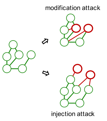
(a) GMA vs. GIA

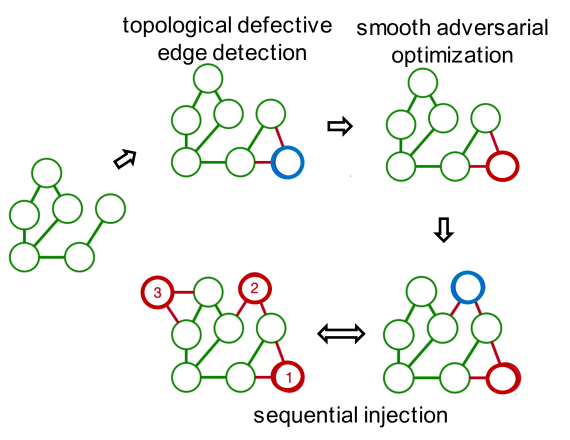
(b) Topological Defective Graph Injection Attack (TDGIA)

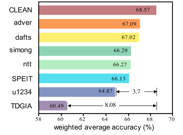
(c) TDGIA vs. The Best Results in KDD-CUP 2020

Figure 1. An overview of graph injection attack, the proposed TDGIA method, and its performance.

Contributions. In this work, we study the problem of GIA under the black-box and evasion attack settings, where the goal is to design an effective injection attack framework that can best fool the target GNN models and thus worsen their prediction capability. To understand the problem and its challenges, we present an in-depth analysis of the vulnerability of GNNs under the graph injection attack and show that GNNs, as non-structural-ignorant models, are GIA-attackable. Based on this, we present the topological defective graph injection attack (TDGIA) (Cf. Figure 1 (b)). TDGIA consists of two modules—topological defective edge selection and smooth adversarial optimization for injected node attribute generation—that corresponds to the problem setup of GIA. Specifically, we leverage the topological vulnerabilities of the original graph to detect existing nodes that can best help the attack and then inject new nodes surrounding them in a sequential manner. With that, we design a smooth loss function to optimize the nodes’ features for minimizing the the performance of the target GNN model.

Both the studied problem and the proposed TDGIA method differ from existing (injection) attack methods. Table 1 summarizes the differences. First, NIPA (Sun et al., 2020) and AFGSM (Wang et al., 2020) are developed under the poison setting, which requires the re-training of the defense models for each attack. Differently, TDGIA follows KDD-CUP 2020 to use the evasion attack setting, where different attacks are evaluated based on the same set of models and weights. Second, the design of TDGIA enables it to attack large-scale graphs that can not be handled by the reinforcement-learning based NIPA. Third, compared with AFGSM, TDGIA proposes a more general way to consume the topological information, resulting in significant performance improvements. Finally, attacks in previous works are only evaluated on weak defense models like raw GCN, while TDGIA is shown to be effective even against the top defense solutions examined in KDD-CUP 2020.

We conduct extensive experiments on large-scale datasets to demonstrate the performance and transferability of the proposed attack method. Figure 1 (c) lists the results for TDGIA and the top submissions on KDD-CUP 2020 as measured by weighted average accuracy. The experimental results show that TDGIA significantly and consistently outperforms various baseline methods. For example, the best KDD-CUP 2020 attack (u1234) can make the performance of the target GNN models drop $3.7\%$, while TDGIA can drag its performance down by $8.08\%$—a $118\%$ increase in damage. Moreover, TDGIA achieves this attack performance by injecting only a limited number of nodes ($1\%$ of target nodes). Additionally, various ablation studies demonstrate the effectiveness of each module in TDGIA.

To sum up, this work makes the following contributions:

• We study the GIA problem with the black-box and evasion settings, and theoretically show that non-structural-ignorant GNN models are vulnerable to GIA.

• We develop the Topological Defective Graph Injection Attack (TDGIA) that can explore and leverage the vulnerability of GNNs and the topological properties of the graph.

• We conduct experiments that consistently demonstrate TDGIA’s significant outperformance over baselines (including the best attack submission at KDD-CUP 2020) against various defense GNN models across different datasets.

Table 1. Summary of graph adversarial attacks.

Attack	Task	Type	Method	Attack Setting
Dai et al. (Dai et al., 2018)	Node cl. Graph cl.	GMA	Reinforcement learning	Evasion
Nettack (Zügner et al., 2018)	Node cl. Graph cl.	GMA	Greedy algorithm Model linearization	Evasion Poison
Meta (Zügner and Günnemann, 2019)	Node cl.	GMA	Meta-learning	Poison
NIPA (Sun et al., 2020)	Node cl.	GIA	Reinforcement learning	Poison
AFGSM (Wang et al., 2020)	Node cl.	GIA	Fast Gradient Sign Model linearization	Poison
TDGIA (ours)	Node cl.	GIA	Defective edge selection Smooth optimization	Evasion

2. Related Works

Adversarial Attacks on Neural Networks. The phenomenon of adversarial examples against deep-learning based models is first discovered in computer vision (Szegedy et al., 2013). Adding delicate and imperceptible perturbations to images can significantly change the predictions of deep neural networks.  (Goodfellow et al., 2014b) proposes Fast Gradient Sign Method (FGSM) to generate this kind of perturbations by using the gradients of trained neural networks. Since then, more advanced attack methods are proposed (Carlini and Wagner, 2017; Athalye et al., 2018). Adversarial attacks also grow in a wider range of fields such as natural language processing (Li et al., 2019), or speech recognition (Carlini and Wagner, 2018). Nowadays, adversarial attacks have become one of the major threats to neural networks.

Adversarial Attacks on GNNs. Due to the existence of adversarial examples, the vulnerability of graph learning algorithms has also been revealed. By modifying features and edges on graph-structured data, the adversary can significantly degrade the performance of GNN models. As shown in Table 1,  (Dai et al., 2018) proposes a reinforcement-learning based attack on both node classification and graph classification tasks. This attack only modifies the structure of graph.  (Zügner et al., 2018) proposes Nettack, the first adversarial attack on attributed graphs. It shows that only few perturbations on both edges and features of the graph can be extremely harmful for models like GCN. Nettack uses a greedy approximation scheme under the constraints of unnoticeable perturbations and incorporates fast computation. Furthermore,  (Zügner and Günnemann, 2019) proposes a poison attack on GNNs via meta-learning, Meta-attack, which only modifies a small part of the graph but can still decrease the performance of GNNs on node classification tasks remarkably. A recent summary (Jin et al., 2021) summarizes different graph adversarial attacks.

A more realistic scenario, graph injection attack (GIA), is studied in (Sun et al., 2020; Wang et al., 2020), which injects new vicious nodes instead of modifying the original graph.  (Sun et al., 2020) proposes Node Injection Poisoning Attack (NIPA) based on reinforcement learning strategy. Under the same scenario, Approximate Fast Gradient Sign Method (AFGSM) (Wang et al., 2020) further uses an approximation strategy to linearize the model and to generate the perturbations efficiently. These works are under the poison setting, where models have to be re-trained after the vicious nodes are injected onto the graph.

KDD-CUP 2020 Graph Adversarial Attack & Defense. KDD-CUP 2020 introduces the GIA scenario in Graph Adversarial Attack & Defense competition track. The adversary doesn’t have access to the target model (i.e. black-box setting), and can only inject no more than 500 nodes to a large citation network with more than 600,000 nodes and millions of links.

For attackers, the attack is conducted during the inference stage, a.k.a. the evasion setting. For defenders, they should provide robust GNN models to resist various adversarial attacks. Hundreds of attack and defense solutions are submitted during the competition, which serve as good references for further development of graph adversarial attacks.

Another similar setting is introduced in KDD-CUP 2020. The Graph Adversarial Attack & Defense Track introduced a setting that the injection nodes are injected only during the inference stage. To separate this setting from the poison attack setting, we call this evasion attack.

Table 2. Summary of several adversarial attacks on Graph Neural Networks.

Attacks	Task	Modification	Methodology	Attack Stage
Dai et al. (Dai et al., 2018)	Node classification, Graph classification	Edges	Reinforcement learning	Evasion attack
Nettack (Zügner et al., 2018)	Node classification. Graph classification	Edges & Features	Greedy algorithm, Model linearization	Evasion attack, Poisoning attack
Meta-attack (Zügner and Günnemann, 2019)	Node classification	Edges & Features	Meta-learning	Poison attack
NIPA (Sun et al., 2020)	Node classification	Node injection	Reinforcement learning	Poison attack
AFGSM (Wang et al., 2020)	Node classification	Node injection	Fast Gradient Sign Method, Model linearization	Poison attack
TDGIA (ours)	Node classification	Node injection	Defective edge selection, Feature optimization	Evasion attack

3. Problem Definition

Broadly, there are two types of graph adversarial attacks: graph modification attack (GMA) and graph injection attack (GIA). The focus of this work is on graph injection attack. We formalize the attack problem and introduce the attack settings.

The problem of graph adversarial attack was first formalized in Nettack  (Zügner et al., 2018), which we name as graph modification attack. Specifically, we define an attributed graph $\mathbf{G}=(\mathbf{A},\mathbf{F})$ with $\mathbf{A}\in{\mathbb{R}^{N\times N}}$ being the adjacency matrix of its $N$ nodes and $\mathbf{F}\in{\mathbb{R}^{N\times D}}$ as its $D$-dimensional node features. Let $\mathcal{M}:\mathbf{G}\rightarrow\{1,2,...,C\}^{N}$ be a model that predicts the labels for all $N$ nodes in $\mathbf{G}$, and denote its predictions as $\mathcal{M}(\mathbf{G})$. The goal of GMA is to minimize the number of correct predictions of $\mathcal{M}$ on a set of target nodes $\mathcal{T}$ by modifying the original graph $\mathbf{G}$:

(1) $$\begin{split}&\min_{\mathbf{G}^{\prime}}|\{\mathcal{M}(\mathbf{G}^{\prime})_{i}=y_{i},i\in\mathcal{T}\}|\\ s.t.\ &\mathbf{G}^{\prime}=(\mathbf{A}^{\prime},\ \mathbf{F}^{\prime}),f_{\Delta_{\mathbf{A}}}(\mathbf{A}^{\prime}-\mathbf{A})+f_{\Delta_{\mathbf{F}}}(\mathbf{F}^{\prime}-\mathbf{F})\leq\Delta\end{split}$$

where $\mathbf{G}^{\prime}$ is the modified graph, $y_{i}$ is the ground truth label of node $i$, $f_{\Delta_{\mathbf{A}}}$ and $f_{\Delta_{\mathbf{F}}}$ are pre-defined functions that measure the scale of modification. The constraint $\Delta$ ensures that the graph can only be slightly modified by the adversary.

Graph Injection Attack. Instead of GMA’s modifications of $\mathbf{G}$’s structure and attributes, GIA directly injects $N_{I}$ new nodes into $\mathbf{G}$ while keeping the original edges and attributes of $N$ nodes unchanged. Formally, GIA constructs $\mathbf{G}^{\prime}=(\mathbf{A}^{\prime},\mathbf{F}^{\prime})$ with

(2) $$\mathbf{A}^{\prime}=\left[\begin{array}[]{cc}\mathbf{A}&\mathbf{V}_{I}\\ \mathbf{V}_{I}^{T}&\mathbf{A}_{I}\\ \end{array}\right],\mathbf{A}\in{\mathbb{R}^{N\times N}},\mathbf{V}_{I}\in{\mathbb{R}^{N\times N_{I}}},\mathbf{A}_{I}\in{\mathbb{R}^{N_{I}\times N_{I}}}$$

(3) $$\mathbf{F}^{\prime}=\left[\begin{array}[]{cc}\mathbf{F}\\ \mathbf{F}_{I}\\ \end{array}\right],\mathbf{F}\in{\mathbb{R}^{N\times D}},\mathbf{F}_{I}\in{\mathbb{R}^{N_{I}\times D}}$$

where $\mathbf{A}_{I}$ is the adjacency matrix of the injected nodes, $\mathbf{V}_{I}$ is a matrix that represents edges between $\mathbf{G}$’s original nodes and the injected nodes, and $\mathbf{F}_{I}$ is the feature matrix of the injected nodes. The objective of GIA can be then formalized as:

(4) $$\begin{split}&\min_{\mathbf{G}^{\prime}}|\{\mathcal{M}(\mathbf{G}^{\prime})_{i}=y_{i},i\in\mathcal{T}\}|\\ s.t.\ &\mathbf{G}^{\prime}=(\mathbf{A}^{\prime},\mathbf{F}^{\prime}),N_{I}\leq b,deg(v)_{v\in I}\leq d,||\mathbf{F}_{I}||\leq\Delta_{F}\end{split}$$

where $I$ is the set of injected nodes, $N_{I}$ is limited by a budget $b$, each injected node’s degree is limited by a budget $d$, and the norm of injected features are restricted by $\Delta_{F}$. These constraints are to ensure that GIA is as unnoticeable as possible by the defender.

The Attack Settings of GIA. GIA has recently attracted significant attentions and served as one of the KDD-CUP 2020 competition tasks. Considering its widespread significance in real-world scenarios, we follow the same settings used in the competition, that is, black-box and evasion attacks.

Black-box attack. In the black-box setting, the adversary does not have access to the target model $\mathcal{M}$, including its architecture, parameters, and defense mechanism. However, the adversary is allowed to access the original attributed graph $\mathbf{G}=(\mathbf{A},\mathbf{F})$ and labels of training and validation nodes but not the ones to be attacked.

Evasion attack. Straightforwardly, GIA follows the evasion attack setting in which the attack is only performed to the target model during inference. This makes it different from the poison attack  (Sun et al., 2020; Wang et al., 2020), where the target model is retrained on the attacked graph.

In addition, the scale of the KDD-CUP 2020 dataset is significantly larger than those commonly used in existing graph attack studies (Zügner et al., 2018; Zügner and Günnemann, 2019; Wang et al., 2020). This makes the task more relevant to real-world applications and also requires more scalable attacks.

The GIA Process. Due to the black-box and evasion settings, GIA needs to conduct transfer attack with the help of surrogate models as done in (Dai et al., 2018; Zügner et al., 2018). First, a surrogate model is trained; Second, injection attack is performed on this model; Finally, the attack is transferred to one or more target models.

To handle large-scale datasets, GIA can be separated into two steps based on its definition. First, the edges between existing nodes and injected nodes ($\mathbf{A_{I}}$, $\mathbf{V}$) are generated; Second, the features of injected nodes are optimized. This breakdown can largely reduce the complexity and make GIA applicable to large-scale graphs.

The target model $\mathcal{M}$ could be any graph machine learning models. Following the community convention (Zügner et al., 2018; Zügner and Günnemann, 2019; Wang et al., 2020), the focus of this work is on graph neural networks as the target models.

4. GNNs under Graph Injection Attack

In this section, we analyze the behavior of graph neural networks (GNNs) under the general injection attack framework. The analysis results can be used to design effective GIA strategies.

4.1. The Vulnerability of GNNs under GIA

Intuitively, the function of GIA requires the injected nodes to spread (misleading) information over edges in order to influence other (existing) nodes. Which kind of models are vulnerable to such influence? In this section, we investigate the vulnerability of GNN models under GIA.

Definition 0 (Permutation Invariant).

Given $\mathbf{G}=(\mathbf{A},\mathbf{F})$, the graph ML model $\mathcal{M}$ is permutation invariant, if for any $\mathbf{G}^{\prime}=(\mathbf{A}^{\prime},\mathbf{F}^{\prime})$ with $\mathbf{G}^{\prime}$ as a permutation of $\mathbf{G}$ such that $\forall i\in\{1,2,...,N\},\mathcal{M}(\mathbf{G}^{\prime})_{\sigma_{i}}=\mathcal{M}(\mathbf{G})_{i}$. Note that $\mathbf{G}^{\prime}$ is a permutation of $\mathbf{G}$, if there exists a permutation $\sigma$: $\{1,...,N\}\rightarrow\{\sigma_{1},...,\sigma_{N}\}$ such that $\forall i\in\{1,2,...,N\},\mathbf{F}^{\prime}_{\sigma_{i}}=\mathbf{F}_{i}$ and $\forall(i,j)\in\{1,2,...,N\}^{2},\mathbf{A}^{\prime}_{\sigma_{i}\sigma_{j}}=\mathbf{A}_{ij}$.

Definition 0 (Gia-Attackable).

The model $\mathcal{M}$ is GIA-attackable, if there exist two graphs $\mathbf{G_{1}}$ and $\mathbf{G_{2}}$ containing the same node $i$, such that $\mathbf{G_{1}}$ is an induced subgraph of $\mathbf{G_{2}}$ and $\mathcal{M}(\mathbf{G_{1}})_{i}\neq\mathcal{M}(\mathbf{G_{2}})_{i}$.

A GIA-attackable graph ML model is a model that an attacker can change its prediction of a certain node by injecting nodes into the original graph. By definition, the index of node $i$ in $\mathbf{G_{1}}$ and $\mathbf{G_{2}}$ do not matter for permutation invariant models, since permutations can be applied to make it to index 0 in both graphs.

Definition 0 (Structural-Ignorant Model).

The model $\mathcal{M}$ is a structural-ignorant model, if $\forall\mathbf{G}_{1}=(\mathbf{A}_{1},\mathbf{F}),\mathbf{G}_{2}=(\mathbf{A}_{2},\mathbf{F})$ such that $\forall i\in\{1,2,...,N\}$, $\mathcal{M}(\mathbf{G}_{1})_{i}=\mathcal{M}(\mathbf{G}_{2})_{i}$, that is, $\mathcal{M}$ gives the same predictions for nodes that have the same features $\mathbf{F}$. On the contrary, $\mathcal{M}$ is non-structural-ignorant, if there exist $\mathbf{G}_{1}=(\mathbf{A}_{1},\mathbf{F}),\mathbf{G}_{2}=(\mathbf{A}_{2},\mathbf{F})$, $\mathbf{A}_{1}\neq\mathbf{A}_{2}$, and $\mathcal{M}(\mathbf{G}_{1})_{i}\neq\mathcal{M}(\mathbf{G}_{2})_{i}$.

According to this definition, most GNNs are non-structural-ignorant, as they rely on the graph structure $\mathbf{A}$ for node classification instead of only using node features $\mathbf{F}$. We use a lemma to show that non-structural-ignorant models are GIA-attackable, the proof of the lemma is included in the Appendix A.3. According to the lemma, we demonstrate that if a permutation-invariant graph ML model is not structural-ignorant, it is GIA-attackable.

Lemma 4.4 (Non-structural-ignorant Models are GIA-Attackable).

If a model $\mathcal{M}$ is non-structural-ignorant and permutation invariant, $\mathcal{M}$ is GIA-attackable.

4.2. Topological Vulnerability of GNN Layers

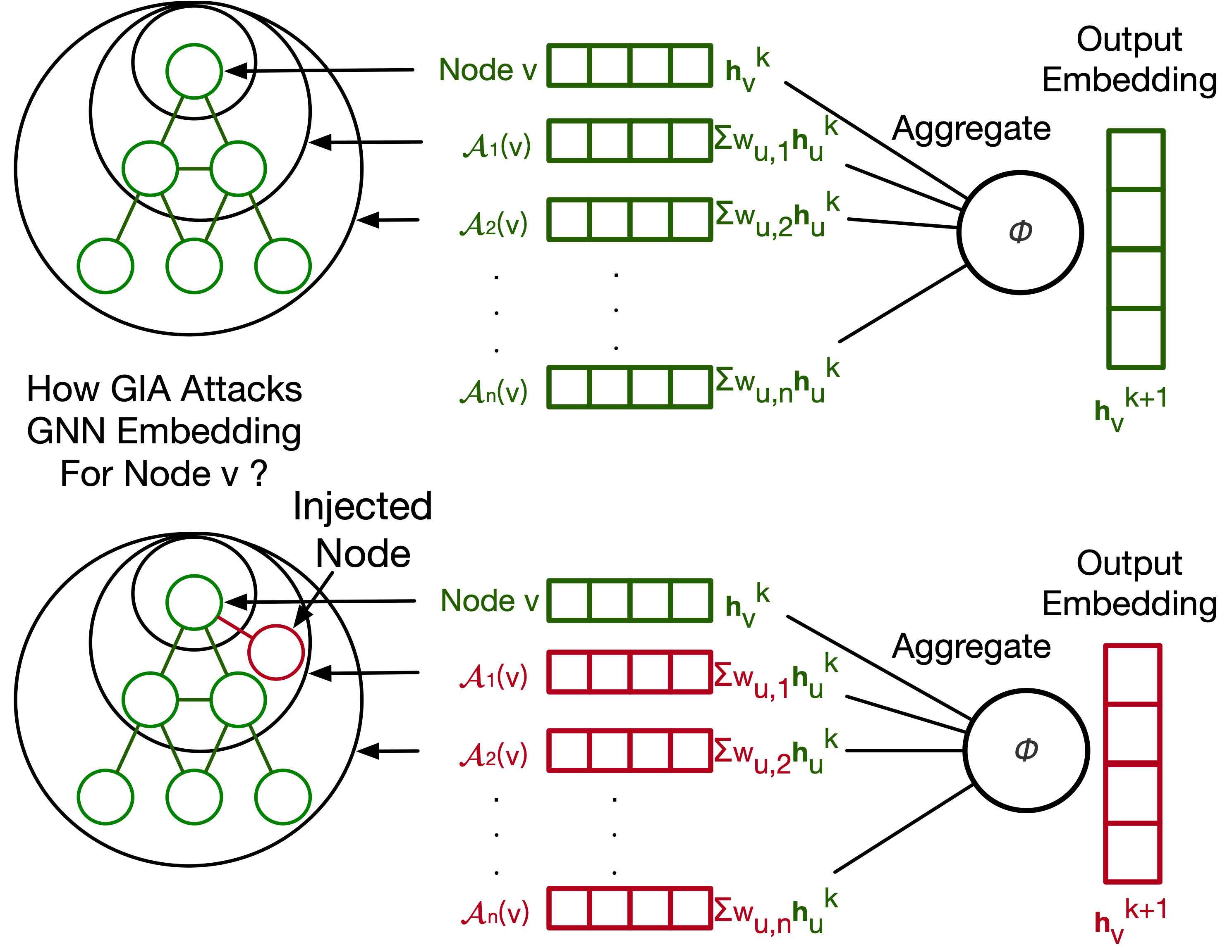
Figure 2. Top: A GNN layer aggregates information from $n$-hop neighbors of node $v$. Bottom: GIA perturbs the output embedding through $1$-hop node injection.

In order to better design injection attacks to GNNs, we explore the topological vulnerabilities of GNNs. Generally, a GNN layer performed on a node $v$ can be represented as the aggregation process (Hamilton et al., 2017; Xu et al., 2018):

(5) $$\mathbf{h}_{v}^{k}=\phi(\mathbf{h}_{v}^{k-1},\mathbf{f}(\{\mathbf{h}_{u}^{k-1}\}_{u\in\mathcal{A}(v)}))$$

where $\phi(\cdot)$ and $\mathbf{f}(\cdot)$ are vector-valued functions, $\mathcal{A}(v)$ denotes the neighborhood of node $v$, and $\mathbf{h}_{v}^{k}$ is the vector-formed hidden representation of node $v$ at layer $k$.

Note that $\mathcal{A}(v)$ include nodes that are directly connected to $v$ and nodes that can be connected to $v$ within certain number of steps. We use $\mathcal{A}_{t}(v)$ to represent the $t$-hop neighbors of $v$, i.e. nodes that can reach $v$ within $t$ steps. We use $\mathbf{f}_{t}(\cdot)$ as the corresponding aggregation functions. Therefore, Eq. 5 can be further expressed by

(6) $$\begin{split}\mathbf{h}_{v}^{k}=&\phi(\mathbf{f}_{0}(\mathbf{h}_{v}^{k-1}),\mathbf{f}_{1}(\{\mathbf{h}_{u}^{k-1}\}_{u\in\mathcal{A}_{1}(v)}),\mathbf{f}_{2}(\{\mathbf{h}_{u}^{k-1}\}_{u\in\mathcal{A}_{2}(v)}),\\ &...,\mathbf{f}_{n}(\{\mathbf{h}_{u}^{k-1}\}_{u\in\mathcal{A}_{n}(v)}))\end{split}$$

Suppose we perturb the graph by injecting nodes so that $\mathcal{A}_{t}$ changes to $\mathcal{A}^{\prime}_{t}$, and $\mathbf{f}_{t}$ is changed by a comparable small amount, i.e., $\mathbf{f}_{t}^{\prime}-\mathbf{f}_{t}=\Delta\mathbf{f}_{t}$. The new embedding for $v$ at layer $k$ becomes

(7) $$\begin{split}\mathbf{h}_{v}^{\prime k}=&\mathbf{h}_{v}^{k}+\frac{\partial\phi}{\partial\mathbf{f}_{0}}(\mathbf{f}_{0}^{\prime}-\mathbf{f}_{0})+\frac{\partial\phi}{\partial\mathbf{f}_{1}}(\mathbf{f}_{1}^{\prime}-\mathbf{f}_{1})+...+\frac{\partial\phi}{\partial\mathbf{f}_{n}}(\mathbf{f}_{n}^{\prime}-\mathbf{f}_{n})\\ &+O((\Delta\mathbf{f}_{0})^{2}+(\Delta\mathbf{f}_{1})^{2}+...+(\Delta\mathbf{f}_{n})^{2})\end{split}$$

By denoting $\frac{\partial\phi}{\partial\mathbf{f}_{t}}$ at layer $k$ as $\mathbf{p}_{t,k}$, we have

(8) $$\Delta\mathbf{h}_{v}^{k}=\mathbf{h}_{v}^{\prime k}-\mathbf{h}_{v}^{k}=\sum_{t=0}^{n}\mathbf{p}_{t,k}\Delta\mathbf{f}_{t}+o(\sum_{t}\Delta\mathbf{f}_{t})$$

Without loss of generality, we assume that $\mathbf{f}_{t}$ has the form of weighted average that is widely used in GNNs (Kipf and Welling, 2016; Wu et al., 2019; Zhu et al., 2019)

(9) $$\mathbf{f}_{t}(\{\mathbf{h}_{u}^{k-1}\}_{u\in\mathcal{A}_{t}(v)})=\sum_{u\in\mathcal{A}_{t}(v)}w_{u,t}\mathbf{h}_{u}^{k-1}$$

where the weight $w_{u,t}$ corresponds to the topological structure within $t$-hop neighborhood of node $v$. Therefore, we can exploit the topological vulnerabilities of GNNs under GIA setting by conducting $t$-hop node injection to construct $\mathcal{A}_{t}^{\prime}(v)$ and to perturb the output of $\mathbf{f}_{t}$

(10) $$\Delta\mathbf{f}_{t}=\sum_{u\in\mathcal{A}^{\prime}_{t}(v)}(\Delta w_{u,t}\mathbf{h}_{u}^{k-1}+w_{u,t}\Delta\mathbf{h}_{u}^{k-1})$$

Figure 2 represents an example of 1-hop node injection. The injected node can affect the embeddings of the $t$-hop neighborhoods of node $v$, resulting in final misclassification after the aggregation. The problem now becomes how to harness the topological vulnerabilities of the graph to conduct effective node injection.

5. The TDGIA Framework

We present the Topological Defective Graph Injection Attack (TDGIA) framework for effective attacks on graph neural networks. Its design is based on the vulnerability analysis of GNNs in Section 4. The overall process of TDGIA is illustrated in Figure 1 (b).

Specifically, TDGIA consists of two steps that corresponds to the general GIA process: topological defective edge selection and smooth adversarial optimization. First, we identify important nodes according to the topological properties of the original graph and inject new nodes around them sequentially. Second, to minimize the performance of node classification, we optimize the features of the injected nodes with a smooth loss function.

5.1. Topological Defective Edge Selection

In light of the topological vulnerability of a GNN layer (Cf. Section 4.2), we design an edge selection scheme to generate defective edges between injected nodes and original nodes to attack GNNs.

For a node $v$, TDGIA can change its $t$-hop neighbors $\mathcal{A}_{t}(v)$ to $\mathcal{A}^{\prime}_{t}(v)$. For original nodes $u\in\mathcal{A}_{t}(v)$, their features $\mathbf{h}_{u}$ remain unchanged. For injected nodes $u\in\mathcal{A}^{\prime}_{t}(v)\backslash\mathcal{A}_{t}(v)$, their features $\textbf{h}_{u}$ are initialized by zeros, then $\Delta\textbf{h}_{u}=\textbf{h}^{\prime}_{u}$. Then, Eq. 10 can be developed into

(11) $$\Delta\mathbf{f}_{t}=\sum_{u\in\mathcal{A}_{t}(v)}\Delta w_{u,t}{\mathbf{h}_{u}^{k-1}}+\sum_{u\in\mathcal{A}^{\prime}_{t}(v)\backslash\mathcal{A}_{t}(v)}w_{u,t}{\mathbf{h}_{u}^{\prime k-1}}$$

We start from attacking a single-layer GNN, i.e. $k=1$. According to Eq. 8, we shall maximize $\sum_{t=0}^{1}\mathbf{p}_{t1}\Delta\mathbf{f}_{t}$ to maximize $\Delta\mathbf{h}_{v}^{1}$. Note that $\Delta\mathbf{f}_{0}=\Delta\textbf{h}_{v}^{0}=\mathbf{0}$ since the original features are unchanged. Thus, we only need to maximize $\Delta\mathbf{f}_{1}$

(12) $$\Delta\mathbf{f}_{1}=\sum_{u\in\mathcal{A}_{1}(v)}\Delta w_{u,1}{\mathbf{h}_{u}^{0}}+\sum_{u\in\mathcal{A}^{\prime}_{1}(v)\backslash\mathcal{A}_{1}(v)}w_{u,1}{{\mathbf{h}}_{u}^{\prime 0}}$$

During edge selection stage, the features of injected nodes are not yet determined. Thus, our strategy is to first maximize the influence on $\sum w_{u,1},u\in\mathcal{A}^{\prime}_{t}(v)$ and to perturb $\Delta\mathbf{f}_{1}$ as much as possible.

We start from the common choices of $w_{u,1}$ used in GNNs. Following GCN (Kipf and Welling, 2016), various types of GNNs (Wu et al., 2019; Zhu et al., 2019; Du et al., 2017) use

(13) $$w_{u,1}=\frac{1}{\sqrt{deg(u)deg(v)}},u\in\mathcal{A}_{1}(v)$$

while mean-pooling based GNNs like GraphSAGE (Hamilton et al., 2017) use

(14) $$w_{u,1}=\frac{1}{deg(v)},u\in\mathcal{A}_{1}(v)$$

In TDGIA, when deciding which nodes the injected nodes should be linked to, we use a combination of weights from Eq. 13 and Eq. 14 to scale the topological vulnerability of node $v$:

(15) $$\lambda_{v}=k_{1}\frac{1}{\sqrt{deg(v)d}}+k_{2}\frac{1}{deg(v)}$$

where $deg(v)$ is the degree of the target node $v$ and $d$ is the budget on degree of injected nodes. The higher $\lambda_{v}$ is, the more likely a node may be attacked by GIA. In TDGIA, we connect injected nodes to existing nodes with higher $\lambda_{v}$ by constructing defective edges.

In Appendix A.2, we theoretically demonstrate that Eq. 10 can be generalized to multi-layer GNNs, thus this topological defective edge selection strategy still works under general GNNs.

5.2. Smooth Adversarial Optimization

Once the topological defective edges of injected nodes have been selected, the next step is to generate features for the injected nodes to advance the effect of the attacks. Specifically, given a model $\mathcal{M}$, an adjacency matrix $\mathbf{A}^{\prime}$ after node injection, we further optimize the features $\mathbf{F}_{I}$ of the injected nodes in order to (negatively) influence the model prediction $\mathcal{M}(\mathbf{A}^{\prime},\mathbf{F}^{{}^{\prime}})$. To that end, we design a smooth adversarial feature optimization with a smooth loss function.

Smooth Loss Function. Usually, in adversarial attack, we optimize reversely the loss function used for training a model. For example, we can use the inverse of KL divergence as the attack loss for a node $v$ in target set $\mathcal{T}$

(16) $$\mathcal{L}_{v}=-D_{KL}(\mathbf{Y}_{\text{pred}}||\mathbf{Y}_{\text{test}})=\ln(p_{y_{v,\text{pred}}=y_{v,\text{test}}})=\ln p_{v}$$

where $p_{v}$ is for simplicity the probability that $\mathcal{M}$ correctly classifies $v$. Using this loss may cause gradient explosion, as the derivative

(17) $$\frac{\partial\mathcal{L}_{v}}{\partial p_{v}}=\frac{\partial\ln p_{v}}{\partial p_{v}}=\frac{1}{p_{v}}$$

goes to $\infty$ when $p_{v}\rightarrow 0$. To prevent such unstable behavior during optimization, we use a smooth loss function

(18) $$\mathcal{L}_{v}=\max(r+\ln p_{v},0)^{2}$$

where $r$ is a control factor. Therefore the derivative becomes

(19) $$\frac{\partial\mathcal{L}_{v}}{\partial p_{v}}=\begin{cases}\frac{2(r+\ln p_{v})}{p_{v}},&e^{-r}<p_{v}\leq 1\\ 0,&0\leq p_{v}\leq e^{-r}\end{cases}$$

where $\frac{\partial\mathcal{L}_{v}}{\partial p_{v}}\rightarrow 0$ when $p_{v}\rightarrow 0$, and the optimization becomes stable. Finally, the objective is to find optimal features $F_{I}$ for injected nodes, which minimize the loss in Eq. 18 for all target nodes:

(20) $$\arg\min_{F_{I}}\frac{1}{|\mathcal{T}|}\sum_{v\in\mathcal{T}}\max(r+\ln p_{v},0)^{2}$$

Smooth Feature Optimization. Under GIA settings, there’s a constraint on the range of features of the injected nodes. Otherwise, the defenders can easily filter out injected nodes based on abnormal features. In TDGIA, we simply apply Clamp function during optimization process to limit the range of features

(21) $$Clamp(x,min,max)=\begin{cases}min,&x<min\\ x,&min<x<max\\ max,&x>max\end{cases}$$

However, this function may lead to zero gradient. If a feature exceeds the range, it will be stuck at maximal or minimal. To smooth the optimization process of TDGIA, we design a $Smoothmap$ function that remaps features onto $(min,max)$ smoothly by using

(22) $$Smoothmap(x,min,max)=\frac{max+min}{2}+\frac{max-min}{2}sin(x).$$

5.3. Overall attack process of TDGIA

In addition to topological defective edge selection and smooth adversarial optimization, we also include the sequential attack and the use of surrogate models in TDGIA.

Sequential Attack. In TDGIA, we adopt the idea of sequential attack (Wang et al., 2020) and inject nodes in batches. In each batch we add a small number of nodes to the graph, select their edges, and optimize their features. We repeat this process until the injection budget is fulfilled.

Surrogate Model. Under the black-box setting, the attacker has no information about the models being attacked, thus the attack has to be performed on a surrogate model. Specifically, we first train a surrogate model $\mathcal{M}$ using the given training data on the input graph and generate the surrogate labels $\{\hat{y}_{v},v\in\mathcal{T}\}$ using $\mathcal{M}$. Then we optimize the TDGIA attack to lower the accuracy of $\mathcal{M}$ for $\{\hat{y}_{v},v\in\mathcal{T}\}$. Note that when selecting defective edges, besides $\lambda_{v}$, we also use the correct probability $p_{v}$ based on the softmax output of $\mathcal{M}$ on node $v$ for its surrogate label $\hat{y}_{v}$. We then define the defective score $\mu_{v}$ as shown in Algorithm 1.

Complexity. Given a base model $\mathcal{M}$ with complexity $T$. Usually for GNNs $T=O(ED)$, where $E$ is the number of edges and $D$ being the dimension of input features. For edge selection, we needs to inference $\mathcal{M}$ once to generate $p_{v}$, which costs $O(T)$, and computation for $\lambda_{v}$ costs $O(E)=o(T)$, so the computation costs $O(T)$. For optimization, suppose $\Delta_{S}$ is the number of epochs and $B$ is the number of batches for sequential injection, the optimization costs $O(\Delta_{S}BT)$. So the overall complexity for TDGIA is $O(\Delta_{S}BT)$. In practice, $\Delta_{S}B$ for TDGIA is usually set to be smaller than the number of epochs for training $\mathcal{M}$, therefore generating attacks using TDGIA costs less time than training $\mathcal{M}$. TDGIA is very scalable and can work for any GNN as base model.

In summary, the attack of TDGIA is to first inject new nodes (and edges) into the original graph and then learn the features for the injected nodes. The injection of new nodes is determined by the topological vulnerabilities of the graph and GNNs. The features are learned via the smooth adversarial optimization. The overall attack process of TDGIA is illustrated in Algorithm 1.

Input: Original graph $\mathbf{G}=\{\mathbf{A},\mathbf{F}\}$; surrogate model $\mathcal{M}$;set of target nodes $\mathcal{T}$;

Output: Attacked graph $\mathbf{G}^{\prime}=(\mathbf{A}^{\prime},\mathbf{F}^{\prime})$;

Parameter : Budget on number of injected nodes $b$; budget on degree of each injected node $d$; constraint on range of features $\Delta_{F}$;

/* Initialization */

1 $\mathbf{G}^{\prime}\leftarrow\mathbf{G}$;$\mathbf{V}_{I}\leftarrow\mathbf{0}^{N\times N_{I}}$;$\mathbf{A}_{I}\leftarrow\mathbf{0}^{N_{I}\times N_{I}}$;$\mathbf{F}_{I}\leftarrow\mathcal{N}(0,\sigma)^{N_{I}\times D}$;

/* Sequential injection */

2 while $b>0$ do

       /* Topological Defective Edge Selection */

3       for $v\in\mathcal{T}$ do

4             Calculate the correct probability $p_{v}$ using $\mathcal{M}(\mathbf{G}^{\prime})$;

5             Calculate the defective factor $\lambda_{v}$ using Eq. 15;

6             Calculate the defective score $\mu_{v}=(\alpha p_{v}+(1-\alpha))\lambda_{v}$;

7            

8       end for

9      Set up the number of injected nodes $b_{\text{seq}}\leq b$;

10       $\mathbf{V}_{I}\leftarrow$ Connect $b_{\text{seq}}$ injected nodes to $b_{\text{seq}}\times d$ target nodes in $\mathcal{T}$ with the highest defective score $\mu_{v}$;

       /* Smooth Adversarial Optimization */

11       $\mathbf{F}_{I}\leftarrow$ Optimize the features of injected nodes smoothly (Eq. 20) using $Clamp$ (Eq. 21) and $Smoothmap$ (Eq. 22) ;

12       $b\leftarrow b-b_{\text{seq}}$, update the budget;

13       $\mathbf{A}^{\prime},\mathbf{F}^{\prime}\leftarrow$ Update $\mathbf{A}^{\prime}$ and $\mathbf{F}^{\prime}$ by $\mathbf{V}_{I}$, $\mathbf{F}_{I}$ using Eq. 2 and 3;

14       $\mathbf{G}^{\prime}\leftarrow(\mathbf{A}^{\prime},\mathbf{F}^{\prime})$;

15      

16 end while

return $\mathbf{G}^{\prime}$

Algorithm 1 The process of Topological Defective Graph Injection Attack (TDGIA).

6. Experiments

6.1. Basic Settings

Datasets. We conduct our experiments on three large-scale public datasets including 1) KDD-CUP dataset, a large-scale citation dataset used in KDD-CUP 2020 Graph Adversarial Attack & Defense competition 2) ogbn-arxiv (Hu et al., 2020), a benchmark citation dataset and 3) Reddit (Hamilton et al., 2017), a well-known online forum post dataset. Statistics of these datasets and injection constraints are displayed in Table 3.

Table 3. Statistics of datasets. We consider only unique undirected edges.

Dataset	Nodes	Train nodes	Val nodes	Test nodes	Edges	Features	Classes	Feature range	Injection feature range	Injected nodes	Injection degree limit
KDD-CUP	659,574	580,000	29,574	50,000	2,878,577	100	18	-1.74$\sim$1.63	-1$\sim$ 1	500	100
ogbn-arxiv	169,343	90,941	29,799	48,603	1,157,799	128	40	-1.39$\sim$1.64	-1$\sim$1	500	100
Reddit	232,965	153,932	23,699	55,334	11,606,919	602	41	-0.27$\sim$0.26	-0.25$\sim$0.25	500	100

Constraints. For each dataset, we set up the budget on the number of injected nodes $b=500$ and the budget on degree $d=100$. The feature limit $\Delta_{F}$ is set according to the range of features in the dataset (Cf Table 3). For experiments on KDD-CUP dataset, most submitted defense methods include preprocessing that filters out nodes with degree approaches to $100$. Therefore, in our experiments, we apply an artificial limit of 88 to avoid being filtered out. These constraints is applied to both TDGIA and baseline attack methods.

Evaluation Metric. To better evaluate GIA methods, we consider both the performance reduction and the transferability. Our evaluation is mainly based on the weighted average accuracy proposed in KDD-CUP dataset. The metric attaches a weight to each defense model based on its robustness under GIA, i.e. more robust defense gets higher weight. This encourages the adversary to focus on transferability across all defense models, and to design more general attacks. In addition to weighted average accuracy, we also provide the average accuracy among all defense models, and the average accuracy of the Top-3 defense models. The three evaluation metrics are formulated below:

(23) $$s_{\text{avg}}=\frac{1}{n}\sum_{i=1}^{n}s_{i},$$

(24) $$s_{\text{top-3}}=\frac{1}{n}\sum_{i=1}^{3}s_{i},$$

(25) $$\mathbf{f}_{t}=\sum_{u\in\mathcal{A}^{\prime}_{t}(v)}w_{v}\mathbf{h}_{u}^{k-1}$$

(26) $$s_{\text{weighted}}=\sum_{i=1}^{n}w_{i}s_{i},\sum_{i=1}^{n}w_{i}=1,w_{1}\geq w_{2}\geq...\geq w_{n}.$$

where $s_{1},s_{2},...s_{n}$ are descending accuracy scores of $n$ different defense models against one GIA attack, i.e. $s_{1}\geq s_{2}...\geq s_{n}$. For KDD-CUP dataset, we use the given weights, for ogbn-arxiv and Reddit, we set the weights in a similar way. More reproducibility details are introduced in Appendix A.1.

6.2. Attack & Defense Settings

Baseline Attack Methods. We compare our TDGIA approach with different baselines, including FGSM (Szegedy et al., 2013), AFGSM (Wang et al., 2020), and the SPEIT method (Zheng et al., 2020), the open-source attack method released by the champion team of KDD-CUP 2020. For KDD-CUP dataset we also include the top five attack submissions in addition to the above baselines. Specifically, FGSM and AFGSM are adapted to the GIA settings with black-box and evasion attacks. For FGSM (Szegedy et al., 2013), we randomly connect injected nodes to the target nodes, and optimize their features with inverse KL divergence (Eq. 16). AFGSM (Wang et al., 2020) offers an improvement to FGSM, we also adapt it to our GIA settings. Note that NIPA (Sun et al., 2020) covered in Table 1 is not scalable enough for the large-scale datasets.

Surrogate Attack Model. GCN (Kipf and Welling, 2016) is the most fundamental and most widely-used model among all GNN variants. Vanilla GCNs are easy to attack (Zügner et al., 2018; Wang et al., 2020). However, when incorporated with LayerNorm (Ba et al., 2016), it becomes much more robust. Therefore, it is used by some top-competitors in KDD-CUP and achieved good defense results. In our experiments, we mainly use GCN as the surrogate model to conduct transfer attacks. We use GCNs (with LayerNorm) with 3 hidden layers of dimension 256, 128, 64 respectively. Following the black-box setting, we first train the surrogate GCN model, perform TDGIA and various GIA on it, and transfer the injected nodes to all defense methods.

Baseline Defense Models. For KDD-CUP dataset, it offers 12 best defense submissions (including models and weights), which are considered as defense models. Note that these defense methods are well-formed, which are much more robust than weak methods like raw GCN (without LayerNorm or any other defense mechanism) evaluated in previous works (Zügner et al., 2018; Dai et al., 2018; Zügner and Günnemann, 2019; Wang et al., 2020; Sun et al., 2020). Most of top attack methods can lower the performance of raw GCN from $68.37\%$ to less than $35\%$. However, they can hardly reduce the $68.57\%$ weighted average accuracy on these defenses by more than $4\%$.

For Reddit and ogbn-arxiv datasets, we implement the 7 most representative defense GNN models (also appeared in top KDD-CUP defense submissions), GCN (Kipf and Welling, 2016) (with LayerNorm), SGCN (Wu et al., 2019), TAGCN (Du et al., 2017), GraphSAGE (Hamilton et al., 2017), RobustGCN (Zhu et al., 2019), GIN (Xu et al., 2018) and  (Klicpera et al., 2018) as defense models. We train these models on the original graph and fix them for defense evaluation against GIA methods. Details of these models are listed in Appendix A.1.

6.3. Performance of TDGIA

We use GCN(with LayerNorm) as our surrogate attack model for our experiments. We first evaluate the proposed TDGIA on KDD-CUP dataset. Table 4 illustrates the average performance of TDGIA and other GIA methods over 12 best defense submissions at KDD-CUP competition. Different from previous works, TDGIA aims at the common topological vulnerability of GNN layers, which makes it more transferable cross different defense GNN models. As can be seen, TDGIA significantly outperforms all baseline attack methods by a large margin with more than $8\%$ reduction on weighted average accuracy.

We also test the generalization ability of TDGIA on other datasets. As shown in Table 5, when attacking the 7 representative defense GNN models on Reddit and ogbn-arxiv, TDGIA still shows dominant performance on reducing the weighted average accuracy. This suggests that TDGIA can well generalize across different datasets.

To summarize, the experiments demonstrate that TDGIA is an effective injection attack method with promising transferability as well as generalization ability.

Table 4. Performance(%) of different GIA methods on KDD-CUP over 12 best KDD-CUP defense submissions.

	Attack Method	Average Accuracy	Top-3 Defense	Weighted Average	Reduction
Clean	-	65.54	70.02	68.57	-
KDD-CUP Top-5 Attack Submissions	advers	63.44	68.85	67.09	1.48
	dafts	63.91	68.50	67.02	1.55
	ntt	60.21	68.80	66.27	2.30
	simong	60.02	68.59	66.29	2.28
	u1234	61.18	67.95	64.87	3.70
Baseline Methods	FGSM	59.80	67.44	65.04	3.53
	AFGSM	59.22	67.37	64.74	3.83
	SPEIT	61.89	68.16	66.13	2.44
TDGIA	TDGIA	55.00	64.49	60.49	8.08

Table 5. Performance(%) of different GIA methods on Reddit and ogbn-arxiv over 7 representative defense models.

Dataset	Attack Method	Average Accuracy	Top-3 Defense	Weighted Average	Reduction
Reddit	Clean	94.86	95.94	95.62	-
	FGSM	92.26	94.61	93.80	1.82
	AFGSM	91.46	94.64	93.61	2.01
	SPEIT	93.35	94.27	93.99	1.63
	TDGIA	86.11	88.95	88.14	7.48
ogbn-arxiv	Clean	70.86	71.61	71.34	-
	FGSM	66.40	69.57	68.62	2.72
	AFGSM	62.60	69.08	66.96	4.38
	SPEIT	66.93	69.56	68.63	2.71
	TDGIA	57.00	59.23	58.53	12.81

6.4. Ablation Studies

In this section, we analyse in details the performance of TDGIA under different conditions, and TDGIA’s transferability when we use different surrogate models to attack different defense models.

Topological Defective Edge Selection. In Section 5.1 we propose a new edge selection method based on topological properties. We analysis the effect of this method by illustrating experimental results of different edge selection methods in Figure 3 (a). ”Uniform” method connects injected nodes to targeted nodes uniformly, i.e. each target node receives the same number of links from injected nodes, which is the most common strategy used by KDD-CUP candidates. ”Random” method randomly assigns links between target nodes and injected nodes. As illustrated, the topological defective edge selection contributes a lot to attack performance, and almost doubles the reduction on weighted accuracy of defense models.

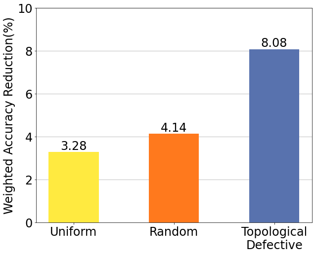
(a) Different Edge Selection Methods

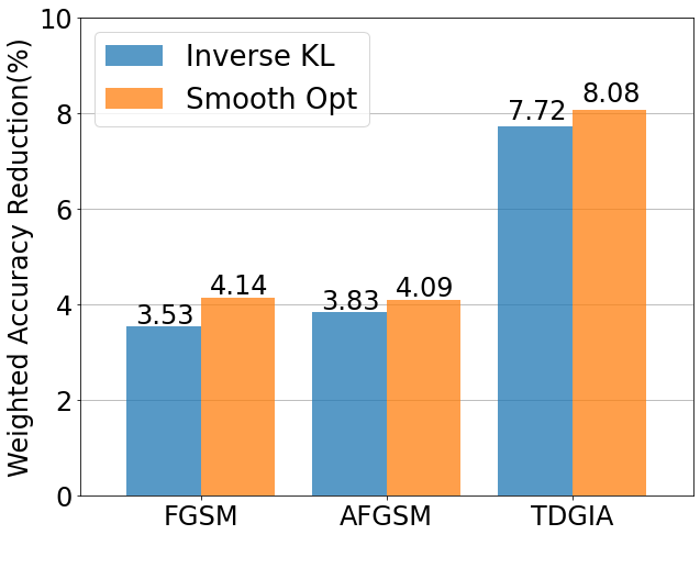
(b) Different Optimization Methods

Figure 3. Left:Performance of different edge selection methods based on smooth adversarial optimization. Right: Comparison of smooth adversarial optimization and inverse KL-divergence minimization. Results on KDD-CUP dataset.

Smooth Adversarial Optimization. The smooth adversarial optimization, proposed in Section 5.2, also has its own advantages. Figure 3 (b) shows the results of TDGIA and FGSM/AFGSM with/without smooth adversarial optimization. The strategy prevents the issues of gradient explosion and vanishing and does contribute to the attack performance of all three methods.

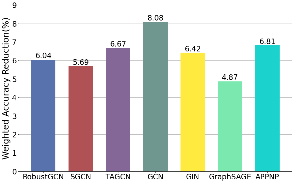
Figure 4. Weighted Accuracy Reduction of TDGIA on KDD-CUP dataset using different surrogate models for attack. GCN yields the best result.

Transferability across Different Models. We study the influence of different surrogate models on TDGIA. Figure 4 illustrates the transferability of TDGIA across different models. An interesting result is that GCN turns out to be the best surrogate model, i.e. TDGIA applied on GCN can be better transferred to other models.

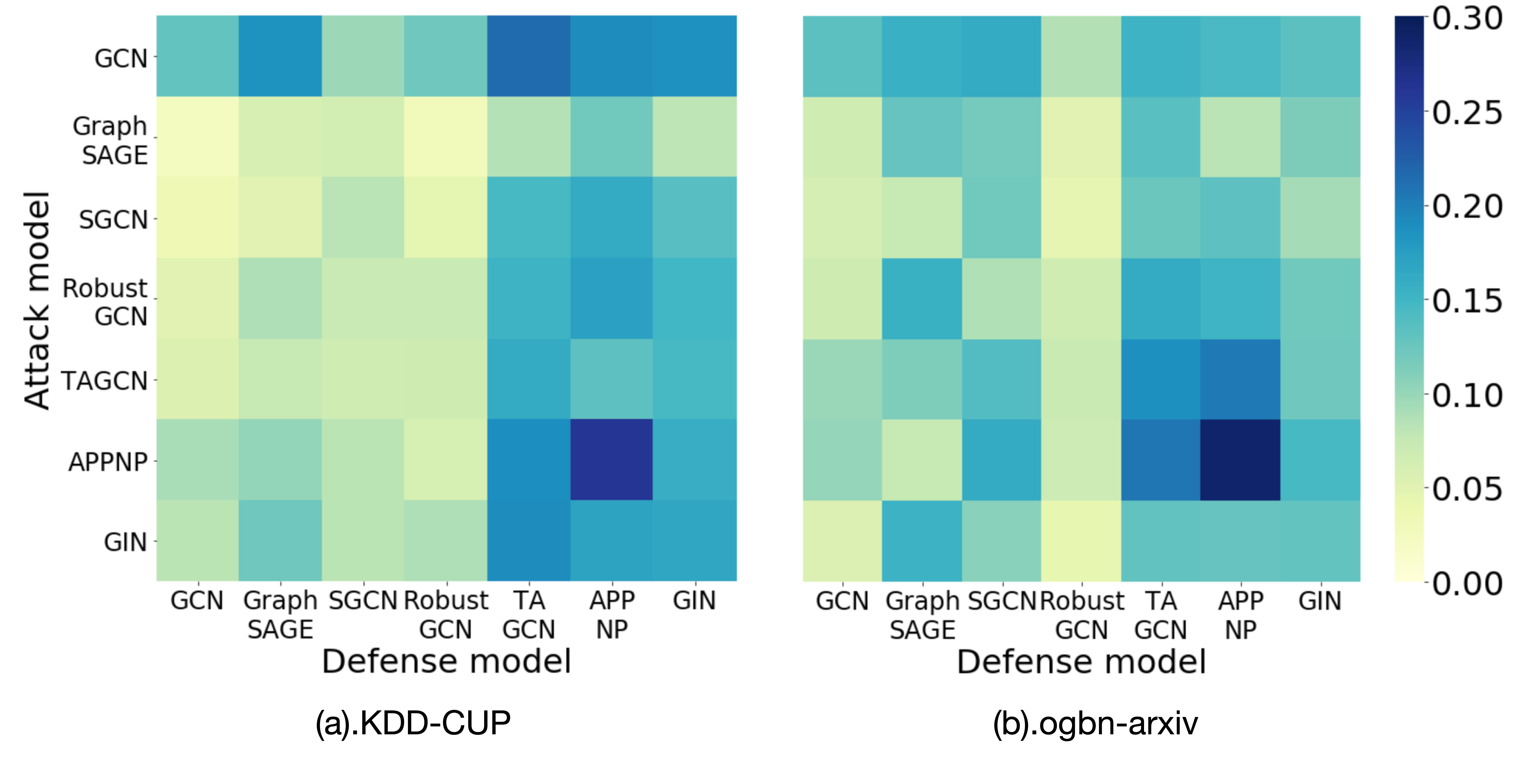
Figure 5. Transferability of TDGIA across different models. Using surrogate models for attack, and evaluate on defense models. Darker color suggests larger performance reduction. Left: KDD-CUP. Right: ogbn-arxiv.

Figure 5 further offers the visualization of transferability of TDGIA on KDD-CUP and ogbn-arxiv. The heat-map shows that TDGIA is effective for whatever surrogate model we use, and can be transferred to all defense GNN models listed in this paper, despite that the scale of transferability may vary. Again, we can see GCN yields attacks with better transferability. A probable explanation may be that most of GNN variants are designed based on GCN, making them more similar to GCN. Therefore, TDGIA can be better transferred using GCN as surrogate models. We also notice that RobustGCN is more robust as defense models, as it is intentionally designed to resist adversarial attacks. Still, our TDGIA is able to reduce its performance.

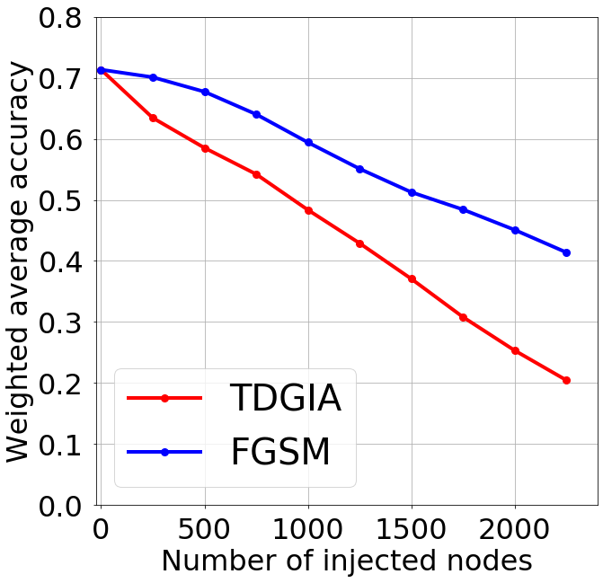
(a) TDGIA vs. FGSM (ogbn-arxiv)

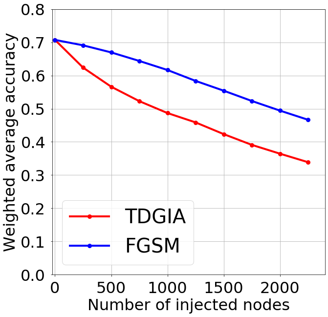
(b) TDGIA vs. FGSM (KDD-CUP)

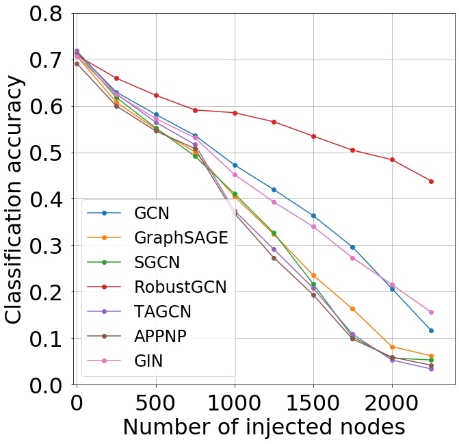
(c) TDGIA on Defense Models (ogbn-arxiv)

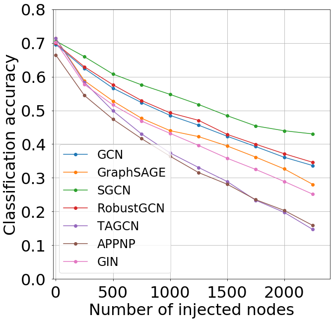
(d) TDGIA on Defense Models (KDD-CUP)

Figure 6. TDGIA under different numbers of injected nodes.

Magnitude of Injection. In previous experiments, we limit the number of injected nodes under 500. Note that this number is only $1\%$ compared to the number of target nodes. To show the power of TDGIA, we investigate the effect of the magnitude of injection. Figure 6 (a) (b) show the attack performance of TDGIA and FGSM on ogbn-arxiv and KDD-CUP datasets. For any magnitude of injection, TDGIA always outperforms FGSM significantly, with a gap for more than $10\%$ reduction on weighted average accuracy.

Figure 6 (c) (d) further illustrate the detailed performance of TDGIA on different defense models. When we expand the number of injected nodes, there is a continuous performance drop for all defense models. As the number increased to 2000, the accuracy of several defense models (e.g. GraphSAGE, SGCN, APPNP) even drop less than $10\%$. However, this number of injected nodes is still less than $5\%$ the size of target nodes, or $1.4\%$ (ogbn-arxiv) / $0.4\%$ (KDD-CUP) the size of the whole graph. The results demonstrate that most GNN models are quite vulnerable towards TDGIA.

7. Conclusion

In this work, we explore deeply into the graph injection attack (GIA) problem and present the TDGIA attack method. TDGIA consists of two modules: the topological defective edge selection for injecting nodes and smooth adversarial optimization for generating features of injected nodes. TDGIA achieves the best attack performance in attacking a variety of defense GNN models, compared with various baseline attack methods including the champion solution of KDD-CUP 2020. It is also worth mentioning that with only a few number of injected nodes, TDGIA is able to effectively attack GNNs under the black-box and evasion settings.

In this work, we mainly focus on leveraging the first level neighborhood on the graph to design the attack strategies. In the future, we would like to involve higher levels of neighborhood information for advanced attacks. Another interesting finding is that among all the GNN variants, using GCN as the surrogate model achieves the best results. Further studies on this observation may deepen our understandings of how different GNN variants work, and thus inspire more effective attack designs.

We continue our research on graph robustness issues and published Graph Robustness Benchmark on NeurIPS 2021. The work is called Graph Robustness Benchmark: Benchmarking the Adversarial Robustness of Graph Machine Learning(GRB) and we also created a website for attack and defense submissions, see GRB.

Appendix A Appendix

In appendix we follow the citation index in the main article.

A.1. Reproducibility Details

In this section, we introduce the experimental details for TDGIA.

Surrogate Attack Models. Under the black-box setting, we need to train surrogate models for attack. Each model is trained twice using different random seeds. The first one is the surrogate model. The second one is used as defense models. For KDD-CUP, we evaluate directly based on candidate submitted models and parameters. All models are trained for 10000 epochs using Adam, with a learning rate of 0.001 and dropout rate of 0.1. We evaluate the model on the validation set every 20 epochs and select the one with the highest validation accuracy to be the final model.

Detailed Description of Baseline Defense Models. In section 6.2, We only provide detailed introduction to GCN (with LayerNorm). Here we explain in detail about the other defense models.

SGCN (Wu et al., 2019). SGCN aims to simplify the GCN structure by removing the activations while improving the aggregation process. The method introduces more aggregation than other methods and thus has a much larger sensitivity area for each node, making the model more robust against tiny local neighborhood perturbations. We use an initial linear transformation that transforms the input into 140 dimensions, and 2 SGC layers with 120 and 100 channels respectively, with $k=4$ and LayerNorm, a final linear transformation that transfers that into the number of classes.

TAGCN (Du et al., 2017). TAGCN is a GCN variant that combines multiple-level neighborhoods in every single-layer of GCN. This is the method used by SPEIT, the champion of the competition. The model in our experiments has 3 hidden layers, each with 128 channels and with the propagation factor $k=3$.

GraphSAGE (Hamilton et al., 2017). GraphSAGE represents a type of node-based neighborhood aggregation mechanism, which aggregates direct neighbors on each layer. The aggregation function is free to adjust. Many teams use this framework in their submissions, their submissions vary in aggregation functions. We select a representative GraphSAGE method that aggregates neighborhoods based on $L_{2}$-norm of neighborhood features. The model has 4 hidden layers, each with 70 dimensions.

RobustGCN (Zhu et al., 2019). RobustGCN is a GCN variant designed to counter adversarial attacks on graphs. The model borrows the idea of random perturbation of features from VAE, and tries to encode both the mean and variation of the node representation and keep being robust against small perturbations. We use 3 hidden layers with 150 dimensions each.

GIN (Xu et al., 2018). GIN is introduced to maximize representation power of GNNs by aggregating self-connected features and neighborhood features of each node with different weights. Team ”Ntt Docomo Labs” uses this method as defensive model. We use 4 hidden layers with 144 dimensions each.

APPNP (Klicpera et al., 2018). APPNP is designed for fast approximation of personalized prediction for graph propagation. Like SGCN, APPNP propagates on graph dozens of times in a different way and therefore more robust to local perturbations. In application we first transform the input with a 2-layer fully-connected network with hidden size 128, then propagate for 10 times.

Attack Parameters. We conduct our attacks using batch-based smooth adversarial optimization. $r$ in Eq. 18 is set to 4. We follow the Algorithm 1. For $\lambda_{v}$ in Eq. 15, we take $k_{1}=0.9$ and $k_{2}=0.1$, for $\alpha$ mentioned in Algorithm 1 is set to 0.33. We don’t follow exactly the AFGSM description of one-by-one injection, as it costs too much time to optimize on large graphs with hundreds of injected nodes, instead we add nodes in batches, each batch contains nodes equal to $20\%$ of the injection budget, and is optimized under smooth adversarial optimization with Adam optimizer with a learning rate of $1$, features are initialized by $N(0,1)$. Each batch of injected nodes is optimized on surrogate models to lower its prediction accuracy on approximate test labels for 2,000 epochs.

Evaluation Mertric. The $w$ mentioned in Eq. 26 is set to $[0.24,0.18,0.12,0.1,0,08,0.07,0.06,0.05,0.04,0.03,0.02,0.01]$ in the KDD-CUP dataset, which offers a variety of 12 top candidate defense submissions. For evaluation on ogbn-arxiv and Reddit, $w$ is set to $[0.3,0,24,0.18,0.12,0.08,0.05,0.03]$ for the 7 defense models. In Figure 6 the KDD-CUP evaluation is based on the same models and weights as ogbn-arxiv.

Additional Information on Datasets. In the raw data of the Reddit dataset, unlike other dimensions, dimension 0 and 1 are integers ranging from 1 to 22737. We apply a transformation $f(x)=0.025\times\log(x)$ to regularize their range to $[-0.27,0.26]$ to match the scale of other dimensions. The ogbn-arxiv dataset has 1,166,243 raw links, however 8,444 of them are duplicated and only 1,157,799 are unique bidirectional links. So we take 1,157,799 as the number of links for ogbn-arxiv dataset.

A.2. Generalizing Topological Properties of Single-Layer GNN to Multi-Layer GNNs

In this section, we elaborate the topological properties of GNNs from single-layer to multi-layer. We show in multi-layer GNNs, the perturbation of $\mathbf{h}$ only relies on $\{\Delta w_{u,t}\|t=1,2...\}$, therefore the topological defective edge selection in Section 4.2 can be generalized to multi-layer GNNs.

We start from Eq. 10, for a GNN layer,

(27) $$\Delta\mathbf{f}_{t}=\sum_{u\in\mathcal{A}^{\prime}_{t}(v)}(\Delta w_{u,t}\mathbf{h}_{u}+w_{u,t}\Delta\mathbf{h}_{u})$$

Here, $\Delta w_{u}=w^{\prime}_{u}-w_{u},\Delta\mathbf{h}_{u}=\mathbf{h}^{\prime}_{u}-\mathbf{h}_{u}$ if $u\in\mathcal{A}^{\prime}_{t}(v)$ and $u\in\mathcal{A}_{t}(v)$. For $u\in\mathcal{A}^{\prime}_{t}(v),u\notin\mathcal{A}_{t}(v)$, $\Delta w_{u}=w^{\prime}_{u},\Delta\mathbf{h}_{u}=\mathbf{h}^{\prime}_{u}$. For GIA, $\mathcal{A}_{t}(v)\subseteq\mathcal{A}^{\prime}_{t}(v)$. Recall that $\mathbf{p}_{t,k}=\frac{\partial\mathbf{h}_{v}^{k}}{\partial\mathbf{f}_{t}}$. Then

(28) $$\Delta\mathbf{h}_{v}^{k}=\sum_{t=0}^{n}\mathbf{p}_{tk}\sum_{u\in\mathcal{A}^{\prime}_{t}(v)}(\Delta w_{u}\mathbf{h}_{u}^{k-1}+w_{u}\Delta\mathbf{h}_{u}^{k-1})$$

(29) $$\Delta\mathbf{h}_{v}^{k}=\sum_{t}\sum_{u\in\mathcal{A}^{\prime}_{t}(v)}(\Delta w_{u,t}\mathbf{p}_{t,k}\mathbf{h}_{u}^{k-1}+w_{u,t}\mathbf{p}_{tk}\Delta\mathbf{h}_{u}^{k-1})$$

This suggests that for single-layer GNNs the perturbation only relies on $\{\Delta w_{u,t}\|t=1,2...\}$.

Now let’s generalize this result to multi-layer GNNs using induction. Suppose $\Delta\mathbf{h}_{v}^{k}$ can be expressed in the following form

(30) $$\Delta\mathbf{h}_{v}^{k}=\sum_{t}\sum_{u\in\mathcal{A}^{\prime}_{t}(v)}(\Delta w_{u,t}\sum_{l=1}^{k}\mathbf{p}_{t,l}\mathbf{h}_{u}^{l-1}+w_{u,t}\mathbf{p}_{t,k}\Delta\mathbf{h}_{u}^{0})$$

For induction, suppose it holds for $k=n$,

(31) $$\begin{split}\Delta\mathbf{h}_{v}^{n+1}&=\sum_{t}\sum_{u\in\mathcal{A}^{\prime}_{t}(v)}(\Delta w_{u,t}\mathbf{p}_{t,k+1}\mathbf{h}_{u}^{k}+w_{u,t}\mathbf{p}_{t,k+1}\Delta\mathbf{h}_{u}^{k})\\ &=\sum_{t}\sum_{u\in\mathcal{A}^{\prime}_{t}(v)}(\Delta w_{u,t}\mathbf{p}_{t,k+1}\mathbf{h}_{u}^{k}+\\ &w_{u,t}\mathbf{p}_{t,k+1}\sum_{t^{\prime}}\sum_{u^{\prime}\in\mathcal{A}^{\prime}_{t^{\prime}}(u)}(\Delta w_{u^{\prime},t^{\prime}}\sum_{l=1}^{k-1}\mathbf{p}_{t^{\prime},l}\mathbf{h}_{u}^{l-1}+w_{u^{\prime},t^{\prime}}\mathbf{p}_{t^{\prime},k}\Delta\mathbf{h}_{u}^{0}))\\ &=\sum_{t}\sum_{u\in\mathcal{A}^{\prime}_{t}(v)}(\Delta w_{u,t}\sum_{l=1}^{k}\mathbf{p}^{\prime}_{t,l}\mathbf{h}_{u}^{l-1}+w_{u,t}\mathbf{p}^{\prime}_{t,k+1}\Delta\mathbf{h}_{u}^{0})\end{split}$$

where $\mathbf{p}^{\prime}$ is a function of the previous p. Therefore Eq. 30 holds for $k=n+1$. Also it obviously holds for $k=1$, by induction we conclude that Eq. 30 holds for all $k$. Therefore,

(32) $$\Delta\mathbf{h}_{v}^{n}=\sum_{t}\sum_{u\in\mathcal{A}^{\prime}_{t}(v)}(\Delta w_{u,t}\sum_{l=1}^{n}\mathbf{p}_{t,l}\mathbf{h}_{u}^{l-1}+w_{u,t}\mathbf{p}_{t,k}\Delta\mathbf{h}_{u}^{0})$$

And when we have $w_{u,t}=0,\forall u\notin\mathcal{G}$ for GIA, assuming $\Delta w_{u,t}<<1$, the function becomes

(33) $$\Delta\mathbf{h}_{v}^{n}=\sum_{t}\sum_{u\in\mathcal{A}^{\prime}_{t}(v)}\Delta w_{u,t}\sum_{l=1}^{n}\mathbf{p}_{t,l}\mathbf{h}_{u}^{l-1}$$

This means the perturbation on multi-layer GNNs also only relies on $\{\Delta w_{u,t}|t=1,2...\}$. Therefore, TDGIA can capture the topological weaknesses of them, which is also demonstrated what our extensive experiments on multi-layer GNNs.

A.3. Proof of Lemma 4.4

Proof.

Assume model $\mathcal{M}$ is non-structural-igonorant, then there exist $\mathbf{G}_{1}=(\mathbf{A}_{1},\mathbf{F}),\mathbf{G}_{2}=(\mathbf{A}_{2},\mathbf{F})$, $\mathbf{A}_{1}\neq\mathbf{A}_{2}$, $\mathcal{M}(\mathbf{G}_{1})\neq\mathcal{M}(\mathbf{G}_{2})$. Permute a common node of $\mathbf{G}_{1}$ and $\mathbf{G}_{2}$ to position 0, then

$$A_{1}=\left[\begin{array}[]{cc}0&B_{1}\\ C_{1}&S_{1}\\ \end{array}\right],A_{2}=\left[\begin{array}[]{cc}0&B_{2}\\ C_{2}&S_{2}\\ \end{array}\right]$$

$$B_{1},B_{2}\in\mathbb{R}^{1\times(N-1)},C_{1},C_{2}\in\mathbb{R}^{(N-1)\times 1},S_{1},S_{2}\in\mathbb{R}^{(N-1)\times(N-1)}$$

Consider a case of GIA in which nodes with the same features are injected to $\mathbf{G}_{1}$ and $\mathbf{G}_{2}$ in a different way, i.e. $\mathbf{G}_{1}^{*}=(\mathbf{A}_{1}^{*},\mathbf{F}^{*})$, $\mathbf{G}_{2}^{*}=(\mathbf{A}_{2}^{*},\mathbf{F}^{*})$ where

$$A_{1}^{*}=\left[\begin{array}[]{ccc}0&B_{1}&B_{2}\\ C_{1}&S_{1}&\textbf{0}\\ C_{2}&\textbf{0}&S_{2}\end{array}\right],A_{2}^{*}=\left[\begin{array}[]{ccc}0&B_{2}&B_{1}\\ C_{2}&S_{2}&\textbf{0}\\ C_{1}&\textbf{0}&S_{1}\end{array}\right]$$

Suppose $\mathcal{M}$ is not GIA-attackable, by Definition 4.2

(34) $$\mathcal{M}(\mathbf{G}_{1}^{*})=\mathcal{M}(\mathbf{G_{1}}),\mathcal{M}(\mathbf{G}_{2}^{*})=\mathcal{M}(\mathbf{G_{2}})$$

However, since $\mathcal{M}$ is permutation invariant, i.e. $\mathbf{G}_{1}^{*}$ and $\mathbf{G}_{2}^{*}$ are the same graph under permutation, then

(35) $$\mathcal{M}(\mathbf{G_{1}})=\mathcal{M}(\mathbf{G}_{1}^{*})=\mathcal{M}(\mathbf{G_{2}^{*}})=\mathcal{M}(\mathbf{G_{2}})$$

which contradicts to the initial assumption that $\mathcal{M}(\mathbf{G_{1}})\neq\mathcal{M}(\mathbf{G_{2}})$, so $\mathcal{M}$ is GIA-attackable. ∎

Table 6. Full Performance(%) table on KDD-CUP dataset including 28 competition submissions, baselines methods, and result of GIA using all 7 different surrogate attack models, evaluated on 12 top candidate submitted defenses in KDD-CUP 2020. Best results are bolded.

	Attack Method	Average Accuracy	Top-3 Defense	Weighted Average	Reduction
Clean	-	65.54	70.02	68.57	-
KDD-CUP Attacks	advers	63.44	68.85	67.09	1.48
	dafts	63.91	68.50	67.02	1.55
	deepb	61.44	69.4	67.26	1.31
	dminers	63.76	69.39	67.48	1.09
	fengari	63.78	69.41	67.45	1.12
	grapho	63.75	69.34	67.44	1.13
	msupsu	65.49	69.97	68.52	0.05
	ntt	60.21	68.80	66.27	2.30
	neutri	63.62	69.42	67.42	1.15
	runz	63.96	69.40	67.55	1.02
	speit	61.97	69.49	67.32	1.25
	selina	64.67	69.40	67.79	0.78
	tsail	63.90	69.40	67.55	1.02
	cccn	63.11	69.26	67.28	1.29
	dhorse	63.94	69.33	67.51	1.06
	kaige	63.90	69.41	67.49	1.08
	idvl	63.57	69.42	67.39	1.18
	hhhvjk	65.00	69.38	67.93	0.64
	fashui	63.69	69.42	67.42	1.15
	shengz	63.99	69.40	67.55	1.02
	sc	64.48	69.11	67.41	1.16
	simong	60.02	68.59	66.29	2.28
	tofu	63.87	69.39	67.50	1.07
	yama	64.21	68.77	67.23	1.34
	yaowen	63.94	69.33	67.50	1.07
	tzpppp	65.01	69.38	67.94	0.63
	u1234	61.18	67.95	64.87	3.70
	zhangs	63.73	69.43	67.51	1.06
Baseline Methods	FGSM	59.80	67.44	65.04	3.53
	FGSM (Smooth)	58.45	67.13	64.43	4.14
	AFGSM	59.22	67.37	64.74	3.83
	AFGSM (Smooth)	58.52	67.15	64.48	4.09
	SPEIT	61.89	68.16	66.13	2.44
TDGIA with different surrogate models	RobustGCN	57.24	65.83	62.53	6.04
	sgcn	58.01	66.28	62.88	5.69
	tagcn	58.35	65.82	62.90	5.67
	GCN	55.00	64.49	60.49	8.08
	GIN	56.83	65.70	62.15	6.42
	GraphSAGE	59.35	66.43	63.70	4.87
	appnp	55.80	65.93	61.76	6.81

References

- (1)
- Athalye et al. (2018) Anish Athalye, Nicholas Carlini, and David Wagner. 2018. Obfuscated gradients give a false sense of security: Circumventing defenses to adversarial examples. In ICML’18. PMLR, 274–283.
- Ba et al. (2016) Jimmy Lei Ba, Jamie Ryan Kiros, and Geoffrey E Hinton. 2016. Layer normalization. arXiv preprint arXiv:1607.06450 (2016).
- Carlini and Wagner (2017) Nicholas Carlini and David Wagner. 2017. Towards evaluating the robustness of neural networks. In 2017 IEEE Symposium on Security and Privacy. IEEE, 39–57.
- Carlini and Wagner (2018) Nicholas Carlini and David Wagner. 2018. Audio adversarial examples: Targeted attacks on speech-to-text. In 2018 IEEE Security and Privacy Workshops. IEEE.
- Dai et al. (2018) Hanjun Dai, Hui Li, Tian Tian, Xin Huang, Lin Wang, Jun Zhu, and Le Song. 2018. Adversarial Attack on Graph Structured Data. In ICML’18.
- Du et al. (2017) Jian Du, Shanghang Zhang, Guanhang Wu, José MF Moura, and Soummya Kar. 2017. Topology adaptive graph convolutional networks. arXiv preprint arXiv:1710.10370 (2017).
- Goodfellow et al. (2014a) Ian Goodfellow, Jean Pouget-Abadie, Mehdi Mirza, Bing Xu, David Warde-Farley, Sherjil Ozair, Aaron Courville, and Yoshua Bengio. 2014a. Generative adversarial nets. In NeurIPS’14. 2672–2680.
- Goodfellow et al. (2014b) Ian J Goodfellow, Jonathon Shlens, and Christian Szegedy. 2014b. Explaining and harnessing adversarial examples. arXiv preprint arXiv:1412.6572 (2014).
- Hamilton et al. (2017) Will Hamilton, Zhitao Ying, and Jure Leskovec. 2017. Inductive representation learning on large graphs. In NeurIPS’17. 1024–1034.
- Hu et al. (2020) Weihua Hu, Matthias Fey, Marinka Zitnik, Yuxiao Dong, Hongyu Ren, Bowen Liu, Michele Catasta, and Jure Leskovec. 2020. Open graph benchmark: Datasets for machine learning on graphs. arXiv preprint arXiv:2005.00687 (2020).
- Huang et al. (2017) Sandy Huang, Nicolas Papernot, Ian Goodfellow, Yan Duan, and Pieter Abbeel. 2017. Adversarial attacks on neural network policies. arXiv preprint arXiv:1702.02284 (2017).
- Jiang et al. (2020) Mingjian Jiang, Zhen Li, Shugang Zhang, Shuang Wang, Xiaofeng Wang, Qing Yuan, and Zhiqiang Wei. 2020. Drug–target affinity prediction using graph neural network and contact maps. RSC Advances 10, 35 (2020), 20701–20712.
- Jin et al. (2021) Wei Jin, Yaxing Li, Han Xu, Yiqi Wang, Shuiwang Ji, Charu Aggarwal, and Jiliang Tang. 2021. Adversarial Attacks and Defenses on Graphs. ACM SIGKDD Explorations Newsletter 22, 2 (2021), 19–34.
- Kipf and Welling (2016) Thomas N Kipf and Max Welling. 2016. Semi-supervised classification with graph convolutional networks. arXiv preprint arXiv:1609.02907 (2016).
- Klicpera et al. (2018) Johannes Klicpera, Aleksandar Bojchevski, and Stephan Günnemann. 2018. Predict then propagate: Graph neural networks meet personalized pagerank. arXiv preprint arXiv:1810.05997 (2018).
- Li et al. (2019) J Li, S Ji, T Du, B Li, and T Wang. 2019. TextBugger: Generating Adversarial Text Against Real-world Applications. In 26th Annual Network and Distributed System Security Symposium.
- Sun et al. (2020) Yiwei Sun, Suhang Wang, Xianfeng Tang, Tsung-Yu Hsieh, and Vasant Honavar. 2020. Adversarial Attacks on Graph Neural Networks via Node Injections: A Hierarchical Reinforcement Learning Approach. In WWW’20. 673–683.
- Szegedy et al. (2013) Christian Szegedy, Wojciech Zaremba, Ilya Sutskever, Joan Bruna, Dumitru Erhan, Ian Goodfellow, and Rob Fergus. 2013. Intriguing properties of neural networks. arXiv preprint arXiv:1312.6199 (2013).
- Wang et al. (2020) Jihong Wang, Minnan Luo, Fnu Suya, Jundong Li, Zijiang Yang, and Qinghua Zheng. 2020. Scalable Attack on Graph Data by Injecting Vicious Nodes. arXiv preprint arXiv:2004.13825 (2020).
- Wu et al. (2019) Felix Wu, Amauri Souza, Tianyi Zhang, Christopher Fifty, Tao Yu, and Kilian Weinberger. 2019. Simplifying graph convolutional networks. In ICML’19. PMLR, 6861–6871.
- Xu et al. (2018) Keyulu Xu, Weihua Hu, Jure Leskovec, and Stefanie Jegelka. 2018. How Powerful are Graph Neural Networks?. In ICLR’18.
- Ying et al. (2018) Rex Ying, Ruining He, Kaifeng Chen, Pong Eksombatchai, William L Hamilton, and Jure Leskovec. 2018. Graph convolutional neural networks for web-scale recommender systems. In KDD’18. 974–983.
- Zheng et al. (2020) Qinkai Zheng, Yixiao Fei, Yanhao Li, Qingmin Liu, Minhao Hu, and Qibo Sun. 2020. KDD CUP 2020 ML Track 2 Adversarial Attacks and Defense on Academic Graph 1st Place Solution. https://github.com/Stanislas0/KDD_CUP_2020_MLTrack2_SPEIT.
- Zhu et al. (2019) Dingyuan Zhu, Ziwei Zhang, Peng Cui, and Wenwu Zhu. 2019. Robust graph convolutional networks against adversarial attacks. In KDD’19. 1399–1407.
- Zügner et al. (2018) Daniel Zügner, Amir Akbarnejad, and Stephan Günnemann. 2018. Adversarial attacks on neural networks for graph data. In KDD’18. 2847–2856.
- Zügner and Günnemann (2019) Daniel Zügner and Stephan Günnemann. 2019. Adversarial attacks on graph neural networks via meta learning. arXiv preprint arXiv:1902.08412 (2019).