Equivariant Networks for Pixelized Spheres

Abstract

Pixelizations of Platonic solids such as the cube and icosahedron have been widely used to represent spherical data, from climate records to Cosmic Microwave Background maps. Platonic solids have well-known global symmetries. Once we pixelize each face of the solid, each face also possesses its own local symmetries in the form of Euclidean isometries. One way to combine these symmetries is through a hierarchy. However, this approach does not adequately model the interplay between the two levels of symmetry transformations. We show how to model this interplay using ideas from group theory, identify the equivariant linear maps, and introduce equivariant padding that respects these symmetries. Deep networks that use these maps as their building blocks generalize gauge equivariant CNNs on pixelized spheres. These deep networks achieve state-of-the-art results on semantic segmentation for climate data and omnidirectional image processing. Code is available at https://git.io/JGiZA.

1 Introduction

Representing signals on the sphere is an important problem across many domains; in geodesy and astronomy, discrete maps assign scalars or vectors to each point on the surface of the earth or points in the sky. To this end, various pixelizations or tilings of the sphere, often based on Platonic solids, have been used. Here, each face of the solid is refined using a triangular, hexagonal, or square grid and further recursive refinements can bring the resulting polyhedron closer and closer to a sphere, enabling an accurate projection from the surface of a sphere; see Fig. 2.

Our objective is to enable deep learning on this representation of spherical signals. A useful learning bias when dealing with structured data is to design equivariant models that preserve the symmetries of the structure at hand; the equivariance constraint ensures that symmetry transformations of the data result in the same symmetry transformations of the representation. To this end, we first need to identify the symmetries of pixelized spheres.

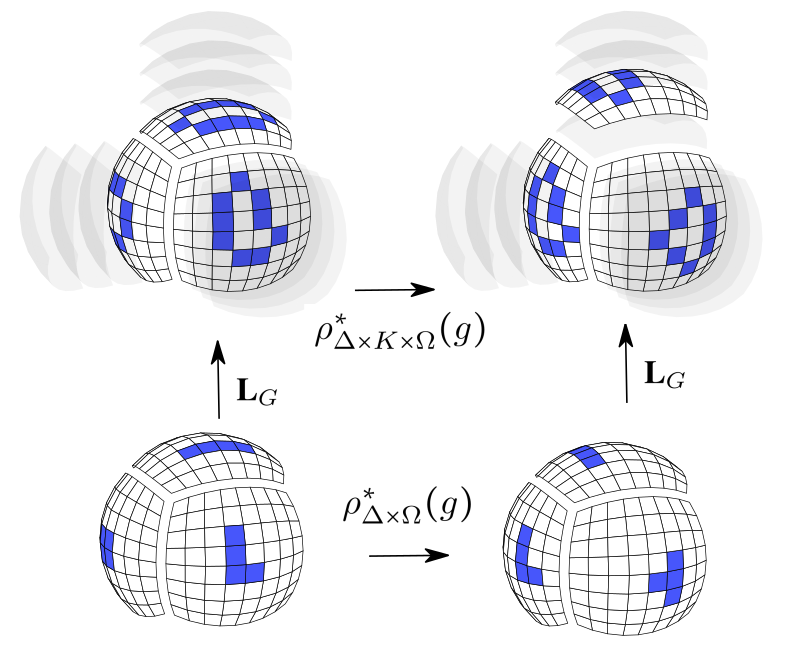
Figure 1: We model the rotational symmetry of the sphere by combining the rotational symmetry of a Platonic solid and isometries of each of its face grids. The bottom row shows one such symmetry transformation for scalar features on the quad sphere. The top row shows the corresponding transformation for regular features. Note that the $90^{\circ}$ rotation of the cube around the vertical axis also rolls the feature grids on top, in addition to rotating them. We identify the equivariant linear maps that make this diagram commute.

While Platonic solids have well-known symmetries (Coxeter, 1973), their pixelization does not simply extend these symmetries. To appreciate this point it is useful to contrast the situation with the pixelization of a circle using a polygon: when using an $m$-gon, the cyclic group ${C}_{m}$ approximates the rotational symmetry of the circle, ${SO}(2)$. By further pixelizing and projecting each edge of the $m$-gon using $2$ pixels, we get a regular $2m$-gon, with a larger symmetry group ${C}_{m}<{C}_{2m}<{SO}(2)$ – therefore in this case further pixelization simply extends the symmetry. However, this does not happen with the sphere and its symmetry group ${SO}(3)$ – that is, pixelized spheres are not homogeneous spaces for any finite subgroup of ${SO}(3)$.

One solution to this problem proposed by Cohen et al. (2019a) is to design deep models that are equivariant to “local” symmetries of a pixelized sphere. However, the symmetry of the solid is ignored in gauge equivariant CNNs. In fact, we show that under some assumptions, the gauge equivariant model can be derived by assuming a two-level hierarchy of symmetries (Wang et al., 2020), where the top-level symmetry is the complete exchangeability of faces (or local charts). A natural improvement is to use the symmetry of the solid to dictate valid permutations of faces instead of assuming complete exchangeability.

While the previous step is an improvement in modeling the symmetry of pixelized spheres, we observe that a hierarchy is inadequate because it allows for rotation/reflection of each face tiling independent of rotations/reflections of the solid. This choice of symmetry is too relaxed because the rotations/reflections of the solid completely dictate the rotation/reflection of each face-tiling. Using the idea of block systems from permutation group theory, we are able to enforce inter-relations across different levels of the hierarchy, composed of the solid and face tilings. After identifying this symmetry transformation, we identify the family of equivariant maps for different choices of Platonic solid. We also introduce an equivariant padding procedure to further improve the feed-forward layer.

The equivariant linear maps are used as a building block in equivariant networks for pixelized spheres. Our empirical study using different pixelizations of the sphere demonstrates the effectiveness of our choice of approximation for spherical symmetry, where we report state-of-the-art on popular benchmarks for omnidirectional semantic segmentation and segmentation of extreme climate events.

2 Pixelizing the Sphere

To pixelize the sphere one could pixelize the faces of any polyhedron with transitive faces – that is, any face is mapped to any other face using a symmetry transformation (Popko, 2012). Such a polyhedron is called an isohedron. For example, the Quadrilateralized Spherical Cube (quad sphere) pixelizes the sphere by defining a square grid on a cube. This pixelization was used in representing sky maps by the COsmic Background Explorer (COBE) satellite. Alternatively, pixelization of the icosahedron using hexagonal grids for similar applications in cosmology is studied in Tegmark (1996). Today, a pixelization widely used to map the sky is Hierarchical Equal Area isoLatitude Pixelization (HEALPix), which pixelizes the faces of a rhombic dodecahedron, an isohedron that is not a Platonic solid.

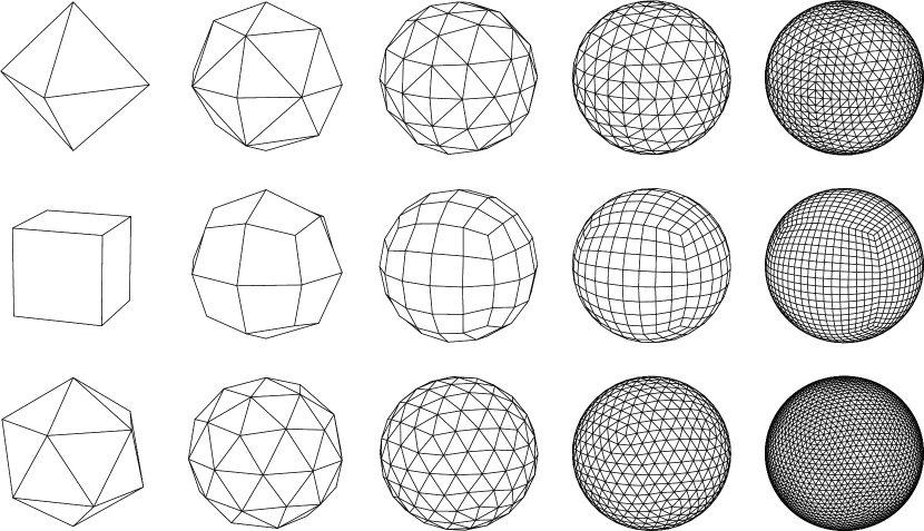
Figure 2: Iterative pixelization and projection for three Platonic solids: in each iteration (left-to-right), the pixels are recursively subdivided and projected onto the circumscribed sphere.

Platonic solids are more desirable as a model of the sphere because they are the only convex isohedra that are face-edge-vertex transitive – that is, not only can we move any face to another face using symmetry transformations, but we can also do this for edges and vertices. Similarly, there are only three regular tilings of the plane with this property: triangular, hexagonal, and square grids. Platonic solids give a regular tiling of the sphere, and this tiling is further refined by recursive subdivision and projection of each tile onto the sphere; see Fig. 2. A large family of geodesic polyhedra use a triangular tiling to pixelize some Platonic solids, including the tetrahedron, octahedron, and icosahedron. In our treatment, we assume that rotation/reflection symmetries of each face match the rotation/reflection symmetries of the tiling – e.g., square tiling is only used with a cube because both the square face of the cube and square grid have $90^{\circ}$ rotational symmetries. We exclude the dodecahedron because its triangular face tiling does not have translational symmetry.

3 Preliminaries

Let $[v]=\{1,\ldots,v\}$ denote the vertex set of a given Platonic solid. Each face $f\in[v]^{m}$ of the solid is an $m$-gon identified by its $m$ vertices, and $\Delta\subset[v]^{m}$ is the set of all faces. The action of the solid’s symmetry group ${H}$, a.k.a. polyhedral group, on faces $\Delta$ defines the permutation representation $\pi:{H}\to{Sym}(\Delta)$ that maps each group member to a permutation of faces. Here ${Sym}(\Delta)$ is the group of all permutations of $\Delta$. We use $\pi({H})$ to make this dependence explicit. Sometimes a subscript is used to identify the ${H}$-set – for example, $\pi_{\Delta}({H})$ and $\pi_{[v]}({H})$ define ${H}$ action on faces and vertices of the solid respectively. Since as a permutation matrix $\bm{\pi}({h}):\mathds{R}^{|\Delta|}\to\mathds{R}^{|\Delta|}$ for ${h}\in{H}$ is also a linear map, we use a bold symbol in this case to make the distinction. For the same reason, we use $\Delta$ and $\mathds{R}^{|\Delta|}$ interchangeably for the corresponding ${H}$-set.

3.1 Symmetries of the Face Tiling

Here, we focus on the symmetries of a single tiled face. Each face has a regular tiling using a set $\Omega$ of tiles or pixels. This regular tiling has its own symmetries, composed of 2D translations $\tau({T})<{Sym}(\Omega)$, and rotations/reflections $\kappa({K})<{Sym}(\Omega)$. When we consider rotational or chiral symmetries ${K}={C}_{m}$ is the cyclic group, and when adding reflections, we have ${K}={D}_{m}$, the dihedral group.

When combining translations and rotations/reflections one could simply perform translation followed by rotation/reflection. However, since a similar form of a combination of two transformations appears later in the paper (when we combine the rotations of the solid with translations on all faces), in the following paragraph, we take a more formal route to explain why the combination of rotation/reflection and translation takes this simple form.

The rotation/reflection symmetries of the tiling define an automorphism of translations $a:{K}\to{Aut}({T})$ – e.g., horizontal translation becomes vertical translation after a $90^{\circ}$ rotation. This automorphism defines the semi-direct product ${U}={K}\rtimes_{a}{T}$ as the abstract symmetry of the tiling. The action of members of this new group $({k},{t})={u}\in{U}$, on the tiles $\Omega$ is a permutation group $\upsilon({U})<{Sym}(\Omega)$

$$\bm{\upsilon}_{\Omega}({u})=\underbrace{\left(\bm{\kappa}({k})\bm{\tau}({t}){\bm{\kappa}({k}^{-1})}\right)}_{\text{automorphism}\;a_{k}({t})}\bm{\kappa}{({k})}=\bm{\kappa}{({k})}\bm{\tau}{({t})}.$$ (1)

In the group action above, the automorphism of translations is through conjugation by ${K}$, where ${K}$ itself also rotates/reflects the input. The end result becomes translation followed by rotation/reflection, as promised.

The action above permutes individual pixels and therefore assumes scalar features attached to each pixel. An alternative is to define vector features so that ${U}$ action becomes regular. For this we attach a vector of length $|{K}|$ to each pixel, and use the regular ${K}$ action on itself $\bm{\kappa}_{K}:{K}\to{Sym}({K})$ to define ${U}$ action on the Cartesian product ${K}\times\Omega$

$$\bm{\upsilon}_{{K}\times\Omega}{({k},{t})}=\bm{\kappa}_{K}{({k})}\otimes\left(\bm{\kappa}_{\Omega}{({k})}\bm{\tau}{({t})}\right),$$ (2)

where $\otimes$ is the tensor product. In words, ${U}$ action on ${K}\times\Omega$ translates and rotates/reflects the pixels $\Omega$ and at the same time transforms the vectors or fibers ${K}$.

Example 1 (Quad Sphere).

Full symmetries of the cube is a subgroup of the orthogonal group ${H}<{O}(3)$. The corresponding rotations/reflections are represented by $3\times 3$ rotation/reflection matrices that have $\pm 1$ entries with only one non-zero per row and column. There are $2^{3}$ choices for the sign and $3!=6$ choices for the location of these non-zeros, creating a group of size $6\times 8=48$. Half of these matrices have a determinant of one and therefore correspond to rotational symmetries. For simplicity, in the follow-up examples, we consider only these symmetries. The resulting group is isomorphic to the symmetric group ${S}_{4}$, where each rotation corresponds to some permutation of the four long diagonals of the cube. Now consider a $d\times d$ square tiling of each face of the cube, i.e., $|\Omega(f)|=d^{2}$. In addition to translational symmetry ${T}={C}_{d}\times{C}_{d}$, the cyclic group ${K}={C}_{4}$ represents the rotational symmetry of the grid. ${U}$ action simply performs translation followed by rotation in multiples of $90^{\circ}$.

3.2 Equivariant Linear Maps for Each Face

Given the permutation representations $\upsilon_{{K}\times\Omega}({U})$, a linear map $\textbf{{{L}}}:\mathds{R}^{|{K}\times\Omega|}\to\mathds{R}^{|{K}\times\Omega|}$ is ${U}$-equivariant if $\textbf{{{L}}}\bm{\upsilon}({u})=\bm{\upsilon}({u})\textbf{{{L}}}$ for all ${u}\in{U}$, or in other words

$$\textbf{{{L}}}=\bm{\upsilon}({u})\textbf{{{L}}}\bm{\upsilon}({u})^{\top}\quad\forall{u}\in{U}.$$

Using a tensor product property we can rewrite this constraint as

$$\operatorname{vec}(\textbf{{{L}}})=\bm{\upsilon}^{2}({u})\operatorname{vec}(\textbf{{{L}}})\quad\forall{u}\in{U},$$

where $\bm{\upsilon}^{2}({u})\doteq\bm{\upsilon}({u})\otimes\bm{\upsilon}({u})$ is a permutation action of ${u}\in{U}$ on $\mathbb{A}={K}\times\Omega\times{K}\times\Omega$, the elements of the “weight matrix” L. The orthogonal bases for which this condition holds are $|{K}\times\Omega|\times|{K}\times\Omega|$ binary matrices $\textbf{{{L}}}_{(1)},\ldots,\textbf{{{L}}}_{(\ell)}$ that are simply identified by the orbits of $\upsilon^{2}({U})$ action on $\mathbb{A}$ (Wood & Shawe-Taylor, 1996; Ravanbakhsh et al., 2017). The question of finding the linear bases is therefore the same as that of finding the orbits of permutation groups. We can use orbit finding algorithms from group theory with time complexity that is linear in the number of input-outputs (i.e., size of the matrix, or cardinality of $\mathbb{A}$), and the size of the generating set of the group, ${G}^{*}\subseteq{G}$ s.t. $\langle{G}^{*}\rangle={G}$ (Hiß et al., 2007). Algorithm 1 in the Appendix gives the pseudo-code for finding the orbit of a given element $a\in\mathbb{A}$. The fact that orthogonal bases are binary means that ${U}$-equivariant linear maps are parameter-sharing matrices, where each basis identifies a set of tied parameters and its nonzero elements correspond to an orbit of ${U}$ action on $\mathbb{A}$. We have implemented this procedure for automated creation of parameter-sharing matrices and made the code available.

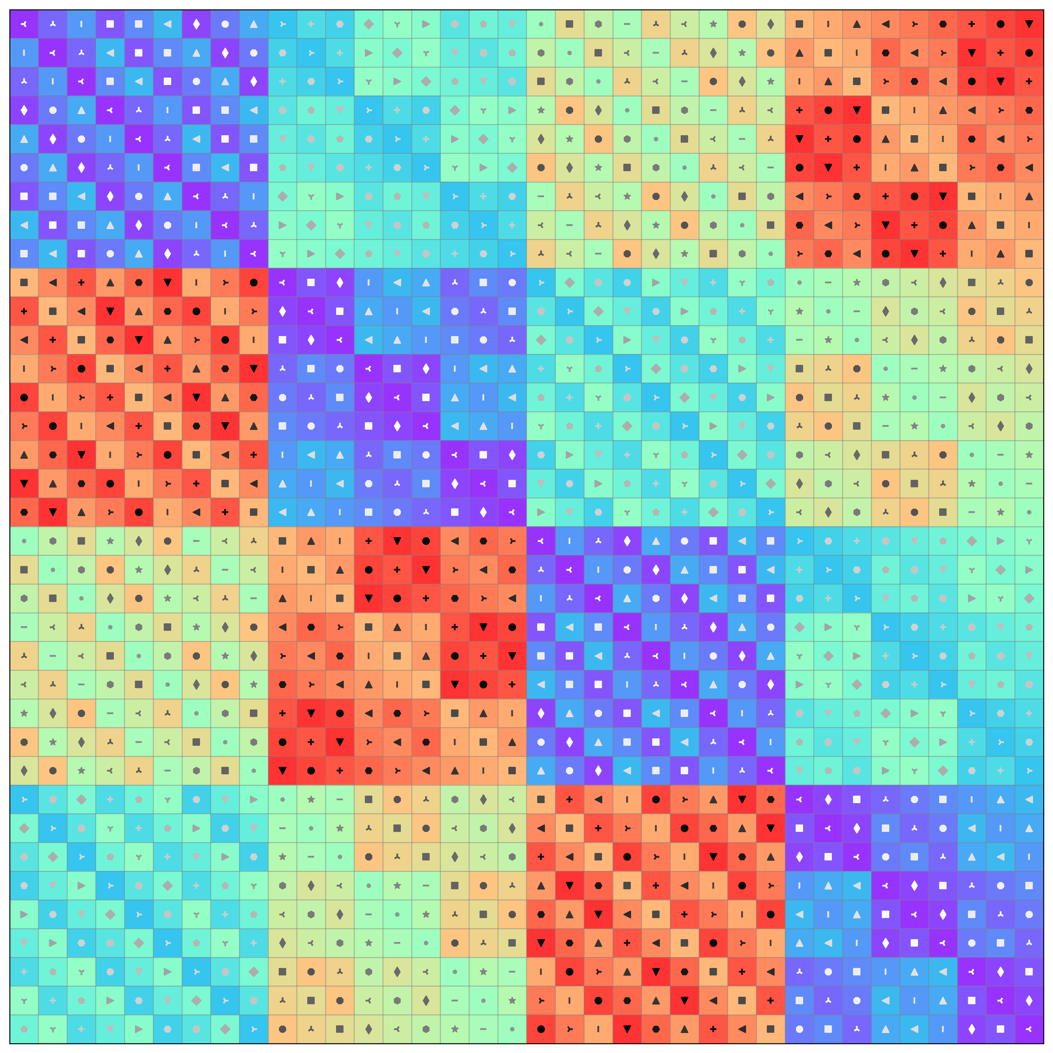
Figure 3: The parameter-sharing matrix for $\textbf{{{L}}}_{U}$. This linear map is equivariant to circular translations and $90^{\circ}$ rotations of regular feature vectors on a $3\times 3$ grid. That is, ${K}={C}_{4}$ and $|\Omega|=3\times 3=9$. Note that this matrix is the parameter-sharing equivalent of having ${C}_{4}$-steerable filters.

To increase the expressivity of the deep network that deploys this kind of linear map, we may have multiple input and output channels, and for each input-output channel pair, we use a new set of parameters. An alternative characterization of equivariant linear maps is through group convolution, where the semi-direct product construction of ${U}$ leads to ${K}$-steerable filters (Cohen & Welling, 2016, 2017). Fig. 3 gives an example of equivariant linear bases (parameter-sharing) for $3\times 3$ square tiling on each face of a quad sphere.

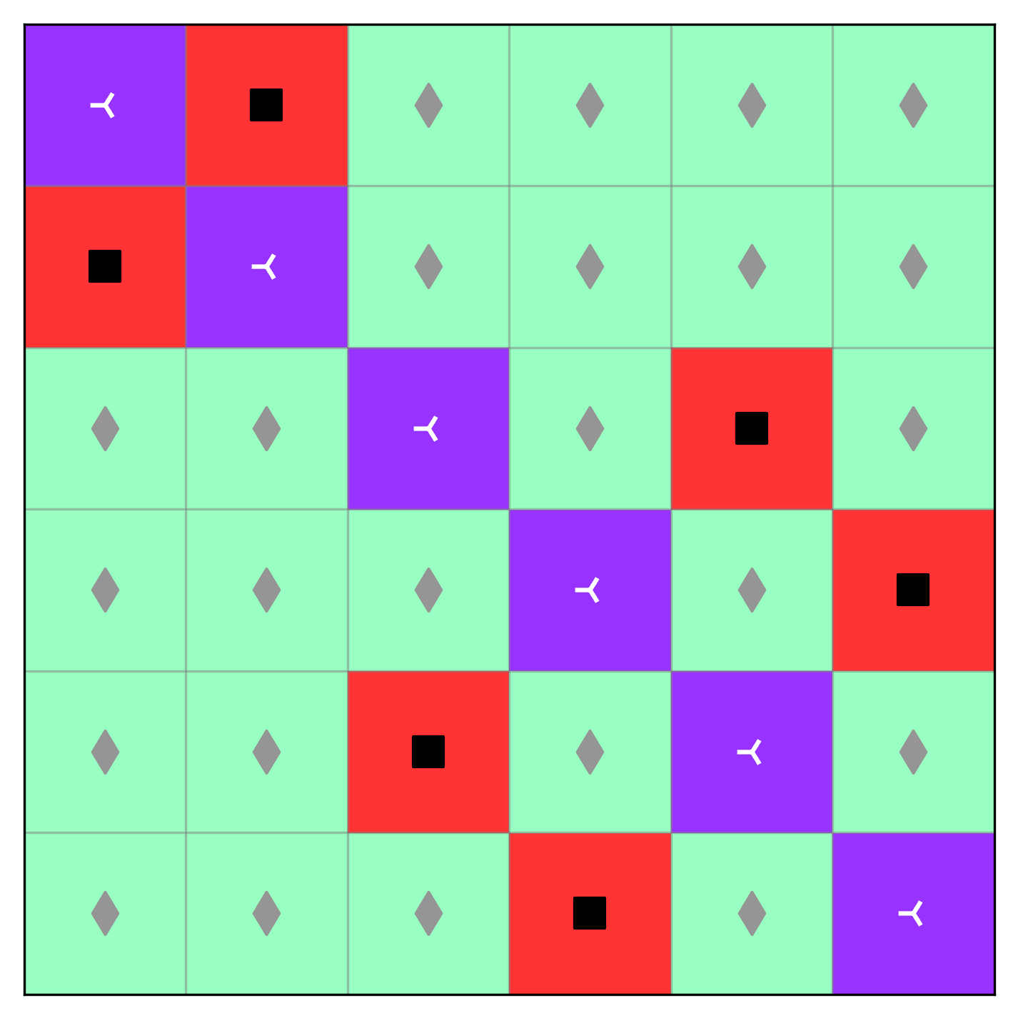
Figure 4: As we saw in Example 1 the rotational symmetries of the cube are given by ${H}={S}_{4}$. The action of this group on the 6 faces is the permutation group $\pi_{\Delta}({S}_{4})$. The parameter-sharing constraint for $6\times 6$ matrices $\textbf{{{L}}}_{H}$ is shown in this figure. The corresponding ${U}\wr{H}={G}$-equivariant map $\textbf{{{L}}}_{G}^{\text{hierarchy}}=\textbf{{{L}}}_{H}\otimes\left(1_{|{K}\times\Omega|}1_{|{K}\times\Omega|}^{\top}\right)+\textbf{{{I}}}_{|\Delta|}\otimes\textbf{{{L}}}_{U}$ assuming a $3\times 3$ face grid is constructed in two steps: 1) subdividing each row and column of $\textbf{{{L}}}_{H}$ into $3\times 3\times 4=28$ parts, to get a $216\times 216$ matrix for $\textbf{{{L}}}_{H}\otimes\left(1_{|{K}\times\Omega|}1_{|{K}\times\Omega|}^{\top}\right)$; 2) replacing the purple diagonal blocks with the $28\times 28$ parameter-sharing matrix of Fig. 3. This corresponds to the second term $\textbf{{{I}}}_{|\Delta|}\otimes\textbf{{{L}}}_{U}$.

4 Revisiting Gauge Equivariance

Cohen et al. (2019a) introduced gauge equivariant CNNs and used it to build Icosahedral CNN; an equivariant network for pixelization of the icosahedron. The idea is that a manifold as a geometric object may lack a global symmetry, and we can instead design models equivariant to the change of local symmetry, or gauge. To establish the relationship between their model and ours, in their language, we assume each face to be a local chart. The interaction between local charts or faces is only through their overlap created by the padding of each face from adjacent faces. If we ignore the padding, their framework assumes an “independent” local transformation within each chart – that is, their model is equivariant to independent translation and rotation/reflection within each face tiling. These independent transformations are represented by the product group ${U}_{1}\times\ldots\times{U}_{|\Delta|}$ acting on the set of all tiles $\Delta\times\Omega$, or $\Delta\times{K}\times\Omega$ in the case of regular features. Furthermore, since the “same” model applies across charts, gauge equivariance assumes exchangeability of these transformations. The resulting overall symmetry group is, therefore, the wreath product

$${G}={U}\wr{Sym}(\Delta)$$ (3)

in which a member of the symmetric group ${s}\in{S}_{|\Delta|}$ permutes the transformations ${u}_{1},\ldots,{u}_{|\Delta|}\in{U}_{1}\times\ldots\times{U}_{|\Delta|}$. Therefore, ${G}$ action on $\Delta\times{K}\times\Omega$ is given by the following

$$\bm{\rho}_{\Delta\times\Omega}^{\text{gauge}}{({g})}=\left(\bm{\sigma}_{\Delta}{({s})}\otimes\textbf{{{I}}}_{|{K}\times\Omega|}\right) \left(\bigoplus_{f\in\Delta}{\bm{\upsilon}_{{K}\times\Omega}}{({u}_{f})}\right),$$ (4)

where ${g}=({s},{u}_{1},\ldots,{u}_{|\Delta|})$. Here, the direct sum represents the independent transformation of each face by $\bm{\upsilon}({u}_{f})$ of Eq. 2, and the first term permutes the blocks in the direct sum using $\bm{\sigma}_{\Delta}({s})$. Action for scalar features simply replaces $\bm{\upsilon}_{{K}\times\Omega}$ with $\bm{\upsilon}_{\Omega}$.

4.1 Gauge Equivariant Linear Map

Previously we saw that ${K}\rtimes{T}={U}$-equivariant maps $\textbf{{{L}}}_{U}$ can be expressed using parameter-sharing linear layers. In (Zaheer et al., 2017) it is shown that ${Sym}(\Delta)$-equivariant maps take a simple form $\textbf{{{L}}}_{{S}(\Delta)}=w_{1}\textbf{{{I}}}_{|\Delta|}+w_{2}(1_{|\Delta|}1_{|\Delta|}^{\top})$, where $\textbf{{{I}}}_{c}$ is the $c\times c$ identity matrix, and $1_{c}=[1,\ldots,1]^{\top}$ is a column vector of length $c$. Given these components, as shown by (Wang et al., 2020), the equivariant map for the imprimitive action of their wreath product, as defined by Eq. 4 has the following form:

$$\textbf{{{L}}}_{G}^{\text{gauge}}=\textbf{{{L}}}_{S}\otimes\left(1_{|{K}\times\Omega|}1_{|{K}\times\Omega|}^{\top}\right)+\textbf{{{I}}}_{|\Delta|}\otimes\textbf{{{L}}}_{U}.$$ (5)

In words, the resulting linear map applies the same $\textbf{{{L}}}_{U}$ to each face tiling, and one additional operation pools over the entire set of pixels, multiplies the result by a scalar, and broadcasts back. If we ignore the single global pool-broadcast operation, the result which simply applies an identical equivariant map to each chart coincides with the model of (Cohen et al., 2019a).

5 Combining Local and Global Symmetries

5.1 Strict Hierarchy of Symmetries

The symmetry group of Eq. 3 ignores the symmetries of the solid ${H}$. However, adding ${H}$ seems easy: by simply replacing the representation $\sigma_{\Delta}({S})$ with $\pi_{\Delta}({H})$ in Eq. 4, we get a smaller permutation group $\rho^{\text{hierarchy}}({G})$ acting on $\Delta\times{K}\times\Omega$. Intuitively, this permutation group includes independent symmetry transformations of the tiling of each face while allowing the faces to be permuted according to the symmetries of the solid. The new permutation group is a subgroup of the old group: $\rho^{\text{hierarchy}}({G})<\rho^{\text{gauge}}({G})$, which means that the corresponding ${G}$-equivariant map is less constrained or more expressive. The new ${G}$-equivariant map $\textbf{{{L}}}_{G}^{\text{hierarchy}}$ simply replaces $\textbf{{{L}}}_{{S}}$ in Eq. 5 with $\textbf{{{L}}}_{H}$. Parameter-sharing layers equivariant to ${H}$-action on faces $\bm{\pi}({H})$ are easily constructed for different solids; see Fig. 4.

While this approach is an improvement over the previous model, it is still inaccurate in the sense that it allows rotation/reflection of each face via $\kappa_{\Omega}({K})$ independently of rotations/reflections of the solid through $\pi_{\Delta}({H})$. In principle, rotations/reflections of the solid completely determine the rotations/reflections of face tilings for all faces. Next, we find the symmetry transformation that respects this constraint and, by doing so, increase the expressivity of the resulting equivariant map.

5.2 Interaction of Global and Local Symmetries

Previously we observed that ${H}$ action completely defines rotations and reflections of each face-tiling. Therefore our task is to define the pixelization symmetries ${G}$ solely in terms of ${H}$ and translations of individual tilings ${T}$ (i.e., we drop ${K}$). Assuming independent translation within each face, we get the product group

$${{T}}^{|\Delta|}=\underbrace{{T}\times\ldots\times{T}}_{|\Delta|\;\mathrm{times}}.$$ (6)

To combine this symmetry with the polyhedral symmetry ${H}$ one should note that ${H}$ itself acts on ${{T}}^{|\Delta|}$ – e.g., when we rotate the cube, translations are permuted and rotated. Geometrically, it is easy to see that ${H}$ action on ${{T}}^{|\Delta|}$ is an automorphism – there is a bijection between translations before and after rotating the solid. Let $b:{H}\to{Aut}({{T}}^{|\Delta|})$ define an automorphism of ${{T}}^{|\Delta|}$ for each rotation/reflection ${h}\in{H}$ of the solid. Then, the combined “abstract” symmetry is the semi-direct product constructed using $b$ – that is,

$${G}={H}\rtimes_{b}{{T}}^{|\Delta|}.$$ (7)

Next, we define this group’s permutation action on regular feature-fields $\Delta\times{K}\times\Omega$ – specialization to scalar fields is straightforward. To formalize this action, we need to introduce two ideas: 1) system of blocks in permutation groups; 2) flags and their properties in Platonic solids.

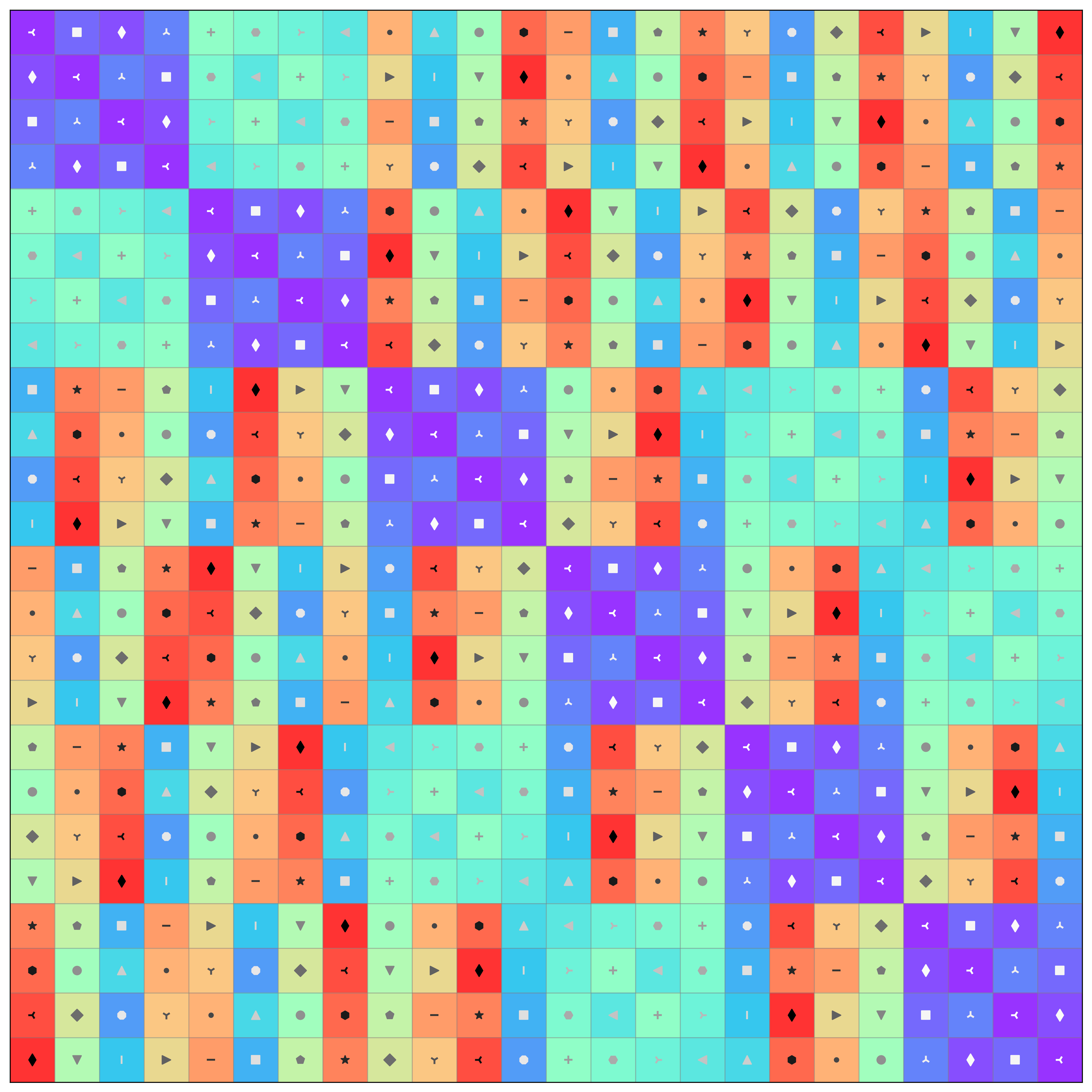
Figure 5: The parameter-sharing matrix for $\textbf{{{L}}}_{H}$, equivariant to $\pi_{\Delta\times{K}}({H})$ of Eq. 9; the rotations of the cube as they act on face-vertex pairs $\Gamma_{\text{chiral}}$. Since the cube has $6\times 4=24$ face-vertex pairs, this is a $24\times 24$ matrix. To obtain the operations of Eq. 11 for a quad sphere with $3\times 3$ tiling on each face, we need to repeat each row and column of this matrix $9$ ($=3\times 3$) times to get a $216\times 216$ matrix corresponding to $\textbf{{{L}}}_{H}\otimes({1}_{|\Omega|}{1}^{\top}_{|\Omega|})$. We then replace the $28\times 28$ purple blocks on the diagonal of the resulting matrix with identical copies of $\textbf{{{L}}}_{U}$ (Fig. 3); this corresponds to the second term $\textbf{{{I}}}_{|\Delta|}\otimes\textbf{{{L}}}_{U}$ in Eq. 11. The result is the parameter-sharing matrix of the equivariant map for a quad sphere, assuming regular features.

5.2.1 System of Blocks

Consider $\rho({G})<{Sym}(\Theta)$, the permutation action of some ${G}$ on a set $\Theta$. A block system is a partition of the set $\Theta$ into blocks $\mathrm{B}_{1}\cupdot\ldots\cupdot\mathrm{B}_{p}$ such that the action of ${G}$ preserves the block structure – that is $({g}\cdot\mathrm{B})\cap\mathrm{B}$ is either $\emptyset$ or $\mathrm{B}$ itself, where the dot indicates the group action. This means that for transitive sets we can identify the system of blocks using a single block $\mathrm{B}\subseteq\Theta$, and generate all the other blocks through ${G}$ action.

Let $Stab_{\rho}(\theta)<\rho({G})$ be the stabilizer subgroup for $\theta\in\Theta$; this is the subset of permutations in $\rho({G})$ that fix $\theta$. For the set $\mathrm{B}\subseteq\Theta$, let $Stab_{\rho}(\mathrm{B})<\rho({G})$ denote the set stabilizer subgroup – i.e., ${g}\cdot\mathrm{B}=\mathrm{B}$ for all ${g}\in Stab_{\bm{\rho}}(\mathrm{B})$. Given $\theta\in\Theta$, there is a bijection between subgroups of $\rho({G})$ that contain $Stab_{\rho}(\theta)$ and systems of block $\mathrm{B}\ni\theta$ (Dixon & Mortimer, 1996). In other words, any block system $\mathrm{B}\ni\theta$ can be identified with its set-stabilizer $Stab_{\rho}(\mathrm{B})$ which contains $Stab_{\rho}(\theta)$ as a subgroup. Given a block system $\mathrm{B}\subseteq\Theta$, we can decompose the permutation matrices $\bm{\rho}({g})$ as

$$\bm{\rho}({g})=\left(\bm{\rho}_{\Theta/\mathrm{B}}({g})\otimes\textbf{{{I}}}_{|\mathrm{B}|}\right)\left(\bigoplus_{\mathrm{B}}\bm{\rho}_{\mathrm{B}}({g})\right),$$ (8)

where $\bm{\rho}_{\Theta/\mathrm{B}}({g})$ permutes the blocks, and $\bm{\rho}_{\mathrm{B}}({g})\in Stab_{\rho}(\mathrm{B})$, permutes the elements inside the block $\mathrm{B}$. The reader may notice that the expression above resembles the wreath product action of Eq. 4. This is because the imprimitive action of the wreath product is a way of creating block systems in which one group permutes the blocks and independent action of a second group permutes each inner block – i.e., these groups act independently at the two levels of the hierarchy. However, to account for the interrelation between the global symmetry of the Platonic solid and the rotation/reflection symmetry of each face tiling, we need to consider the system of blocks created by ${H}$ action on flags.

5.2.2 Flags and Regular ${H}$-Action

Adjacent face-edge-vertex triples of polyhedra are called flags: $\Gamma=\{(f,e,v)\in[v]\times E\times\Delta\mid\{v\}\subset e\subset f\},$ where $E\subset[v]^{2}$ is the edgeset (Cromwell, 1999). An important property of Platonic solids is that their full symmetry group ${H}$ has a regular action on flags – i.e., a unique permutation in the permutation group $\pi_{\Gamma}({H})<{Sym}(\Gamma)$ moves one flag to another. If we consider only the rotational or chiral symmetries, the group action is regular on adjacent face-vertex pairs $\Gamma_{\mathrm{chiral}}=\{(f,v)\in[v]\times\Delta\mid v\in f\}$. Moving forward, we work with flags, having in mind that our treatment specializes to rotational symmetries by switching to $\Gamma_{\mathrm{chiral}}$.

5.2.3 ${G}$-Action and Equivariant Map

Now we have all the ingredients to define the ${G}$ action, for ${G}$ of Eq. 7, on the regular features of the pixelized sphere $\Delta\times{K}\times\Omega$. The subset of flags associated with a face $\Gamma(f)=\{(f,e,v)\in\Gamma\}\subset\Gamma$ form a block system under ${H}$ action – that is rotations/reflections of the solid keep the flags on the same face. Moreover, the set-stabilizer subgroup ${Stab}_{{\pi_{\Gamma}}}(\Gamma(f))$ that fixes a face, is isomorphic to rotation/reflection symmetries of the face-tiling ${Stab}_{\pi_{\Gamma}}(\Gamma(f))\cong{K}$ and so it has a regular action on features ${K}$. Therefore, we can decompose ${H}$ action on $\Gamma$ as Eq. 8

$${\bm{\pi}}_{\Gamma}({h})=\left(\bm{\pi}_{\Delta}({h})\otimes\textbf{{{I}}}_{|{K}|}\right)\left(\bigoplus_{f\in\Delta}\bm{\pi}_{\Gamma(f)}({h})\right),$$ (9)

where as before $\bm{\pi}_{\Delta}({h})$ permutes the faces, and $\bm{\pi}_{\Gamma(f)}({h})\in Stab_{\pi_{\Gamma}}(\Gamma(f))$ is a permutation of the flags of face $f$. Since $Stab_{\pi_{\Gamma}}(\Gamma(f))\cong{K}$, each $\bm{\pi}_{\Gamma(f)}({h})$ also uniquely identifies a rotation reflection of the tiling. Let $\bm{\pi}_{\Omega(f)}({h})<{Sym}(\Omega)$ denote this action on the tiling. The combined action of the polyhedral group ${H}$ on the pixelization is given by

$$\bm{\beta}({h})=\left(\bm{\pi}_{\Delta}({h})\otimes\textbf{{{I}}}_{|\Omega\times{K}|}\right)\left(\bigoplus_{f\in\Delta}\bm{\pi}_{\Gamma(f)}({h})\otimes\left(\bm{\pi}_{\Omega(f)}({h})\right)\right).$$

When defining the abstract symmetry of the solid we noted that the polyhedral group defines an automorphism of translations $b_{h}:{{T}}^{|\Delta|}\to{{T}}^{|\Delta|}$. $\beta({H})$ concretely defines this automorphism through conjugation, resulting in the overall ${G}$ action:

$$\bm{\rho}^{*}({g})=\underbrace{\bm{\beta}({h})\left(\bigoplus_{f}\bm{\tau}(t_{f})\otimes\textbf{{{I}}}_{{K}}\right)\bm{\beta}({h})^{-1}}_{\text{automorphism $b_{h}$}}\bm{\beta}({h})$$ (10)

$$=\left(\bm{\pi}_{\Delta}({h})\otimes\textbf{{{I}}}_{|\Omega\times{K}|}\right)\left(\bigoplus_{f\in\Delta}\bm{\pi}_{\Gamma(f)}({h})\otimes\left(\bm{\pi}_{\Omega(f)}({h})\bm{\tau}({t}_{f})\right)\right),$$

where ${g}=({h},{t}_{1},\ldots{t}_{|\Delta|})$. Here, $\beta({H})$ transforms the translations, while also acting on $\Delta\times{K}\times\Omega$ (this is similar to Eq. 1). The end result is that the combination $\bm{\pi}_{\Omega(f)}({h})\bm{\tau}({t}_{f})$ performs translation followed by rotation/reflection on all tilings associated with a face, and $\bm{\pi}_{\Gamma(f)}({h})$ permutes the tilings associated with flags of face $f$.

The general form of $\rho^{*}$ is similar to $\rho^{\text{gauge}}$ of Eq. 4. The difference is that in that case we assumed arbitrary shuffling of charts (${s}\in{S}$) as well as independent rotations/reflections of each face (${k}_{f}\in{K}$). Therefore we have ${g}=({s},({t}_{1},{k}_{1}),\ldots,({t}_{|\Delta|},{k}_{|\Delta|}))$. In our approach, $\sigma({S})$ is replaced by $\pi({H})$, and all rotations/reflections ${k}_{f}$ for $f\in\Delta$ are dictated by $\bm{\pi}$ as well - therefore we have ${g}=({h},{t}_{1},\ldots{t}_{|\Delta|})$. As a permutation group we have

$$\rho^{*}<\rho^{\text{hierarchy}}<\rho^{\text{gauge}}<{Sym}(\Delta\times{K}\times\Omega).$$

Next, we express the equivariant map for the pixelized sphere in terms of the equivariant map for the polyhedral group and the equivariant map for the face tiling.

Claim 1.

Let $\textbf{{{L}}}_{H}:\mathds{R}^{|\Gamma|}\to\mathds{R}^{|\Gamma|}$ be equivariant to ${H}$-action $\pi_{\Gamma}({H})$. Similarly, assume $\textbf{{{L}}}_{{U}}:\mathds{R}^{|{K}\times\Omega|}\to\mathds{R}^{|{K}\times\Omega|}$ is equivariant to $\upsilon_{{K}\times\Omega}({U})$ as defined in Eq. 2. Then the linear map $$\textbf{{{L}}}_{G}=\textbf{{{L}}}_{H}\otimes({1}_{|\Omega|}{1}^{\top}_{|\Omega|})+\textbf{{{I}}}_{|\Delta|}\otimes\textbf{{{L}}}_{U}$$ (11) is equivariant to ${G}$ action of Eq. 2. The proof is in Appendix A. Note that while the form of the equivariant map resembles the equivariant map for the hierarchy of symmetries (e.g., Eq. 5), here we do not have a strict hierarchy; See Fig. 5 for the example of the quad sphere.

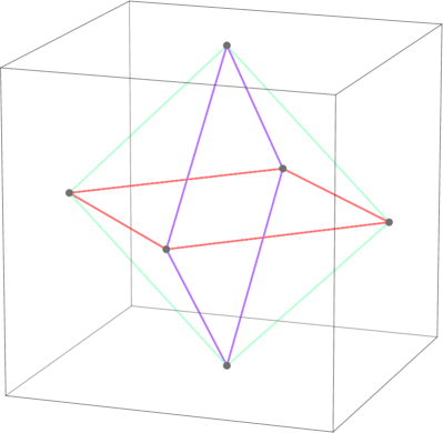
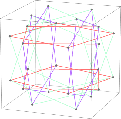
Figure 6: Padding graphs for our running example of quad sphere assuming rotational symmetry. Edge colors are added only to aid visualization. (Left) scalar features: the graph shows the neighborhood structure of faces. (Right) regular features: each face-vertex pair (a face corner) identifies a $\gamma\in\Gamma_{\text{chiral}}$. In both cases, the graphs are invariant under the action of ${H}$, which rotates the cube, where the group acts on the nodes of the padding graph.

5.3 Orientation Awareness

For some tasks, the spherical data may have a natural orientation. For example, in omnidirectional images, there is a natural up and down. In this case, equivariance to all rotations of the sphere over-constrains the model. A simple way to handle orientation in our equivariant map is to change $\textbf{{{L}}}_{H}$ to $\textbf{{{L}}}_{{H}^{\prime}}$ where $\pi({H}^{\prime})<\pi({H})$ is the subgroup that corresponds to the desired symmetry. In the example of omnidirectional camera, when using a quad sphere, ${H}^{\prime}={C}_{4}$, and its action $\pi({H}^{\prime})$ corresponds to rotations around the vertical axis.

5.4 Equivariant Padding

Our goal is to define padding of face tilings for both scalar and regular features. For scalar features, it is visually clear which pixels are neighbors, and it is easy to produce such a padding operation. However, for regular features, where we have one tiling $\Omega(\gamma)$ per flag $\gamma\in\Gamma$, padding is more challenging. Below we give a procedure. Padding is a set of pairs $\Lambda\subset\Gamma\times\Gamma$ that identify neighboring flags. Since this neighborhood is symmetric, padding can also be interpreted as an undirected graph. Padding $\Lambda$ should satisfy the following two conditions: i) each pair belong to neighboring faces; ii) $\Lambda$ is equivariant to ${H}$ action:

$$adj(\Lambda)\;\bm{\pi}_{\Delta\times{K}}({h})=\bm{\pi}_{\Delta\times{K}}({h})\;adj(\Lambda)\quad\forall{h}\in{H},$$ (12)

where $adj(\Lambda)\in\{0,1\}^{|\Gamma|\times|\Gamma|}$ is the adjacency matrix of the padding graph. In other words, $\pi({H})$ defines the automorphisms of the padding graph; see Fig. 6 for an example. Our equivariant padding resembles ${G}$-padding of (Cohen et al., 2019a); however, it is built using the high-level symmetry of the solid rather than relying on the choice of gauge in neighboring faces.

5.5 Efficient Implementation

We build equivariant networks by stacking equivariant maps and $\mathrm{ReLU}$ nonlinearity: $\textbf{{{L}}}_{{G}}^{(\ell)}\circ\mathrm{ReLU}\ldots\circ\mathrm{ReLU}\circ\textbf{{{L}}}_{{G}}^{(1)}$. Invariant networks use additional global average pooling in the end. For implementing $\textbf{{{L}}}_{G}$ of Eq. 11, we need efficient implementations of both terms in that equation. We implement the first term in Eq. 11 using an efficient combination of Pool-Broadcast operations:

$$\textbf{{{L}}}_{{H}}\otimes(1_{|\Omega|}1^{\top}_{|\Omega|})=\mathrm{Broadcast}_{\Omega}\circ\textbf{{{L}}}_{H}\circ\mathrm{Pool}_{\Omega}.$$

In words, we first pool over each tiling $\Omega(\gamma)\;\forall\gamma\in\Gamma$, then apply the parameter-sharing layer $\textbf{{{L}}}_{H}$, and broadcast the result back to pixels $\Omega(\gamma)$. To implement $\textbf{{{L}}}_{H}$, we use the parameter-sharing library mentioned earlier

For triangular faces, we would like each pixel to be able to be translated to any other pixel. Therefore, we consider the input signal to lie only on downward-facing triangles. This is equivalent to considering a hexagonal grid of pixels; see Fig. 7. We use implementations of group convolution for both square and hexagonal grids (Cohen & Welling, 2016; Hoogeboom et al., 2018).

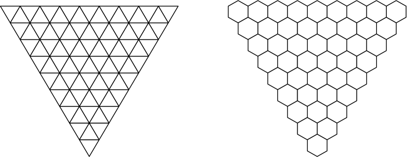
Figure 7: A triangular tiling is converted to a hexagonal tiling by replacing each down-facing triangle with a hexagon.

6 Related Works

Our contribution is related to a large body of work in equivariant and geometric deep learning. In design of equivariant networks one could either find equivariant linear bases (Wood & Shawe-Taylor, 1996) or alternatively use group convolution (Cohen et al., 2019b); these approaches are equivalent (Ravanbakhsh, 2020). For permutation groups the first perspective leads to parameter-sharing layers (Ravanbakhsh et al., 2017) that are used in deep learning with sets (Zaheer et al., 2017; Qi et al., 2017), tensors (Hartford et al., 2018), and graphs (Kondor et al., 2018b; Maron et al., 2019), where the focus has been on the symmetric group. The group convolution approach which has been formalized in a series of works (Cohen & Welling, 2017; Kondor & Trivedi, 2018; Cohen et al., 2019b; Lang & Weiler, 2021) has been mostly applied to exploit subgroups of the Euclidean group. Among many papers that explore equivariance to Euclidean isometries are (Marcos et al., 2017; Worrall et al., 2017; Thomas et al., 2018; Bekkers et al., 2018; Weiler et al., 2018; Weiler & Cesa, 2019). Some of the papers that more specifically consider the subgroups of the orthogonal group are (Cohen et al., 2018; Esteves et al., 2018; Perraudin et al., 2019; Anderson et al., 2019; Bogatskiy et al., 2020; Dym & Maron, 2020). Other notable approaches include capsule networks (Sabour et al., 2017; Lenssen et al., 2018), equivariant attention mechanisms, and transformers (Fuchs et al., 2020; Romero et al., 2020; Hutchinson et al., 2020; Romero & Cordonnier, 2021).

The gauge equivariant framework of (Cohen et al., 2019a) further extends the group convolution formalism, and it has been applied to spherical data as well as 3D meshes (Haan et al., 2021). In addition to their model for the pixelized sphere, discussed in section Section 4, the same framework is used to create a model for irregularly sampled points in Kicanaoglu et al. (2020). Equivariant networks using global symmetries of geometric objects such as mesh and polyhedra that assume complete exchangeability of the nodes are studied in (Albooyeh et al., 2020).

Table 1: Results for different symmetry assumptions (no padding). Pixel densities in figures match those of the experiments.

	Tetetrahedron	Cube	Octahedron	Icosahedron
$|\Delta|$	4	6	8	20
$|\Omega|$	861	576	325	153
${H}$	$A_{4}$	$S_{4}$	$S_{4}$	$A_{5}$
Using different number of channels for the global operations $\textbf{{{L}}}_{H}$ in the final model
25%	$98.79\pm 0.03$	$98.94\pm 0.09$	$98.96\pm 0.08$	$98.82\pm 0.07$
50%	$98.73\pm 0.08$	$98.99\pm 0.05$	$99.02\pm 0.05$	$98.93\pm 0.11$
75%	$98.70\pm 0.10$	$98.88\pm 0.04$	$99.00\pm 0.06$	$98.76\pm 0.10$
100%	$98.72\pm 0.09$	$98.83\pm 0.05$	$98.95\pm 0.07$	$98.84\pm 0.06$
Comparison of different models
Gauge (${U}\wr{Sym}(\Delta)$) - Section 4	$98.37\pm 0.07$	$98.70\pm 0.06$	$98.25\pm 0.11$	$97.45\pm 0.12$
Hierarchical (${U}\wr{H}$) - Section 5.1	$98.62\pm 0.10$	$98.82\pm 0.03$	$98.62\pm 0.03$	$98.54\pm 0.05$
Our Final Model (${H}\rtimes{{T}}^{|\Delta|}$) - Section 5.2	$98.73\pm 0.08$	$98.99\pm 0.05$	$99.02\pm 0.05$	$98.93\pm 0.11$

Below we quickly review other equivariant and non-equivariant models that are specialized for spherical data. Boomsma & Frellsen (2017) model the sphere as a cube and apply 2D convolution on each face with no parameter-sharing across faces. Su & Grauman (2017) and Coors et al. (2018) design spherical CNNs for the task of omnidirectional vision. They use oriented convolution filters that transform according to the distortions produced by the projection method. Esteves et al. (2018) define a spherical convolution layer that operates in the spectral domain. Their model is $SO(3)$ equivariant, and their convolution filters are isotropic and non-localized.

Cohen et al. (2018) define an equivariant spherical correlation operation in $SO(3)$ which is further improved by Kondor et al. (2018a) who introduce a Fourier-space nonlinearity and by Cobb et al. (2021) who make it more efficient. This enables them to implement the whole neural network in the Fourier domain. Jiang et al. (2019) define convolution on unstructured grids via parameterized differential operators. They apply this convolution layer to the icosahedral spherical mesh (icosphere grid). Liu et al. (2018) introduce alt-az spherical convolution, which is equivariant to azimuth rotations, and implement it on the icosphere grid.

Zhang et al. (2019) model the sphere as an icosahedron. They unwrap the icosahedron and convolve it with a hexagonal kernel in two orientations. They then interpolate the result of the two convolutions to obtain a north-aligned convolution layer for the sphere. Defferrard et al. (2020) build a graph on top of a discrete sampling of the sphere and then process this graph with an isotropic graph CNN. This is similar to using a gauge equivariant network with scalar feature maps. Esteves et al. (2020) define $SO(3)$ equivariant convolution between spin weighted spherical functions. Their convolutional filters are anisotropic and non-localized. Similar to Esteves et al. (2018), they make the filters more localized via spectral smoothness.

Table 2: Spherical MNIST result.

Method	Acc. (%)
Esteves et al. (2018)	98.72
Cohen et al. (2018)	99.12
Cohen et al. (2019a)	99.31
Esteves et al. (2020)	99.37
Kicanaoglu et al. (2020)	99.43
Ours (cube + padding)	99.42

7 Experiments

We use the efficient implementation of Section 5.5 in all experiments. Details of training and architectures appear in Appendix D and Appendix E. Below, we report our experimental results on spherical MNIST, Stanford 2D3DS, and HAPPI20 climate data.

7.1 Spherical MNIST

The spherical MNIST dataset (Cohen et al., 2018) consists of images from the MNIST dataset projected onto a sphere with random rotation. We consider the setting in which both training and test images are randomly rotated. As seen in Table 2, our quad sphere model is able to compete with state-of-the-art.

Next, we study the effect of our global equivariant operation $\textbf{{{L}}}_{H}$ that depends on the symmetry of the solid, as well as the effect of the choice of solid. For these experiments, we do not use equivariant padding. We transform the dataset into our polyhedral sphere representation with the use of bilinear interpolation. Table 1 visualizes different pixelizations and reports the choice of group ${H}$ (for rotational symmetries) and the number of pixels per face $|\Omega|$. Since the number of parameters in $\textbf{{{L}}}_{H}$ becomes large when we have multiple channels, we allow for a fraction of channels to use $\textbf{{{L}}}_{H}$. The remaining channels only have local operations $\textbf{{{L}}}_{U}$. The first four rows of Table 1 show this fraction’s effect on the performance. Overall, we observe that using a fraction of channels for $\textbf{{{L}}}_{H}$ improves the model’s performance.

We then compare the performance of the three models discussed in Sections 4, 5.1 and 5.2, where from top to bottom the size of the symmetry group decreases, and therefore we expect the model to become more expressive. The results are in agreement with this expectation. Interestingly, in polyhedra with more faces, the effect of using more expressive global operations is generally more significant – e.g., for the icosahedron, the improvement is larger than that of the tetrahedron.

We choose to use the cube for the following experiments because of the simplicity and efficiency of its implementation and its good performance.

Table 3: Results on Stanford 2D3DS.

	Method	Mean Acc. (%)	Mean IoU (%)
non-oriented	Cohen et al. (2019a)	55.9	39.4
	Kicanaoglu et al. (2020)	58.2	39.7
	Esteves et al. (2020)	55.65	41.95
	Ours (cube)	58.74	40.99
oriented	Jiang et al. (2019)	54.7	38.3
	Zhang et al. (2019)	58.6	43.3
	Ours (cube + orientation)	62.5	45.0

7.2 Omnidirectional Camera Images

The Stanford 2D3DS dataset (Armeni et al., 2017) consists of 1413 omnidirectional RGBD images from 6 different areas. The task is to segment the images into 13 semantic categories. We use the standard 3-fold cross-validation split and calculate average accuracy and IoU for each class over different splits. Then, we average the metrics obtained for each class to obtain an overall metric for this dataset. We compose our equivariant map and equivariant padding in a U-Net architecture (Ronneberger et al., 2015). Because of class imbalance, we use a weighted loss similar to previous works - e.g., Jiang et al. (2019). Our oriented model, described in Section 5.3, achieves state-of-the-art performance on this dataset; See Table 3.

7.3 Climate Data

We apply our model to the task of segmenting extreme climate events (Mudigonda et al., 2017). We use climate data produced by the Community Atmospheric Model v5 (CAM5) global climate simulator, specifically, the HAPPI20 run. The training, validation, and test set size is 43917, 6275, and 12549, respectively. The input consists of 16 feature maps. We normalize each channel of the input to have zero mean and unit standard deviation. The task is to segment atmospheric rivers (AR) and tropical cyclones (TC). The rest of the pixels are labeled as background (BG). See Mudigonda et al. (2017) for how ground truth labels are generated for this dataset. The classes are heavily unbalanced with $0.1\%$ TC, $2.2\%$ AR, and $97.7\%$ BG. To account for this unbalance, we use a weighted cross-entropy loss. We project the input features onto a quad sphere with $48\times 48$ pixels/face. We use the non-oriented model for this task. In our experiments, we observed no significant gain from using the oriented model. Experimental results can be seen in Table 4. Our method achieves the highest accuracy and average precision.

Table 4: Results on HAPPI20: mean accuracy (over TC, AR, BG) and mean average precision (over TC and AR).

Method	Mean Acc. (%)	Mean AP (%)
Jiang et al. (2019)	94.95	38.41
Zhang et al. (2019)	97.02	55.5
Cohen et al. (2019a)	97.7	75.9
Defferrard et al. (2020)	97.8 $\pm$ 0.3	77.15 $\pm$ 1.94
Kicanaoglu et al. (2020)	97.1	80.6
Ours (cube)	99.30	95.20

Conclusion

This paper introduces a family of equivariant maps for Platonic pixelizations of the sphere. The construction of these maps combines the polyhedral symmetry with the rotation/reflection symmetry of their face-tiling. The latter is then, in turn, combined with the translational symmetry of pixels on each face to produce an overall permutation group. Our use of system of blocks to formalize this transformation merits further exploration as it provides a generalization of a hierarchy of symmetries. Our derivation also demonstrates a close connection to gauge equivariant CNNs and suggests a generalization in settings where local charts possess a higher-level symmetry. Our equivariant maps, which have efficient implementations, are combined with an equivariant padding procedure to build deep equivariant networks. These networks achieve state-of-the-art results on several benchmarks. Given the ubiquitous nature of spherical data, we hope that our contributions will lead to a broad impact.

Appendix A Proof

Proof.

of 1
Our assumptions give us the following equivariance conditions:

$$\textbf{{{L}}}_{U}\bm{\upsilon}_{{K}\times\Omega}({u}) =\bm{\upsilon}_{{K}\times\Omega}({u})\textbf{{{L}}}_{U}\quad \forall{u}\in{U}$$ (13)

$$\textbf{{{L}}}_{H}\bm{\pi}_{\Delta\times{K}}({h}) =\bm{\pi}_{\Delta\times{K}}({u})\textbf{{{L}}}_{U}\quad \forall{h}\in{H}$$ (14)

Our goal is to show that

$$\bm{\rho}^{*}({g})\textbf{{{L}}}_{G}=\textbf{{{L}}}_{G}\bm{\rho}^{*}({g})\forall{g}\in{G},$$ (15)

for $\bm{\rho}^{*}({g})$ of Eq. 10. We do this in two parts.

Part 1.

First we show $\textbf{{{I}}}_{|\Delta|}\otimes\textbf{{{L}}}_{U}$ commutes with $\bm{\rho}^{*}({g})$. From Eq. 13, using Eq. 2, and since ${K}\cong Stab_{\pi_{\Gamma}}(\Gamma(f))$ we have $\forall{h}\in{H},f\in\Delta$

$$\textbf{{{L}}}_{U}\left(\bm{\pi}_{\Gamma(f)}({h})\otimes\bm{\pi}_{\Omega(f)}({h})\bm{\tau}({t}_{f})\right)=$$

$$\quad\left(\bm{\pi}_{\Gamma(f)}({h})\otimes\bm{\pi}_{\Omega(f)}({h})\bm{\tau}({t}_{f})\right)\textbf{{{L}}}_{U}\quad$$ (16)

Since $\bm{\pi}_{\Gamma(f)}({h})\otimes\bm{\pi}_{\Omega(f)}({h})\bm{\tau}({t}_{f})=\bm{\upsilon}_{\Delta\times{K}}({u})$ for some ${u}\in{U}$, we use the short notation

$$\bm{\upsilon}_{\Delta\times{K}}(f,{h})\doteq\bm{\pi}_{\Gamma(f)}({h})\otimes\bm{\pi}_{\Omega(f)}({h})\bm{\tau}({t}_{f}).$$

In this notation, we can rewrite $\bm{\rho}^{*}({g})$ as

$$\bm{\rho}^{*}({g})=\left(\bm{\pi}_{\Delta}({h})\otimes\textbf{{{I}}}_{|\Omega\times{K}|}\right)\left(\bigoplus_{f\in\Delta}\bm{\upsilon}_{\Delta\times{K}}(f,{h})\right)$$ (17)

Commutativity of $\textbf{{{I}}}_{|\Delta|}\otimes\textbf{{{L}}}_{U}$ and $\bm{\rho}^{*}({g})$ follows from Eq. 16 and the fact that the identity matrix commutes with any other matrix gives:

$$\overbrace{\left(\bm{\pi}_{\Delta}({h})\otimes\textbf{{{I}}}_{|\Omega\times{K}|}\right)\left(\bigoplus_{f\in\Delta}\bm{\upsilon}_{\Delta\times{K}}(f,{h})\right)}^{\bm{\rho}^{*}({g})}\left(\textbf{{{I}}}_{|\Delta|}\otimes\textbf{{{L}}}_{U}\right)$$

$$= \left(\bm{\pi}_{\Delta}({h})\otimes\textbf{{{I}}}_{|\Omega\times{K}|}\right)\left(\textbf{{{I}}}_{|\Delta|}\otimes\textbf{{{L}}}_{U}\right)\left(\bigoplus_{f\in\Delta}\bm{\upsilon}_{\Delta\times{K}}(f,{h})\right)$$

$$= \left(\textbf{{{I}}}_{|\Delta|}\otimes\textbf{{{L}}}_{U}\right)\underbrace{\left(\bm{\pi}_{\Delta}({h})\otimes\textbf{{{I}}}_{|\Omega\times{K}|}\right)\left(\bigoplus_{f\in\Delta}\bm{\upsilon}_{\Delta\times{K}}(f,{h})\right)}_{\bm{\rho}^{*}({g})}$$

where in the second line, we used the fact that two block diagonal matrices with the same block sizes commute if corresponding blocks commute. To get the final equality we twice used the mixed product property of tensor product $(\textbf{{{A}}}\otimes\textbf{{{B}}})(\textbf{{{C}}}\otimes\textbf{{{D}}})=(\textbf{{{A}}}\textbf{{{C}}})\otimes(\textbf{{{B}}}\textbf{{{D}}})$:

$$\left(\textbf{{{I}}}_{|\Delta|}\otimes\textbf{{{L}}}_{U}\right)\left(\bm{\pi}_{\Delta}({h})\otimes\textbf{{{I}}}_{|\Omega\times{K}|}\right)$$

$$= \left(\textbf{{{I}}}_{|\Delta|}\bm{\pi}_{\Delta}({h})\right)\otimes\left(\textbf{{{L}}}_{U}\textbf{{{I}}}_{|\Omega\times{K}|}\right)$$

$$= \left(\bm{\pi}_{\Delta}({h})\textbf{{{I}}}_{|\Delta|}\right)\otimes\left(\textbf{{{I}}}_{|\Omega\times{K}|}\textbf{{{L}}}_{U}\right)$$

$$= \left(\bm{\pi}_{\Delta}({h})\otimes\textbf{{{I}}}_{|\Omega\times{K}|}\right)\left(\textbf{{{I}}}_{|\Delta|}\otimes\textbf{{{L}}}_{U}\right)$$

Part 2.

Next we show $\textbf{{{L}}}_{H}\otimes({1}_{|\Omega|}{1}^{\top}_{|\Omega|})$ commutes with $\bm{\rho}^{*}({g})$. For this, we need to decompose the second part of $\bm{\rho}^{*}({g})$ of Eq. 10. We use the following property of tensor product $\textbf{{{A}}}\otimes\textbf{{{B}}}=(\textbf{{{A}}}\otimes\textbf{{{I}}})(\textbf{{{I}}}\otimes\textbf{{{B}}})$, and the block-diagonal structure produced by direct sum to rewrite $\bm{\rho}^{*}({g})$ as

$$\bm{\rho}^{*}({g})= \overbrace{\left(\bm{\pi}_{\Delta}({h})\otimes\textbf{{{I}}}_{|\Omega\times{K}|}\right)\left(\bigoplus_{f\in\Delta}\bm{\pi}_{\Gamma(f)}({h})\otimes\textbf{{{I}}}_{|\Omega|}\right)}^{(i)}$$ (18)

$$\underbrace{\left(\bigoplus_{f\in\Delta}\textbf{{{I}}}_{|{K}|}\otimes\left(\bm{\pi}_{\Omega(f)}({h})\bm{\tau}({t}_{f})\right)\right)}_{(ii)}.$$

Next, we show that each of the terms (i), and (ii) above commutes with $\textbf{{{L}}}_{H}\otimes({1}_{|\Omega|}{1}^{\top}_{|\Omega|})$. First, rewrite (i) using Eq. 8 to get

$$\overbrace{\left(\bm{\pi}_{\Gamma}({h})\otimes\textbf{{{I}}}_{|\Omega|}\right)}^{(i)}\left(\textbf{{{L}}}_{H}\otimes({1}_{|\Omega|}{1}^{\top}_{|\Omega|})\right)$$ (19)

$$= \left(\bm{\pi}_{\Gamma}({h})\textbf{{{L}}}_{H}({1}_{|\Omega|}\right)\otimes\left(\textbf{{{I}}}_{|\Omega|}({1}_{|\Omega|}{1}^{\top}_{|\Omega|})\right)$$ (20)

$$= \left(\textbf{{{L}}}_{H}({1}_{|\Omega|}\bm{\pi}_{\Gamma}({h})\right)\otimes\left(({1}_{|\Omega|}{1}^{\top}_{|\Omega|})\textbf{{{I}}}_{|\Omega|}\right)$$ (21)

$$= \left(\textbf{{{L}}}_{H}\otimes({1}_{|\Omega|}{1}^{\top}_{|\Omega|})\right)\left(\bm{\pi}_{\Gamma}({h})\otimes\textbf{{{I}}}_{|\Omega|}\right)$$ (22)

We then use the fact that (ii) is block-diagonal with $|\Delta\times{K}|$ blocks, and $({1}_{|\Omega|}{1}^{\top}_{|\Omega|})$ commutes with any matrix to show commutativity:

$$\left(\bigoplus_{f\in\Delta}\textbf{{{I}}}_{|{K}|}\otimes\left(\bm{\pi}_{\Omega(f)}({h})\bm{\tau}({t}_{f})\right)\right)\left(\textbf{{{L}}}_{H}\otimes({1}_{|\Omega|}{1}^{\top}_{|\Omega|})\right)$$ (23)

$$= \left(\bigoplus_{f,{k}\in\Delta\times{K}}\left(\bm{\pi}_{\Omega(f)}({h})\bm{\tau}({t}_{f})\right)\right)\left(\textbf{{{L}}}_{H}\otimes({1}_{|\Omega|}{1}^{\top}_{|\Omega|})\right)$$ (24)

$$= \left(\textbf{{{L}}}_{H}\otimes({1}_{|\Omega|}{1}^{\top}_{|\Omega|})\right)\left(\bigoplus_{f,{k}\in\Delta\times{K}}\left(\bm{\pi}_{\Omega(f)}({h})\bm{\tau}({t}_{f})\right)\right)$$ (25)

$$\left(\textbf{{{L}}}_{H}\otimes({1}_{|\Omega|}{1}^{\top}_{|\Omega|})\right)\left(\bigoplus_{f\in\Delta}\textbf{{{I}}}_{|{K}|}\otimes\left(\bm{\pi}_{\Omega(f)}({h})\bm{\tau}({t}_{f})\right)\right).$$ (26)

Parts 1. and 2. together complete the proof. ∎

Appendix B Equivariant Padding for the Cube

Fig. 8 shows how a face of the cube is padded when we have scalar features. Fig. 9 shows equivariant padding of a face in the more challenging case of regular features. Here we have one tiling $\Omega(\gamma)$ for each $\gamma\in\Gamma_{\text{chiral}}$ – i.e., one regular grid per face-vertex pair. We have visualized these grids by putting them close to a corner. We pad the corner pixels with zero.

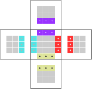
Figure 8: Equivariant padding applied to a single face of the cube in the setting where there is one grid per face.

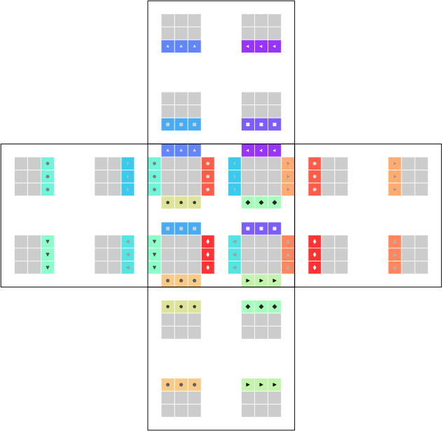
Figure 9: An example of an equivariant padding applied to a single face of the cube. The top left feature grid is matched to the top left feature grids of neighboring faces, the top right feature grid is matched to the top right feature grids of neighboring faces, and so on. The complete padding operation consists of applying this operation to each face of the cube. One can verify equivariance by noting that rotation followed by padding is equivalent to padding followed by rotation.

Appendix C Hexagonal Pooling

It is common for CNNs to include pooling layers that reduce the spatial dimension of internal representations. Fig. 10 shows how the pooling layer operates on a hexagonal grid. Pooling changes the width from $w$ to $(w+1)/2$. Since there are three pooling layers in our neural network architectures (see Appendix E), the initial width of the hexagonal grid has to be of the form $8k+1$.

Figure 10: Two instances of a hexagonal pooling filter in action. The colored pixels on the left are being pooled over to produce the colored pixel on the right.

Appendix D Details of Experiments

We implemented our models with PyTorch. We use the Adam optimizer in all experiments. The width of the platonic pixelizations are chosen such that pooling can be applied three times and the number of pixels is comparable to previous works (e.g., Jiang et al. (2019)).

D.1 Classification

We use the CNN architecture of Section E.1 for classification. Hyperparameters C and F (defined in Appendix E) are set to $20$ and $0.25$ respectively. Rate of dropout is set to $0.333$. We use a batch size of $128$. The model is trained for $50$ epochs with an initial learning rate of $10^{-3}$ that is multiplied by $0.1$ every $20$ epochs. Training a model takes near 3 hours on a V100 GPU.

D.2 Segmentation

We use the U-Net architecture described in Section E.2 for the two segmentation tasks. The models were trained with an initial learning rate of $3\cdot 10^{-3}$ that is multiplied by $0.7$ every $20$ epochs.

D.2.1 Stanford2D3DS

The hyperparameters C and F were set to $16$ and $0.2$ respectively. We used a batch size of $16$ and a dropout rate of $0.333$. The model was trained for $120$ epochs. Training a model the three cross-validation splits takes near 4 hours on a Quadro RTX 8000 GPU.

D.2.2 HAPPI20

The class weights used in the weighted cross-entropy loss are $0.00766805$, $0.94184578$, and $0.05048618$ for BG, TC, and AR respectively. The hyperparameter C was set to $28$ and F was set to $0.5$. We used a batch size of $64$ and a dropout rate of $0.1$. The model is trained until no improvement in validation performance is observed for $30$ epochs. Training a model takes near 3 days on two V100 GPUs.

Appendix E Neural Network Architecture

The layers inside Sequential are applied sequentially. SphereLayer is the hierarchical sphere layer introduced in this paper. It consists of GroupConv and PoolPolyBroadcast which pools each grid, applies an ${H}$-equivariant layer, and broadcasts the result back on the grids. PolyPad is the equivariant padding layer described in Section 5.4.

E.1 Classification

Sequential(  PolyPad(poly=POLY, padding=1)  GroupConv(in_channels=1, out_channels=C, kernel_size=3)  AssertShape(BATCH_SIZE, NUM_FACES, C, NUM_FLAGS_PER_FACE, WIDTH, WIDTH)  BatchNorm, ReLU, Dropout  PolyPad(poly=POLY, padding=1)  GroupConv(in_channels=C, out_channels=C, kernel_size=3)  BatchNorm, ReLU, Dropout  PolyPad(poly=POLY, padding=1)  SphereLayer(    PoolPolyBroadcast(poly=POLY, in_channels=C * F, out_channels=C * F)    GroupConv(in_channels=C, out_channels=C, kernel_size=3)  )  MaxPool(kernel_size=2, stride=2)  GroupConv(in_channels=C, out_channels=2 * C, kernel_size=1)  BatchNorm, ReLU, Dropout  PolyPad(poly=POLY, padding=1)  GroupConv(in_channels=2 * C, out_channels=2 * C, kernel_size=3)  BatchNorm, ReLU, Dropout  PolyPad(poly=POLY, padding=1)  SphereLayer(    PoolPolyBroadcast(poly=POLY, in_channels=2 * C * F, out_channels=2 * C * F)    GroupConv(in_channels=2 * C, out_channels=2 * C, kernel_size=3)  )  MaxPool(kernel_size=2, stride=2)  GroupConv(in_channels=2 * C, out_channels=4 * C, kernel_size=1)  BatchNorm, ReLU, Dropout  GroupConv(in_channels=4 * C, out_channels=4 * C, kernel_size=3)  BatchNorm, ReLU, Dropout  PolyPad(poly=POLY, padding=1)  SphereLayer(    PoolPolyBroadcast(poly=POLY, in_channels=4 * C * F, out_channels=4 * C * F)    GroupConv(in_channels=4 * C, out_channels=4 * C, kernel_size=3)  )  MaxPool(kernel_size=2, stride=2)  GroupConv(in_channels=4 * C, out_channels=8 * C, kernel_size=1)  BatchNorm, ReLU, Dropout  PolyPad(poly=POLY, padding=1)  GroupConv(in_channels=8 * C, out_channels=8 * C, kernel_size=3)  BatchNorm, ReLU, Dropout  PolyPad(poly=POLY, padding=1)  SphereLayer(    if F > 0: PoolPolyBroadcast(poly=POLY, in_channels=8 * C, out_channels=NUM_CLASSES)    GroupConv(in_channels=8 * C, out_channels=NUM_CLASSES, kernel_size=3)  )  AssertShape(BATCH_SIZE, NUM_FACES, NUM_CLASSES, NUM_FLAGS_PER_FACE, WIDTH / 8, WIDTH / 8)  GlobalPool(dim=[1, 3, 4, 5], pool_fn=mean))

E.2 Segmentation

UBlock is similar to Sequential except that its output is concatenated with its input.

Sequential(  UBlock(    PolyPad(poly=POLY, padding=1)    GroupConv(in_channels=NUM_INPUT_CHANNELS, out_channels=C, kernel_size=3)    AssertShape(BATCH_SIZE, NUM_FACES, C, NUM_FLAGS_PER_FACE, WIDTH, WIDTH)    BatchNorm, ReLU, Dropout    PolyPad(poly=POLY, padding=1)    GroupConv(in_channels=C, out_channels=C, kernel_size=3)    BatchNorm, ReLU, Dropout    PolyPad(poly=POLY, padding=1)    SphereLayer(      PoolPolyBroadcast(poly=POLY, in_channels=C * F, out_channels=C * F)      GroupConv(in_channels=C, out_channels=C, kernel_size=3)    )    UBlock(      MaxPool(kernel_size=2, stride=2)      GroupConv(in_channels=C, out_channels=2 * C, kernel_size=1)      BatchNorm, ReLU, Dropout      PolyPad(poly=POLY, padding=1)      GroupConv(in_channels=2 * C, out_channels=2 * C, kernel_size=3)      BatchNorm, ReLU, Dropout      PolyPad(poly=POLY, padding=1)      SphereLayer(        PoolPolyBroadcast(poly=POLY, in_channels=2 * C * F, out_channels=2 * C * F)        GroupConv(in_channels=2 * C, out_channels=2 * C, kernel_size=3)      )      UBlock(        MaxPool(kernel_size=2, stride=2)        GroupConv(in_channels=2 * C, out_channels=4 * C, kernel_size=1)        BatchNorm, ReLU, Dropout        PolyPad(poly=POLY, padding=1)        GroupConv(in_channels=4 * C, out_channels=4 * C, kernel_size=3)        BatchNorm, ReLU, Dropout        PolyPad(poly=POLY, padding=1)        SphereLayer(          PoolPolyBroadcast(poly=POLY, in_channels=4 * C * F, out_channels=4 * C * F)          GroupConv(in_channels=4 * C, out_channels=4 * C, kernel_size=3)        )        UBlock(          MaxPool(kernel_size=2, stride=2)          GroupConv(in_channels=4 * C, out_channels=8 * C, kernel_size=1)          BatchNorm, ReLU, Dropout          PolyPad(poly=POLY, padding=1)          GroupConv(in_channels=8 * C, out_channels=8 * C, kernel_size=3)          BatchNorm, ReLU, Dropout          PolyPad(poly=POLY, padding=1)          SphereLayer(            PoolPolyBroadcast(poly=POLY, in_channels=8 * C * F, out_channels=8 * C * F)            GroupConv(in_channels=8 * C, out_channels=8 * C, kernel_size=3)          )          Upsample(scale_factor=2, mode=NEAREST)          GroupConv(in_channels=8 * C, out_channels=4 * C, kernel_size=1)        )        BatchNorm, ReLU, Dropout        PolyPad(poly=POLY, padding=1)        GroupConv(in_channels=8 * C, out_channels=4 * C, kernel_size=3)        BatchNorm, ReLU, Dropout        PolyPad(poly=POLY, padding=1)        SphereLayer(          PoolPolyBroadcast(poly=POLY, in_channels=4 * C * F, out_channels=4 * C * F)          GroupConv(in_channels=4 * C, out_channels=4 * C, kernel_size=3)        )        Upsample(scale_factor=2, mode=NEAREST)        GroupConv(in_channels=4 * C, out_channels=2 * C, kernel_size=1)      )      BatchNorm, ReLU, Dropout      PolyPad(poly=POLY, padding=1)      GroupConv(in_channels=4 * C, out_channels=2 * C, kernel_size=3)      BatchNorm, ReLU, Dropout      PolyPad(poly=POLY, padding=1)      SphereLayer(        PoolPolyBroadcast(poly=POLY, in_channels=2 * C * F, out_channels=2 * C * F)        GroupConv(in_channels=2 * C, out_channels=2 * C, kernel_size=3)      )      Upsample(scale_factor=2, mode=NEAREST)      GroupConv(in_channels=2 * C, out_channels=C, kernel_size=1)    )    BatchNorm, ReLU, Dropout    PolyPad(poly=POLY, padding=1)    GroupConv(in_channels=2 * C, out_channels=2 * C, kernel_size=3)    BatchNorm, ReLU, Dropout    PolyPad(poly=POLY, padding=1)    SphereLayer(      PoolPolyBroadcast(poly=POLY, in_channels=2 * C * F, out_channels=2 * C * F)      GroupConv(in_channels=2 * C, out_channels=2 * C, kernel_size=3)    )    AssertShape(BATCH_SIZE, NUM_FACES, 2 * C, FLAGS_PER_FACE, WIDTH, WIDTH)    GlobalPool(dim=[3], pool_fn=mean)  )  BatchNorm, ReLU, Dropout  Conv(in_channels=2 * C + NUM_INPUT_CHANNELS, out_channels=NUM_CLASSES, kernel_size=1))

Appendix F Orbit-Finding Algorithm

Algorithm 1 Orbit-Finding for Parameter-Sharing

  Input: $a\in\mathbb{A}$, generators ${G}^{*}\subseteq{G}$ with $\langle{G}^{*}\rangle={G}$

  Output: Orbit $\mathbb{O}=a^{{G}}$

  $\mathcal{S}:=\mathrm{stack}(a)$

  $\mathbb{O}:=\{a\}$

  while $\mathcal{S}$ is not empty do

     $b:=\mathcal{S}.\mathrm{pop}()$

     for ${g}\in{G}^{*}$ do

        if ${g}\cdot b\notin\mathbb{O}$ then

           $\mathbb{O}:=\mathbb{O}\cup\{{g}\cdot b\}$

           $\mathcal{S}.\mathrm{push}({g}\cdot b)$

        end if

     end for

  end while

References

- Albooyeh et al. (2020) Albooyeh, M., Bertolini, D., and Ravanbakhsh, S. Incidence networks for geometric deep learning. arXiv preprint arXiv:1905.11460, 2020.
- Anderson et al. (2019) Anderson, B., Hy, T. S., and Kondor, R. Cormorant: Covariant molecular neural networks. In Wallach, H., Larochelle, H., Beygelzimer, A., d'Alché-Buc, F., Fox, E., and Garnett, R. (eds.), Advances in Neural Information Processing Systems, volume 32, pp. 14537–14546. Curran Associates, Inc., 2019. URL https://proceedings.neurips.cc/paper/2019/file/03573b32b2746e6e8ca98b9123f2249b-Paper.pdf.
- Armeni et al. (2017) Armeni, I., Sax, S., Zamir, A. R., and Savarese, S. Joint 2d-3d-semantic data for indoor scene understanding. arXiv preprint arXiv:1702.01105, 2017.
- Bekkers et al. (2018) Bekkers, E. J., Lafarge, M. W., Veta, M., Eppenhof, K. A., Pluim, J. P., and Duits, R. Roto-translation covariant convolutional networks for medical image analysis. In International conference on medical image computing and computer-assisted intervention, pp. 440–448. Springer, 2018.
- Bogatskiy et al. (2020) Bogatskiy, A., Anderson, B., Offermann, J., Roussi, M., Miller, D., and Kondor, R. Lorentz group equivariant neural network for particle physics. In International Conference on Machine Learning, pp. 992–1002. PMLR, 2020.
- Boomsma & Frellsen (2017) Boomsma, W. and Frellsen, J. Spherical convolutions and their application in molecular modelling. In Guyon, I., Luxburg, U. V., Bengio, S., Wallach, H., Fergus, R., Vishwanathan, S., and Garnett, R. (eds.), Advances in Neural Information Processing Systems, volume 30, pp. 3433–3443. Curran Associates, Inc., 2017. URL https://proceedings.neurips.cc/paper/2017/file/1113d7a76ffceca1bb350bfe145467c6-Paper.pdf.
- Cobb et al. (2021) Cobb, O., Wallis, C. G. R., Mavor-Parker, A. N., Marignier, A., Price, M. A., d’Avezac, M., and McEwen, J. Efficient generalized spherical {cnn}s. In International Conference on Learning Representations, 2021. URL https://openreview.net/forum?id=rWZz3sJfCkm.
- Cohen & Welling (2016) Cohen, T. and Welling, M. Group equivariant convolutional networks. In International conference on machine learning, pp. 2990–2999. PMLR, 2016.
- Cohen et al. (2019a) Cohen, T., Weiler, M., Kicanaoglu, B., and Welling, M. Gauge equivariant convolutional networks and the icosahedral CNN. In Chaudhuri, K. and Salakhutdinov, R. (eds.), Proceedings of the 36th International Conference on Machine Learning, volume 97 of Proceedings of Machine Learning Research, pp. 1321–1330, Long Beach, California, USA, 09–15 Jun 2019a. PMLR. URL http://proceedings.mlr.press/v97/cohen19d.html.
- Cohen & Welling (2017) Cohen, T. S. and Welling, M. Steerable CNNs. In 5th International Conference on Learning Representations, ICLR 2017, Toulon, France, April 24-26, 2017, Conference Track Proceedings. OpenReview.net, 2017. URL https://openreview.net/forum?id=rJQKYt5ll.
- Cohen et al. (2018) Cohen, T. S., Geiger, M., Köhler, J., and Welling, M. Spherical CNNs. In International Conference on Learning Representations, 2018. URL https://openreview.net/forum?id=Hkbd5xZRb.
- Cohen et al. (2019b) Cohen, T. S., Geiger, M., and Weiler, M. A general theory of equivariant CNNs on homogeneous spaces. In Wallach, H., Larochelle, H., Beygelzimer, A., d'Alché-Buc, F., Fox, E., and Garnett, R. (eds.), Advances in Neural Information Processing Systems, volume 32, pp. 9145–9156. Curran Associates, Inc., 2019b. URL https://proceedings.neurips.cc/paper/2019/file/b9cfe8b6042cf759dc4c0cccb27a6737-Paper.pdf.
- Coors et al. (2018) Coors, B., Condurache, A. P., and Geiger, A. SphereNet: Learning spherical representations for detection and classification in omnidirectional images. In Proceedings of the European Conference on Computer Vision (ECCV), pp. 518–533, 2018.
- Coxeter (1973) Coxeter, H. S. M. Regular polytopes. Courier Corporation, 1973.
- Cromwell (1999) Cromwell, P. R. Polyhedra. Cambridge University Press, 1999.
- Defferrard et al. (2020) Defferrard, M., Milani, M., Gusset, F., and Perraudin, N. Deepsphere: a graph-based spherical CNN. In International Conference on Learning Representations, 2020. URL https://openreview.net/forum?id=B1e3OlStPB.
- Dixon & Mortimer (1996) Dixon, J. D. and Mortimer, B. Permutation groups, volume 163. Springer Science & Business Media, 1996.
- Dym & Maron (2020) Dym, N. and Maron, H. On the universality of rotation equivariant point cloud networks. arXiv preprint arXiv:2010.02449, 2020.
- Esteves et al. (2018) Esteves, C., Allen-Blanchette, C., Makadia, A., and Daniilidis, K. Learning SO(3) equivariant representations with spherical CNNs. In Proceedings of the European Conference on Computer Vision (ECCV), September 2018.
- Esteves et al. (2020) Esteves, C., Makadia, A., and Daniilidis, K. Spin-weighted spherical CNNs. In Larochelle, H., Ranzato, M., Hadsell, R., Balcan, M., and Lin, H. (eds.), Advances in Neural Information Processing Systems 33: Annual Conference on Neural Information Processing Systems 2020, NeurIPS 2020, December 6-12, 2020, virtual, 2020. URL https://proceedings.neurips.cc/paper/2020/hash/6217b2f7e4634fa665d31d3b4df81b56-Abstract.html.
- Fuchs et al. (2020) Fuchs, F. B., Worrall, D. E., Fischer, V., and Welling, M. SE(3)-transformers: 3D roto-translation equivariant attention networks. In Advances in Neural Information Processing Systems 34 (NeurIPS), 2020.
- Haan et al. (2021) Haan, P. D., Weiler, M., Cohen, T., and Welling, M. Gauge equivariant mesh CNNs: Anisotropic convolutions on geometric graphs. In International Conference on Learning Representations, 2021. URL https://openreview.net/forum?id=Jnspzp-oIZE.
- Hartford et al. (2018) Hartford, J., Graham, D., Leyton-Brown, K., and Ravanbakhsh, S. Deep models of interactions across sets. In International Conference on Machine Learning, pp. 1909–1918. PMLR, 2018.
- Hiß et al. (2007) Hiß, G., Holt, D. F., and Newman, M. F. Computational group theory. Oberwolfach Reports, 3(3):1795–1878, 2007.
- Hoogeboom et al. (2018) Hoogeboom, E., Peters, J. W., Cohen, T. S., and Welling, M. Hexaconv. In International Conference on Learning Representations, 2018. URL https://openreview.net/forum?id=r1vuQG-CW.
- Hutchinson et al. (2020) Hutchinson, M., Lan, C. L., Zaidi, S., Dupont, E., Teh, Y. W., and Kim, H. LieTransformer: Equivariant self-attention for Lie groups. arXiv preprint arXiv:2012.10885, 2020.
- Jiang et al. (2019) Jiang, C. M., Huang, J., Kashinath, K., Prabhat, Marcus, P., and Niessner, M. Spherical CNNs on unstructured grids. In International Conference on Learning Representations, 2019. URL https://openreview.net/forum?id=Bkl-43C9FQ.
- Kicanaoglu et al. (2020) Kicanaoglu, B., de Haan, P., and Cohen, T. Gauge equivariant spherical CNNs, 2020. URL https://openreview.net/forum?id=HJeYSxHFDS.
- Kondor & Trivedi (2018) Kondor, R. and Trivedi, S. On the generalization of equivariance and convolution in neural networks to the action of compact groups. In International Conference on Machine Learning, pp. 2747–2755. PMLR, 2018.
- Kondor et al. (2018a) Kondor, R., Lin, Z., and Trivedi, S. Clebsch–gordan nets: a fully Fourier space spherical convolutional neural network. In Bengio, S., Wallach, H., Larochelle, H., Grauman, K., Cesa-Bianchi, N., and Garnett, R. (eds.), Advances in Neural Information Processing Systems, volume 31, pp. 10117–10126. Curran Associates, Inc., 2018a. URL https://proceedings.neurips.cc/paper/2018/file/a3fc981af450752046be179185ebc8b5-Paper.pdf.
- Kondor et al. (2018b) Kondor, R., Son, H. T., Pan, H., Anderson, B., and Trivedi, S. Covariant compositional networks for learning graphs. arXiv preprint arXiv:1801.02144, 2018b.
- Lang & Weiler (2021) Lang, L. and Weiler, M. A wigner-eckart theorem for group equivariant convolution kernels. In International Conference on Learning Representations, 2021. URL https://openreview.net/forum?id=ajOrOhQOsYx.
- Lenssen et al. (2018) Lenssen, J. E., Fey, M., and Libuschewski, P. Group equivariant capsule networks. In Bengio, S., Wallach, H., Larochelle, H., Grauman, K., Cesa-Bianchi, N., and Garnett, R. (eds.), Advances in Neural Information Processing Systems, volume 31, pp. 8844–8853. Curran Associates, Inc., 2018. URL https://proceedings.neurips.cc/paper/2018/file/c7d0e7e2922845f3e1185d246d01365d-Paper.pdf.
- Liu et al. (2018) Liu, M., Yao, F., Choi, C., Sinha, A., and Ramani, K. Deep learning 3D shapes using alt-az anisotropic 2-sphere convolution. In International Conference on Learning Representations, 2018.
- Marcos et al. (2017) Marcos, D., Volpi, M., Komodakis, N., and Tuia, D. Rotation equivariant vector field networks. In Proceedings of the IEEE International Conference on Computer Vision, pp. 5048–5057, 2017.
- Maron et al. (2019) Maron, H., Ben-Hamu, H., Shamir, N., and Lipman, Y. Invariant and equivariant graph networks. In International Conference on Learning Representations, 2019. URL https://openreview.net/forum?id=Syx72jC9tm.
- Mudigonda et al. (2017) Mudigonda, M., Kim, S., Mahesh, A., Kahou, S., Kashinath, K., Williams, D., Michalski, V., O’Brien, T., and Prabhat, M. Segmenting and tracking extreme climate events using neural networks. In Deep Learning for Physical Sciences (DLPS) Workshop, held with NIPS Conference, 2017.
- Perraudin et al. (2019) Perraudin, N., Defferrard, M., Kacprzak, T., and Sgier, R. DeepSphere: Efficient spherical convolutional neural network with HEALPix sampling for cosmological applications. Astronomy and Computing, 27:130–146, 2019.
- Popko (2012) Popko, E. S. Divided spheres: Geodesics and the orderly subdivision of the sphere. CRC press, 2012.
- Qi et al. (2017) Qi, C. R., Su, H., Mo, K., and Guibas, L. J. Pointnet: Deep learning on point sets for 3D classification and segmentation. In Proceedings of the IEEE conference on computer vision and pattern recognition, pp. 652–660, 2017.
- Ravanbakhsh (2020) Ravanbakhsh, S. Universal equivariant multilayer perceptrons. In International Conference on Machine Learning, pp. 7996–8006. PMLR, 2020.
- Ravanbakhsh et al. (2017) Ravanbakhsh, S., Schneider, J., and Poczos, B. Equivariance through parameter-sharing. In International Conference on Machine Learning, pp. 2892–2901. PMLR, 2017.
- Romero et al. (2020) Romero, D., Bekkers, E., Tomczak, J., and Hoogendoorn, M. Attentive group equivariant convolutional networks. In International Conference on Machine Learning, pp. 8188–8199. PMLR, 2020.
- Romero & Cordonnier (2021) Romero, D. W. and Cordonnier, J.-B. Group equivariant stand-alone self-attention for vision. In International Conference on Learning Representations, 2021. URL https://openreview.net/forum?id=JkfYjnOEo6M.
- Ronneberger et al. (2015) Ronneberger, O., Fischer, P., and Brox, T. U-net: Convolutional networks for biomedical image segmentation. In International Conference on Medical image computing and computer-assisted intervention, pp. 234–241. Springer, 2015.
- Sabour et al. (2017) Sabour, S., Frosst, N., and Hinton, G. E. Dynamic routing between capsules. In Guyon, I., Luxburg, U. V., Bengio, S., Wallach, H., Fergus, R., Vishwanathan, S., and Garnett, R. (eds.), Advances in Neural Information Processing Systems, volume 30, pp. 3856–3866. Curran Associates, Inc., 2017. URL https://proceedings.neurips.cc/paper/2017/file/2cad8fa47bbef282badbb8de5374b894-Paper.pdf.
- Su & Grauman (2017) Su, Y.-C. and Grauman, K. Learning spherical convolution for fast features from 360°imagery. In Guyon, I., Luxburg, U. V., Bengio, S., Wallach, H., Fergus, R., Vishwanathan, S., and Garnett, R. (eds.), Advances in Neural Information Processing Systems, volume 30, pp. 529–539. Curran Associates, Inc., 2017. URL https://proceedings.neurips.cc/paper/2017/file/0c74b7f78409a4022a2c4c5a5ca3ee19-Paper.pdf.
- Tegmark (1996) Tegmark, M. An icosahedron-based method for pixelizing the celestial sphere. The Astrophysical Journal, 470(2):L81–L84, oct 1996. doi: 10.1086/310310. URL https://doi.org/10.1086/310310.
- Thomas et al. (2018) Thomas, N., Smidt, T., Kearnes, S., Yang, L., Li, L., Kohlhoff, K., and Riley, P. Tensor field networks: Rotation-and translation-equivariant neural networks for 3D point clouds. arXiv preprint arXiv:1802.08219, 2018.
- Wang et al. (2020) Wang, R., Albooyeh, M., and Ravanbakhsh, S. Equivariant maps for hierarchical structures. NeurIPS, 2020.
- Weiler & Cesa (2019) Weiler, M. and Cesa, G. General E(2)-equivariant steerable CNNs. In Wallach, H., Larochelle, H., Beygelzimer, A., d'Alché-Buc, F., Fox, E., and Garnett, R. (eds.), Advances in Neural Information Processing Systems, volume 32, pp. 14334–14345. Curran Associates, Inc., 2019. URL https://proceedings.neurips.cc/paper/2019/file/45d6637b718d0f24a237069fe41b0db4-Paper.pdf.
- Weiler et al. (2018) Weiler, M., Geiger, M., Welling, M., Boomsma, W., and Cohen, T. S. 3D steerable CNNs: Learning rotationally equivariant features in volumetric data. In Bengio, S., Wallach, H., Larochelle, H., Grauman, K., Cesa-Bianchi, N., and Garnett, R. (eds.), Advances in Neural Information Processing Systems, volume 31, pp. 10381–10392. Curran Associates, Inc., 2018. URL https://proceedings.neurips.cc/paper/2018/file/488e4104520c6aab692863cc1dba45af-Paper.pdf.
- Wood & Shawe-Taylor (1996) Wood, J. and Shawe-Taylor, J. Representation theory and invariant neural networks. Discrete applied mathematics, 69(1-2):33–60, 1996.
- Worrall et al. (2017) Worrall, D. E., Garbin, S. J., Turmukhambetov, D., and Brostow, G. J. Harmonic networks: Deep translation and rotation equivariance. In Proceedings of the IEEE Conference on Computer Vision and Pattern Recognition, pp. 5028–5037, 2017.
- Zaheer et al. (2017) Zaheer, M., Kottur, S., Ravanbakhsh, S., Poczos, B., Salakhutdinov, R. R., and Smola, A. J. Deep sets. In Guyon, I., Luxburg, U. V., Bengio, S., Wallach, H., Fergus, R., Vishwanathan, S., and Garnett, R. (eds.), Advances in Neural Information Processing Systems, volume 30, pp. 3391–3401. Curran Associates, Inc., 2017. URL https://proceedings.neurips.cc/paper/2017/file/f22e4747da1aa27e363d86d40ff442fe-Paper.pdf.
- Zhang et al. (2019) Zhang, C., Liwicki, S., Smith, W., and Cipolla, R. Orientation-aware semantic segmentation on icosahedron spheres. In Proceedings of the IEEE/CVF International Conference on Computer Vision (ICCV), October 2019.