Bootstrapping Clustered Data in R using lmeresampler

Abstract

Linear mixed-effects models are commonly used to analyze clustered data structures. There are numerous packages to fit these models in R and conduct likelihood-based inference. The implementation of resampling-based procedures for inference are more limited. In this paper, we introduce the lmeresampler package for bootstrapping nested linear mixed-effects models fit via lme4 or nlme. Bootstrap estimation allows for bias correction, adjusted standard errors and confidence intervals for small samples sizes and when distributional assumptions break down. We will also illustrate how bootstrap resampling can be used to diagnose this model class. In addition, lmeresampler makes it easy to construct interval estimates of functions of model parameters.

Introduction

Clustered (i.e., multilevel or nested) data structures occur in a wide range of studies and are commonly analyzed using linear mixed-effects (LME) models, also referred to as hierarchical linear models or multilevel linear models (Pinheiro and Bates, 2000; Raudenbush and Bryk, 2002; Goldstein, 2011). In this paper, we will restrict attention to the Gaussian response LME model for nested data structures. For group $i=1,\ldots,g$, this model is expressed as

$$\underset{(n_{i}\times 1)}{\bm{y}_{i}}=\underset{(n_{i}\times p)}{\bm{X}_{i}}\ \underset{(p\times 1)}{\bm{\beta}}+\underset{(n_{i}\times q)}{\bm{Z}_{i}}\ \underset{(q\times 1)}{\bm{b}_{i}}+\underset{(n_{i}\times 1)}{\bm{\varepsilon}_{i}}$$ (1)

$$\begin{pmatrix}\bm{\varepsilon}_{i}\\ \bm{b}_{i}\end{pmatrix}\sim\mathcal{N}\left(\begin{pmatrix}\bm{0}\\ \bm{0}\end{pmatrix},\ \begin{pmatrix}\sigma^{2}\bm{I}_{n_{i}}&\bm{0}\\ \bm{0}&\bm{D}\end{pmatrix}\right)$$ (2)

where $\left(\bm{\varepsilon}_{i},\ \bm{b}_{i}\right)$ and $\left(\bm{\varepsilon}_{j},\ \bm{b}_{j}\right)$ are independent for $i\neq j$. Here, $\bm{I}_{n_{i}}$ denotes the $n_{i}$-dimensional identity matrix and $\bm{D}$ is a $q\times q$ positive-definite covariance matrix.

In R, Model 1 is often fit using either nlme (Pinheiro et al., 2017) or lme4 (Bates et al., 2015). Both packages fit Model 1 using either maximum likelihood or restricted maximum likelihood methods. These methods rely on the distributional assumptions placed on the residual quantities, $\bm{\varepsilon}_{i}$ and $\bm{b}_{i}$, as well as large enough sample sizes. If these conditions are violated, then the inferential procedures may lead to biased estimates and/or incorrect standard errors. In such cases, bootstrapping provides an alternative inferential approach that leads to consistent, bias-corrected parameter estimates, standard errors, and confidence intervals. In addition, standard errors and confidence intervals for functions of model parameters are easily calculated using a bootstrap procedure.

A variety of bootstrap procedures for clustered data and the LME model have been proposed and investigated, including the cases (nonparametric) bootstrap, the residual bootstrap, the parametric bootstrap, the random effect block (REB) bootstrap, and the wild bootstrap (Morris, 2002; Carpenter et al., 2003; Field and Welsh, 2007; Chambers and Chandra, 2013; Modugno and Giannerini, 2015). Van der Leeden et al. (2008) provide a thorough overview of bootstrapping LME models and note that these procedures are not widely available in R. Consequently, R users either need to leave the R ecosystem and use a specialty software such as MLwiN (Rasbash et al., 2012) to run these procedures, or need to spend time programming these bootstrap procedures. Recently, some progress has been made in this area. Sánchez-Espigares and Ocaña (2009) developed a full-featured bootstrapping framework for LME models in R; however, this package is not available and there appears to be no active development. The parametric bootstrap is now available in lme4 via the bootMer() function, and the simulateY() function in nlmeU (Galecki and Burzykowski, 2013) makes it easy to simulate values of the response variable for lme model objects, though the user is still required to implement the remainder of the parametric bootstrap. Bootstrap procedures for specific inferential tasks have also been implemented. Most notably, the parametric bootstrap has been implemented to carry out likelihood ratio tests for the presence of variance components in RLRsim (Scheipl et al., 2008) and to carry out tests for the mean structure in pbkrtest (Halekoh and Højsgaard, 2014). rptR uses the parametric bootstrap to estimate repeatabilities for for LME models (Stoffel et al., 2017).

In this paper, we introduce the lmeresampler package which implements a suite of bootstrap methods for LME models fit using either nlme or lme4. In the next section, we will clarify some notation and terminology for LME models. In Bootstrap procedures for multilevel data, we provide an overview of the bootstrap methods implemented in lmeresampler. We then give an Overview of lmeresampler, discuss a variety of Applications of the bootstrap for LME models, and show how to Bootstrapping in parallel works in lmeresampler. We conclude with a Summary and highlight areas for future development.

LME notation and terminology

In LME models, inference centers around either the marginal or conditional distribution of $\bm{y}_{i}$, depending on whether global or group-specific questions are of interest. The marginal distribution of $y_{i}$ for all $i=1,\ldots,g$ is given by

$$\bm{y}_{i}\sim\mathcal{N}\left(\bm{X}_{i}\bm{\beta},\ \bm{V}_{i}\right),$$ (3)

where $\bm{V}_{i}=\bm{Z}_{i}\bm{DZ}_{i}^{\prime}+\sigma^{2}\bm{I}_{n_{i}}$, and the conditional distribution of $\bm{y}_{i}$ given $\bm{b}_{i}$ is defined as

$$\bm{y}_{i}|\bm{b}_{i}\sim\mathcal{N}\left(\bm{X}_{i}\bm{\beta}+\bm{Z}_{i}\bm{b}_{i},\ \sigma^{2}\bm{I}_{n_{i}}\right).$$ (4)

The parameters of these models can be estimated via maximum likelihood or restricted maximum likelihood.

In our discussion of bootstrapping LME models, it is also important to realize that multiple “residuals” can be defined. Specifically, there are three general types of residuals (Haslett and Haslett, 2007; Singer et al., 2017). Marginal residuals correspond to the errors made in the marginal model, $\widehat{\bm{r}}_{i}=\bm{y}_{i}-\bm{X}_{i}\widehat{\bm{\beta}}$. Similarly, conditional residuals correspond to the errors made in the conditional model, $\widehat{\bm{e}}_{i}=\bm{y}-\bm{X}_{i}\widehat{\bm{\beta}}-\bm{Z}_{i}\widehat{\bm{b}}_{i}$. The predicted random effects, $\widehat{\bm{b}}_{i}$, are the last type of residual quantity.

Bootstrap procedures for multilevel data

In lmeresampler, we implement five bootstrap procedures for multilevel data: a cases (i.e., nonparamteric) bootstrap, a residual bootstrap, a parametric bootstrap, a wild bootstrap, and a block bootstrap. In this section, we provide an overview of these bootstrap approaches. Our discussion focuses on two-level models, but procedures generalize to higher-level models unless otherwise noted.

The cases bootstrap

The cases bootstrap is a fully nonparamteric bootstrap that resamples the clusters in the data set to generate bootstrap resamples. Depending on the nature of the data, this resampling can be done only for the top-level cluster, only at the observation-level within a cluster, or at both levels. The choice of the exact resampling scheme should be dictated by the way the data were generated, since the cases bootstrap generates new data by mimicking this process. Van der Leeden et al. (2008) provide a cogent explanation of how to select a resampling scheme. To help ground the idea of resampling, consider a two-level hierarchical data set where students are organized into schools.

One version of the cases bootstrap is implemented by only resampling the clusters. This version of the bootstrap is what Field and Welsh (2007) term the cluster bootstrap and Goldstein (2011) term the nonparametric bootstrap. We would choose this resampling scheme, for example, if schools were chosen at random and then all students within each school were observed. In this case, the bootstrap proceeds as follows:

1. Draw a random sample, with replacement, of size $g$ from the clusters.

2. For each selected cluster, $k$, extract all of the cases to form the bootstrap sample $\left(\bm{y}^{*}_{k},\bm{X}^{*}_{k},\bm{Z}^{*}_{k}\right)$. Since entire clusters are sampled, the total sample size may no longer be $n$.

3. Refit the model to the bootstrap sample and extract the parameter estimates of interest.

4. Repeat steps 1–3 $B$ times.

An alternative version of the cases bootstrap only resamples the observations within clusters, which makes sense in our example if the schools were fixed and students were randomly sampled within schools.

1. For each cluster $i=1,\ldots,g$, draw a random sample of the rows the data set, with replacement, to form the bootstrap sample $\left(\bm{y}^{*}_{i},\bm{X}^{*}_{i},\bm{Z}^{*}_{i}\right)$.

2. Refit the model to the bootstrap sample and extract the parameter estimates of interest.

3. Repeat steps 1–2 $B$ times.

A third version of the cases bootstrap resamples both clusters and cases within clusters. This is what Field and Welsh (2007) term the two-state bootstrap. We would choose this resampling scheme if both schools and students were sampled during the data collection process.

Regardless of which version of the cases bootstrap you choose, it requires the weakest conditions: it only requires that the hierarchical structure in the data set is correctly specified.

The parametric bootstrap

The parametric bootstrap simulates random effects and error terms from the fitted distributions to form bootstrap resamples. Consequently, it requires the strongest conditions. The parametric bootstrap is implemented through the following steps:

1. Simulate $g$ error term vectors, $e_{i}^{*}$, of length $n_{i}$ from $\mathcal{N}\left(\bm{0},\widehat{\sigma}^{2}\bm{I}_{n_{i}}\right)$.

2. Simulate $g$ random effects vectors, $b_{i}^{*}$, from $\mathcal{N}\left(\bm{0},\widehat{\bm{D}}\right)$.

3. Generate bootstrap responses $y^{*}_{i}=\bm{X}_{i}\widehat{\bm{\beta}}+\bm{Z}_{i}\bm{b}_{i}^{*}+\bm{e}_{i}^{*}$.

4. Refit the model to the bootstrap responses and extract the parameter estimates of interest.

5. Repeat steps 2–4 $B$ times.

The residual bootstrap

The residual bootstrap resamples the residual quantities from the fitted LME model in order to generate bootstrap resamples. A naive implementation of this type of bootstrap would draw random samples, with replacement, from the estimated conditional residuals, and the best linear unbiased predictors (BLUPS); however, this will consistently underestimate the variability in the data because the residuals are shrunken toward zero (Morris, 2002; Carpenter et al., 2003). Carpenter et al. (2003) solve this problem by “reflating” the residual quantities so that the empirical covariance matrices match the estimated covariance matrices prior to resampling:

1. Fit the model and calculate the empirical BLUPs, $\widehat{\bm{b}}_{i}$, and the predicted conditional residuals, $\widehat{\bm{e}}_{i}$.

2. Mean center each residual quantity and reflate the centered residuals. Only the process to reflate the predicted random effects is discussed below, but the process is analogous for the conditional residuals.

   1. Arrange the random effects into a $g\times q$ matrix, where each row contains the predicted random effects from a single group. Denote this matrix as $\widehat{\bm{U}}$. Define $\bm{\widehat{\Gamma}}=\rm{diag}\left(\widehat{\bm{D}},\widehat{\bm{D}},\ldots,\widehat{\bm{D}}\right)$, the block diagonal covariance matrix of $\widehat{\bm{U}}$.

   2. Calculate the empirical covariance matrix as $\bm{S}=\widehat{\bm{U}}^{\prime}\widehat{\bm{U}}/g$.

   3. Find a transformation of $\widehat{\bm{U}}$, $\widehat{\bm{U}}^{*}=\widehat{\bm{U}}\bm{A}$, such that $\widehat{\bm{U}}^{*\prime}\widehat{\bm{U}}^{*}/g=\bm{\widehat{\Gamma}}$. Specifically, we will find $\bm{A}$ such that $\bm{A}^{\prime}\widehat{\bm{U}}^{\prime}\widehat{\bm{U}}\bm{A}/g=\bm{A}^{\prime}\bm{SA}=\bm{\widehat{\Gamma}}$. The choice of $\bm{A}$ is not unique, so we use the recommendation given by Carpenter et al. (2003): $\bm{A}=\left(\bm{L}_{D}\bm{L}_{S}^{-1}\right)^{\prime}$ where $\bm{L}_{D}$ and $\bm{L}_{S}$ are the Cholesky factors of $\bm{\widehat{\Gamma}}$ and $\bm{S}$, respectively.

3. Draw a random sample, with replacement, from the set $\{\bm{u}_{i}^{*}\}$ of size $g$, where $\bm{u}_{i}^{*}$ is the $i$th row of the centered and reflated random effects matrix, $\widehat{\bm{U}}^{*}$.

4. Draw $g$ random samples, with replacement, of sizes $n_{i}$ from the set of the centered and reflated conditional residuals, $\{\bm{e}_{i}^{*}\}$.

5. Generate the bootstrap responses, $\bm{y}^{*}_{i}$, using the fitted model equation: $\bm{y}^{*}_{i}=\bm{X}_{i}\widehat{\bm{\beta}}+\bm{Z}_{i}\widehat{\bm{u}}^{*}_{i}+\bm{e}_{i}^{*}$.

6. Refit the model to the bootstrap responses and extract the parameter estimates of interest.

7. Repeat steps 3–6 B times.

Notice that the residual bootstrap is a semiparametric bootstrap, since it depends on the model structure (both the mean function and the covariance structure) but not the distributional conditions (Morris, 2002).

The random-effects block bootstrap

Another semiparametric bootstrap is the random effect block (REB) bootstrap (Chambers and Chandra, 2013). The REB bootstrap can be viewed as a version of the residual bootstrap where conditional residuals are resampled from within clusters (i.e., blocks) to allow for weaker assumptions on the covariance structure of the residuals. The residual bootstrap requires that the conditional residuals are independent and identically distributed, whereas the REB bootstrap relaxes this to only require that the covariance structure of the error terms is similar across clusters. In addition, the REB bootstrap utilizes the marginal residuals to calculate nonparametric predicted random effects rather than relying on the model-based empirical best linear unbiased predictors (EBLUPS). Chambers and Chandra (2013) developed three versions of the REB bootstrap, all of which have been implemented in lmeresampler. We refer the reader to Chambers and Chandra (2013) for a discussion of when each should be used. It’s important to note that at the time of this writing, that the REB bootstrap has only been explored for use with two-level models.

REB/0

The base algorithm for the REB bootstrap (also known as REB/0) is as follows:

1. Calculate nonparametric residual quantities for the model.

   1. Calculate the marginal residuals for each group, $\bm{r}_{i}=\bm{y}_{i}-\bm{X}_{i}\widehat{\bm{\beta}}$.

   2. Calculate the nonparametric predicted random effects, $\tilde{\bm{b}}_{i}=\left(\bm{Z}_{i}^{\prime}\bm{Z}_{i}\right)^{-1}\bm{Z}^{\prime}_{i}\bm{r}_{i}$.

   3. Calculate the nonparametric conditional residuals using the residuals quantities obtained in the previous two steps, $\bm{\tilde{e}}_{i}=\bm{r}_{i}-\bm{Z}_{i}\bm{\tilde{b}}_{i}$.

2. Take a random sample, with replacement, of size $g$ from the set $\{\tilde{\bm{b}}_{i}\}$. Denote these resampled random effects as $\bm{\tilde{b}}^{*}_{i}$.

3. Take a random sample, with replacement, of size $g$ from the cluster ids. For each sampled cluster, draw a random sample, with replacement, of size $n_{i}$ from that cluster’s vector of error terms, $\bm{\tilde{e}}_{i}$.

4. Generate bootstrap responses, $\bm{y}^{*}_{i}$, using the fitted model equation: $\bm{y}^{*}_{i}=\bm{X}_{i}\widehat{\beta}+\bm{Z}_{i}\bm{\tilde{b}}^{*}_{i}+\bm{\tilde{e}}^{*}_{i}$.

5. Refit the model to the bootstrap sample and extract the parameter estimates of interest.

6. Repeat steps 2–5 $B$ times.

REB/1

The first variation of the REB bootstrap (REB/1) zero centers and reflates the residual quantities prior to resampling in order to satisfy the conditions for consistency (Shao and Tu, 1995). This is the same process outlined in Step 2 of the residual bootstrap outlined above.

REB/2

The second variation of the REB bootstrap (REB/2 or postscaled REB) addresses two issues: potential non-zero covariances in the joint bootstrap distribution of the variance components and potential bias in the parameter estimates. After the REB/0 algorithm is run, the following post processing is performed:

Uncorrelate the variance components.

To uncorrelate the bootstrap estimates of the variance components produced by REB/0, Chambers and Chandra (2013) propose the following procedure:

1. Apply natural logarithms to the bootstrap distribution of each variance component and form the following matrices. Note that we use $\nu$ to denote the total number of variance components.

   • $\bm{S}^{*}$: a $B\times\nu$ matrix formed by binding the columns of these distributions together

   • $\bm{M}^{*}$: a $B\times\nu$ matrix where each column contains the column mean from the corresponding column in $\bm{S}^{*}$

   • $\bm{D}^{*}$: a $B\times\nu$ matrix where each column contains the column standard deviation from the corresponding column in $\bm{S}^{*}$

2. Calculate $\bm{C}^{*}=\rm{cov}\left(\bm{S}^{*}\right)$.

3. Calculate $\bm{L}^{*}=\bm{M}^{*}+\{\left(\bm{S}^{*}-\bm{M}^{*}\right)\bm{C}^{*-1/2}\}\circ\bm{D}^{*}$, where $\circ$ denotes the Hadamard (elementwise) product.

4. Exponentiate the elements of $\bm{L}^{*}$. The columns of $\bm{L}^{*}$ are then uncorrelated versions of the bootstrap variance components.

Center the bootstrap estimates at the original estimate values.

To correct bias in the estimation of the fixed effects, apply a mean correction. For each parameter estimate, $\widehat{\beta}_{k}$, adjust the bootstrapped estimates, $\widehat{\bm{\beta}}_{k}^{*}$ as follows: $\widehat{\bm{\beta}}_{k}^{**}=\widehat{\beta}_{k}+\widehat{\bm{\beta}}_{k}^{*}-{\rm avg}\left(\widehat{\bm{\beta}}_{k}^{*}\right)$. To correct bias in the estimation of the variance components, apply a ratio correction. For each estimated variance component , $\widehat{\sigma}^{2}_{v}$, adjust the uncorrelated bootstrapped estimates, $\widehat{\bm{\sigma}}_{v}^{2*}$ as follows: $\widehat{\bm{\sigma}}_{v}^{2**}=\widehat{\bm{\sigma}}_{v}^{2*}\circ\{\widehat{\sigma}^{2}_{v}/{\rm avg}\left(\widehat{\bm{\sigma}}_{v}^{2*}\right)\}$

The wild bootstrap

The wild bootstrap also relaxes the assumptions made on the error terms of the model, allowing heteroscedasticity both within and across groups. The wild bootstrap is well developed for the ordinary regression model (Liu, 1988; Flachaire, 2005; Davidson and Flachaire, 2008) and Modugno and Giannerini (2015) adapt it for the nested LME model.

To begin, we can reexpress model 1 as

$$\bm{y}_{i}=\bm{X}_{i}\bm{\beta}+\bm{v}_{i},\text{ where }\bm{v}_{i}=\bm{Z}_{i}\bm{b}_{i}+\bm{\varepsilon}_{i}.$$ (5)

The wild bootstrap proceeds as follows:

1. Draw a random sample, $w_{1},w_{2},\ldots,w_{g}$, from an auxillary distribution with mean zero and unit variance.

2. Generate bootstrap responses using the reexpressed model equation (5): $\bm{y}^{*}_{i}=\bm{X}_{i}\widehat{\bm{\beta}}+\tilde{\bm{v}}_{i}w_{j}$, where $\tilde{\bm{v}}_{i}$ is a heteroscedasticity consistent covariance matrix estimator. Modugno and Giannerini (2015) suggest using what Flachaire (2005) calls ${{\rm HC}_{2}}$ or ${{\rm HC}_{3}}$ in the regression context:

   $${{\rm HC}_{2}} :\tilde{\bm{v}}_{i}={\rm diag}\left(\bm{I}_{n_{i}}-\bm{H}_{i}\right)^{-1/2}\circ\bm{r}_{i}$$ (6)

   $${{\rm HC}_{3}} :\tilde{\bm{v}}_{i}={\rm diag}\left(\bm{I}_{n_{i}}-\bm{H}_{i}\right)\circ\bm{r}_{i},$$ (7)

   where $\bm{H}_{i}=\bm{X}_{i}\left(\bm{X}_{i}^{\prime}\bm{X}_{i}\right)^{\prime}\bm{X}_{i}^{\prime}$, the $i$th diagonal block of the orthogonal projection matrix, and $\bm{r}_{i}$ is the vector of marginal residuals for group $i$.

3. Refit the model to the bootstrap sample and extract the parameter estimates of interest.

4. Repeat steps 1–3 $B$ times.

Modugno and Giannerini (2015) consider two two-point auxiliary distributions, one suggested by Mammen (1993) and the other suggested by Liu (1988),

$$F_{1}:w_{i} =\begin{cases}-(\sqrt{5}-1)/2&\text{ with probability }p=(\sqrt{5}+1)/(2\sqrt{5})\\ (\sqrt{5}+1)/2&\text{ with probability }1-p\\ \end{cases}$$ (8)

$$F_{2}:w_{i} =\begin{cases}-1&\text{ with probability }0.5\\ 1&\text{ with probability }0.5,\\ \end{cases}$$ (9)

finding that $F_{1}$ was preferred based on a Monte Carlo study.

Overview of lmeresampler

The lmeresampler package implements the five bootstrap procedures outlined in the previous section for Gaussian response LME models for nested data structures fit using either nlme (Pinheiro et al., 2017) or lme4. The workhorse function in lmeresampler is

bootstrap(model, .f, type, B, resample = NULL, reb_type = NULL, hccme, aux.dist)

The four required parameters to bootstrap() are:

• model, an lme or merMod fitted model object.

• .f, a function defining the parameter(s) of interest that should be extracted/calculated for each bootstrap iteration.

• type, a character string specifying the type of bootstrap to run. Possible values include: "parametric", "residual", "reb", "wild", and "case".

• B, the number of bootstrap resamples to generate.

There are also four optional parameters: resample, reb_type, hccme, and aux.dist.

• If the user sets type = "case", then they must also set resample to specify what cluster resampling scheme to use. resample requires a logical vector of length equal to the number of levels in the model. A value of TRUE in the $i$th position indicates that cases/clusters at that level should be resampled. For example, to only resample the clusters (i.e., level 2 units) in a two-level model, the user would specify resample = c(FALSE, TRUE).

• If the user sets type = "reb", then they must also set reb_type to indicate which version of the REB bootstrap to run. reb_type accepts the integers 0, 1, and 2 to indicate REB/0, REB/1, and REB/2, respectively.

• If the user sets type = "wild", then they must specify both hccme and aux.dist. Currently, hccme can be set to "hc2" or "hc3" and aux.dist can be set to "f1" or "f2".

The bootstrap() function is a generic function that calls functions for each type of bootstrap. The user can call the specific bootstrap function directly if preferred. An overview of the specific bootstrap functions is given in Table 1.

Bootstrap	Function name	Required arguments
Cases	case_bootstrap	model, .f, type, B, resample
Residual	resid_bootstrap	model, .f, type, B
REB	reb_bootstrap	model, .f, type, B, reb_type
Wild	wild_boostrap	model, .f, type, B, hccme, aux.dist
Parametric	parametric_boostrap	model, .f, type, B

Table 1: Summary of the specific bootstrap functions called by ‘bootstrap()’ and their required arguments.

Each of the specific bootstrap functions performs four general steps:

1. Setup. Key information (parameter estimates, design matrices, etc.) is extracted from the fitted model to eliminate repetitive actions during the resampling process.

2. Resampling. The setup information is passed to an internal resampler function to generate the B bootstrap samples.

3. Refitting. The model is refit for each of the bootstrap samples and the specified parameters are extracted/calculated.

4. Clean up. An internal completion function formats the original and bootstrapped quantities to return a list to the user.

Each function returns an object of class lmeresamp, which is a list with elements outlined in Table 2. print(), summary(), plot(), and confint() methods are available for lmeresamp objects.

Element	Description
observed	values for the original model parameter estimates.
model	the original fitted model object.
.f	the function call defining the parameters of interest.
replicates	a $B\times p$ tibble containing the bootstrapped quantities. Each column contains a single bootstrap distribution.
stats	a tibble containing the observed, rep.mean (bootstrap mean), se (bootstrap standard error), and bias values for each parameter.
B	the number of bootstrap resamples. performed
data	the original data set.
seed	a vector of randomly generated seeds that are used by the bootstrap.
type	a character string specifying the type of bootstrap performed
call	the user’s call to the bootstrap. function
message	a list of length B giving any messages generated during refitting. An entry will be NULL if no message was generated.
warning	a list of length B giving any warnings generated during refitting. An entry will be NULL if no warning was generated.
error	a list of length B giving any errors encountered during refitting. An entry will be NULL if no error was encountered.

Table 2: Summary of the values returned by the bootstrap functions.

lmeresampler also provides the extract_parameters() helper function to extract the fixed effects and variance components from merMod and lme objects as a named vector.

Applications of the bootstrap

A two-level example: JSP data

As a first application of the bootstrap for nested LME models, consider the junior school project (JSP) data (Goldstein, 2011; Mortimore et al., 1988) that is stored as jsp728 in lmeresampler. The data set is comprised of measurements taken on 728 elementary school students across 48 schools in London.

library(lmeresampler)tibble::as_tibble(jsp728)

#> # A tibble: 728 x 9#>    mathAge11 mathAge8 gender class     school normAge11 normAge8 schoolMathAge8#>        <dbl>    <dbl> <fct>  <fct>     <fct>      <dbl>    <dbl>          <dbl>#>  1        39       36 M      nonmanual 1         1.80     1.55             22.4#>  2        11       19 F      manual    1        -2.29    -0.980            22.4#>  3        32       31 F      manual    1        -0.0413   0.638            22.4#>  4        27       23 F      nonmanual 1        -0.750   -0.460            22.4#>  5        36       39 F      nonmanual 1         0.743    2.15             22.4#>  6        33       25 M      manual    1         0.163   -0.182            22.4#>  7        30       27 M      manual    1        -0.372    0.0724           22.4#>  8        17       14 M      manual    1        -1.63    -1.52             22.4#>  9        33       30 M      manual    1         0.163    0.454            22.4#> 10        20       19 M      manual    1        -1.40    -0.980            22.4#> # ... with 718 more rows, and 1 more variable: mathAge8c <dbl>

Suppose we wish to fit a model using the math score at age 8, gender, and the father’s social class to describe math scores at age 11, including a random intercept for school (see Goldstein, 2011, p. 28–29). This LME model can be fit using the lmer() function in lme4.

library(lme4)jsp_mod <- lmer(mathAge11 ~ mathAge8 + gender + class + (1 | school), data = jsp728)

To implement the residual bootstrap to estimate the fixed effects, we can used the bootstrap() function and set type = "residual".

(jsp_boot <- bootstrap(jsp_mod, .f = fixef, type = "residual", B = 2000))

#> Bootstrap type: residual#>#> Number of resamples: 2000#>#>             term   observed   rep.mean         se          bias#> 1    (Intercept) 14.1577509 14.1814482 0.67296443  0.0236972931#> 2       mathAge8  0.6388895  0.6380166 0.02479513 -0.0008729385#> 3        genderM -0.3571922 -0.3515385 0.33878196  0.0056537646#> 4 classnonmanual  0.7200815  0.7061790 0.37392895 -0.0139024377#>#> There were 0 messages, 0 warnings, and 0 errors.#>#> The most commonly occurring message was: NULL#>#> The most commonly occurring warning was: NULL#>#> The most commonly occurring error was: NULL

We can then calculate normal, percentile, and basic bootstrap confidence intervals via confint().

confint(jsp_boot)

#> # A tibble: 12 x 6#>    term           estimate    lower  upper type  level#>    <chr>             <dbl>    <dbl>  <dbl> <chr> <dbl>#>  1 (Intercept)      14.2   12.8     15.5   norm   0.95#>  2 mathAge8          0.639  0.591    0.688 norm   0.95#>  3 genderM          -0.357 -1.03     0.301 norm   0.95#>  4 classnonmanual    0.720  0.00110  1.47  norm   0.95#>  5 (Intercept)      14.2   12.9     15.5   basic  0.95#>  6 mathAge8          0.639  0.590    0.690 basic  0.95#>  7 genderM          -0.357 -1.02     0.300 basic  0.95#>  8 classnonmanual    0.720  0.0191   1.44  basic  0.95#>  9 (Intercept)      14.2   12.8     15.5   perc   0.95#> 10 mathAge8          0.639  0.588    0.688 perc   0.95#> 11 genderM          -0.357 -1.01     0.303 perc   0.95#> 12 classnonmanual    0.720 -0.00191  1.42  perc   0.95

The default setting is to calculate all three intervals, but this can be restricted by setting the type parameter to "norm", "basic", or "perc".

Simulation-based model diagnostics

Loy et al. (2017) propose using the lineup protocol to diagnose LME models, since artificial structures are often observed in conventional residual plots for this model class that are not indicative of a model deficiency.

As, an example, consider the Dialyzer data set provided by nlme. The data set is from a study characterizing the water transportation characteristics of 20 high flux membrane dialyzers, which were introduced to reduce the time a patient spends on hemodialysis (Vonesh and Carter, 1992). The dialyzers were studied in vitro using bovine blood at flow rates of either 200 or 300 ml/min. The study measured the the ultrafiltration rate (ml/hr) at at even transmembrane pressures (in mmHg). Pinheiro and Bates (2000, Section 5.2.2) discuss modeling these data. In this section, we will explore how to create a lineup of residual plots to investigate the adequacy of the initial homoscedastic LME model fit by Pinheiro and Bates (2000).

library(nlme)dialyzer_mod <- lme(  rate ~ (pressure + I(pressure^2) + I(pressure^3) + I(pressure^4)) * QB,  data = Dialyzer,  random = ~ pressure + I(pressure^2))

Pinheiro and Bates (2000) continue by constructing a residual plot of the conditional residuals plotted against the transmembrane pressure to explore the adequacy of the fitted model (Figure 1). There appears to be increasing spread of the conditional residuals, which would indicate that the homoscedastic model is not sufficient.

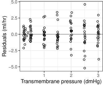
Figure 1: Plot of the conditional residuals against the transmembrane pressure for model dialyzer_mod.

To check if this pattern is actually indicative of a problem, we can construct a lineup of residual plots. To do this, we must generate data from a number, say 19, properly specified models to serve as decoy residual plots. Then, we create a faceted set of residual plots where the observed residual plot (Figure 1) is randomly assigned to a facet. To generate the residuals from properly specified models, we use bootstrap() to run a parametric bootstrap, and use hlm_resid() from HLMdiag (Loy and Hofmann, 2014) to extract a data frame containing the residuals from each bootstrap sample:

set.seed(1234)library(HLMdiag)sim_resids <- bootstrap(dialyzer_mod, .f = hlm_resid, type = "parametric", B = 19)

The simulated residuals are stored in the replicates element of the sim_resids list. sim_resids$replicates is a tibble containing the 19 bootstrap samples, with the the replicate number stored in the .n column.

dplyr::glimpse(sim_resids$replicates)

#> Rows: 2,660#> Columns: 15#> $ id              <dbl> 1, 2, 3, 4, 5, 6, 7, 8, 9, 10, 11, 12, 13, 14, 15, 16,~#> $ rate            <dbl> -0.8579225, 17.0489071, 34.3658850, 44.8495706, 44.525~#> $ pressure        <dbl> 0.240, 0.505, 0.995, 1.485, 2.020, 2.495, 2.970, 0.240~#> $ `I(pressure^2)` <I<dbl>>   0.0576, 0.255025, 0.990025, 2.205225,   4.0804, 6~#> $ `I(pressure^3)` <I<dbl>>     0.013824,  0.128787625,  0.985074875,  3.274759~#> $ `I(pressure^4)` <I<dbl>>   0.00331776, 0.065037...., 0.980149...., 4.863017.~#> $ QB              <fct> 200, 200, 200, 200, 200, 200, 200, 200, 200, 200, 200,~#> $ Subject         <ord> 1, 1, 1, 1, 1, 1, 1, 2, 2, 2, 2, 2, 2, 2, 3, 3, 3, 3, ~#> $ .resid          <dbl> -1.19760128, 0.65599523, -0.90104281, 1.39131416, 0.11~#> $ .fitted         <dbl> 0.3396788, 16.3929119, 35.2669278, 43.4582564, 44.4101~#> $ .ls.resid       <dbl> -0.51757742, 1.23968773, -1.32231148, 0.59071027, 0.30~#> $ .ls.fitted      <dbl> -0.3403451, 15.8092194, 35.6881965, 44.2588603, 44.223~#> $ .mar.resid      <dbl> -2.1236411, -0.3100340, -2.1298265, -0.3453041, -2.455~#> $ .mar.fitted     <dbl> 1.265719, 17.358941, 36.495712, 45.194875, 46.981067, ~#> $ .n              <int> 1, 1, 1, 1, 1, 1, 1, 1, 1, 1, 1, 1, 1, 1, 1, 1, 1, 1, ~

Now, we can use the lineup() function from nullabor (Buja et al., 2009) to generate the lineup data. lineup() will randomly insert the observed (true) data into the samples data, “encrypt” the position of the observed data, and print a message that you can later decrypt in the console.

library(nullabor)lineup_data <- lineup(true = hlm_resid(dialyzer_mod), n = 19, samples = sim_resids$replicates)

#> decrypt("EnXL zNTN Z6 PJfZTZJ6 Wy")

dplyr::glimpse(lineup_data)

#> Rows: 2,800#> Columns: 15#> $ id              <dbl> 1, 2, 3, 4, 5, 6, 7, 8, 9, 10, 11, 12, 13, 14, 15, 16,~#> $ rate            <dbl> -0.8579225, 17.0489071, 34.3658850, 44.8495706, 44.525~#> $ pressure        <dbl> 0.240, 0.505, 0.995, 1.485, 2.020, 2.495, 2.970, 0.240~#> $ `I(pressure^2)` <I<dbl>>   0.0576, 0.255025, 0.990025, 2.205225,   4.0804, 6~#> $ `I(pressure^3)` <I<dbl>>     0.013824,  0.128787625,  0.985074875,  3.274759~#> $ `I(pressure^4)` <I<dbl>>   0.00331776, 0.065037...., 0.980149...., 4.863017.~#> $ QB              <fct> 200, 200, 200, 200, 200, 200, 200, 200, 200, 200, 200,~#> $ Subject         <ord> 1, 1, 1, 1, 1, 1, 1, 2, 2, 2, 2, 2, 2, 2, 3, 3, 3, 3, ~#> $ .resid          <dbl> -1.19760128, 0.65599523, -0.90104281, 1.39131416, 0.11~#> $ .fitted         <dbl> 0.3396788, 16.3929119, 35.2669278, 43.4582564, 44.4101~#> $ .ls.resid       <dbl> -0.51757742, 1.23968773, -1.32231148, 0.59071027, 0.30~#> $ .ls.fitted      <dbl> -0.3403451, 15.8092194, 35.6881965, 44.2588603, 44.223~#> $ .mar.resid      <dbl> -2.1236411, -0.3100340, -2.1298265, -0.3453041, -2.455~#> $ .mar.fitted     <dbl> 1.265719, 17.358941, 36.495712, 45.194875, 46.981067, ~#> $ .sample         <dbl> 1, 1, 1, 1, 1, 1, 1, 1, 1, 1, 1, 1, 1, 1, 1, 1, 1, 1, ~

With the lineup data in hand, we can create a lineup of residual plots using facet_wrap():

ggplot(lineup_data, aes(x = pressure, y = .resid)) +  geom_hline(yintercept = 0, color = "gray60") +  geom_point(shape = 1) +  facet_wrap(~.sample) +  theme_bw() +  labs(x = "Transmembrane pressure (dmHg)", y = "Residuals (ml/hr)")

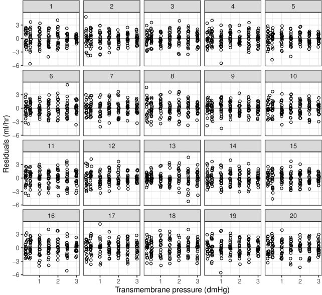
Figure 2: A lineup of the conditional residuals against the transmembrane pressure for model dialyzer_mod. One of the facets contains the true residual plot generated from the fitted model, the others are decoys generated using a parametric bootstrap.

In Figure 2, the observed residual plot is in position 13. If you can discern this plot from the field of decoys, then there is evidence that the fitted homogeneous LME model is deficient. In this case, we believe 13 is discernibly different, as expected based on the discussion in Pinheiro and Bates (2000). We refer the reader to Loy et al. (2017) for a discussion of additional diagnostic lineup plots.

User-specified statistics: Estimating repeatibility

The beauty of the bootstrap is its flexibility. Interval estimates can be constructed for functions of model parameters that would otherwise require more complex derivations. For example, the bootstrap can be used to estimate the intraclass correlation. The intraclass correlation mesaures the proportion of the total variance in the response accounted for by groups, and is an important measure of repeatability in ecology and evolutionary biology (Nakagawa and Schielzeth, 2010). As a simple example, we’ll consider the BeetlesBody data set in rptR (Stoffel et al., 2017). This simulated data set contains information on body length (BodyL) and the Population from which the beetles were sampled. A simple Guassian-response LME model of the form

$$y_{ij}=\beta_{0}+b_{i}+\varepsilon_{ij},\qquad b_{i}\sim\mathcal{N}(0,\sigma^{2}_{b}),\qquad\varepsilon_{ij}\sim\mathcal{N}(0,\sigma^{2}),$$

can be used to describe the body length of beetle $j$ from population $i$. The repeatability is then calculated as $R=\sigma^{2}_{b}/(\sigma^{2}_{b}+\sigma^{2})$. Below we fit this model using lmer():

data("BeetlesBody", package = "rptR")(beetle_mod <- lmer(BodyL ~ (1 | Population), data = BeetlesBody))

#> Linear mixed model fit by REML [’lmerMod’]#> Formula: BodyL ~ (1 | Population)#>    Data: BeetlesBody#> REML criterion at convergence: 3893.268#> Random effects:#>  Groups     Name        Std.Dev.#>  Population (Intercept) 1.173#>  Residual               1.798#> Number of obs: 960, groups:  Population, 12#> Fixed Effects:#> (Intercept)#>       14.08

To construct a bootstrap confidence interval for the repeatability, we first must write a function to calculate it from the fitted model. Below we write a one-off function for this model to demonstrate a “typical” workflow rather than trying to be overly general.

repeatability <- function(object) {  vc <- as.data.frame(VarCorr(object))  vc$vcov[1] / (sum(vc$vcov))}

The original estimate of repeatability can then be quickly calculated:

repeatability(beetle_mod)

#> [1] 0.2985548

To construct a bootstrap confidence interval of repeatability, we run the desired bootstrap procedure, specifying .f = repeatability and then pass the results to confint().

(beetle_boot <- bootstrap(beetle_mod, .f = repeatability, type = "parametric", B = 2000))

#> Bootstrap type: parametric#>#> Number of resamples: 2000#>#>    observed  rep.mean         se        bias#> 1 0.2985548 0.2845316 0.08997414 -0.01402321#>#> There were 0 messages, 0 warnings, and 0 errors.#>#> The most commonly occurring message was: NULL#>#> The most commonly occurring warning was: NULL#>#> The most commonly occurring error was: NULL

(beetle_ci <- confint(beetle_boot, type = "basic"))

#> # A tibble: 1 x 6#>   term  estimate lower upper type  level#>   <chr>    <dbl> <dbl> <dbl> <chr> <dbl>#> 1 ""       0.299 0.136 0.480 basic  0.95

Notice that the term column of beetle_ci is an empty character string since we did not have repeatability return a named vector.

Alternatively, we can plot() the results, as shown in Figure 3. The plot method for lmeresamp objects uses stat_halfeye() from ggdist (Kay, 2021) to render a density plot with associated 66% and 95% percentile intervals.

plot(beetle_boot, .width = c(.5, .9)) +  labs(    title = "Bootstrap repeatabilities",    y = "density",    x = "repeatability"  )

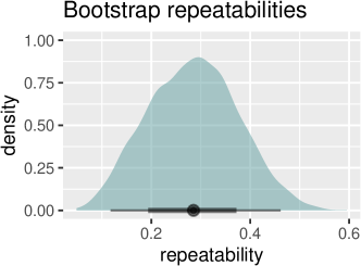
Figure 3: Density plot with 66% and 95% percentile intervals of the bootstrap repeatibilities.

Bootstrapping in parallel

Bootstrapping is a computationally demanding task, but bootstrap iterations do not rely on each other, so they are easy to implement in parallel. Rather than building parallel processing into lmeresampler, we have created a utility function, combine_lmeresamp(), that allows the user to easily implement parallel processing using doParallel (Microsoft and Weston, 2020) and foreach (Microsoft and Weston, 2020). The code is thus concise and simple enough for users without much experience with parallelization, while also providing flexibility to the user.

doParallel and foreach default to multicore (i.e., forking) functionality when using parallel computing on UNIX operating systems and snow-like (i.e., clustering) functionality on Windows systems. In this section, we will use clustering in our example. For more information on forking, we refer the reader to the vignette in Microsoft and Weston (2020).

The basic idea behind clustering is to execute tasks as a “cluster” of computers. Each cluster needs to be fed in information separately, and as a consequence clustering has more overhead than forking. Clusters also need to be made and stopped with each call to foreach() to explicitly tell the CPU when to begin and end the parallelization.

Below, we revisit the JSP example and distribute 2000 bootstrap iterations equally over two cores:

library(foreach)library(doParallel)set.seed(5678)# Starting a cluster with 2 coresno_cores <- 2cl <- makeCluster(no_cores)registerDoParallel(cores = no_cores)# Run 1000 bootstrap iterations on each coreboot_parallel <- foreach(  B = rep(1000, 2),  .combine = combine_lmeresamp,  .packages = c("lmeresampler", "lme4")) %dopar% {  bootstrap(jsp_mod, .f = fixef, type = "parametric", B = B)}# Stop the clusterstopCluster(cl)

The combine_lmeresamp() function combines the two lmeresamp objects that are returned from the two bootstrap() calls into a single lmeresamp object. Consequently, working with the returned object proceeds as previously discussed.

It’s important to note that running a process on two cores does not yield a runtime that is twice as fast as running the same process on one core. This is because parallelization takes some overhead to split the processes, so while runtime will substantially improve, it will not correspond exactly to the number of cores being used. For example, the runtime for the JSP example run on a single core was

#>    user  system elapsed#>  38.213   0.368  38.800

and the runtime for the JSP run on two cores was

#>    user  system elapsed#>   0.037   0.029  19.324

These timings were generated using system.time() on a MacBook Pro with a 2.9 GHz Quad-Core Intel Core i7 processor. In this set up, running the 2000 bootstrap iterations over two cores reduced the runtime by a factor of about 2.01, but this will vary for each user.

Summary

In this paper, we discussed our implementation of five bootstrap procedures for nested, Gaussian LME models fit via the nlme or lme4 packages. The bootstrap() function in lmeresampler provides a unified interface to these procedures, allowing users to easily bootstrap their fitted LME models. In our examples, we illustrated the basic usage of the bootstrap, how it can be used to create simulation-based visual diagnostics, and how to it can be used to estimate functions of parameters from the LME model. The bootstrap approach to inference is computationally intensive, so we have also demonstrated how users can bootstrap in parallel.

While this paper focused solely on the nested, Gaussian-response LME model, lmeresampler implements bootstrap procedures for a wide class of models. Specifically, the cases, residual, and parametric bootstraps can be used to bootstrap generalized LME models fit via lme4::glmer(). Additionally, the parametric bootstrap works with LME models with crossed random effects, though the results may not be optimal (Mccullagh, 2000). Future development of lmeresampler will focus on implementing additional extensions, especially for crossed data structures.

Adam Loy
Department of Mathematics and Statistics
Carleton College
Northfield, MN United States of America
https://aloy.rbind.io/
ORCiD: 0000-0002-5780-4611
aloy@carleton.edu

Jenna Korobova
Department of Mathematics and Statistics
Carleton College
Northfield, MN, United States of America

jenna.korobova@gmail.com,

References

- Bates et al. (2015) D. Bates, M. Mächler, B. Bolker, and S. Walker. Fitting linear mixed-effects models using lme4. Journal of Statistical Software, 67(1):1–48, 2015. URL https://doi.org/10.18637/jss.v067.i01.
- Buja et al. (2009) A. Buja, D. Cook, H. Hofmann, M. Lawrence, E. kyung Lee, D. F. Swayne, and H. Wickham. Statistical inference for exploratory data analysis and model diagnostics. Royal Society Philosophical Transactions A, 367(1906):4361–4383, 2009. URL https://doi.org/10.1098/rsta.2009.0120.
- Carpenter et al. (2003) J. R. Carpenter, H. Goldstein, and J. Rasbash. A novel bootstrap procedure for assessing the relationship between class size and achievement. Journal of the Royal Statistical Society, Series C, 52(4):431–443, 2003. URL https://doi.org/10.1111/1467-9876.00415.
- Chambers and Chandra (2013) R. Chambers and H. Chandra. A random effect block bootstrap for clustered data. Journal of Computational and Graphical Statistics, 22(2):452–470, 2013. URL https://doi.org/10.1080/10618600.2012.681216.
- Davidson and Flachaire (2008) R. Davidson and E. Flachaire. The wild bootstrap, tamed at last. Journal of econometrics, 146(1):162–169, 2008. URL https://doi.org/10.1016/j.jeconom.2008.08.003.
- Field and Welsh (2007) C. A. Field and A. H. Welsh. Bootstrapping clustered data. Journal of the Royal Statistical Society, Series B, 69(3):369–390, 2007. URL https://doi.org/10.1111/j.1467-9868.2007.00593.x.
- Flachaire (2005) E. Flachaire. Bootstrapping heteroskedastic regression models: wild bootstrap vs. pairs bootstrap. Computational statistics & data analysis, 49(2):361–376, 2005. URL https://doi.org/10.1016/j.csda.2004.05.018.
- Galecki and Burzykowski (2013) A. Galecki and T. Burzykowski. Linear Mixed-Effects Models Using R: A Step-by-Step Approach. Springer, New York, 2013. URL https://doi.org/10.1007/978-1-4614-3900-4.
- Goldstein (2011) H. Goldstein. Multilevel Statistical Models. John Wiley & Sons, Ltd., West Sussex, 4 edition, 2011. URL https://doi.org/10.1002/9780470973394.
- Halekoh and Højsgaard (2014) U. Halekoh and S. Højsgaard. A kenward-roger approximation and parametric bootstrap methods for tests in linear mixed models – the R package pbkrtest. Journal of Statistical Software, 59(9):1–30, 2014. URL https://doi.org/10.18637/jss.v059.i09.
- Haslett and Haslett (2007) J. Haslett and S. J. Haslett. The three basic types of residuals for a linear model. International statistical review, 75(1):1–24, 2007. URL https://doi.org/10.1111/j.1751-5823.2006.00001.x.
- Kay (2021) M. Kay. ggdist: Visualizations of Distributions and Uncertainty, 2021. URL https://doi.org/10.5281/zenodo.3879620. R package version 2.4.0.
- Liu (1988) R. Y. Liu. Bootstrap procedures under some non-i.i.d. models. Annals of statistics, 16(4):1696–1708, Dec. 1988. URL https://doi.org/10.1214/aos/1176351062.
- Loy and Hofmann (2014) A. Loy and H. Hofmann. HLMdiag: A suite of diagnostics for hierarchical linear models in R. Journal of Statistical Software, 56(5):1–28, 2014. URL https://doi.org/10.18637/jss.v056.i05.
- Loy et al. (2017) A. Loy, H. Hofmann, and D. Cook. Model choice and diagnostics for linear Mixed-Effects models using statistics on street corners. Journal of Computational and Graphical Statistics, 26(3):478–492, 2017. URL https://doi.org/10.1080/10618600.2017.1330207.
- Mammen (1993) E. Mammen. Bootstrap and wild bootstrap for high dimensional linear models. Annals of statistics, 21(1):255–285, 1993. URL https://doi.org/10.1214/aos/1176349025.
- Mccullagh (2000) P. Mccullagh. Resampling and exchangeable arrays. Bernoulli, 6(2):285–301, 2000. URL https://doi.org/10.2307/3318577.
- Microsoft and Weston (2020) Microsoft and S. Weston. doParallel: Foreach Parallel Adaptor for the ’parallel’ Package, 2020. URL https://CRAN.R-project.org/package=doParallel. R package version 1.0.16.
- Microsoft and Weston (2020) Microsoft and S. Weston. foreach: Provides Foreach Looping Construct, 2020. URL https://CRAN.R-project.org/package=foreach. R package version 1.5.1.