THE X-RAYS WIND CONNECTION IN PG 2112+059

Abstract

We study the connection between the X-ray and UV properties of the broad absorption line (BAL) wind in the highly X-ray variable quasar PG 2112+059 by comparing Chandra-ACIS data with contemporaneous UV HST/STIS spectra in three different epochs. We observe a correlation whereby an increase in the equivalent-widths (EWs) of the BALs is accompanied by a redder UV spectrum. The growth in the BALs EWs is also accompanied by a significant dimming in soft X-ray emission ($\lesssim 2\,\text{keV}$), consistent with increased absorption. Variations in the hard X-ray emission ($\gtrsim 2\,\text{keV}$) are only accompanied by minor spectral variations of the UV-BALs and do not show significant changes in the EW of BALs. These trends suggest a wind-shield scenario where the outflow inclination with respect to the line of sight is decreasing and/or the wind mass is increasing. These changes elevate the covering fraction and/or column densities of the BALs and are likely accompanied by a nearly contemporaneous increase in the column density of the shield.

1 Introduction

It is well established that, with exception of dwarf galaxies, every galaxy should have a supermassive black hole (SMBH) with black hole masses ($M_{\rm BH}$) of $10^{6}M_{\odot}\lesssim M_{\rm BH}\lesssim 10^{10}M_{\odot}$ in their centers (e.g., Mezcua et al., 2018; Kormendy & Ho, 2013). Active Galactic Nuclei (AGN), which in their brightest states become quasars, in brief (of the order of $10^{7}$ years; Haehnelt & Rees, 1993) and powerful duty cycles are thought to regulate SMBH growth (Soltan, 1982). AGN should also transport energy from the SMBH to their surrounding host galaxy (e.g, Fabian, 2012) through various feedback mechanisms, including jets and quasar winds (or accretion disk winds). These two mechanisms are key ingredients to explain the regulation of galaxy evolution, and the origin of known observational relationships between the SMBH masses and bulge properties in nearby galaxies (e.g., Hopkins et al., 2006; Somerville et al., 2008; Kormendy & Ho, 2013).

Evidence of winds is observed in the ultra-violet (UV) rest-frame spectra in a fraction of quasars ($\sim 20\%$, e.g., Hewett & Foltz, 2003; Gibson et al., 2009) through ionized broad absorption lines (BALs). These spectral features with broadening above $2000$ km s^-1 (Weymann et al., 1991) appear as absorption with blueshifted velocity offsets of $2,000$ to $30,000$ km s^-1 from the line rest-frame. Depending on the ionization state of the wind, BAL quasars are divided into at least two categories (e.g. Hall et al., 2002): high-ionization BAL quasars (HiBALs) and low-ionization BAL quasars (LoBALs). HiBALs show absorption features from O vi, N v, and C iv lines. LoBALs are characterized to have high-ionization absorption plus absorption from Al iii, C ii  and/or Mg ii lines.

Observations and theory suggest that quasar BAL features are an orientation effect (e.g., Murray et al., 1995; Risaliti & Elvis, 2010; Filiz Ak et al., 2014), and thus these outflows should be intrinsic to every quasar. Models predict that BALs originate from the accretion disk in funnel shaped structures at distances of $10^{2}-10^{3}R_{S}$ (where $R_{S}=2GM_{\rm BH}/c^{2}$ is the Schwarzschild radius) from their central SMBH (e.g., Murray et al., 1995; Proga et al., 2000). In contrast, larger distances of $10^{3}-10^{7}R_{S}$ are inferred from the BAL observational signatures (e.g., de Kool et al., 2001; Hall et al., 2011; Arav et al., 2013). Similar distance estimates are found for narrow absorption lines (NAL) and mini-BALs quasars (e.g., Misawa et al., 2016; Xu et al., 2019). Therefore, UV outflows could be observed far from their origin or a revision on their models is needed. BAL quasars also tend to show particularly distinctive weak X-ray emission (e.g., Gibson et al., 2009), which has been attributed to absorption (e.g., Page et al., 2017) and/or intrinsically weak emission (e.g., Luo et al., 2014).

The growing evidence from BAL quasar spectral features from UV to X-rays has motivated many models. These models postulate that outflows are launched in funnel shaped structures driven by radiation and/or magnetic forces from the accretion disk (e.g., Murray et al., 1995; Proga et al., 2000; Fukumura et al., 2010). In view of these models, BALs correspond to lines of sight that are intercepting these structures. Additionally, the weak X-ray emission could be a product of absorption from the inner parts $\lesssim 100\,R_{S}$ of the medium that is not accelerated enough to be expelled to the inter galactic medium (IGM; failed wind). There could be also a highly ionized part of the wind accelerated to relativistic speeds $\gtrsim 0.1c$ (with $c$ the speed of light) and showing spectral signatures in the X-ray through highly ionized Fe xxv and Fe xxvi BAL lines (e.g., Chartas et al., 2002, 2003; Saez & Chartas, 2011; Hamann et al., 2018).

The HiBAL quasar PG 2112+059  with $z=0.459$ (Monroe et al., 2016) and $M_{V}=-27.3$ is one of the most luminous PG quasars. It has been observed in X-rays from 1991-2007 by various X-ray missions, including ROSAT, ASCA, XMM-Newton, and Chandra. In these observations, PG 2112+059 has shown typical BAL X-ray weakness and order of magnitude X-ray flux changes over periods of time as short as 6 months (Saez et al., 2012). The physical model that leads to the observed X-ray emission is not well understood. It could be a reflection-type model (e.g., Schartel et al., 2010) or a complex absorption model (e.g., Gallagher et al., 2004; Saez et al., 2012). In this work, our main goal is to analyze the connection between the strong X-ray variability of PG 2112+059 and the physical properties that the associated BAL winds present in the UV. Through this kind of joint analysis, we are aiming to better understand the mechanisms that create these winds. Throughout this paper, unless stated otherwise, we use cgs units, errors are quoted at the 1$\sigma$ level, and we adopt a flat $\Lambda$-dominated universe with $H_{0}=70~{}\hbox{km~{}s${}^{-1}$}\;{\rm Mpc^{-1}}$, $\Omega_{\Lambda}=0.7$, and $\Omega_{M}=0.3$.

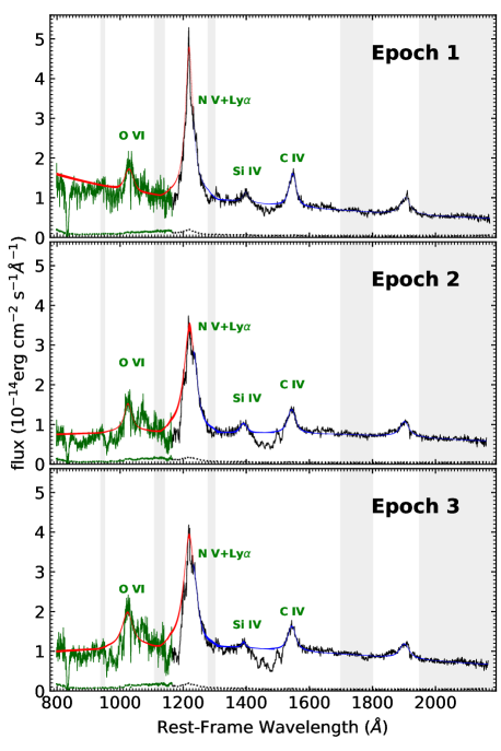
Figure 1: HST UV spectra of PG 2112+059 illustrating the presence of O vi, N v, and C iv BALs. The upper, middle and lower panel correspond to epochs 1, 2 and 3, respectively. The green and black curves indicate the G140L and G230L grating spectra, while, the red and blue curves are the fitted spectral model in the extreme-UV and far-UV (EUV and FUV) wavelength bands (see §2.3) with thickness given by the 1$\sigma$ confidence region and the dotted line is the spectral error. The gray areas are the wavelength ranges where continua fits are performed.

2 METHODOLOGY

2.1 Observations

Table 1: Log of Chandra observations of PG 2112+059

		exp. time		rate
obs. date	obs. id	(ks)	counts	(10-3 s-1)	Ref.a
2002/09/01 (Epoch 1)	3011	56.9	$829_{-29}^{+30}$	14.6$\pm$0.5	1
2014/12/20 (Epoch 2)	17553	18.2	$62_{-8}^{+9}$	3.4$\pm$0.5	2
2015/08/29 (Epoch 3)	17148	18.3	$140_{-12}^{+13}$	7.6$\pm$0.7	2

All observations utilize the ACIS-S3 detector. The counts and rates are from background-subtracted source photon counts in the Chandra full-band (0.5–8 keV). The exposure times, photon counts, and rates are obtained after screening the data. The errors on the source counts were computed by propagating the asymmetric errors on the total and background counts using the approach of Barlow (2004). The total and background count errors were estimated from Tables 1 and 2 of Gehrels (1986).

^a References: (1) Gallagher et al. (2004); (2) This work.

Table 2: Log of HST STIS observations of PG 2112+059

		exp. time
obs. date	prop. id	(s)	instrument	grating	wave-range	ra	Ref.b
2002/09/01 (Epoch 1)	9277	1100	FUV-MAMA	G140L	1150$-$1730	1223	1
2002/09/01 (Epoch 1)	9277	900	NUV-MAMA	G230L	1570$-$3180	767	1
2014/12/18 (Epoch 2)	13948	1095	FUV-MAMA	G140L	1150$-$1730	1222	2
2014/12/18 (Epoch 2)	13948	920	NUV-MAMA	G230L	1570$-$3180	767	2
2015/09/11 (Epoch 3)	13948	1095	FUV-MAMA	G140L	1150$-$1730	1222	2
2015/09/11 (Epoch 3)	13948	920	NUV-MAMA	G230L	1570$-$3180	767	2

The STIS observations utilize the following gratings: G140L for the FUV-MAMA and G230L for the NUV-MAMA configurations.

^a The spectral resolution ($R=\lambda/\Delta\lambda$) is calculated at the central wavelength of each configuration, i.e. at 1425 Å and 2376 Å for the FUV-MAMA and NUV-MAMA configurations, respectively.

^b References: (1) Gallagher et al. (2004); (2) This work.

In this work, we analyze two $\sim 20$ ks Chandra observations each with a contemporaneous HST STIS spectrum, performed in 2014–2015 and separated by approximately nine months. These new observations are compared with a nearly simultaneous archival Chandra-HST observation from 2002 (analyzed in Gallagher et al., 2004). Each Chandra observation was performed within $\sim$10 days of an HST observation. During the Chandra-HST time gap although there could be X-ray spectral variability, this should not be important when compared to long term ($\gtrsim 6$ months) spectral variability. Based on the existing constraints for PG 2112+059 we expect that any significant X-ray spectral variability (relevant for this study) should be on time scales $\gtrsim 1$ month. For instance, in the period between May 3 and November 5 of 2007 PG 2112+059 has 4 XMM-Newton observations each with at least 500 0.3–10 keV counts (see Saez et al., 2012, for details). During this period, no significant variability was detected (at a 99% level), such that any potential flux variations were less than 20%. Additionally, on time scales $\lesssim 1$ month, it is expected that fractional changes in the normalized continuum flux removed by absorption should be $\lesssim 10$% in the UV BALs (e.g., Capellupo et al., 2013). On time scales longer than a month the fraction of the normalized flux removed by absorption could change more dramatically in BALs. As we do not expect strong variability either in the X-ray flux or in the UV BALs absorption profiles in scales $\lesssim 1$ month, hereafter, we will refer to each contemporaneous Chandra-HST observation time-ordered epoch as 1, 2 or 3. Details about the dates and most important characteristics of these three sets of Chandra-HST spectra can be found in Table 1 for the Chandra observations and in Table 2 for the HST observations.

The Chandra observations were reduced using the standard software CIAO version 4.12 provided by the Chandra X-ray Center (CXC). For each epoch, we reprocessed the datasets through the chandra_repro script to obtain the latest calibration. Source and background spectra and associated products were extracted using the CIAO script specextract from a circular region with an aperture radius of 4″ and an annular source-free region with an inner radius of 6″ and an outer radius of 24″, respectively. The numbers of background-subtracted counts in the source regions at energies of 0.5–8 keV and some details about the Chandra observations are presented in Table 1.

The HST spectra were reduced with the standard STIS pipeline, and the resulting spectra are expected to have a flux calibration at the $\sim 5$% level of precision (Bostroem & Proffitt, 2011). The HST STIS spectra span a wavelength range of 1570–3180 Å which in the rest frame of PG 2112+059 sample several important BAL features such as O vi, Ly$\alpha$, N v, Si iv, and C iv. In each HST observation epoch, the exposure was $\sim 1100$ s and $\sim 900$ s for the G140L and G230L gratings, respectively, (see Table 2) both with a $52\arcsec\times 0\aas@@fstack{\prime\prime}2$ slit. The spectra have dispersions on average of $\approx 0.58$ Å and $\approx 1.54$ Å per pixel for the G140L and G230L gratings, and resolving powers of $R\approx 1220$ and $R\approx 770$ at the grating central wavelengths of 1425 Å and 2376 Å, respectively. The G140L and G230L grating spectra overlap in the range 1570–1730 Å. In this wavelength overlap region, as a product of the calibration, each grating spectra show decreasing signal-to-noise ratios (S/N) per pixel at their respective endpoints. Therefore, for our analysis, we select a limiting wavelength of 1700 Å ($\approx 1170$ Å in the rest-frame of PG 2112+059) as the end of the G140L spectrum and beginning of the G230L spectrum. This wavelength is approximately where both gratings reach the same S/N in wavelength bins of comparable sizes. In each observation, the S/N in the continuum is on average $\approx 10$ (19) per pixel with a standard deviation of $\approx 3$ (5) for the G140L (G230L) grating. The full reduced and dereddened HST spectrum of PG 2112+059 at each epoch is presented in Figure 1. The dereddening has been obtained by assuming a Galactic extinction of $E(B-V)=0.0904$ (from Schlegel et al., 1998), equivalent to $N_{H}\approx 6\times 10^{20}\,$cm^-2 (e.g., Güver & Özel, 2009), where $N_{\rm H}$ is the total (neutral an ionized) hydrogen column density. The reddening model used here and hereafter is that of Pei (1992).

Table 3: Chandra X-ray  spectral fits statistics

	$C$-statistic/dof
epoch	APL	WADR	$p$-values
1	504.0/509	459.7/508	0.000
2	235.8/509	231.1/508	0.007
3	374.9/509	365.7/508	0.002

Table 4: Chandra X-ray  spectral fits parameters of the WAPLR model

epoch	${N}_{\rm H}$	log $\xi$	normPL	normR
(1)	(2)	(3)	(4)	(5)
1	12$\pm$ 2	2.14$\pm$0.03	6.4$\pm$1.0	14.6$\pm$5.5
2	64$\pm$ 42	3.02$\pm$1.49	1.4$\pm$0.3	13.9$\pm$7.7
3	16$\pm$ 2	1.95$\pm$0.03	7.5$\pm$1.4	1.6$\pm$5.3

Col. (1): Observation Epoch. Col. (2): Column density in units of $10^{22}$ cm^-2. Col. (3): Logarithm of the ionization parameter $\xi=L/n\,r^{2}$, as defined in xspec. Col. (4–5): Normalizations of the continuum power-law and the reflection model (pexmon). Both normalizations are in units of $10^{-5}\,{\rm counts\>\,cm^{-2}\,s^{-1}\,keV^{-1}}$.

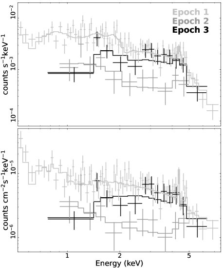
Figure 2: Folded (upper panel) and unfolded (lower panel) Chandra spectra of PG 2112+059. The solid histograms indicate the best-fitting WAPLR model to each observation. The light gray, gray, and black colors are associated with epochs 1, 2 and 3, respectively. In each observation a grouping with a minimum 10 counts per bin has been used.

2.2 X-ray analysis

Given that both of our new Chandra observations of PG 2112+059 have very modest count statistics, we performed fits in the 0.5–8 keV band using the $C$-statistic (Cash, 1979) in xspec (Arnaud, 1996). Additionally, in all the X-ray models used here Galactic absorption with total hydrogen column density of $\hbox{${N}_{\rm H}$}=6.0\times 10^{20}$ cm^-2 is assumed (Kalberla et al., 2005). We use unbinned data and thus the $C$-statistic may not be appropriate to utilize when performing background subtraction. For this purpose, we fit the background spectra with a flat response using the cplinear model (Broos et al., 2010). The background model is scaled and subtracted when we fit the source spectra. Our new X-ray observations were designed to provide flux constraints, and with this goal we use a model that is simple and at the same time provides good fits to our observations.

To fit the Chandra spectra, we select a model used in Schartel et al. (2010) consisting of a continuum power law and an ionized reflection component, these both pass through a warm absorber. Hereafter we will refer to this model as the warm-absorbed power-law and reflection model (WAPLR; xspec model phabs*zxipcf*(pow+pexmon)). To avoid overfitting our spectra we fixed many of the parameters that describe the WAPLR model, leaving 4 degrees of freedom: the normalization of the continuum power-law (${\rm norm_{PL}}$), the normalization of the reflection component (${\rm norm_{R}}$), and the column density (${N}_{\rm H}$) and the logarithm of ionization parameter (as defined by xspec; $\log\xi$) of the warm absorber.

The selection of the WAPLR model over a simpler model like the absorbed power-law model (APL; xspec model phabs*zphabs*pow) is based on evidence of spectral complexity that includes the presence of a reflection component in previous PG 2112+059 high S/N spectra (e.g., Schartel et al., 2010; Saez et al., 2012). Additionally, the WAPLR model is a good representation of the data in past XMM-Newton observations of PG 2112+059 (Schartel et al., 2007, 2010), and provides significant improvements over the fits of an APL model over Epochs 1–3 (see next paragraph). In Figure 2 we present the Chandra spectra with their respective WAPLR fits. As this figure shows, the WAPLR model reproduces the significant Fe K$\alpha$ emission feature at rest-frame energies $\sim 6.4~{}{\rm keV}$ (feature at $\sim 4.4$ keV in Figure 2) found in Epoch 1 (Gallagher et al., 2004).

In Epochs 1–3 we check that the WAPLR model shows an improvement in the fits (lower values of $C$-statistic; see Table 3) when compared with the APL model. We test these fit improvements by using a modified version of the likelihood ratio test (LRT) routine provided by the xspec package. Using this routine we generate 1000 Monte Carlo simulated spectra from the fits of the APL model. These simulated spectra are fitted with both the APL and WAPLR models to generate a table of $\Delta C$, where $\Delta C$ is the difference between values of the $C$-statistic obtained with the APL and the WAPLR model. The $p$-values correspond to the fraction of fits where $\Delta C>\Delta C_{\rm obs}$, where $\Delta C_{\rm obs}$ is the observed value of $\Delta C$. From the simulated data, in Epochs 1 and 3 we check that the WAPLR provides a significant improvement over the fit with the APL model ($p\lesssim 0.002$) (see Table 3). We also find in Epoch 2 a significant improvement on the fits (with $p\approx 0.007$), albeit, this observation might not have enough counts to be reliable in differentiating between model fits. The best-fitted parameters and fluxes obtained from the WAPLR model are presented in Tables 4 and 5. Hereafter (if not stated otherwise), we assume that any X-ray parameter estimated from spectral fits is obtained from WAPLR model using the $C$-statistic.

Table 5: X-ray fluxes and Luminosities of PG 2112+059

epoch	$f_{0.5-2}$	$f_{2-8}$	$f_{0.5-8}$	$f_{\rm 2keV}$	$\Gamma_{\rm eff}$	HR	${\rm log}\,L_{\rm 2keV}$	log $L_{2-10}$
(1)	(2)	(3)	(4)	(5)	(6)	(7)	(8)	(9)
1	3.2$\pm$0.2	16$\pm$ 1	19$\pm$ 1	5.5$\pm$0.4	0.85$\pm$0.08	0.21$\pm$0.04	25.47$\pm$0.03	44.07$\pm$0.03
2	1.1$\pm$0.5	4$\pm$ 2	5$\pm$ 3	1.5$\pm$0.7	1.00$\pm$0.61	0.15$\pm$0.14	24.90$\pm$0.21	43.48$\pm$0.17
3	1.2$\pm$0.2	13$\pm$ 2	14$\pm$ 2	2.5$\pm$0.3	0.29$\pm$0.14	0.43$\pm$0.08	25.12$\pm$0.06	43.96$\pm$0.06

X-ray fluxes, luminosities and total hydrogen column densities are corrected for Galactic absorption assuming $\hbox{${N}_{\rm H}$}=6.0\times 10^{20}$ cm^-2  (Kalberla et al., 2005) and are obtained from the best-fitting parameters for a WAPLR model (xspec model phabs*zxipcf*[pow+pexmon]). Col. (1): Observation Epoch. Cols. (2–4): Observed fluxes in the 0.5–2 keV, 2–8 keV, and 0.5–8 keV  bands in units of $10^{-14}$ erg cm^-2 s^-1. Col. (5): Observed flux densities at rest-frame  2 keV in units of $10^{-32}$ erg cm^-2 s^-1Hz^-1. Col. (6): X-ray effective photon index $\Gamma_{\rm eff}=-\alpha_{x}+1$ obtained from the ratio of of 2–8 keV to 0.5–2 keV flux assuming power-law spectra ($f_{\nu}\propto\nu^{\alpha_{x}}$). Col. (7): Hardness ratio, corrected due to time-dependent loss of Chandra-ACIS sensitivity (see §3 for details). Col. (8) Logarithm of the monochromatic luminosity at rest-frame 2 keV. Col. (9) Logarithm of the luminosity at rest-frame 2–10 keV.

2.3 UV Continuum Fit and Normalization

To describe the C iv BAL, we fit the HST/UV continuum in three relatively line-free (RLF) windows at rest-frame wavelengths in the far-UV band (FUV; $>1200$ Å) of PG 2112+059: 1280–1300 Å, 1700–1800 Å, and 1950–2200 Å. These RLF windows were selected in a similar fashion as Gibson et al. (2009), with a small difference in the first RLF window. For this window, the lower wavelength limit is 1280Å (instead 1250Å) in order to avoid the broad Ly$\alpha$+N v emission line. Additionally, the upper limit is 1300Å (instead 1350Å) in order to avoid a possible BAL Si iv region. The continuum in the extreme-UV (EUV) band ($<1200$ Å) is expected to have thermal signatures of the accretion disk (i.e., big-blue-bump features; e.g. Telfer et al., 2002; Zheng et al., 1997) and to exhibit significant unaccounted attenuation mainly due to the Lyman forest, i.e., the integration of H i absorption features coming from intervening media. At the redshift of PG 2112+059 we expect that these features show approximately in the wavelength range [800–1200]. Therefore, to study the O vi and N v  BALs, we independently characterize the EUV band through two RLF windows: 940–950 Å, and 1110–1140 Å. The use of the 940–950 Å window is to constrain the fitted continua to be close to the spectra at a wavelength $\sim 945$ Å. This wavelength, as seen from Figure 1, should be close to the blue end of the O vi BAL region (see, for example, Moravec et al., 2017). Additionally, the 1110–1140 Å window is coincident with the blue end of the N v BAL. The RLF windows used to fit the FUV (above 1200Å) and EUV (below 1200Å) bands are shown in Figure 1 as gray areas.

The selected RLF windows described in the last paragraph are fitted using a least-squares sigma-clipping method, discarding data that deviate by greater than 3$\sigma$ from the model. In the FUV band, to estimate the continua, we use a model composed of a power-law intrinsically reddened. There are only three parameters in this model: power-law normalization, the power-law spectral index, and the magnitude of intrinsic reddening E(B-V). Given that there is degeneracy between the UV emission continuum shape and E(B-V), we do not physically interpret the fitted values of the intrinsic reddening. Additionally, in the FUV band, we also performed fits using a unreddened (unabsorbed) power-law. These fits were used to estimate the steepness of the spectra through the spectral index $\alpha_{FUV}$, the monochromatic fluxes at 2000 Å, and to extrapolate monochromatic fluxes at 2500 Å; all these parameters are listed in Table 6. For the EUV band, given the reduced wavelength range of the fitting regions, a simple, unreddened power-law were used. The monochromatic fluxes at 950 Å and the spectral indexes $\alpha_{EUV}$ obtained with these fits are also found in Table 6. Note that all spectral indexes presented in Table 6 are in frequency units. The BAL features obtained by subtracting the fitted continuum still have second order deviations near their borders caused by strong broad emission lines (ELs). To mitigate this, the strongest emission lines (i.e., C iv, Si iv, Ly$\alpha$+N v, and O vi; ELs) were fitted using Voigt profiles, and the resulting fitted model spectra (continuum+ELs), which is assumed to be absorbed by the BALs, can be seen in Figure 1. This figure highlights that there is no significant Si iv BAL feature observed at any epoch.

Table 6: UV properties of PG 2112+059

epoch	$f_{950}$	$f_{2000}$	$f_{2500}$	$AB_{2500}$	${\rm log}\,L_{2500}$	$\alpha_{EUV}$	$\alpha_{FUV}$	$\alpha_{\rm ox}$	$\Delta\hbox{$\alpha_{\rm ox}$}$
(1)	(2)	(3)	(4)	(5)	(6)	(7)	(8)	(9)	(10)
1	0.83$\pm$0.05	1.56$\pm$0.08	$1.79\!\pm\!0.09$	15.77$\pm$0.06	30.98$\pm$0.02	$-0.82\!\pm\!0.13$	$-0.62\!\pm\!0.03$	$-2.12\!\pm\!0.02$	$-0.48$
2	0.51$\pm$0.04	1.86$\pm$0.09	$2.39\!\pm\!0.12$	15.45$\pm$0.06	31.11$\pm$0.02	$-2.31\!\pm\!0.16$	$-1.15\!\pm\!0.03$	$-2.38\!\pm\!0.08$	$-0.73$
3	0.68$\pm$0.05	2.17$\pm$0.11	$2.62\!\pm\!0.13$	15.35$\pm$0.05	31.15$\pm$0.02	$-2.40\!\pm\!0.14$	$-0.85\!\pm\!0.03$	$-2.31\!\pm\!0.02$	$-0.66$

Details about this table are provided in §2.3. Rest-frame Monochromatic fluxes (Cols. 2–4) are obtained from continuum fits of dereddened spectra using the Galactic extinction given by $E(B-V)=0.0904$ (from Schlegel et al., 1998) and are in units of $10^{-26}$ erg cm^-2 s^-1Hz^-1. Errors in monochromatic fluxes are obtained by adding in quadrature the 1$\sigma$ errors associated with continuum fits with the expected 5% errors associated with flux calibration (Bostroem & Proffitt, 2011). Col. (1): Observation Epoch. Col. (2): Rest-frame monochromatic flux at 950 Å. Col. (3): Rest-frame monochromatic flux at 2000 Å. Col. (4): Rest-frame monochromatic flux at 2500 Å. Col. (5): Rest-frame Monochromatic AB magnitude at 2500 Å. Col. (6): Logarithm of monochromatic luminosity at rest-frame wavelength 2500 Å. Col. (7): Power-law UV index at the extreme-UV (EUV; $<1200$ Å). Col. (8): Power-law UV index at the far-UV (FUV; $>1200$ Å). Col. (9): Galactic absorption corrected optical-to-X-ray power-law slope $\hbox{$\alpha_{\rm ox}$}=0.384\,{\rm log}(f_{\rm 2keV}/f_{2500\textup{\AA}})$. No correction for intrinsic reddening or absorption has been made. Col. (10): The difference between the measured $\alpha_{\rm ox}$ value and the predicted $\alpha_{\rm ox}$ for radio quiet quasars, based on the Just et al. (2007) relation: $\hbox{$\alpha_{\rm ox}$}=-0.140\,{\rm log}L_{2500\textup{\AA}}+2.705$.

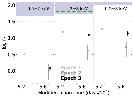
Figure 3: Logarithm of the observed flux in the Chandra soft (0.5–2 keV), hard (2–8 keV), and full (0.5–8 keV) bands in units of $10^{-14}$ erg cm^-2 s^-1 versus modified Julian date for each Chandra observation of PG 2112+059. The shaded area corresponds to the expected range of X-ray fluxes obtained assuming a typical $\hbox{$\alpha_{\rm ox}$}=0.384\times{\rm log}[L_{\rm 2keV}/L_{2500}]$ (see Table 5 of Steffen et al., 2006) and a power-law spectrum with $\Gamma=1.9$. The horizontal dotted line corresponds to the best-fit brightest flux ever obtained (in 1999 with ASCA, MJD$=51481$). The light gray, gray and black colors are associated with epochs 1, 2 and 3, respectively.

3 Results

In this section, we test the significance of the variability of different spectral (UV and X-ray) parameters between two epochs. In order to do this, we calculate the $\chi^{2}$ statistic assuming that the data points are the estimated parameter (with their respective 1$\sigma$ errors), and the model is a constant obtained from the best fit. The $\chi^{2}$ value provides a statistical test of the null hypothesis that the parameter value of each epoch is equal to its best-fitted value. This model has one parameter to fit two data points, thus the $\chi^{2}$ value follows a $\chi^{2}$-distribution with one degree of freedom. From hereafter, we refer to a significant (marginal) change of a parameter between two epochs, when the null hypothesis probability is less than 0.01 (between 0.05 and 0.01). The soft X-ray fluxes (i.e., at energies up to 2 keV) in Epoch 1 are significantly larger than those in the other epochs (see Table 5). Additionally, when Epochs 2 and 3 are compared, although soft X-ray fluxes do not show significant variation, the hard flux presents a marked increase (see Figures 2–3 and Table 5). We also find hardening in the X-ray spectra when Epoch 1 is compared with Epoch 3 with a significant increase in the hardness-ratio (hereafter HR) as seen in Table 5. As compared to the X-rays, the UV continua show only minor variations (see Figure 1 and Table 6), and thus, the multiwavelength changes (measured by $\alpha_{\rm ox}$) between Epoch 1 and the other epochs, are mainly the product of the significant variation in the soft X-ray flux. Additionally, a significantly redder UV spectrum is observed when Epoch 1 is compared with Epochs 2-3 (see $\alpha_{EUV}$ and $\alpha_{FUV}$ in Table 6).

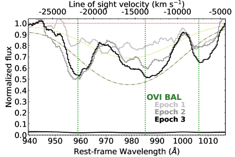
Figure 4: Normalized flux in the O vi BAL region. The light gray, gray and black colors histograms are the STIS spectra observed in epochs 1, 2 and 3, respectively. The lower curve correspond to errors at the 68% confidence level. The three vertical dotted lines indicate line of sight outflow velocities of $-21900$,$-13800$ and $-7500$ km s^-1 around local minima respectively. The dashed and dot-dashed curves correspond to blue-shifted (blue-shift velocity of 16000 km s^-1) partially covered ($C_{f}=0.8$) absorption profiles obtained from cloudy runs with $\log U=-0.8$, turbulent velocity 6500 km s^-1 and column densities $\hbox{log~{}$N_{\rm H}$}=20.1$ and $\hbox{log~{}$N_{\rm H}$}=20.5$ respectively. Figures 4–6 are obtained using boxcar smoothing over 13 pixels for the G140L spectra and 7 pixels for the G230L spectra.

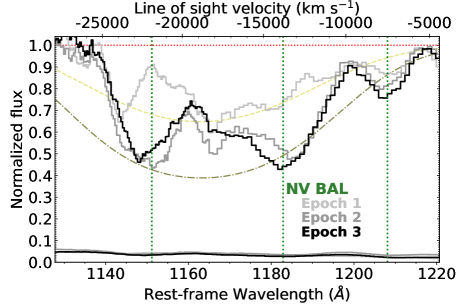
Figure 5: Normalized flux in the Ly$\alpha$-N v BAL region (see legend of Figure 4 for more details).

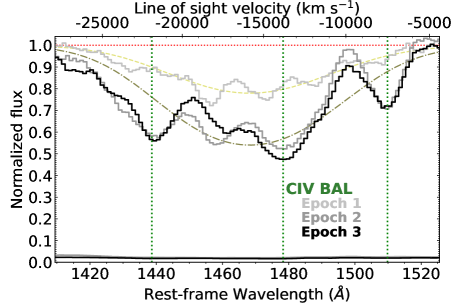
Figure 6: Normalized flux in the C iv BAL region (see legend of Figure 4 for more details).

The observed BALs in the HST spectra are mainly due to the O vi, N v, and C iv line doublets, albeit there are other absorption lines as well that could have secondary contributions in the observed BALs (see §4.1 for details). Hereafter, unless otherwise stated, we assume that the zero velocity for each ion is the absorbing line laboratory wavelength for the blue component of the doublets given by Verner et al. (1994). These wavelengths are 1031.9 Å (O vi), 1238.8 Å (N v), and 1548.2 Å (C iv). Using the fitted model spectra (continuum+ELs) described in §2.3 we obtain the normalized spectra around the O vi, N v, and C iv BALs as shown in Figures 4–6 . In general, for all the BALs observed, Epochs 2 and 3 show more conspicuous absorption than Epoch 1. Additionally, the spectral differences are most pronounced when comparing either Epoch 2 or 3 with Epoch 1. Epochs 2 and 3 show strong differences with Epoch 1 that are concentrated at $\approx 960$ Å  and $\approx 990$ Å for the O vi BAL, at $\approx 1150$ Å and $\approx 1190$ Å  for the N v BAL, and at $\approx 1440$ Å and $\approx 1480$ Å for the C iv BAL. For every ion, when Epoch 2 or 3 are compared with Epoch 1, the zones of variability are more intense at velocities $\approx-22000\>\hbox{km~{}s${}^{-1}$}$ and $\approx-13000\>\hbox{km~{}s${}^{-1}$}$. Epochs 2 and 3 show small differences between each other that seem to be more marked at $\approx 990/1010$ Å ($\approx-12000/-7000\>\hbox{km~{}s${}^{-1}$}$), $\approx 1180$ Å ($\approx-14000\>\hbox{km~{}s${}^{-1}$}$) and $\approx 1460$ Å ($\approx-17000\>\hbox{km~{}s${}^{-1}$}$) for the O vi, N v, and C iv BALs, respectively. The normalized spectra also show a reasonable level of consistency when observed as a function of velocity. For example, the BALs in Epoch 1 appear as relatively featureless profiles in the range of velocities between $-25000$ to $-5000$ km s^-1. On the other hand, the absorption profiles of Epochs 2 and 3 seem to share similar distinguishable features centered at speeds $\sim-22000$, $\sim-14000$ and $\sim-8000$ km s^-1 respectively (see vertical dotted lines in Figures 4–6). As a separate note, an HST FOS observation performed in 1992 shares qualitative spectral similarities with Epochs 2 and 3. In this observation the UV spectral slope of PG 2112+059 was redder, and the EWs of the BALs were greater when compared with Epoch 1 (see Fig. 4 of Gallagher et al., 2004).

Table 7: Equivalent widths of UV BALs

	equivalent-widths			equivalent-width ratios
epoch	O vi	N v	C iv	${\hbox{O {\sc vi}}}/{\hbox{C {\sc iv}}}$	${\hbox{N {\sc v}}}/{\hbox{C {\sc iv}}}$	${\hbox{N {\sc v}}}/{\hbox{O {\sc vi}}}$
(1)	(2)	(3)	(4)	(5)	(6)	(7)
1	10.5$\pm$1.1	16.6$\pm$1.4	12.9$\pm$1.2	0.81$\pm$0.11	1.28$\pm$0.16	1.57$\pm$0.21
2	17.6$\pm$0.9	27.8$\pm$1.0	29.0$\pm$1.4	0.61$\pm$0.04	0.96$\pm$0.06	1.58$\pm$0.10
3	19.7$\pm$0.9	27.3$\pm$1.1	30.0$\pm$1.1	0.66$\pm$0.04	0.91$\pm$0.05	1.39$\pm$0.09

Equivalent Widths (EW) and their errors are obtained from equations 2 and 3 of §3 Col. (1): Observation Epoch. Cols. (2–4): Equivalent widths (in Å) of O vi, N v  and C iv BALs. Cols. (5–7): Equivalent width ratios.

The equivalent width (EW) of an absorption feature is defined as:

$${\rm EW}=\int(1-f(\lambda))d\lambda,$$ (1)

where $f(\lambda)$ is the normalized spectra. This is obtained by adding each pixel contribution through (Kaspi et al., 2002):

$${\rm EW}=\sum_{i}\left(1-\frac{F_{i}}{F_{C}}\right)B_{i},$$ (2)

where $i$ runs through every pixel, $F_{i}$ is the flux in the $i$th pixel, $B_{i}$ is the pixel width (in Å), and $F_{C}$ is the continuum flux. Additionally the EW error is calculated by expanding the errors of the flux in each pixel and the error of the continua, thus obtaining:

$$\Delta{\rm EW}=\sqrt{\left(\frac{\Delta F_{C}}{F_{C}}\sum_{i}\frac{B_{i}F_{i}}{F_{C}}\right)^{2}+\sum_{i}\left(\frac{B_{i}}{F_{C}}\Delta F_{i}\right)^{2}}.$$ (3)

For each of the three BAL features (i.e., O vi, N v, and C iv), valid pixels for EW calculations are those in the range of blueshifted velocities of $3000$ to $25000$ km s^-1, using as reference the wavelength of the O vi 1032, N v 1239, and C iv 1548 blue doublets, respectively. Since the Si iv BAL is not observed, we obtain EW upper limits by multiplying by 2.3 the EW error (upper limit at the $\approx 99$% confidence level), which is obtained assuming $F_{i}=F_{C}$ in equation 3 and the wavelength of the blue doublet of the Si iv 1394 as the reference. These EW upper limits are $\sim 4$ Å for every observation.

For each epoch, the EWs and EW ratios of the observed BALs in the rest-frame of PG 2112+059 are presented in Table 7. From this table, we infer that there is no significant overall difference (within the errors) between the EWs obtained in Epochs 2 and 3. However, Epoch 1 shows weaker EWs in every observed BAL feature when compared either with Epochs 2 or 3 (see Table 7). We do not find any significant change in the EWs ratios between epochs.

Table 8: Spectral properties of BAL features

	O vi (1031.9 Å)				N v (1238.8 Å)				C iv (1548.2 Å)
epoch	$v_{\rm min}$	$v_{\rm max}$	$v_{\rm mean}$	$BI$	$v_{\rm min}$	$v_{\rm max}$	$v_{\rm mean}$	$BI$	$v_{\rm min}$	$v_{\rm max}$	$v_{\rm mean}$	$BI$
(1)	(2)	(3)	(4)	(5)	(6)	(7)	(8)	(9)	(10)	(11)	(12)	(13)
1	$-5222$	$-23136$	$-14391$$\pm$2009	1594$\pm$242	$-10094$	$-24749$	$-16527$$\pm$1960	2136$\pm$199	$-10595$	$-23336$	$-16038$$\pm$1808	1046$\pm$105
2	$-5326$	$-25748$	$-16110$$\pm$996	3900$\pm$226	$-6420$	$-25039$	$-16952$$\pm$799	5414$\pm$154	$-6381$	$-25761$	$-16520$$\pm$958	4626$\pm$213
3	$-5127$	$-23908$	$-14974$$\pm$907	4472$\pm$210	$-6199$	$-24767$	$-16306$$\pm$844	5241$\pm$182	$-6417$	$-27129$	$-15951$$\pm$686	4688$\pm$173

The units of (2–13) are km s^-1. Col. (1): Observation Epoch. Cols. (2–13): $v_{\rm min}$, $v_{\rm max}$, $v_{\rm mean}$ and BI for O vi (Cols. 2–5), N v (Cols. 6–9) and O vi (Cols. 10–13).

We obtain the balnicity index (hereafter BI) using the standard approach of Weymann et al. (1991), i.e., through:

$$BI=\int_{3000}^{25000}\left(1-\frac{f(-v)}{0.9}\right)Cdv,$$ (4)

where $f(v)$ is the normalized spectrum at velocity $v$ in km s^-1 in the rest frame. The BIs starts to count from blueshifted velocities greater than 3000 km s^-1 and $C$ is equal to zero unless the absorption depth in the normalized spectrum is greater than 10% for an span of at least 2000 km s^-1. As in the case of the EW, blueshifted velocities above 25000 km s^-1do not count for the BI calculations. The velocity ranges where we find BAL absorption are $v_{\rm min}$ and $v_{\rm max}$, and we assume that this absorption is present when the spectrum falls below 10% of the continuum level. For each ion, the calculations of BI, $v_{\rm min}$, and $v_{\rm max}$ are obtained using boxcar smoothing over 13 pixels for the G140L spectra and 7 pixels for the G230L spectra (see Table 8). Since the BI index is a modification of the EW, we properly modify equations 2 and 3 to obtain BIs with their errors. We also calculate a mean velocity of each BAL given by

$$\text{$v_{\rm mean}$}=-\frac{\displaystyle\ \int_{3000}^{25000}(1-f(-v))vdv}{\displaystyle\ \int_{3000}^{25000}(1-f(-v))dv},$$ (5)

where $f(v)$ is the normalized spectrum. The calculations of $v_{\rm mean}$ with their error were obtained adding each pixel contribution in a similar fashion as was done when obtaining the EWs. As shown in Table 8, the BIs show similar tendencies as the EWs, and based on the C iv line, PG 2112+059 BIs range between 1000–4700 km s^-1. This range of BIs is consistent with a BI of $\approx 2980$ km s^-1obtained by Brandt et al. (2000) on a FOS/HST observation of PG 2112+059 performed in 1992. Additionally, from Table 8, although some variations of $v_{\rm min}$ and $v_{\rm max}$ are observed, these seem to be associated with changes in the optical depth and not with dynamical variations of the wind. This statement is confirmed by the mean velocity of the outflow ($v_{\rm mean}$), which does not show any significant variations either when we compare between BAL features or observations (as seen in Table 8).

4 Analysis and Discussion

In this section, we analyze possble physical scenarios that could explain our results. In §4.1 we introduce a photoionization model that attempts to constrain basic physical properties of the UV outflow (e.g., the ionization state and hydrogen column density) based on the ranges of the EW and EW ratios presented in the last section. For this subsection, an optically thin BAL medium fully covering the central source is assumed. In §4.2 we analyze an extension §4.1 by incorporating the covering fraction in the modeling of the UV wind. Finally, in §4.3 we discuss the possible connection between the decrease in the soft X-ray emission and the increase in the BAL EWs found in Epochs 1–3.

4.1 cloudy simulations

Under the assumption that the absorbing gas producing the BAL features observed and analyzed in §3 have a common origin, we use cloudy (version C17.vr; Ferland et al., 2017) to analyze the observed equivalent widths and ratios found in Table 7. We perform cloudy simulations assuming a point source AGN-type spectrum incident to an optically thin media. The spectral energy distribution (SED) of the point source spectrum is the agn cloudy model. The specific cloudy command used was AGN 5.5 -2.2 -0.5 0 in which 5.5 is the logarithm of the temperature (in kelvin) of the big blue bump, $-2.2$ is $\alpha_{\rm ox}$, $-0.5$ is the low energy slope of the big blue bump $\alpha_{UV}$, and 0 is the X-ray slope $\alpha_{x}$ (where $\alpha_{x}=-\Gamma+1$). These parameters have been chosen to approximately fit the spectral energy distribution of past and current observations of the X-ray and UV spectra of PG 2112+059 (see Fig. 7). The absorbing medium is given by a layer with total hydrogen column density of $\hbox{${N}_{\rm H}$}=10^{13}~{}\hbox{cm${}^{-2}$}$ fully covering the central source, with solar abundances and a fixed hydrogen density of $n_{\rm H}=10^{8}~{}\hbox{cm${}^{-3}$}$. The chosen value of $n_{\rm H}$ can be varied by at least three orders of magnitude without producing any noticeable effect on the results of our simulations (see e.g. Hamann, 1997). The value of ${N}_{\rm H}$ is chosen in order that the medium is “thin enough" so the most prominent lines that could form BALs have optical depths $\tau_{0}$ in their centers which are significantly less than unity.

The cloudy simulations have been performed varying the values on the ionization parameter of the absorbing layer. The ionization parameter is the ratio of hydrogen ionizing photon density to hydrogen density, i.e.:

$$U=\frac{Q_{\rm H}}{4\pi r^{2}n_{\rm H}c},$$ (6)

where $n_{H}$ is the total hydrogen density. $Q_{H}$ is the rate of hydrogen ionizing photons emitted by the central object given by:

$$Q_{\rm H}=\int_{\nu_{Ry}}^{\infty}\frac{L_{\nu}d\nu}{h\nu},$$ (7)

where $\nu_{Ry}$ is the frequency for photons with energies of 1 Rydberg ($Ry$).

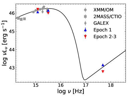
Figure 7: SED used for our cloudy simulations. For reference we plot photometric data from: XMM-Newton Optical Monitor (circles; from Schartel et al., 2007), 2MASS/CTIO (squares; from Skrutskie et al., 2006), GALEX (diamonds; from Bianchi et al., 2014), and our observations (with triangles for Epoch 1 and inverted triangles obtained from the weighted mean X-ray and UV fluxes from Epoch 2 and 3 in Tables 5 and 6).

In the optically thin regime for a fixed value of the ionization parameter and metallicity, the equivalent-width of an absorption line associated to the ion $j$ of column density $N_{j}$ should satisfy:

$${\rm EW}\propto N_{j}\propto\hbox{${N}_{\rm H}$}.$$ (8)

In particular, $N_{j}$ can be obtained through the following expression:

$$N_{j}\approx\frac{m_{e}c^{2}}{\pi e^{2}f\lambda_{0}^{2}}{\rm EW},$$ (9)

where $f$ is the oscillator strength and $\lambda_{0}$ is the laboratory wavelength of an absorption line associated to the ion $j$. Additionally, for Gaussian line profiles the optical depth at the line center of an absorption line produced by an ion $j$ is:

$$\tau_{0}\approx\frac{{\rm EW}\,c}{\sqrt{\pi}\,b\,\lambda_{0}},$$ (10)

where $b=\sqrt{2kT/m_{j}}$ is the most probable thermal velocity. If we assume that the BALs are the added contribution of blue-shifted optically thin layers, our model can be properly scaled to represent the BAL medium. From the curves presented in Figures 4–6, if we assume $C_{f}=1$ we confirm that the BAL medium maximum optical depth is $\tau_{\lambda}(\rm max)\lesssim 0.5$, and thus, we expect that our model can be used to estimate the ionization state and column density of the ions that produce the BALs. By comparing these ion column densities with those obtained in our cloudy runs (with log $N_{\rm H}$=13), through equations 8 and 9, we can also extrapolate column densities of other ions or elements that do not necessarily have observed spectral signatures (for example ${N}_{\rm H}$). For partially covered outflows ($C_{f}<1$), which are commonly seen in BAL quasars (see e.g., Arav et al., 1999; Dunn et al., 2012; Leighly et al., 2019), our model can be extended to provide useful insights into the ionization and column densities of the wind as described in §4.2.

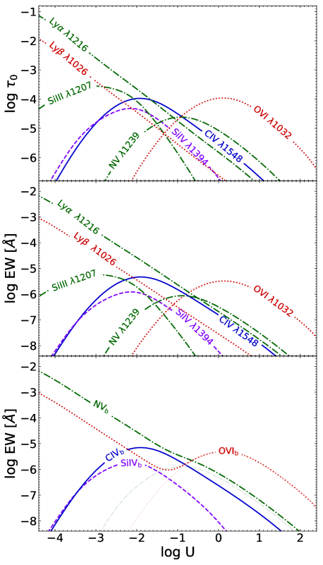
Figure 8: Upper panel: Logarithm of line-center optical depths versus logarithm of the ionization parameter. Middle panel: Logarithm of the equivalent width versus logarithm of the ionization parameter. Lower panel: Logarithm of the combined equivalent width (EW) versus logarithm of the ionization parameter for line blending BAL regions. In the upper and middle panels the lines marked correspond to the most prominent lines that are likely found in the BALs of the HST/STIS spectra. In all the panels the dotted, dash-dotted, dashed and full lines indicate lines belonging to the $\rm OVI_{b}$, $\rm NV_{b}$, $\rm SiIV_{b}$ and $\rm CIV_{b}$ blends, respectively (see main text for more details). In the lower panel in a whiter tone the combined EW of the O vi 1032,1038 (dotted-line), N v 1239,1243 (dash-dotted) line doublets are marked. This figure is generated through cloudy simulations of a point source AGN spectrum incident on an optically thin layer with a column density of $10^{13}\,\hbox{cm${}^{-2}$}$.

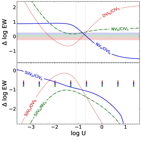
Figure 9: Logarithm of the equivalent width ratios of two line blends versus logarithm of the ionization parameter. Upper panel: The dotted, dash-dotted, and full lines indicate the $\rm OVI_{b}/CIV_{b}$, $\rm NV_{b}/CIV_{b}$, and $\rm NV_{b}/OVI_{b}$ EWs ratios, respectively. The red, green and blue horizontal bands represent the observed ranges of (in all Epochs) $\rm OVI_{b}/CIV_{b}$, $\rm NV_{b}/CIV_{b}$, and $\rm NV_{b}/OVI_{b}$ ratios (from Table 7). Lower panel: the dotted, dash-dotted, and full lines indicate the $\rm SiIV_{b}/OVI_{b}$, $\rm SiIV_{b}/NV_{b}$, and $\rm SiIV_{b}/CIV_{b}$ EWs ratios respectively. The red, green and blue downward arrows mark the maximum $\rm SiVb/OVI_{b}$, $\rm SiVb/NV_{b}$ and $\rm SiVb/CIV_{b}$ EW ratio upper limits in our observations. Both panels are generated through cloudy simulations of a point source AGN spectrum incident on an optically thin layer with a column density of $10^{13}\hbox{cm${}^{-2}$}$. The vertical dotted-line band marks the expected $\log U$ range of the BAL medium (see §4.1).

The absorption lines that we analyze are those that have significant signatures in the wavelength range of the HST/STIS spectrum. Additionally, these lines must cover the ionization states where the C iv lines are significant. The most important of these lines are the O vi 1032,1038, N v 1239,1243, Si iv 1394,1403 and C iv 1548,1551 doublets. There are other lines that should have signatures in the spectral and ionization ranges of consideration; these are the Ly$\alpha$ 1216, Ly$\beta$ 1026, and the Si iii 1207 lines. Given the wavelengths of these lines, we likely expect to find four blended sets of lines that could form BALs in our observations. The first, identified as the $\rm OVI_{b}$ blend is produced by the Ly$\beta$ line and the O vi doublet. The second blend, identified as the $\rm NV_{b}$ blend is produced by the Ly$\alpha$, Si iii lines and the N v  doublet. Finally, the third and fourth, identified as the $\rm SiIV_{b}$ and $\rm CIV_{b}$ blends are produced by the Si iv and C iv doublets, respectively.

In Figure 8 we show the optical depth at the line center $\tau_{0}$ (upper panel) and EW (middle panel) as a function of ionization parameter for the blue line of the O vi, Si iv, N v and C iv doublet with the Ly$\alpha$, Ly$\beta$, and the Si iii lines. In the lower panel of Figure 8 we show the logarithm of the added EWs of each line blend. To differentiate between line blends, in Figure 8 each line in a particular blend is marked with a distinctive line style. The upper panel of this figure shows that all the lines have values of $\tau_{0}$ well below unity, thus confirming the fact that we are analyzing optically thin lines. For our set of parameters, Figure 8 indicates the ionization ranges where each line is contributing to potentially form a BAL. As we see in §3, our observations show prominent C iv BAL signatures with no evidence of Si iv BAL features. Thus, if the BALs are produced by a medium with a narrow range of ionization states, we expect that $\log U\gtrsim-1$. Additionally, we expect that $\log U\lesssim 1$ in order to be able to observe a significant C iv BAL or N v BAL as compared to the O vi BAL . Therefore, in general we expect an outflow with $-1\lesssim\log U\lesssim 1$, although a more refined ionization parameter range is obtained from analyzing the EW ratios as described in the following paragraphs. In this ionization parameter range a comparison of the middle and lower panels in Figure 8 confirms that the most prominent lines producing BALs in our observations are the blue components of C iv, O vi and N v doublets.

In Figure 9 the logarithms of the EW ratios of two different line blends as a function of $U$ are shown. The curves in the upper panel of Figure 9 correspond to ratios between the EWs of blends that could produce the observed BALs (i.e., OVIb, NVb, and CIVb blends). Additionally, the curves in the lower panel correspond to ratios between the EWs of the SiIVb blend and the OVIb, NVb, and CIVb blends, respectively. In the upper panel of Figure 9 we have marked horizontal bands that correspond to the maximum and minimum EW ratios obtained from Table 7. A simple observation of these bands indicates that there is no particular value of the ionization parameter that produces all the observed ratios in Table 7. Additionally, the upper panel of Figure 9 shows that the observed values of the $\rm NV_{b}$/$\rm CIV_{b}$ EW ratios are below the full-line curve. Thus, the discrepancies between our model and the observed EW ratios might be due to unknown complexity of the outflow, like variations from solar abundances of Oxygen, Nitrogen and Carbon and/or gradients in the ionization state through the outflow. There could also be discrepancies due to the assumption of optical thinness of our model, although we expect these should not be important as described in §4.2.

The fact that the observed NVb/CIVb EW ratios are lower than expected from our model might be attributed to subsolar N/C abundance ratios as observed in quasar HE 0141–3932 (Reimers et al., 2005). Since we cannot observe individual lines in the outflow and thus cannot estimate the relative abundances of O, N and C, in order to estimate a range for the ionization parameter of the wind, we add an error of 0.3 dex in the logarithm of the observed EW ratios. This error is close to what is expected from the dispersion of relative abundances of O, N and C in extragalactic H ii regions at nearly solar metallicities (e.g., Esteban et al., 2009; Berg et al., 2016). Based on the expanded error bands in the EW ratios, we obtain from the curves in Figure 9 that $-1.2\lesssim\log U\lesssim-0.7$, $-1.8\lesssim\log U\lesssim-0.2$, and $-1.1\lesssim\log U\lesssim-0.5$ from the O vi/C iv, N v/C iv and N v/O vi ratios, respectively. Additionally, by comparing the observed Si iv ratios upper limits with the curves in the lower panel of Figure 9, we obtain $\log U\gtrsim-1.1$, and thus, we expect a range of the ionization outflow parameter $-1.1\lesssim\log U\lesssim-0.7$. Assuming that the ionization parameter is uniformly distributed in $[-1.1,-0.7]$ , and using the tables generated by our cloudy simulations, we obtain logarithms of relative abundance ratios with respect to hydrogen of $-4.21\pm 0.14$, $-4.40\pm 0.05$, $-4.51\pm 0.12$ for O vi, N v and C iv respectively. From equations 8 and 9, the abundance ratios obtained can be used to estimate (from the O vi, N v, and C iv ion column densities) the BALs hydrogen column densities.

Using the observed EW of each BAL in Table 7 we obtain an approximation of the column densities of the O vi, N v, and C iv ions through equation 9. For this we assume that the EW of each observed BAL is produced by the added EWs of the O vi, N v, and C iv doublets respectively. Additionally, from the estimated relative abundances of ions with respect to hydrogen we estimate ${N}_{\rm H}$ column densities from each ion, which are shown in Table 9. As this table indicates, the medium that produces the BALs has $\hbox{log~{}$N_{\rm H}$}\sim 20$ in Epoch 1 and its column density increases by $\approx 0.3$ dex from Epoch 1 to Epochs 2-3.

Table 9: Observed column densities of UV BALs

	logarithm of ion column densities			logarithm of h column densities
epoch	O vi	N v	C iv	O vi	N v	C iv
(1)	(2)	(3)	(4)	(5)	(6)	(7)
1	15.75$\pm$0.04	15.72$\pm$0.04	15.33$\pm$0.04	19.96$\pm$0.15	20.11$\pm$0.06	19.84$\pm$0.13
2	15.97$\pm$0.02	15.94$\pm$0.01	15.68$\pm$0.02	20.19$\pm$0.14	20.34$\pm$0.05	20.20$\pm$0.12
3	16.02$\pm$0.02	15.93$\pm$0.02	15.69$\pm$0.01	20.23$\pm$0.14	20.33$\pm$0.05	20.21$\pm$0.12

Col. (1): Observation Epoch. Cols. (2–4): Logarithm of ion column densities (in cm^-2) obtained using equation 9 from the equivalent widths (EWs) of the O vi, N v  and C iv BALs. Cols. (5–7): Logarithm of hydrogen column densities as obtained from columns (2–4) and the ion abundances ratios with respect to hydrogen estimated by our thin layer cloudy model (as described in §4.1).

Equation 6 can be used to obtain $r_{UV}$, the distance from a central emitting source to the observed UV BAL wind. In view of our observations, we assume that $-1.1\lesssim\log U\lesssim-0.7$ and $Q_{H}=5.6\times 10^{56}~{}{\rm s}^{-1}$ from the SED obtained in Figure 7. Additionally, based on observations of BALs, mini-BALs and NALs, the electron density of the outflow $n_{e}$ should lie between $3\lesssim\log n_{e}\lesssim 10$ (e.g., de Kool et al., 2001; Hamann et al., 2011; Misawa et al., 2016; Xu et al., 2019), with $n_{\rm H}\approx n_{e}$. Based on these assumptions $r_{UV}$ is within $[10^{3}-10^{7}]R_{S}$ ($[0.1-1000]~{}{\rm pc}$), where $R_{S}$ is obtained assuming a black hole mass of $M_{\rm BH}\approx 10^{9}M_{\odot}$ (Vestergaard & Peterson, 2006).

4.2 Optical Depth Fits

In this section, we estimate the BAL ion column densities by performing fits on the optical depths. This is done in order to analyze outflows that are not necessarily optically thin nor are totally covering the central source. The fits are performed by first transforming the normalized spectra to an optical depth profile as a function of wavelength ($\tau_{\lambda}$). The optical depth BAL profiles, assumed to be produced by the O vi, N v, and C iv  line doublets (as in §4.1), are deblended using the methodology described in Junkkarinen et al. (1983). Using this approach the $\tau_{\lambda}$ profile is transformed to a single line with an oscillator strength of $f_{*}=f_{b}+f_{r}$ and a laboratory wavelength given by $\lambda_{*}=(f_{b}\lambda_{b}+f_{r}\lambda_{r})/(f_{b}+f_{r})$, where $f_{b}$ ($f_{r}$) is the oscillator strengths of the blue (red) doublet and $\lambda_{b}$ ($\lambda_{r}$) is the laboratory wavelengths of the blue (red) doublet. Once deblended, each BAL profile is fitted as function of velocity using Gaussian profiles i.e.,

$$\tau_{v}=\tau_{0}\exp(-((v-v_{0})/b)^{2}),$$ (11)

where $\tau_{0}$ is an estimation of the maximum optical depth of the profile. The ion column density of a single line absorption profile can be obtained from the optical depth velocity profile through the following expression:

$$N_{j}=\frac{m_{e}c}{\pi e^{2}f_{*}\lambda_{*}}\int\tau_{v}\,dv,$$ (12)

where $\int\tau_{v}\,dv=\sqrt{\pi}\,\tau_{0}\,b$ for a Gaussian profile. Therefore, using equation 12 we show in Table 10 the column densities of the O vi, N v and C iv ions using Gaussian fits on the optical depth profiles of each observation. Additionally, in Table 10, we show the estimated hydrogen column densities using the relative ion abundance ratios with respect to the hydrogen obtained in §4.1. For $C_{f}=1$, the results in Table 10 (as expected) are very similar to those of Table 9. For $C_{f}<1$, which is the case of an absorber partially covering the emitting source, the observed and true optical depths of an absorption line are obtained from:

$$\exp(-\tau_{\lambda}^{\rm obs})=(1-C_{f})+C_{f}\exp(-\tau_{\lambda}^{\rm true}).$$ (13)

Since $\tau_{\lambda}^{\rm true}$ grows monotonically with column density, in absence of constraints on the column density, the assumption of $C_{f}=1$ results in column densities that are lower limits. In Table 10 we have performed again Gaussian fits to the deblended ionic profiles but now with $C_{f}=0.8$ and 0.6. The case of $C_{f}=0.6$ is a rough estimate of the minimum value expected from Epochs 2 and 3. From Table 10, as expected, the column densities and maximum optical depths ($\tau_{0}$) vary approximately inversely proportional with $C_{f}$. Additionally, from this table, we conclude that for a given BAL profile if $C_{f}$ is close to its expected minimum then $\tau_{0}\gtrsim 1$. For this particular case, i.e. of saturated line profiles, our model might not give reliable estimates of $U$ and/or ${N}_{\rm H}$.

The approach used to describe the UV BAL winds in §4.1 and this section is mainly based on constraining the medium ionization parameter and describing ion column densities of each BAL. This methodology, although simple should give us reliable constraints on the expected column densities and the ionization state of the wind. To clarify this better, we generate two cloudy runs motivated by the optical depth Gaussian fits in the case of $C_{f}=0.8$. Both runs are from a layer with solar abundance, with ionization parameter at the illuminated face $\log U=-0.8$, and turbulent velocity $v_{\rm turb}=6500~{}\hbox{km~{}s${}^{-1}$}$. The difference in the runs are the chosen values of column densities which are $\hbox{log~{}$N_{\rm H}$}=20.1$ and $\hbox{log~{}$N_{\rm H}$}=20.5$ respectively. The chosen value of $U$ is within the expected for the UV BAL medium, $v_{\rm turb}$ is close to the average value of the estimated velocity dispersions of the Gaussian fits ($b$ parameter in equation 11), and the values of log $N_{\rm H}$ are close to the average values estimated for Epoch 1 and Epochs 2-3 (for $C_{f}=0.8$ in Table 10). The absorption spectra from these cloudy runs are then corrected for partial covering (using equation 13 with $C_{f}=0.8$) and blue-shifted with a blue-shifted velocity of 16000 km s^-1. This velocity is close to the average Gaussian central velocities ($v_{o}$ in equation 11) obtained from the fits. The resulting absorption profiles are shown in Figures 4–6. By comparing these curves with the observed profiles, and given the simplicity of our model assumptions, we find a good agreement with the observations. Note that similar absorption profiles to those presented in Figures 4–6 can be obtained for the case of $C_{f}=1$ and $C_{f}=0.6$. The use of more sophisticated photoionization models (e.g., Leighly et al., 2018, 2019) requires a clearer definition of the continuum at rest-frame wavelengths $\lesssim 1200$ Å, and additional evidence of spectral features (not found in this work) that could provide tighter constraints in the covering fraction and/or the chemical abundance of the BALs medium.

Table 10: Column densities and maximum optical depths from deblended Gaussian fits to BAL optical depth profiles

	logarithm of ion column densities			logarithm of h column densities			Fitted values of $\tau_{0}$
epoch	O vi	N v	C iv	O vi	N v	C iv	O vi	N v	C iv
(1)	(2)	(3)	(4)	(5)	(6)	(7)	(8)	(9)	(10)
	covering fraction Cf= 1.00
1	15.83$\pm$0.04	15.72$\pm$0.04	15.38$\pm$0.02	20.04$\pm$0.15	20.12$\pm$0.06	19.89$\pm$0.12	0.23$\pm$0.01	0.32$\pm$0.02	0.24$\pm$0.01
2	16.11$\pm$0.05	16.02$\pm$0.03	15.79$\pm$0.03	20.32$\pm$0.15	20.42$\pm$0.06	20.30$\pm$0.12	0.38$\pm$0.02	0.62$\pm$0.03	0.56$\pm$0.02
3	16.12$\pm$0.04	16.00$\pm$0.03	15.81$\pm$0.03	20.33$\pm$0.15	20.40$\pm$0.06	20.32$\pm$0.12	0.46$\pm$0.03	0.61$\pm$0.03	0.53$\pm$0.02
	covering fraction Cf= 0.80
1	15.93$\pm$0.05	15.84$\pm$0.04	15.49$\pm$0.02	20.14$\pm$0.15	20.24$\pm$0.07	20.00$\pm$0.12	0.30$\pm$0.02	0.42$\pm$0.03	0.31$\pm$0.01
2	16.23$\pm$0.05	16.15$\pm$0.03	15.92$\pm$0.03	20.44$\pm$0.15	20.55$\pm$0.06	20.43$\pm$0.12	0.51$\pm$0.03	0.85$\pm$0.05	0.76$\pm$0.03
3	16.24$\pm$0.05	16.14$\pm$0.03	15.93$\pm$0.03	20.45$\pm$0.15	20.54$\pm$0.06	20.44$\pm$0.12	0.62$\pm$0.04	0.84$\pm$0.05	0.72$\pm$0.03
	covering fraction Cf= 0.60
1	16.08$\pm$0.05	15.99$\pm$0.04	15.63$\pm$0.02	20.29$\pm$0.15	20.39$\pm$0.07	20.14$\pm$0.12	0.42$\pm$0.03	0.61$\pm$0.04	0.44$\pm$0.01
2	16.40$\pm$0.06	16.37$\pm$0.04	16.10$\pm$0.03	20.61$\pm$0.15	20.77$\pm$0.07	20.61$\pm$0.12	0.77$\pm$0.05	1.43$\pm$0.10	1.22$\pm$0.05
3	16.42$\pm$0.05	16.35$\pm$0.04	16.12$\pm$0.03	20.63$\pm$0.15	20.75$\pm$0.07	20.63$\pm$0.12	0.99$\pm$0.07	1.44$\pm$0.11	1.20$\pm$0.07

Col. (1): Observation Epoch. Cols. (2–4): Logarithm of ion column densities (in cm^-2) obtained using equation 12 on optical dephs obtained through Gaussian fits of the deblended optical depth profiles of the O vi, N v  and C iv BALs. Cols. (5–7): Logarithm of hydrogen column densities as obtained from columns (2–4) and the ion abundances ratios with respect to hydrogen as described in §4.1. Cols. (8–10) maximum optical depth from Gaussian fits of the deblended optical depth profiles of the O vi, N v  and C iv BALs.

4.3 Is there a Connection between variability of the BALs and the X-rays?

With a limited sample of observations, we are not able to establish any conclusive argument regarding an X-ray wind connection in PG 2112+059. However, our analysis has revealed some trends that could shed light on what to expect for future observations. The most relevant tendency shown in our observations is that a weakening in the soft X-ray flux could be associated with an increase of the EW of the BALs (see Figures 3–6). The mean velocities of the BALs did not change significantly in our observations; thus, we do not find evidence that the X-rays are connected with the acceleration mechanism of the UV wind.

If the BALs are produced from an optically thin medium, fully covering the central source, the increase in the EW could be due to a growth in the column density of the wind, which doubled between Epoch 1 and Epochs 2-3 (as seen in §4.1 and §4.2). Therefore, a weakening in the X-rays could be associated with a more massive outflow. In the case of a partially covered outflow, the EW increase of the BALs might be also linked to a growth in the covering fraction of the wind. As noted in §3 the increase in EW of the BALs is also associated with a redder UV spectra as measured by $\alpha_{EUV}$ and $\alpha_{FUV}$ (see Table 6). This change of the UV spectra may be related to a decrease of the wind inclination with respect to the line of sight (Baskin et al., 2013). A redder UV spectrum might also be a consequence of an increase in the column density (mass) of the outflow. The combined effect of a more massive and/or less inclined wind might produce an increase in the covering fraction and/or the column density. Note that if the UV wind is partially covering the central source, then the BAL column densities of $\hbox{log~{}$N_{\rm H}$}\sim 20$ obtained in §4.1 are interpreted as lower limits (see Table 10).

Epoch 2 corresponds to the weakest state ever recorded in X-rays. The variability in the X-rays between Epoch 1 and Epoch 2-3 could be interpreted as an increase in the column density of the shield (see Table 4). Unfortunatelly, our new X-ray observations have low S/N, and thus, they are not sufficient to give any conclusive statement. From Saez et al. (2012), when comparing past X-ray observations of PG 2112+059, Epoch 1 is close to average X-ray brightness. Additionally, in the ASCA observation performed in 1999 (hereafter identified as Epoch 0; Gallagher et al., 2001), which corresponds to the brightest X-ray observation registered, the 0.5–2 keV X-ray flux is approximately 10 times greater than that of Epoch 1 (see Figure 3). For the brightest X-ray observation, a simple absorbed power law model with $\hbox{log~{}$N_{\rm H}$}\sim 22$ gives a plausible fit to the data (Gallagher et al., 2001; Saez et al., 2012). In conclusion, a shielding layer with a varying log $N_{\rm H}$ from $\sim\,22.0$ to $\sim\,23.0$ might at least explain in part the strong X-ray variability that this source has. The premise of a shield layer with varying column density is also reinforced by the observed values of the 2 keV rest-frame monochromatic fluxes of PG 2112+059. To demonstrate this, we assume that the intrinsic (unabsorbed) monochromatic flux at 2 keV is $f_{\rm 2keV}\approx 11\times 10^{-31}\hbox{erg~{}cm${}^{-2}$~{}s${}^{-1}$}$, which is obtained assuming that the 2500 Å  luminosity is given by the weighted average of Epochs 1–3 and the 2 keV luminosity is from equation 3 of Just et al. (2007). We further assume that every X-ray  observation is a product of an APL model with a varying column density and a fixed photon index ($\Gamma=1.9$). Therefore, with $f_{\rm 2keV}\approx 8\times 10^{-31}\hbox{erg~{}cm${}^{-2}$~{}s${}^{-1}$}$ for the brightest X-ray observation (Epoch 0; see Table 9 from Saez et al., 2012), and the monochromatic 2 keV rest-frame fluxes in Table 5, we estimate $\hbox{log~{}$N_{\rm H}$}\approx 22.0$, 22.8 and 22.9 for Epoch 0, Epoch 1 and Epoch 2-3, respectively. As described in §2.2, we expect the X-ray absorption of PG 2112+059 is more complex than that obtained from an APL model. However, under the assumption that the intrinsic X-ray emission does not vary significantly, the APL model should provide good approximations to the column densities that produce the observed changes in soft X-ray emission.

In the wind-shield scenario (Murray et al., 1995; Gallagher & Everett, 2007), the UV wind is attributed to the outermost portions of the wind while the X-ray shield to the innermost zones of the wind. As stated in §4.1, the UV wind should be at distances from the central source of $r_{\rm UV}\gtrsim 1000R_{S}$. Given the X-ray variability found between Epochs 2 and 3 of $\sim\!5$ months in the rest-frame, and assuming a dynamic shield, a coherent light crossing time argument gives a distance to the central source of $r_{\rm X}\lesssim 1000R_{S}$ (where $M_{\rm BH}\approx 10^{9}M_{\odot}$ is assumed; Vestergaard & Peterson, 2006). Thus, we expect that the absorption in X-rays is produced by a different medium than that producing the UV BAL features. Based on other observations of BAL quasars, we might expect X-ray variability associated to shield signatures on time scales shorter than 5 months in the rest-frame  (e.g., Chartas et al., 2009; Reeves et al., 2020). Under a wind-shield scenario interpretation, a change in the inclination and/or mass of the wind could produce an increment in the column density and/or the covering fraction. Associated to these changes, we also expect a nearly contemporaneous effect in the inner zone of the wind, as observed with a likely increase in the column density of the shield after Epoch 1. In our observations, we do not detect significant changes in the EW ratios of the observed BALs, and thus, we cannot establish if the increase in EWs is associated with changes in the ionization state of the wind. If we assume a shielded wind-scenario in an observation where the X-ray emission flux rises to a close to brightest state, we likely expect less massive winds and changes in the incident SED that could indicate variation in the ionization state of the wind (i.e., variability in the EW ratios).

Based on this analysis, it would be fundamental to perform a multi-wavelength monitoring campaign of this source to confirm or reject the trends found in this work. At this time, it is not possible to elucidate if a complex absorption or simply an intermittent X-ray source is producing the strong variability that this source shows. This dilemma might be resolved with long exposure NuSTAR observations, in order to further constrain the model associated with the fast and dramatic X-ray variability of PG 2112+059. As described in this work, albeit our results are preliminary, a shielded wind model seems to give a plausible explanation to our HST/Chandra spectra.

5 Summary and Conclusions

In this work, we analyze three sets of Chandra observations each with a contemporaneous HST STIS spectra (Epochs 1–3) of PG 2112+059. Epoch 1 was performed in 2002, while Epochs 2 and 3 were performed in 2014–2015 and separated by approximately nine months. Our main conclusions are the following:

1. There is significant X-ray spectral hardening between Epoch 1 and Epoch 3. The soft X-ray flux ($\lesssim\!2$ keV) does not change significantly between Epochs 2 and 3. Additionally, the 0.5–2 keV flux is reduced by approximately one third when Epoch 1 is compared either with Epoch 2 or Epoch 3.

2. The HST  UV spectra exhibit BAL features that are likely associated with the O vi 1032,1038, N v 1239,1243, and C iv 1548,1551 doublets. These observations, in general show that Epoch 1 is significantly distinct from either Epoch 2 or Epoch 3. Additionally, Epoch 3 has only minor changes in relation to Epoch 2. When Epoch 1 is compared with Epochs 2-3, the EWs of the BALs are found to increase and the UV spectral slope becomes redder.

3. Under the assumption that BALs are produced by an optically thin medium fully covering the source, we estimate hydrogen column densities of $\sim 10^{20}\hbox{cm${}^{-2}$}$ for Epoch 1 that increase by a factor of approximately two for Epoch 2-3. If the medium is partially covered ($C_{f}<1$), the outflow column densities obtained assuming $C_{f}=1$ become lower limits and the covering fraction might be also contributing to the changes of EWs. In conclusion, the increasing EWs can be explained by an increase in column densities and/or covering fractions. These changes accompanied by a redder UV spectrum might be indicating a decrease in the inclination of the outflow along the line of sight and/or an increase in the wind mass. The EW ratios of the C iv, N v, and O vi BALs do not change significantly between observation Epochs, implying that the BALs medium ionization parameter is stable.

4. The decrease in the soft ($\lesssim 2$ keV) X-ray flux, that is produced between Epoch 1 and Epoch 2-3, is possibly associated with an increase in the absorption of the shield. This growth is close to contemporaneous with increments of the BALs EWs.

The analysis of the X-ray/UV spectra of PG 2112+059, provide support for the wind-shield scenario model of BAL winds. A future multiwavelength long-term monitoring campaign of this source in combination with a more sophisticated UV spectral analysis (e.g., with SimBAL; Leighly et al., 2018) would be of interest to confirm or reject the conclusions obtained here.

6 Acknowledgements

Support for this work was provided by the National Aeronautics and Space Administration through Chandra Award Number GO5-16119X issued by the Chandra X-ray Observatory Center, which is operated by the Smithsonian Astrophysical Observatory for and on behalf of the National Aeronautics Space Administration under contract NAS8-03060. Support for Program number HST-GO-13948.001-A was provided by NASA through a grant from the Space Telescope Science Institute, which is operated by the Association of Universities for Research in Astronomy, Incorporated, under NASA contract NAS5-26555. We acknowledge support from ANID grants CATA-Basal AFB-170002 (FEB), FONDECYT Regular 1190818 (FEB), 1200495 (FEB) and Millennium Science Initiative Program - ICN12_009 (FEB). This work was partially supported by JSPS KAKENHI Grant Number 21H01126. SCG acknowledges support from the Natural Science and Engineering Research Council of Canada.

7 Data Availability

The scientific results reported in this article are based on publicly available observations made by the Chandra X-ray Observatory and the Hubble Space Telescope (HST). The list of Chandra  observations IDs (ObsIDs) are: 3011, 17148, and 17553. Additionally, the HST observations are from Proposal IDs 13948 and 9277.

References

- Arav et al. (1999) Arav, N., Becker, R. H., Laurent-Muehleisen, S. A., et al. 1999, ApJ, 524, 566
- Arav et al. (2013) Arav, N., Borguet, B., Chamberlain, C., Edmonds, D., & Danforth, C. 2013, MNRAS, 436, 3286
- Arnaud (1996) Arnaud, K. A. 1996, Astronomical Society of the Pacific Conference Series, Vol. 101, XSPEC: The First Ten Years, ed. G. H. Jacoby & J. Barnes, 17
- Barlow (2004) Barlow, R. 2004, ArXiv Physics e-prints, physics/0406120
- Baskin et al. (2013) Baskin, A., Laor, A., & Hamann, F. 2013, MNRAS, 432, 1525
- Berg et al. (2016) Berg, D. A., Skillman, E. D., Henry, R. B. C., Erb, D. K., & Carigi, L. 2016, ApJ, 827, 126
- Bianchi et al. (2014) Bianchi, L., Conti, A., & Shiao, B. 2014, Advances in Space Research, 53, 900
- Bostroem & Proffitt (2011) Bostroem, K. A., & Proffitt, C. 2011, STIS Data Handbook v. 6.0
- Brandt et al. (2000) Brandt, W. N., Laor, A., & Wills, B. J. 2000, ApJ, 528, 637
- Broos et al. (2010) Broos, P. S., Townsley, L. K., Feigelson, E. D., et al. 2010, ApJ, 714, 1582
- Capellupo et al. (2013) Capellupo, D. M., Hamann, F., Shields, J. C., Halpern, J. P., & Barlow, T. A. 2013, MNRAS, 429, 1872
- Cash (1979) Cash, W. 1979, ApJ, 228, 939
- Chartas et al. (2003) Chartas, G., Brandt, W. N., & Gallagher, S. C. 2003, ApJ, 595, 85
- Chartas et al. (2002) Chartas, G., Brandt, W. N., Gallagher, S. C., & Garmire, G. P. 2002, ApJ, 579, 169
- Chartas et al. (2009) Chartas, G., Saez, C., Brandt, W. N., Giustini, M., & Garmire, G. P. 2009, ApJ, 706, 644
- Crenshaw et al. (2003) Crenshaw, D. M., Kraemer, S. B., & George, I. M. 2003, ARA&A, 41, 117
- de Kool et al. (2001) de Kool, M., Arav, N., Becker, R. H., et al. 2001, ApJ, 548, 609
- Dunn et al. (2012) Dunn, J. P., Arav, N., Aoki, K., et al. 2012, ApJ, 750, 143
- Esteban et al. (2009) Esteban, C., Bresolin, F., Peimbert, M., et al. 2009, ApJ, 700, 654
- Fabian (2012) Fabian, A. C. 2012, ARA&A, 50, 455
- Ferland et al. (2017) Ferland, G. J., Chatzikos, M., Guzmán, F., et al. 2017, RMxAA, 53, 385
- Filiz Ak et al. (2014) Filiz Ak, N., Brandt, W. N., Hall, P. B., et al. 2014, ApJ, 791, 88
- Fukumura et al. (2010) Fukumura, K., Kazanas, D., Contopoulos, I., & Behar, E. 2010, ApJL, 723, L228
- Gallagher et al. (2001) Gallagher, S. C., Brandt, W. N., Laor, A., et al. 2001, ApJ, 546, 795
- Gallagher et al. (2004) Gallagher, S. C., Brandt, W. N., Wills, B. J., et al. 2004, ApJ, 603, 425
- Gallagher & Everett (2007) Gallagher, S. C., & Everett, J. E. 2007, in Astronomical Society of the Pacific Conference Series, Vol. 373, The Central Engine of Active Galactic Nuclei, ed. L. C. Ho & J.-W. Wang, 305
- Gehrels (1986) Gehrels, N. 1986, ApJ, 303, 336
- Gibson et al. (2009) Gibson, R. R., Jiang, L., Brandt, W. N., et al. 2009, ApJ, 692, 758
- Güver & Özel (2009) Güver, T., & Özel, F. 2009, MNRAS, 400, 2050
- Haehnelt & Rees (1993) Haehnelt, M. G., & Rees, M. J. 1993, MNRAS, 263, 168
- Hall et al. (2011) Hall, P. B., Anosov, K., White, R. L., et al. 2011, MNRAS, 411, 2653
- Hall et al. (2002) Hall, P. B., Anderson, S. F., Strauss, M. A., et al. 2002, ApJS, 141, 267
- Hamann (1997) Hamann, F. 1997, ApJS, 109, 279
- Hamann et al. (2018) Hamann, F., Chartas, G., Reeves, J., & Nardini, E. 2018, MNRAS, 476, 943
- Hamann et al. (2011) Hamann, F., Kanekar, N., Prochaska, J. X., et al. 2011, MNRAS, 410, 1957
- Hewett & Foltz (2003) Hewett, P. C., & Foltz, C. B. 2003, AJ, 125, 1784
- Hopkins et al. (2006) Hopkins, P. F., Hernquist, L., Cox, T. J., et al. 2006, ApJS, 163, 1
- Junkkarinen et al. (1983) Junkkarinen, V. T., Burbidge, E. M., & Smith, H. E. 1983, ApJ, 265, 51
- Just et al. (2007) Just, D. W., Brandt, W. N., Shemmer, O., et al. 2007, ApJ, 665, 1004
- Kalberla et al. (2005) Kalberla, P. M. W., Burton, W. B., Hartmann, D., et al. 2005, A&A, 440, 775
- Kaspi et al. (2002) Kaspi, S., Brandt, W. N., George, I. M., et al. 2002, ApJ, 574, 643
- Korista et al. (1997) Korista, K., Baldwin, J., Ferland, G., & Verner, D. 1997, ApJS, 108, 401
- Kormendy & Ho (2013) Kormendy, J., & Ho, L. C. 2013, ARA&A, 51, 511
- Lehner et al. (2007) Lehner, N., Savage, B. D., Richter, P., et al. 2007, ApJ, 658, 680
- Leighly et al. (2018) Leighly, K. M., Terndrup, D. M., Gallagher, S. C., Richards, G. T., & Dietrich, M. 2018, ApJ, 866, 7
- Leighly et al. (2019) Leighly, K. M., Terndrup, D. M., Lucy, A. B., et al. 2019, ApJ, 879, 27
- Luo et al. (2014) Luo, B., Brandt, W. N., Alexander, D. M., et al. 2014, ApJ, 794, 70
- Mezcua et al. (2018) Mezcua, M., Civano, F., Marchesi, S., et al. 2018, MNRAS, 478, 2576
- Misawa et al. (2016) Misawa, T., Saez, C., Charlton, J. C., et al. 2016, ApJ, 825, 25
- Monroe et al. (2016) Monroe, T. R., Prochaska, J. X., Tejos, N., et al. 2016, AJ, 152, 25
- Moravec et al. (2017) Moravec, E. A., Hamann, F., Capellupo, D. M., et al. 2017, MNRAS, 468, 4539
- Murray et al. (1995) Murray, N., Chiang, J., Grossman, S. A., & Voit, G. M. 1995, ApJ, 451, 498
- Nanni et al. (2017) Nanni, R., Vignali, C., Gilli, R., Moretti, A., & Brand t, W. N. 2017, A&A, 603, A128
- Page et al. (2017) Page, M. J., Carrera, F. J., Ceballos, M., et al. 2017, MNRAS, 464, 4586
- Pei (1992) Pei, Y. C. 1992, ApJ, 395, 130
- Proga et al. (2000) Proga, D., Stone, J. M., & Kallman, T. R. 2000, ApJ, 543, 686
- Reeves et al. (2020) Reeves, J. N., Braito, V., Chartas, G., et al. 2020, ApJ, 895, 37
- Reeves & Turner (2000) Reeves, J. N., & Turner, M. J. L. 2000, MNRAS, 316, 234
- Reimers et al. (2005) Reimers, D., Janknecht, E., Fechner, C., et al. 2005, A&A, 435, 17
- Risaliti & Elvis (2010) Risaliti, G., & Elvis, M. 2010, A&A, 516, A89
- Saez et al. (2016) Saez, C., Brandt, W. N., Bauer, F. E., et al. 2016, Astronomische Nachrichten, 337, 541
- Saez et al. (2012) Saez, C., Brandt, W. N., Gallagher, S. C., Bauer, F. E., & Garmire, G. P. 2012, ApJ, 759, 42
- Saez & Chartas (2011) Saez, C., & Chartas, G. 2011, ApJ, 737, 91
- Saez et al. (2008) Saez, C., Chartas, G., Brandt, W. N., et al. 2008, AJ, 135, 1505
- Schartel et al. (2007) Schartel, N., Rodríguez-Pascual, P. M., Santos-Lleó, M., et al. 2007, A&A, 474, 431
- Schartel et al. (2010) —. 2010, A&A, 512, A75
- Schlegel et al. (1998) Schlegel, D. J., Finkbeiner, D. P., & Davis, M. 1998, ApJ, 500, 525
- Schmidt & Green (1983) Schmidt, M., & Green, R. F. 1983, ApJ, 269, 352
- Skrutskie et al. (2006) Skrutskie, M. F., Cutri, R. M., Stiening, R., et al. 2006, AJ, 131, 1163
- Soltan (1982) Soltan, A. 1982, MNRAS, 200, 115
- Somerville et al. (2008) Somerville, R. S., Hopkins, P. F., Cox, T. J., Robertson, B. E., & Hernquist, L. 2008, MNRAS, 391, 481
- Steffen et al. (2006) Steffen, A. T., Strateva, I., Brandt, W. N., et al. 2006, AJ, 131, 2826
- Telfer et al. (2002) Telfer, R. C., Zheng, W., Kriss, G. A., & Davidsen, A. F. 2002, ApJ, 565, 773
- Verner et al. (1994) Verner, D. A., Barthel, P. D., & Tytler, D. 1994, A&AS, 108, 287
- Vestergaard & Peterson (2006) Vestergaard, M., & Peterson, B. M. 2006, ApJ, 641, 689
- Weymann et al. (1991) Weymann, R. J., Morris, S. L., Foltz, C. B., & Hewett, P. C. 1991, ApJ, 373, 23
- Xu et al. (2019) Xu, X., Arav, N., Miller, T., & Benn, C. 2019, ApJ, 876, 105
- Zheng et al. (1997) Zheng, W., Kriss, G. A., Telfer, R. C., Grimes, J. P., & Davidsen, A. F. 1997, ApJ, 475, 469