\newsiamremark

remarkRemark \newsiamremarkhypothesisHypothesis \newsiamthmclaimClaim \headersMultilevel Spectral Domain DecompositionP. Bastian, R. Scheichl, L. Seelinger and A. Strehlow

Multilevel Spectral Domain Decomposition

Peter Bastian Interdisciplinary Center for Scientific Computing (IWR), Universität Heidelberg, (, https://conan.iwr.uni-heidelberg.de/people/peter/). peter.bastian@iwr.uni-heidelberg.de    Robert Scheichl Department of Applied Mathematics and IWR, Universität Heidelberg, (,,). r.scheichl@uni-heidelberg.de linus.seelinger@iwr.uni-heidelberg.de arne.strehlow@uni-heidelberg.de    Linus Seelinger33footnotemark: 3    Arne Strehlow33footnotemark: 3
Abstract

Highly heterogeneous, anisotropic coefficients, e.g. in the simulation of carbon-fibre composite components, can lead to extremely challenging finite element systems. Direct solvers for the resulting large and sparse linear systems suffer from severe memory requirements and limited parallel scalability, while iterative solvers in general lack robustness. Two-level spectral domain decomposition methods can provide such robustness for symmetric positive definite linear systems, by using coarse spaces based on independent generalized eigenproblems in the subdomains. Rigorous condition number bounds are independent of mesh size, number of subdomains, as well as coefficient contrast. However, their parallel scalability is still limited by the fact that (in order to guarantee robustness) the coarse problem is solved via a direct method. In this paper, we introduce a multilevel variant in the context of subspace correction methods and provide a general convergence theory for its robust convergence for abstract, elliptic variational problems. Assumptions of the theory are verified for conforming, as well as for discontinuous Galerkin methods applied to a scalar diffusion problem. Numerical results illustrate the performance of the method for two- and three-dimensional problems and for various discretization schemes, in the context of scalar diffusion and linear elasticity.

keywords:
finite element method, preconditioner, domain decomposition method, robustness, parallelism, elliptic PDE, linear elasticity
{AMS}

65F08, 65F10, 65N55

1 Introduction

In this paper we are concerned with the solution of large and sparse linear systems

(1) $$Ax=b$$

where $A\in\mathbb{R}^{n\times n}$ is a symmetric and positive definite (SPD) matrix arising from the discretization of an elliptic (system of) partial differential equation(s) (PDE) on a bounded domain $\Omega\subset\mathbb{R}^{d}$, with $d=2,3$ the spatial dimension.

Direct methods for solving (1) are very effective for relatively small problems but suffer from severe memory requirements and limited parallel scalability [21, 26]. We focus on iterative methods instead. In PDE applications, the mesh parameter $h$ needs to be chosen sufficiently small to control the error in the numerical solution, leading to very large systems $n\sim h^{-d}$. A variety of methods have been developed in the past that converge (almost) independently of the mesh size $h$ as well as of the number of processors $p\sim H^{-d}$ – assuming a parallel partitioning of $\Omega$ into subdomains with diameter bounded by $H$. These include in particular multigrid (MG) and domain decomposition (DD) methods [28, 30, 11]. These methods require a “coarse solver component” providing global information transfer. In this paper we focus on extensions of the two-level overlapping Schwarz DD method.

While robustness with respect to (w.r.t.) $h$ and $H$ is achieved by many methods, robustness w.r.t. mesh anisotropy or to large variations in problem parameters, such as the permeability coefficient in porous media flow or the Lamé parameters in linear elasticity, are more difficult to achieve. Construction of robust coarse spaces was a theme in multigrid early on [4] and lead to the development of algebraic multigrid (AMG) methods [33]. Rigorous convergence bounds for aggregation-based AMG applied to nonsingular symmetric M-matrices with nonnegative row sums are provided in [23]. In the context of overlapping DD methods, it was shown in [27] based on weighted Poincaré inequalities [25] that the standard method can be robust w.r.t. strong coefficient variation inside subdomains, but this puts hard constraints on the domain decomposition. Construction of coarse spaces based on multiscale basis functions [1, 17] can be very effective, but also leads to no rigorous robustness w.r.t. arbitrary coefficient variations. A breakthrough was achieved by constructing coarse spaces based on solving certain local generalized eigenvalue problems (GEVP). In [24], a local eigenvalue problem involving the Dirichlet-to-Neumann map was introduced, and later analysed in [12] based on [25]. Different GEVP were proposed in [16, 13, 29] together with an analysis that is solely based on approximation properties of the chosen local eigenfunctions.

In this paper, we consider extensions of the GenEO (Generalized Eigenproblems in the Overlap) method introduced in [29]. The method works on general elliptic systems of PDEs and is rigorously shown to be robust w.r.t. coefficient variations when all eigenfunctions w.r.t. eigenvalues below a threshold are included into the coarse space. This number can be related to the number of isolated high-conductivity regions, [16], but also depends on the specific GEVP used. The local GEVP can either be constructed from local stiffness matrices or in a fully algebraic way from the global stiffness matrix through a symmetric positive semi-definite (SPSD) splitting [2]. An extension of the GenEO approach to nonoverlapping domain decomposition methods as well as non-selfadjoint problems can be found in [18].

Two-level domain decomposition methods traditionally employ direct solvers in the subdomains and on the coarse level. While iterative solvers could be employed, they then need to be robust with respect to coefficient variations as well. If such a solver would be available, it could be used instead of the domain decomposition method. Thus we assume that such solver is not available. The use of direct solvers in the subdomains and on the coarse level puts an upper limit on the size of the subdomain/coarse problem and thus on the total problem size due to run-time and memory requirements. The more severe penalty is typically imposed by the memory requirements, in particular for todays supercomputers which have many cores with relatively little memory per core. In order to give a concrete example, consider the HAWK system of HLRS, Stuttgart, Germany. It consists of 5632 nodes, each containing 2 CPUs with 64 cores each and 256 GB of memory, i.e. 2GB of memory per core. This limits the fine level subdomain size to about $n_{0}=250000$ degrees of freedom (dof) in scalar, three-dimensional problems. In order to maintain a good speedup (in the setup phase), the coarse system size is then also limited to 250000 dof or about 12500 subdomains (or cores) when we assume 20 basis vectors per subdomain from the GEVP. Thus the GenEO method would not scale to the full Hawk machine. This estimate could be improved by employing parallel direct solvers, but the scalability of these solvers is limited [21, 26, 3].

Scalability beyond $10^{4}$ cores can be achieved by employing more than two levels. A robust multilevel method employing spectral coarse spaces based on the work [16] has been proposed in [31]. It employs a hierarchy of finite element meshes, GEVPs that are very similar to the ones that we propose in this paper and a nonlinear AMLI-cycle. Robustness and level independence is achieved with a $W$-cycle, which is not desirable in a parallel method. While robustness with respect to coefficient variations is proven and demonstrated numerically, the problem sizes are rather small. A multilevel version of GenEO was proposed in [3] based on the SPSD splitting introduced in [2].

In this paper, we formulate a natural extension of GenEO [29] to an arbitrary number of levels. In contrast to [3], our method is formulated in a variational framework based on subspace correction [32]. The convergence theory of [29] is generalized to nonconforming discretizations as well as to multiple levels and several different GEVPs. This enables us to prove robust convergence also for discontinuous Galerkin methods suitable for high coefficient contrast [15]. Condition number bounds are derived for an iterated two-level method as in [3] but also for a fully additive multilevel preconditioner. Numerical results up to $2^{16}$ subdomains and more than $10^{8}$ dofs demonstrate the effectiveness of the approach.

The paper is organized as follows. In Section 2 we formulate the multilevel spectral domain decomposition method in a variational framework. In Section 3 we provide the analysis of the method and briefly describe our implementation in Section 4. Numerical results follow in Section 5 and we end with conclusions in Section 6.

2 Multilevel Spectral Domain Decomposition

2.1 Subspace Correction

Throughout the paper we assume the linear system (1) arises by inserting a basis representation into the variational problem

(2) $$u_{h}\in V_{h}:\qquad a_{h}(u,v)=l_{h}(v)\qquad\forall v\in V_{h},$$

where $V_{h}$ is a finite element space (a finite dimensional vector space), $a_{h}:V_{h}\times V_{h}\to\mathbb{R}$ is a symmetric positive definite bilinear form and $l_{h}\in V_{h}^{\prime}$ is a linear form. The subscript $0<h\in\mathbb{R}$ denotes that $a_{h}$ and $l_{h}$ are defined on a shape regular mesh $\mathcal{T}_{h}$ consisting of elements $\tau$ with diameter at most $h$, partitioning the domain $\Omega\subset\mathbb{R}^{d}$. Elements $\tau=\mu_{\tau}(\hat{\tau})$ are assumed to be open and the image of a reference element $\hat{\tau}$ under the diffeomorphism $\mu_{\tau}$. Reference elements are either the reference simplex or the reference cube in dimension $d$.

Subspace correction methods [32] are based on a splitting

$$V_{h}=V_{h,1}+\ldots+V_{h,p}$$

of $V_{h}$ into $p$ possibly overlapping subspaces $V_{h,i}$. Any such splitting gives rise to the iterative parallel subspace correction method

(3) $$\displaystyle u_{h}^{k+1}=u_{h}^{k}+\omega\sum_{i=1}^{p}w_{i}^{k},\quad\text{with $w_{i}^{k}$ given by}$$
$$\displaystyle w_{i}^{k}\in V_{h,i}:\qquad a_{h}(w_{i}^{k},v)=l(v)-a_{h}(u_{h}^{k},v)\qquad\forall v\in V_{h,i}.$$

Here, $\omega>0$ is a suitably chosen damping factor. Sequential subspace correction, see [32], typically converges faster but offers less parallelism. Parallel subspace correction is also called additive subspace correction and sequential subspace correction is called multiplicative subspace correction due to the form of the error propagation operator. Hybrid variants may offer a good compromise in practice.

Practical implementation of subspace correction employs a basis representation

$\displaystyle V_{h}$ $\displaystyle=\text{span}\{\phi_{1},\ldots,\phi_{n}\},$ $\displaystyle V_{h,i}$ $\displaystyle=\text{span}\{\phi_{i,1},\ldots,\phi_{i,n_{i}}\},$ $\displaystyle\phi_{i,j}$ $\displaystyle=\sum_{k=1}^{n}\left(R_{i}\right)_{j,k}\phi_{k}.$

The rectangular matrices $R_{i}$ represent the basis of $V_{h,i}$ in terms of the basis of $V_{h}$. Expanding $u_{h}^{k}=\sum_{j=1}^{n}\left(x^{k}\right)_{j}\phi_{j}$ leads to the algebraic form

$\displaystyle x^{k+1}$ $\displaystyle=x^{k}+\omega\sum_{i=1}^{p}R_{i}^{T}A_{i}^{-1}R_{i}(b-Ax^{k})$

with $(A)_{r,s}=a_{h}(\phi_{s},\phi_{r})$, $A_{i}=R_{i}AR_{i}^{T}$ and the preconditioner $B=\sum_{i=1}^{p}R_{i}^{T}A_{i}^{-1}R_{i}$. $B$ is typically used as a preconditioner in the conjugate gradient method.

Multilevel spectral domain decomposition methods are introduced below in the framework of subspace correction. They employ a decomposition

(4) $$V_{h}=\sum_{l=0}^{L}V_{h,l}=V_{h,0}+\sum_{l=1}^{L}\sum_{i=1}^{P_{l}}V_{h,l,i}$$

where $L+1$ is the number of levels with $L$ being the finest level and 00 the coarsest level. Identifying $V_{h}=V_{h,L}$ we have the nested level-wise spaces $V_{h,l}\subset V_{h,l+1}$ for $0\leq l<L$. On each level $l>0$, $V_{h,l}$ is split into $P_{l}$ subspaces $V_{h,l,i}$.

2.2 Hierarchical Domain Decomposition

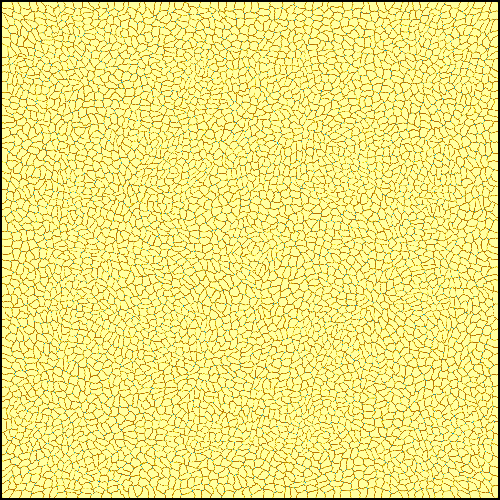
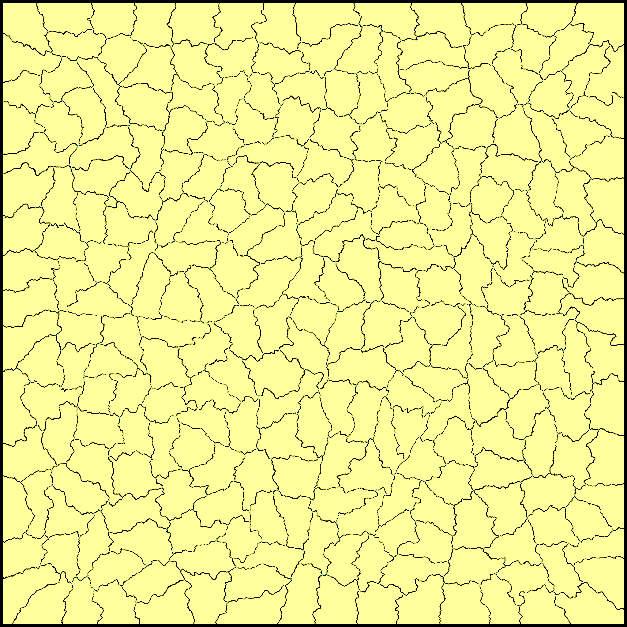
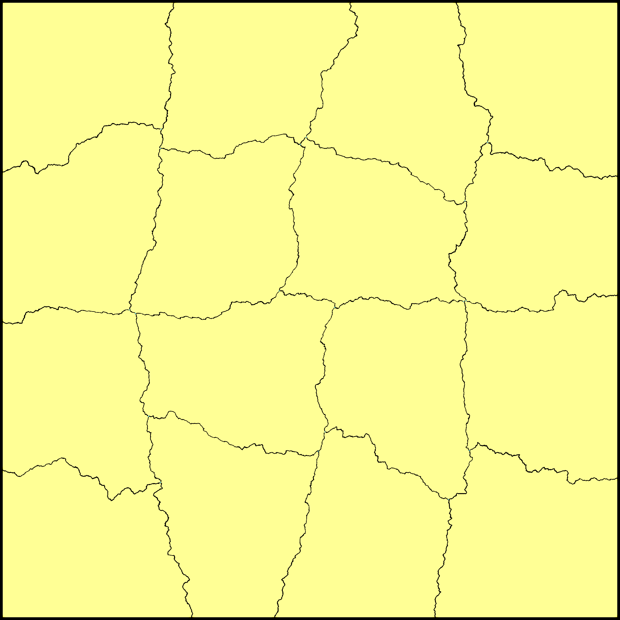
The construction of the subspaces is related to a hierarchical decomposition of the domain $\Omega$ into subdomains $\Omega_{l,i}$ for $0<l\leq L$ and $1\leq i\leq P_{l}$. “Hierarchical” means that each subdomain $\Omega_{l,i}$ is the union of subdomains on the next finer level $l+1$. In particular, our multilevel method employs a single fine mesh $\mathcal{T}_{h}$ given by the user. All subdomains are unions of elements of the mesh $\mathcal{T}_{h}$. Figure 1 shows a decomposition of a triangular mesh employing three levels.

The domain decomposition is obtained from a decomposition of $\mathcal{T}_{h}$ as follows:

  1. 1.

    On the finest level $L$, decompose $\mathcal{T}_{h}$ into $P_{L}$ overlapping sets

    $\displaystyle\mathcal{T}_{h,L,i}$ $\displaystyle\subset\mathcal{T}_{h},\quad 1\leq i\leq P_{L},$ $\displaystyle\bigcup_{i=1}^{P_{L}}\mathcal{T}_{h,L,i}$ $\displaystyle=\mathcal{T}_{h},$

    by first partitioning $\mathcal{T}_{h}$ into $P_{L}$ nonoverlapping sets of elements using a graph partitioner such es ParMetis [19] and then adding a user defined overlap $\delta$ in terms of layers of elements.

  2. 2.

    On levels $0<l<L$, determine decompositions of the subdomain index sets

    $\displaystyle J_{l,i}$ $\displaystyle\subset\{1,\ldots,P_{l+1}\},\quad 1\leq i\leq P_{l},$ $\displaystyle\bigcup_{i=1}^{P_{l}}J_{l,i}$ $\displaystyle=\{1,\ldots,P_{l+1}\}.$

    The sets $J_{l,i}$ may overlap but are not required to. Such decomposition is obtained by a graph partitioner using the subdomain graph instead of the mesh. With this we obtain the mesh partitioning on level $l$ as

    $$\mathcal{T}_{h,l,i}=\bigcup_{k\in J_{l,i}}\mathcal{T}_{h,l+1,k}.$$
  3. 3.

    The subdomains $\Omega_{l,i}$ are now defined from the mesh decomposition as

    $\displaystyle\Omega_{l,i}$ $\displaystyle=\text{Interior}\biggl{(}\bigcup_{\tau\in\mathcal{T}_{h,l,i}}\bar{\tau}\biggr{)},$ $\displaystyle 0<l\leq L,\quad 1\leq i\leq P_{l}.$
  4. 4.

    On the coarsest level 0 we employ always only one subdomain.

Refer to caption
Refer to caption
Refer to caption
Figure 1: Multilevel domain decomposition in two dimensions. A triangular mesh with 1.6 million vertices is partitioned into 4096 (level 3), 256 (level 2) and 16 (level 1) nested subdomains using ParMetis [19]. No overlap is used on the coarse levels.

For finite volume and discontinuous Galerkin methods we need to introduce notation for mesh faces. $\gamma$ is an interior face if it is the intersection of two elements $\tau^{-}(\gamma),\tau^{+}(\gamma)\in\mathcal{T}_{h}$ and has dimension $d-1$. All interior faces are collected in the set $\mathcal{F}_{h}^{I}$. Likewise, $\gamma$ is a boundary face if it is the intersection of some element $\tau^{-}(\gamma)\in\mathcal{T}_{h}$ with $\partial\Omega$ of dimension $d-1$. All boundary faces make up the set $\mathcal{F}_{h}^{\partial\Omega}$. With each $\gamma\in\mathcal{F}_{h}^{I}$ we associate a unit normal vector $\nu_{\gamma}$ oriented from $\tau^{-}(\gamma)$ to $\tau^{+}(\gamma)$. For a boundary face $\gamma\in\mathcal{F}_{h}^{\partial\Omega}$ its unit normal $\nu_{\gamma}$ coincides with the unit normal to $\partial\Omega$. Related to the submeshes $\mathcal{T}_{h,l,i}$ we define the corresponding sets of faces

(5a) $\displaystyle\mathcal{F}_{h,l,i}^{I}$ $\displaystyle=\{\gamma\in\mathcal{F}_{h}^{I}:\tau^{-}(\gamma)\in\mathcal{T}_{h,l,i}\wedge\tau^{+}(\gamma)\in\mathcal{T}_{h,l,i}\},$
(5b) $\displaystyle\mathcal{F}_{h,l,i}^{\partial\Omega}$ $\displaystyle=\{\gamma\in\mathcal{F}_{h}^{\partial\Omega}:\tau^{-}(\gamma)\in\mathcal{T}_{h,l,i}\}.$

2.3 Spectral Coarse Space Construction

Based on the hierarchical domain decomposition we can now formulate the construction of the coarse spaces $V_{h,l}\subseteq V_{h}$ and $V_{h,l,i}$ introduced in (4). First define the auxiliary local spaces

(6) $$\overline{V}_{h,l,i}=\{v|_{\Omega_{l,i}}:v\in V_{h,l}\}.$$

The restriction operator $r_{l,i}:V_{h,l}\to\overline{V}_{h,l,i}$, $r_{l,i}v=v|_{\Omega_{l,i}}$, restricts the domain of a finite element function. For $v$ being zero on $\partial\Omega_{l,i}\cap\Omega$, the extension operator $e_{l,i}:\overline{V}_{h,l,i}\to V_{h,l}$ extends functions by zero outside of $\Omega_{l,i}$. Another major ingredient is the partition of unity.

Definition 2.1.

A partition of unity on level $0<l\leq L$ is a family of operators $\chi_{l,i}:\overline{V}_{h,l,i}\to\overline{V}_{h,l,i}$ such that

  1. 1.

    $\chi_{l,i}v$ is zero on $\partial\Omega_{l,i}\cap\Omega$ for all $v\in\overline{V}_{h,l,i}$ and

  2. 2.

    $\sum_{i=1}^{P_{l}}e_{l,i}\chi_{l,i}r_{l,i}v=v$ for all $v\in V_{h,l}$,

Restriction and extension operators as well as the partition of unity operators with the required properties can be defined for conforming finite element spaces as well as discontinuous Galerkin finite element spaces.

The construction of the coarse spaces is now recursive over the levels:

  1. 1.

    Set $V_{h,L}=V_{h}$. Set $l=L$.

  2. 2.

    For each subdomain $1\leq i\leq P_{l}$ solve a GEVP

    (7) $$w_{l,i,k}\in\overline{V}_{l,i}:\qquad\overline{a}_{l,i}(w_{l,i,k},v)=\lambda_{l,i,k}\overline{b}_{l,i}(w_{l,i,k},v)\qquad\forall v\in\overline{V}_{l,i}$$

    with appropriately defined local bilinear forms $\overline{a}_{l,i}$ and $\overline{b}_{l,i}$ detailed below. Let eigenvalues and corresponding eigenvectors be ordered s.t. $\lambda_{l,i,k}\leq\lambda_{l,i,k+1}$.

  3. 3.

    With a user defined parameter $\eta$ define the coarse space $V_{h,l-1}$ as

    (8) $$V_{h,l-1}=\bigoplus_{i=1}^{P_{l}}\operatorname{span}\left\{\phi_{l,i,k}=e_{l,i}\chi_{l,i}w_{l,i,k}:\lambda_{l,i,k}<\eta\right\}.$$
  4. 4.

    Set $l=l-1$. If $l>0$ goto step 2, otherwise stop.

The subspaces for the subspace correction method based on $V_{h,l}$ are then given by

(9) $$V_{h,l,i}=\left\{v\in V_{h,l}:\operatorname{supp}v\subset\overline{\Omega}_{l,i}\right\}\subset\overline{V}_{h,l,i},\qquad 0<l\leq L,\quad 1\leq i\leq P_{l}$$

together with $V_{h,0}$.

Remark 2.2.

The most important properties of this construction are:

  • Within each level all GEVPs can be solved in parallel.

  • Basis functions $\phi_{l,i,k}\in V_{h}$ have support only in $\Omega_{l,i}$.

  • Functions in $V_{h,l,i}$ are zero at their subdomain boundary (except on the global Neumann boundary). Functions in $\overline{V}_{h,l,i}$ are not necessarily zero at their subdomain boundary (except on the global Dirichlet boundary).

3 Convergence Theory

3.1 Standard Subspace Correction Theory

For the standard analysis of subspace correction methods, the following $a_{h}$-orthogonal projections $\mathcal{P}_{l}:V_{h}\to V_{h,l}$ and $\mathcal{P}_{l,i}:V_{h}\to V_{h,l,i}$ are introduced [32, 30]:

$\displaystyle a_{h}(\mathcal{P}_{l}w,v)$ $\displaystyle=a_{h}(w,v),\quad\forall v\in V_{h,l},$ $\displaystyle a_{h}(\mathcal{P}_{l,i}w,v)$ $\displaystyle=a_{h}(w,v),\quad\forall v\in V_{h,l,i}.$

This allows to write the error propagation operator $\mathcal{E}$ of the iteration (3) as

$\displaystyle\mathcal{E}$ $\displaystyle=\mathcal{I}-\omega\mathcal{P},$ $\displaystyle\mathcal{P}=\mathcal{P}_{0}+\sum_{l=1}^{L}\sum_{i=1}^{P_{l}}\mathcal{P}_{l,i}.$

Taking $\omega=1/\lambda_{\max}(\mathcal{P})$, the convergence factor of the iteration (3) is $\rho=1-1/\kappa_{2}(\mathcal{P})$ with the spectral condition number $\kappa_{2}(\mathcal{P})=\lambda_{\max}(\mathcal{P})/\lambda_{\min}(\mathcal{P})$. The goal of the analysis below is to provide upper and lower bounds of the form

$$\gamma a_{h}(v,v)\leq a_{h}(\mathcal{P}v,v)\leq\Gamma a_{h}(v,v)\qquad\forall v\in V_{h},$$

which in turn give a bound on the condition number $\kappa_{2}(\mathcal{P})\leq\Gamma/\gamma$.

The analysis is based on two major properties.

Definition 3.1 (Coloring and domain decomposition).
  1. 1.

    We say the multilevel domain decomposition admits a level-wise coloring with $k_{0}\in\mathbb{N}$ colors, if for each level $0<l\leq L$ there exists a map $c_{l}:\{1,\ldots,P_{l}\}\to\{1,\ldots,k_{0}\}$ such that

    $$i\neq j\wedge c_{l}(i)=c_{l}(j)\Rightarrow a_{h}(v_{i},v_{j})=0\qquad\forall v_{i}\in V_{h,l,i},v_{j}\in V_{h,l,j}.$$
  2. 2.

    The multilevel domain decomposition is called admissible, if on each level $0<l\leq L$ every interior face $\gamma$ is interior to at least one subdomain.

Lemma 3.2.

Let the multilevel domain decomposition have a finite coloring with $k_{0}$ colors. Then parallel subspace correction satisfies the upper bound

$$a_{h}(\mathcal{P}v,v)\leq(1+k_{0}L)a_{h}(v,v)\qquad\forall v\in V_{h}.$$
Proof 3.3.

See [28, p. 182].

Definition 3.4 (Stable splitting).

The subspaces $V_{h,0}$ and $V_{h,l,i}$, $0<l\leq L$, $1\leq i\leq P_{l}$, admit a stable splitting if there exists $C_{0}>0$ and for each $v\in V_{h}$ a decomposition $v=v_{0}+\sum_{i=1}^{L}\sum_{i=1}^{P_{l}}v_{l,i}$, $v_{0}\in V_{h,0}$, $v_{l,i}\in V_{h,l,i}$, such that

$$a_{h}(v_{0},v_{0})+\sum_{i=1}^{L}\sum_{i=1}^{P_{l}}a_{h}(v_{l,i},v_{l,i})\leq C_{0}\,a_{h}(v,v).$$

Lemma 3.5.

If the subspaces $V_{h,0}$ and $V_{h,l,i}$, $0<l\leq L$, $1\leq i\leq P_{l}$ admit a stable splitting with constant $C_{0}$, parallel subspace correction satisfies the lower bound

$$C_{0}^{-1}a_{h}(v,v)\leq a_{h}(\mathcal{P}v,v)\qquad\forall v\in V_{h}.$$
Proof 3.6.

See e.g. [30].

Theorem 3.7.

If the subspaces $V_{h,0}$ and $V_{h,l,i}$, $0<l\leq L$, $1\leq i\leq P_{l}$ have a finite coloring with $k_{0}$ colors and admit a stable splitting with constant $C_{0}$, parallel subspace correction satisfies the bound

$$\kappa_{2}(\mathcal{P})\leq C_{0}(1+k_{0}L).$$
Proof 3.8.

Follows immediately from Lemma 3.2 and Lemma 3.5.

3.2 Abstract Schwarz Theory for Spectral Domain Decomposition

We now generalize the theory in [29] to the multilevel case and to more general discretization schemes. For each application, the following three definitions have to be verified.

Definition 3.9 (Strengthened triangle inequality under the square).

The domain decomposition allows a strengthened triangle inequality under the square if there exists $a_{0}>0$ independent of $0<l\leq L$ and $P_{l}$ such that for any collection of $v_{l,i}\in V_{h,l,i}$:

$$\left\|\sum_{i=1}^{P_{l}}v_{l,i}\right\|_{a_{h}}^{2}\leq a_{0}\sum_{i=1}^{P_{l}}\left\|v_{l,i}\right\|_{a_{h}}^{2}.$$

Here $\|v\|_{a_{h}}=\sqrt{a_{h}(v,v)}$ is the norm induced by $a_{h}$.

Definition 3.10 (Positive semi-definite splitting).

The bilinear forms $\overline{a}_{l,i}$ introduced in (7) provide a positive semi-definite splitting of $a_{h}$ if there exists $b_{0}>0$ independent of $0<l\leq L$ and $P_{l}$ such that for each level $0<l\leq L$:

$$\sum_{i=1}^{P_{l}}\left|r_{l,i}v_{l}\right|_{\overline{a}_{l,i}}^{2}\leq b_{0}\left\|v_{l}\right\|_{a_{h}}^{2},\qquad\forall v_{l}\in V_{h,l}.$$

Here $|v|_{\overline{a}_{l,i}}=\sqrt{\overline{a}_{l,i}(v,v)}$ is the semi-norm induced by $\overline{a}_{l,i}$. Symmetric positive semi-definite splittings on the algebraic level were introduced in [2, 3].

Definition 3.11 (Local stability).

The subspaces $V_{h,l}$ and $V_{h,l,i}$ are called locally stable if there exists a constant $C_{1}>0$ idependent of $l$ and for each $v_{l}\in V_{h,l}$, $1\leq l\leq L$, a decomposition $v_{l}=v_{l-1}+\sum_{i=1}^{P_{l}}v_{l,i}$ with $v_{l-1}\in V_{h,l-1}$ and $v_{l,i}\in V_{h,l,i}$ such that the following inequalities hold:

$$\left\|v_{l,i}\right\|_{a_{h}}^{2}\leq C_{1}\left|r_{l,i}v_{l}\right|_{\overline{a}_{l,i}}^{2},\qquad 1\leq i\leq P_{l}.$$

Lemma 3.12 (Levelwise stability).

Let the spectral coarse spaces admit strengthened triangle inequalities under the square, let the bilinear forms $\overline{a}_{l,i}$ provide a symmetric positive semi-definite splitting and let the subspaces $V_{h,l,i}$ be locally stable. Then, for each level $0<l\leq L$ there exists a decomposition $v_{l}=v_{l-1}+\sum_{i=1}^{P_{l}}v_{l,i}$ with $v_{l-1}\in V_{h,l-1}$ and $v_{l,i}\in V_{h,l,i}$ such that

$\displaystyle\left\|v_{l-1}\right\|_{a_{h}}^{2}\leq 2(1+a_{0}b_{0}C_{1})\left\|v_{l}\right\|_{a_{h}}^{2}$

and

$\displaystyle\left\|v_{l-1}\right\|_{a_{h}}^{2}+\sum_{i=1}^{P_{l}}\left\|v_{l,i}\right\|_{a_{h}}^{2}\leq(2+b_{0}C_{1}(1+2a_{0}))\left\|v_{l}\right\|_{a_{h}}^{2}.$
Proof 3.13.

Adaptation of [29, Lemma 2.9]. From Def. 3.11 and Def. 3.10 we get

$\displaystyle\sum_{i=1}^{P_{l}}\left\|v_{l,i}\right\|_{a_{h}}^{2}\leq C_{1}\sum_{i=1}^{Pl}\left|r_{l,i}v_{l}\right|_{\overline{a}_{l,i}}^{2}\leq b_{0}C_{1}\left\|v_{l}\right\|_{a_{h}}^{2}.$

Thus, it follows from $v_{l-1}=v_{l}-\sum_{i=1}^{P_{l}}v_{l,i}$ and from Def. 3.9 that

$\displaystyle\left\|v_{l-1}\right\|_{a_{h}}^{2}$ $\displaystyle=\left\|v_{l}-\sum_{i=1}^{P_{l}}v_{l,i}\right\|_{a_{h}}^{2}\leq 2\left\|v_{l}\right\|_{a_{h}}^{2}+2\left\|\sum_{i=1}^{P_{l}}v_{l,i}\right\|_{a_{h}}^{2}\leq 2\left\|v_{l}\right\|_{a_{h}}^{2}+2a_{0}\sum_{i=1}^{P_{l}}\left\|v_{l,i}\right\|_{a_{h}}^{2}$
$\displaystyle\leq 2\left\|v_{l}\right\|_{a_{h}}^{2}+2a_{0}b_{0}C_{1}\left\|v_{l}\right\|_{a_{h}}^{2}=2(1+a_{0}b_{0}C_{1})\left\|v_{l}\right\|_{a_{h}}^{2}.$

Combining both results yields

$\displaystyle\left\|v_{l-1}\right\|_{a_{h}}^{2}+\sum_{i=1}^{P_{l}}\left\|v_{l,i}\right\|_{a_{h}}^{2}$ $\displaystyle\leq(2+b_{0}C_{1}(1+2a_{0}))\left\|v_{l}\right\|_{a_{h}}^{2}.$

The two-level decomposition from Definition 3.11 implies a multilevel decomposition as follows: For any given function $v_{h}\in V_{h}$:

(10) $$V_{h}\ni v_{h}=v_{L}=v_{0}+\sum_{l=1}^{L}\sum_{i=1}^{P_{l}}v_{l,i},\qquad\text{with}\qquad v_{l}-v_{l-1}=\sum_{i=1}^{P_{l}}v_{l,i}.$$

We can now formulate the first major result of our paper.

Lemma 3.14 (Multilevel stability).

Let the spectral coarse spaces admit strengthened triangle inequalities under the square, let the bilinear forms $\overline{a}_{l,i}$ provide a symmetric positive semi-definite splitting and let the subspaces $V_{h,l,i}$ be locally stable. Then the multilevel decomposition (10) satisfies for any $v_{h}\in V_{h}$

$$\|v_{0}\|_{a_{h}}^{2}+\sum_{l=1}^{L}\sum_{i=1}^{P_{l}}\left\|v_{l,i}\right\|_{a_{h}}^{2}\leq C^{L}\left(1+\frac{b_{0}C_{1}}{C-1}\right)\|v_{h}\|_{a_{h}}^{2}$$

with $C=2(1+a_{0}b_{0}C_{1})$.

Proof 3.15.

For any level $0<l\leq L$, we obtain as in the proof of Lemma 3.12

$\displaystyle\sum_{i=1}^{P_{l}}\left\|v_{l,i}\right\|_{a_{h}}^{2}\leq C_{1}\sum_{i=1}^{P_{l}}\left|r_{l,i}v_{l}\right|_{\overline{a}_{l,i}}^{2}\leq b_{0}C_{1}\left\|v_{l}\right\|_{a_{h}}^{2}.$

Furthermore, Lemma 3.12 implies

$\displaystyle\|v_{l}\|_{a_{h}}^{2}\leq\left[2(1+a_{0}b_{0}C_{1})\right]^{L-l}\|v_{h}\|_{a_{h}}^{2}$

for $0\leq l\leq L$. Together we obtain with setting $C=2(1+a_{0}b_{0}C_{1})$

$\displaystyle\|v_{0}\|_{a_{h}}^{2}$ $\displaystyle+\sum_{l=1}^{L}\sum_{i=1}^{P_{l}}\left\|v_{l,i}\right\|_{a_{h}}^{2}\leq C^{L}\|v_{h}\|_{a_{h}}^{2}+b_{0}C_{1}\|v_{h}\|_{a_{h}}^{2}\sum_{l=1}^{L}C^{L-l}$
$\displaystyle\leq C^{L}\|v_{h}\|_{a_{h}}^{2}+b_{0}C_{1}\frac{C^{L}}{C-1}\|v_{h}\|_{a_{h}}^{2}=C^{L}\left(1+\frac{b_{0}C_{1}}{C-1}\right)\|v_{h}\|_{a_{h}}^{2}.$

Theorem 3.16.

Let the assumptions of Lemma 3.14 hold and let the domain decomposition admit a coloring with $k_{0}$ colors on each level. Then the parallel multilevel subspace correction method satisfies the condition number bound

$$\kappa_{2}(\mathcal{P})\leq C^{L}\left(1+\frac{b_{0}C_{1}}{C-1}\right)(1+k_{0}L).$$

with $C=2(1+a_{0}b_{0}C_{1})$.

Proof 3.17.

Follows from Lemma 3.14 and Theorem 3.7.

Remark 3.18.

The upper bound in Lemma 3.12 predicts an exponential increase of the condition number with the number of levels $L+1$. Since we are only interested in a moderate number of levels $L+1=3$ or $4$, this may be acceptable. Moreover, our numerical results below suggest that the bound is pessimistic. In our experiments, we observe $\kappa_{2}(\mathcal{P})=O(L)$, which may actually be due to the lower bound.

3.3 Generalized Eigenproblems

The stability estimates in Definition 3.11 are closely linked to properties of the GEVP solved in each subdomain. This subsection establishes the necessary results. In this section, $a:V\times V\to\mathbb{R}$ and $b:V\times V\to\mathbb{R}$ denote generic symmetric and positive semi-definite bilinear forms on a $n$-dimensional vector space $V$. For a symmetric and positive semi-definite bilinear form $a$ denote by

$$\ker a=\{v\in V\,:\,a(v,w)=0\ \forall w\in V\}$$

the kernel of $a$. In the following, we make the important assumption (to be verified below for the bilinear forms in (7)) that the bilinear forms satisfy

(11) $$\ker a\cap\ker b=\{0\}.$$
Definition 3.19 (Generalized Eigenvalue Problem).

We call $(\lambda,p)\in\mathbb{R}\cup\{\infty\}\times V$ with $p\neq 0$, an eigenpair of $(a,b)$, if either $p\notin\ker b$ and

(12) $\displaystyle a(p,v)=\lambda b(p,v)\qquad\forall v\in V$

or $p\in\ker b$ and $\lambda=\infty$. For such a pair, $\lambda$ is called an eigenvalue and $p$ an eigenvector of $(a,b)$. The collection of all eigenvalues (counted according to their geometric multiplicity) is called the spectrum of $(a,b)$.

Lemma 3.20.

The generalized eigenvalue problem (12) is non-defective, i.e. it has a full set of eigenvectors with either $0\leq\lambda\in\mathbb{R}$ or $\lambda=+\infty$.

Proof 3.21.

Assumption (11) implies that $a+b$ is a symmetric and positive definite bilinear form. Employing a spectral transformation yields

$\displaystyle a(p,v)=\lambda b(p,v)\quad\Leftrightarrow\quad b(p,v)=\mu(a+b)(p,v)\quad\forall v\in V,\qquad\mu=\frac{1}{1+\lambda},$

with a symmetric and positive definite bilinear form on the right. Now standard spectral theory for this problem shows that there exists a full set of eigenvectors with real nonnegative eigenvalues. It also follows that $\mu\leq 1$. Now $\mu=0$ corresponds to $\lambda=+\infty$, $p\in\ker b$ and $\mu=1$ corresponds to $\lambda=0$, $p\in\ker a$.

From now on we assume that eigenpairs $(\lambda_{k},p_{k})$ are ordered by size, i.e. $\lambda_{k}\leq\lambda_{k+1}$. With $r=\dim\ker a$ and $s=\dim\ker b$ the spectrum reads

$$0=\lambda_{1}=\ldots=\lambda_{r}<\lambda_{r+1}\leq\ldots\leq\lambda_{n-s}<\lambda_{n-s+1}=\ldots=\lambda_{n}=+\infty.$$

The eigenvectors $p_{1},\ldots,p_{n-s}$, corresponding to the first $n-s$ eigenvalues, can be chosen to be simultaneously $b$-orthonormal and $a$-orthogonal. The remaining eigenvectors $p_{n-s+1},\ldots,p_{n}\in\ker b$ are chosen to be $a$-orthogonal and are also $b$-orthogonal, such that $\{p_{1},\ldots,p_{n}\}$ forms a basis of $V$.

The projection $\Pi_{m}:V\to V$ to the first $m\leq n-s$ eigenvectors is defined by

(13) $$\Pi_{m}v:=\sum_{k=1}^{m}b(v,p_{k})p_{k}\,.$$

Furthermore, we also introduce the induced semi-norms

$\displaystyle|v|_{a}$ $\displaystyle=\sqrt{a(v,v)},$ $\displaystyle|v|_{b}$ $\displaystyle=\sqrt{b(v,v)}.$
Lemma 3.22.

Let $a,b$ be positive semi-definite bilinear forms on $V$ with $\ker a\cap\ker b=\{0\}$ and $(\lambda_{k},p_{k})$, $k=1,\ldots,n$, eigenpairs of (12) with $p_{k}$, $k\leq n-s$, $b$-orthonormal and $p_{k}$, $k>n-s$, $a$-orthogonal. Then the projection $\Pi_{m}$ satisfies the stability estimates

(14) $$|\Pi_{m}v|_{a}\leq|v|_{a}\qquad\text{and}\qquad|v-\Pi_{m}v|_{a}\leq|v|_{a},\qquad\forall v\in V$$

and for $m\geq r$

(15) $$|v-\Pi_{m}v|_{b}^{2}\leq\frac{1}{\lambda_{m+1}}|v-\Pi_{m}v|_{a}^{2},\qquad\forall v\in V.$$
Proof 3.23.

The case $\ker b=\{0\}$ is proved in [29, Lemma 2.11]. The proof of (14) in [29] extends without any modification to the case $\ker b\neq\{0\}$, since the $p_{k}$ are still $a$-orthogonal and $m\leq n-s$. For the proof of (15) a small modification is necessary. Let $v=\sum_{k=1}^{n}\alpha_{k}p_{k}$ be arbitrary. Then,

$\displaystyle|v-\Pi_{m}v|_{b}^{2}$ $\displaystyle=b\left(\sum_{k=m+1}^{n}\alpha_{k}p_{k},\sum_{k=m+1}^{n}\alpha_{k}p_{k}\right)=\sum_{k=m+1}^{n-s}\alpha_{k}^{2}=\sum_{k=m+1}^{n-s}\alpha_{k}^{2}\frac{a(p_{k},p_{k})}{\lambda_{k}}$
$\displaystyle\leq\frac{1}{\lambda_{m+1}}\sum_{k=m+1}^{n-s}\alpha_{k}^{2}a(p_{k},p_{k})\leq\frac{1}{\lambda_{m+1}}\sum_{k=m+1}^{n}\alpha_{k}^{2}a(p_{k},p_{k})$
$\displaystyle=\frac{1}{\lambda_{m+1}}a\left(v-\Pi_{m}v,v-\Pi_{m}v\right)=\frac{1}{\lambda_{m+1}}|v-\Pi_{m}v|_{a}^{2}.$

Remark 3.24.

In [29] the bilinear form $b$ in the GenEO method is positive semi-definite but the authors did not include this case in their Lemma 2.11 but rather treat this fact in Lemmata 3.11, 3.16 and 3.18 for a special case. We think the assumption $\ker a\cap\ker b=\{0\}$ is more natural and easy to prove in applications. In [3, Lemma 2.3] the authors consider the GEVP for two symmetric positive semi-definite matrices $A$, $B$ with nontrivial intersection $\ker A\cap\ker B\neq\{0\}$. This is not required in our analysis in the variational setting. However, in the implementation a basis for the space $V=V_{l}$ is required on each level. It turns out, it is prohibitively expensive to construct such a basis on levels $l<L$ and only a generating system is available. This then results in a GEVP with $\ker A\cap\ker B\neq\{0\}$. We refer to Section 4.2 how to overcome this problem.

3.4 Application to Continuous Galerkin

In this section, we consider the application to the solution of the scalar elliptic boundary value problem

(16a) $\displaystyle-\nabla\cdot(K\nabla u)$ $\displaystyle=f$ $\displaystyle\text{in $\Omega$},$
(16b) $\displaystyle u$ $\displaystyle=0$ $\displaystyle\text{on $\Gamma_{D}\subseteq\partial\Omega$},$
(16c) $\displaystyle-(K\nabla u)\cdot\nu$ $\displaystyle=\psi$ on $\Gamma_{N}=\partial\Omega\setminus\Gamma_{D}$

with Dirichlet and Neumann boundary conditions in a domain $\Omega\subset\mathbb{R}^{d}$. The diffusion coefficient $K(x)\in\mathbb{R}^{d\times d}$ is symmetric and positive definite with eigenvalues bounded uniformly from above and below for all $x\in\Omega$.

We discretize (16) with conforming finite elements on simplicial or hexahedral meshes [14] resulting in the weak formulation

$$u_{h}\in V_{h}:\qquad a_{h}(u,v)=l(v)\qquad\forall v\in V_{h}$$

with

$\displaystyle a_{h}(u,v)$ $\displaystyle=\sum_{\tau\in\mathcal{T}_{h}}a_{\tau}(u,v),$ $\displaystyle a_{\tau}(u,v)$ $\displaystyle=\int\limits_{\tau}(K\nabla u)\cdot\nabla v\,dx,$ $\displaystyle l(v)=\int\limits_{\Omega}fv\,dx-\int\limits_{\Gamma_{N}}\psi v\,ds.$

The local bilinear forms $\overline{a}_{l,i}$ on the left side of the GEVP (7) are then defined as

(17) $$\overline{a}_{l,i}(u,v)=\sum_{\tau\in\mathcal{T}_{h,l,i}}a_{\tau}(u,v).$$

The following Lemma shows that the $\overline{a}_{l,i}$ define a symmetric positive semi-definite splitting and the strengthened triangle inequality under the square holds.

Lemma 3.25.

Let the domain decomposition satisfy definition 3.1 with $k_{0}$. Then the local bilinear forms (17) satisfy definitions 3.9 and 3.10 with $a_{0}=b_{0}=k_{0}$.

Proof 3.26.

Follows from any $\tau\in\mathcal{T}_{h}$ being in at most $k_{0}$ subdomains on any level $l$.

Extending the results in [29], we show local stability (Def. 3.11) for three different right hand sides in the GEVPs:

(18a) $\displaystyle\overline{b}_{l,i}^{\text{1}}(u,v)$ $\displaystyle=\overline{a}_{l,i}\left(\chi_{l,i}u,\chi_{l,i}v\right)=a\left(e_{l,i}\chi_{l,i}u,e_{l,i}\chi_{l,i}v\right),$
(18b) $\displaystyle\overline{b}_{l,i}^{\text{2}}(u,v)$ $\displaystyle=\mathring{a}_{l,i}\left(\chi_{l,i}u,\chi_{l,i}v\right),$
(18c) $\displaystyle\overline{b}_{l,i}^{\text{3}}(u,v)$ $\displaystyle=\overline{a}_{l,i}\left(u-\chi_{l,i}u,v-\chi_{l,i}v\right),$

where

$$\mathring{a}_{l,i}(u,v)=\sum_{\tau\in\mathring{\mathcal{T}}_{h,l,i}}a_{\tau}(u,v)\quad\text{and}\quad\mathring{\mathcal{T}}_{h,l,i}=\left\{\tau\in\mathcal{T}_{h,l,i}:\tau\in\mathcal{T}_{h,l,j}\text{ for some }j\neq i\right\}.$$

The choice (18b) defines the original GenEO method from [29]. The other two choices are easier to apply on the coarse levels $l<L$ and for discontinuous Galerkin (below).

Lemma 3.27.

The bilinear forms $\overline{b}_{l,i}^{\alpha}$, $\alpha=1,2,3$, satisfy $\ker\overline{a}_{l,i}\cap\ker\overline{b}_{l,i}^{\alpha}=\{0\}$.

Proof 3.28.

For subdomains touching the Dirichlet boundary, $\overline{a}_{l,i}$ is positive definite, so $\ker\overline{a}_{l,i}=\{0\}$. For subdomains not touching the Dirichlet boundary, $\ker\overline{a}_{l,i}=\operatorname{span}\{c\}$, where $c\equiv 1$ is the constant one function. Now $\chi_{l,i}c$ and $(1-\chi_{l,i})c$ are not in $\ker\overline{a}_{l,i}$ Moreover, $\chi_{l,i}c$ is also not in $\ker\mathring{a}_{l,i}$.

Each choice of $\overline{b}_{l,i}^{\alpha}$, $\alpha=1,2,3$, gives rise to a projection operator $\Pi^{\alpha}_{l,i,m}$, as defined in (13), onto the eigenvectors corresponding to the smallest $m$ eigenvalues in subdomain $i$ on level $l$. Typically, for some threshold $\eta>0$, we will choose $m=m(\eta)$ such that $\lambda_{l,i,k}\leq\eta$ for all $k\leq m(\eta)$. Making use of these projection operators, the stable two-level splitting in Definition 3.11, for a level $l$ function $v_{l}\in V_{h,l}$, can be achieved by choosing

(19) $\displaystyle v_{l,i}$ $\displaystyle=\chi_{l,i}(I-\Pi^{\alpha}_{l,i,m(\eta)})r_{l,i}v_{l},$ $\displaystyle v_{l-1}$ $\displaystyle=\sum_{i=1}^{P_{l}}\chi_{l,i}\Pi^{\alpha}_{l,i,m(\eta)}r_{l,i}v_{l}.$

Now we can state the main result of this subsection.

Lemma 3.29.

For $\alpha=1,2,3$, the splittings (19) using the projections $\Pi^{\alpha}_{l,i,m(\eta)}$ to the first $m(\eta)$ eigenvectors are locally stable with constants $C_{1}^{\alpha}$ given by

$\displaystyle C_{1}^{1}$ $\displaystyle=\eta^{-1},$ $\displaystyle C_{1}^{2}$ $\displaystyle=1+\eta^{-1},$ $\displaystyle C_{1}^{3}$ $\displaystyle=2\left(1+\eta^{-1}\right).$
Proof 3.30.

All three cases follow from Lemma 3.22. In the case $\alpha=1$, we obtain

$\displaystyle\left\|v_{l,i}\right\|_{a_{h}}^{2}$ $\displaystyle=\left\|\chi_{l,i}(I-\Pi^{1}_{l,i,m(\eta)})r_{l,i}v_{l}\right\|_{a_{h}}^{2}=\left\|(I-\Pi^{1}_{l,i,m(\eta)})r_{l,i}v_{l}\right\|_{\overline{b}^{1}_{l,i}}^{2}$
$\displaystyle\leq\eta^{-1}\left\|(I-\Pi^{1}_{l,i,m(\eta)})r_{l,i}v_{l}\right\|_{\overline{a}_{l,i}}^{2}\leq\eta^{-1}\left\|r_{l,i}v_{l}\right\|_{\overline{a}_{l,i}}^{2}.$

For $\alpha=2$, observe first that $(\chi_{l,i}v)|_{\tau}=v|_{\tau}$ , for all elements $\tau\in\mathcal{T}_{h,l,i}\setminus\mathring{\mathcal{T}}_{h,l,i}$. Thus,

$\displaystyle\bigl{\|}v_{l,i}$ $\displaystyle\bigr{\|}_{a_{h}}^{2}=\sum_{\tau\in\mathring{\mathcal{T}}_{h,l,i}}a_{\tau}\left(v_{l,i},v_{l,i}\right)+\sum_{\tau\in\mathcal{T}_{h,l,i}\setminus\mathring{\mathcal{T}}_{h,l,i}}a_{\tau}\left(v_{l,i},v_{l,i}\right)$
$\displaystyle\leq\left|(I-\Pi^{2}_{l,i,m(\eta)})r_{l,i}v_{l}\right|_{\overline{b}_{l,i}}^{2}+\left|(I-\Pi^{2}_{l,i,m(\eta)})r_{l,i}v_{l}\right|_{\overline{a}_{l,i}}^{2}$
$\displaystyle\leq\Big{(}\eta^{-1}+1\Big{)}\left|(I-\Pi^{2}_{l,i,m(\eta)})r_{l,i}v_{l}\right|_{\overline{a}_{l,i}}^{2}\leq\left(1+\eta^{-1}\right)\left|r_{l,i}v_{l}\right|_{\overline{a}_{l,i}}^{2}.$

Finally, consider $\alpha=3$: Since $v_{l,i}$ is zero on $\partial\Omega_{l,i}$ ,

$\displaystyle\left\|v_{l,i}\right\|_{a_{h}}^{2}$ $\displaystyle=\left|\chi_{l,i}(I-\Pi^{3}_{l,i,m(\eta)})r_{l,i}v_{l}\right|_{\overline{a}_{l,i}}^{2}$
$\displaystyle=\left|(I-\Pi^{3}_{l,i,m(\eta)})r_{l,i}v_{l}-(I-\chi_{l,i})(I-\Pi^{3}_{l,i,m(\eta)})r_{l,i}v_{l}\right|_{\overline{a}_{l,i}}^{2}$
$\displaystyle\leq 2\left|(I-\Pi^{3}_{l,i,m(\eta)})r_{l,i}v_{l}\right|_{\overline{a}_{l,i}}^{2}+2\left|(I-\Pi^{3}_{l,i,m(\eta)})r_{l,i}v_{l}\right|_{\overline{b}_{l,i}}^{2}$
$\displaystyle\leq 2(1+\eta^{-1})\left|(I-\Pi^{3}_{l,i,m(\eta)})r_{l,i}v_{l}\right|_{\overline{a}_{l,i}}^{2}\leq 2(1+\eta^{-1})\left|r_{l,i}v_{l}\right|_{\overline{a}_{l,i}}^{2}.$

3.5 Application to Discontinuous Galerkin

Here we consider the weighted symmetric interior penalty (WSIP) discontinuous Galerkin (DG) method from [15] for the problem (18). The DG finite element space of degree $k$ on the mesh $\mathcal{T}_{h}$ is

(20) $$V_{h}^{\text{DG}}=\{v\in L_{2}(\Omega):v|_{\tau}=p_{\tau}\circ\mu_{\tau}^{-1},p_{\tau}\in\mathbb{P}_{k}\}$$

where $\mathbb{P}_{k}$ is either the set of polynomials of total degree $k$ for simplices or the set of polynomials of maximum degree $k$ for cuboid elements. A function $v\in V_{h}^{\text{DG}}$ is two-valued on an interior face $\gamma\in\mathcal{F}_{h}^{I}$ and by $v^{-}$ we denote the restriction to $\gamma$ from $\tau^{-}(\gamma)$ and by $v^{+}$ the restriction from $\tau^{+}(\gamma)$. For any point $x\in\gamma\in\mathcal{F}_{h}^{I}$ we define the jump and the weighted average

$\displaystyle\llbracket v\rrbracket(x)$ $\displaystyle=v^{-}(x)-v^{+}(x),$ $\displaystyle\{v\}_{\omega}(x)$ $\displaystyle=\omega^{-}v^{-}(x)-\omega^{+}v^{+}(x)$

for some weights $\omega^{-}+\omega^{+}=1$, $\omega^{\pm}\geq 0$. A particular choice of the weights depending on the absolute permeability tensor $K$ has been introduced in [15]. Assuming that $K^{\pm}$ is constant on $\tau^{\pm}(\gamma)$, they set $\omega^{-}=\delta_{K\nu}^{+}/(\delta_{K\nu}^{-}+\delta_{K\nu}^{+})$ and $\omega^{+}=\delta_{K\nu}^{-}/(\delta_{K\nu}^{-}+\delta_{K\nu}^{+})$ for $\delta_{K\nu}^{\pm}=\nu_{\gamma}^{T}K^{\pm}\nu_{\gamma}$. Finally, for any domain $Q\subset\Omega$ we set

$$(v,w)_{0,Q}=\int_{Q}vw\ dx,\qquad\|v\|_{0,Q}=\sqrt{(v,v)_{0,Q}}.$$

The WSIP-DG method [15] for numerically solving (16) now reads

(21) $$u_{h}\in V_{h}^{\text{DG}}\quad:\quad a_{h}^{\text{DG}}(u_{h},v)=l_{h}^{\text{DG}}(v)\qquad\forall v\in V_{h}^{\text{DG}},$$

where

(22) $$a_{h}^{\text{DG}}(u,v)=\sum_{\tau\in\mathcal{T}_{h}}a_{\tau}(u,v)+\sum_{\gamma\in\mathcal{F}_{h}^{I}}a^{I}_{\gamma}(u,v)+\sum_{\gamma\in\mathcal{F}_{h}^{D}}a^{D}_{\gamma}(u,v)$$

with $\mathcal{F}_{h}^{D}\subseteq\mathcal{F}_{h}^{\partial\Omega}$ denoting faces on $\Gamma_{D}$ and where

$\displaystyle a^{I}_{\gamma}(u,v)$ $\displaystyle=\sigma_{\gamma}(\llbracket u\rrbracket,\llbracket v\rrbracket)_{0,\gamma}-(\{K\nabla u\}_{\omega}\cdot\nu_{\gamma},\llbracket v\rrbracket)_{0,\gamma}-(\{K\nabla v\}_{\omega}\cdot\nu_{\gamma},\llbracket u\rrbracket)_{0,\gamma},$
$\displaystyle a^{D}_{\gamma}(u,v)$ $\displaystyle=\sigma_{\gamma}(u,v)_{0,\gamma}-((K\nabla u)\cdot\nu_{\gamma},v)_{0,\gamma}-((K\nabla v)\cdot\nu_{\gamma},u)_{0,\gamma},$
$\displaystyle l^{\text{DG}}(v)$ $\displaystyle=\sum_{\tau\in\mathcal{T}_{h}}(f,v)_{0,\tau}-\sum_{\gamma\in\mathcal{F}_{h}^{N}}(\psi,v)_{0,\gamma}-\sum_{\gamma\in\mathcal{F}_{h}^{D}}\Bigl{[}((K\nabla v)\cdot\nu_{\gamma},g)_{0,\gamma}-\sigma_{\gamma}(g,v)_{0,\gamma}\Bigr{]}.$

For each face (interior or boundary), $\sigma_{\gamma}>0$ defines a penalty parameter to be chosen and specified below. The bilinear form $a_{h}^{\text{DG}}$ is symmetric and positive definite, provided the penalty parameters $\sigma_{\gamma}$ are chosen large enough [15].

We now prepare some results necessary for proving the requirements stated in Definitions 3.9 and 3.10.

Lemma 3.31.

Let $K(x)$ be a diffusion coefficient, constant on each element, and choose $s\in\mathbb{R}$, $s>0$ an arbitrary number. Then the following estimates hold:

$\displaystyle\Bigl{|}2((K\nabla v)\cdot\nu_{\gamma},v)_{0,\gamma}\Bigr{|}$ $\displaystyle\leq\frac{1}{s}a_{\tau^{-}(\gamma)}(v,v)+\theta_{\gamma}\|v\|_{0,\gamma}^{2},$ $\displaystyle\gamma\in\mathcal{F}_{h}^{D},$
$\displaystyle\Bigl{|}2(\{K\nabla v\}_{\omega}\cdot\nu_{\gamma},\llbracket v\rrbracket)_{0,\gamma}\Bigr{|}$ $\displaystyle\leq\frac{1}{s}(a_{\tau^{-}(\gamma)}(v,v)+a_{\tau^{+}(\gamma)}(v,v))+\theta_{\gamma}\|\llbracket v\rrbracket\|_{0,\gamma}^{2},$ $\displaystyle\gamma\in\mathcal{F}_{h}^{I},$

with

$$\theta_{\gamma}(s)=\begin{cases}\displaystyle\frac{C_{t}^{2}s\delta_{K\nu}}{2h_{\tau}}&\gamma\in\mathcal{F}_{h}^{D}\\ \displaystyle\frac{C_{t}^{2}s}{\min(h_{\tau^{-}},h_{\tau^{+}})}\frac{\delta_{K\nu}^{-}\delta_{K\nu}^{+}}{\delta_{K\nu}^{-}+\delta_{K\nu}^{+}}&\gamma\in\mathcal{F}_{h}^{I}\end{cases}.$$
Proof 3.32.

Follows from the proof of [15, Lemma 3.1].

The elementwise bilinear forms $a_{\tau}$ are positive semi-definite and induce semi-norms $|v|_{a_{\tau}}=\sqrt{a_{\tau}(v,v)}$ that satisfy the triangle inequality $|v+w|_{a_{\tau}}\leq|v|_{a_{\tau}}+|w|_{a_{\tau}}$. A similar statement is not true for the face bilinear forms $a_{\gamma}^{I}$ and $a_{\gamma}^{D}$, but one can prove the following estimate involving in addition the elements adjacent to the face.

Lemma 3.33.

For any $s>0$ and for any penalty parameters $\sigma_{\gamma}>\theta_{\gamma}=\theta_{\gamma}(s)$, let $v_{1},\ldots,v_{k}$ be $k\geq 1$ arbitrary functions in $V_{h}^{\text{DG}}$. Then, the following bounds on interior and boundary faces hold:

$\displaystyle a^{I}_{\gamma}\Biggl{(}\sum_{i=1}^{{{k}}}v_{i},\sum_{i=1}^{{{k}}}v_{i}\Biggr{)}$ $\displaystyle\leq{{{k}}}\frac{\sigma_{\gamma}+{{\theta}}_{\gamma}}{\sigma_{\gamma}-{{\theta}}_{\gamma}}\sum_{i=1}^{{{k}}}a_{\gamma}^{I}(v_{i},v_{i})$
$\displaystyle+\frac{{{k}}}{{{s}}}\frac{2\sigma_{\gamma}}{\sigma_{\gamma}-{{\theta}}_{\gamma}}\sum_{i=1}^{{{k}}}a_{\tau^{-}(\gamma)}\left(v_{i},v_{i}\right)+\frac{{{k}}}{{{s}}}\frac{2\sigma_{\gamma}}{\sigma_{\gamma}-{{\theta}}_{\gamma}}\sum_{i=1}^{{{k}}}a_{\tau^{+}(\gamma)}\left(v_{i},v_{i}\right),$
$\displaystyle a^{D}_{\gamma}\left(\sum_{i=1}^{{{k}}}v_{i},\sum_{i=1}^{{{k}}}v_{i}\right)$ $\displaystyle\leq{{{k}}}\frac{\sigma_{\gamma}+{{\theta}}_{\gamma}}{\sigma_{\gamma}-{{\theta}}_{\gamma}}\sum_{i=1}^{{{k}}}a_{\gamma}^{D}(v_{i},v_{i})+\frac{{{k}}}{{{s}}}\frac{2\sigma_{\gamma}}{\sigma_{\gamma}-{{\theta}}_{\gamma}}\sum_{i=1}^{{{k}}}a_{\tau^{-}(\gamma)}\left(v_{i},v_{i}\right).$
Proof 3.34.

Using Lemma 3.31, we obtain, for a single function $v$ and an interior face $\gamma$ with adjacent elements $\tau^{-}=\tau^{-}(\gamma)$ and $\tau^{+}=\tau^{+}(\gamma)$, that

$\displaystyle a^{I}_{\gamma}(v,v)$ $\displaystyle=\sigma_{\gamma}\|\llbracket v\rrbracket\|_{0,\gamma}^{2}-2(\{K\nabla v\}_{\omega}\cdot\nu_{\gamma},\llbracket v\rrbracket)_{0,\gamma}$
$\displaystyle\leq(\sigma_{\gamma}+{{\theta}}_{\gamma})\|\llbracket v\rrbracket\|_{0,\gamma}^{2}+\frac{1}{{{s}}}a_{\tau^{-}}(v,v)+\frac{1}{{{s}}}a_{\tau^{+}}(v,v)$

as well as

$\displaystyle a^{I}_{\gamma}(v,v)$ $\displaystyle=\sigma_{\gamma}\|\llbracket v\rrbracket\|_{0,\gamma}^{2}-2(\{K\nabla v\}_{\omega}\cdot\nu_{\gamma},\llbracket v\rrbracket)_{0,\gamma}$
$\displaystyle\geq(\sigma_{\gamma}-{{\theta}}_{\gamma})\|\llbracket v\rrbracket\|_{0,\gamma}^{2}-\frac{1}{{{s}}}a_{\tau^{-}}(v,v)-\frac{1}{{{s}}}a_{\tau^{+}}(v,v)$
$\displaystyle\Leftrightarrow\quad(\sigma_{\gamma}-{{\theta}}_{\gamma})\|\llbracket v\rrbracket\|_{0,\gamma}^{2}$ $\displaystyle\leq a^{I}_{\gamma}(v,v)+\frac{1}{{{s}}}a_{\tau^{-}}(v,v)+\frac{1}{{{s}}}a_{\tau^{+}}(v,v).$

Now observe that $\|\llbracket v\rrbracket\|_{0,\gamma}^{2}$ and $a_{\tau}(v,v)$ are (semi-)norms for which the triangle inquality holds and $|\sum_{i=1}^{{{k}}}v_{i}|^{2}\leq{{{k}}}\sum_{i=1}^{{{k}}}|v_{i}|^{2}$. Then,

$\displaystyle a^{I}_{\gamma}$ $\displaystyle\Biggl{(}\sum_{i=1}^{{{k}}}v_{i},\sum_{i=1}^{{{k}}}v_{i}\Biggr{)}\leq(\sigma_{\gamma}+{{\theta}}_{\gamma})\left\|\left\llbracket\sum_{i=1}^{{{k}}}v_{i}\right\rrbracket\right\|_{0,\gamma}^{2}$
$\displaystyle\qquad\qquad+\frac{1}{{{s}}}a_{\tau^{-}}\left(\sum_{i=1}^{{{k}}}v_{i},\sum_{i=1}^{{{k}}}v_{i}\right)+\frac{1}{{{s}}}a_{\tau^{+}}\left(\sum_{i=1}^{{{k}}}v_{i},\sum_{i=1}^{{{k}}}v_{i}\right)$
$\displaystyle\leq(\sigma_{\gamma}+{{\theta}}_{\gamma}){{{k}}}\sum_{i=1}^{{{k}}}\|\left\llbracket v_{i}\right\rrbracket\|_{0,\gamma}^{2}+\frac{{{{k}}}}{{{s}}}\sum_{i=1}^{{{k}}}a_{\tau^{-}}(v_{i},v_{i})+\frac{{{{k}}}}{{{s}}}\sum_{i=1}^{{{k}}}a_{\tau^{+}}\left(v_{i},v_{i}\right)$
$\displaystyle\leq{{{k}}}\frac{\sigma_{\gamma}+{{\theta}}_{\gamma}}{\sigma_{\gamma}-{{\theta}}_{\gamma}}\Biggl{(}\sum_{i=1}^{{{k}}}a^{I}_{\gamma}(v_{i},v_{i})+\frac{1}{{{s}}}\sum_{i=1}^{{{k}}}a_{\tau^{-}}(v_{i},v_{i})+\frac{1}{{{s}}}\sum_{i=1}^{{{k}}}a_{\tau^{+}}(v_{i},v_{i})\Biggr{)}$
$\displaystyle\qquad\qquad+\frac{{{{k}}}}{{{s}}}\sum_{i=1}^{{{k}}}a_{\tau^{-}}(v_{i},v_{i})+\frac{{{{k}}}}{{{s}}}\sum_{i=1}^{{{k}}}a_{\tau^{+}}(v_{i},v_{i})$

from which the result is obtained. Boundary faces are treated similarly.

For the DG method the left-hand side bilinear form in the GEVP is defined as

(23) $$\overline{a}_{h,l,i}^{\text{DG}}(u,v)=\sum_{\tau\in\mathcal{T}_{h,l,i}}a_{\tau}(u,v)+\sum_{\gamma\in\mathcal{F}_{h,l,i}^{I}}a^{I}_{\gamma}(u,v)+\sum_{\gamma\in\mathcal{F}_{h,l,i}^{D}}a^{D}_{\gamma}(u,v),$$

i.e. only faces that are interior to $\Omega_{l,i}$ are used, which corresponds to Neumann boundary conditions on $\partial\Omega_{l,i}\cap\Omega$.

Lemma 3.35.

Let the domain decomposition satisfy Definition 3.1 with $k_{0}\in\mathbb{N}$. Let $m_{\mathcal{F}}$ be the maximum number of faces of an element, choose $s>0$ and $\sigma_{\gamma}>\theta_{\gamma}(s)$. Then the local bilinear forms (23) satisfy Definitions 3.9 and 3.10 with $b_{0}=k_{0}$ and

$\displaystyle a_{0}$ $\displaystyle=k_{0}\max\left(1+\frac{m_{\mathcal{F}}}{s}\max_{\gamma\in\mathcal{F}_{h}^{I}\cup\gamma\in\mathcal{F}_{h}^{D}}\frac{2\sigma_{\gamma}}{\sigma_{\gamma}-\theta_{\gamma}},\max_{\gamma\in\mathcal{F}_{h}^{I}\cup\gamma\in\mathcal{F}_{h}^{D}}\frac{\sigma_{\gamma}+\theta_{\gamma}}{\sigma_{\gamma}-\theta_{\gamma}}\right).$
Proof 3.36.

The proof is based on Lemma 3.33, choosing $k=k_{0}$. Set $J_{l,\tau}=\{i:\tau\in\mathcal{T}_{h,l,i}\}$, $J_{l,\gamma}=J_{l,\tau^{-}(\gamma)}\cup J_{l,\tau^{+}(\gamma)}$ for interior faces and $J_{l,\gamma}=J_{l,\tau^{-}(\gamma)}$ for boundary faces. Observe that $|J_{l,\tau}|\leq k_{0}$ and $|J_{l,\gamma}|\leq k_{0}$ and estimate

$\displaystyle\Biggl{\|}$ $\displaystyle\sum_{i=1}^{P_{l}}v_{l,i}\Biggr{\|}_{a_{h}^{\text{DG}}}^{2}=a_{h}^{\text{DG}}\left(\sum_{i=1}^{P_{l}}v_{l,i},\sum_{i=1}^{P_{l}}v_{l,i}\right)\ =\ \sum_{\tau\in\mathcal{T}_{h}}a_{\tau}\left(\sum_{i\in J_{l,\tau}}v_{l,i},\sum_{i\in J_{l,\tau}}v_{l,i}\right)$
$\displaystyle\qquad\qquad+\sum_{\gamma\in\mathcal{F}_{h}^{I}}a^{I}_{\gamma}\left(\sum_{i\in J_{l,\gamma}}v_{l,i},\sum_{i\in J_{l,\gamma}}v_{l,i}\right)+\sum_{\gamma\in\mathcal{F}_{h}^{D}}a^{D}_{\gamma}\left(\sum_{i\in J_{l,\gamma}}v_{l,i},\sum_{i\in J_{l,\gamma}}v_{l,i}\right)$
$\displaystyle\leq k_{0}\sum_{\tau\in\mathcal{T}_{h}}\sum_{i\in J_{l,\tau}}a_{\tau}\left(v_{l,i},v_{l,i}\right)+\sum_{\gamma\in\mathcal{F}_{h}^{I}}\Biggl{[}k_{0}\frac{\sigma_{\gamma}+\theta_{\gamma}}{\sigma_{\gamma}-{{\theta}}_{\gamma}}\sum_{i\in J_{l,\gamma}}a_{\gamma}(v_{l,i},v_{l,i})$
$\displaystyle\qquad+\frac{k_{0}}{{{s}}}\frac{2\sigma_{\gamma}}{\sigma_{\gamma}-{{\theta}}_{\gamma}}\sum_{i\in J_{l,\gamma}}a_{\tau^{-}(\gamma)}\left(v_{l,i},v_{l,i}\right)+\frac{k_{0}}{{{s}}}\frac{2\sigma_{\gamma}}{\sigma_{\gamma}-{{\theta}}_{\gamma}}\sum_{i\in J_{l,\gamma}}a_{\tau^{+}(\gamma)}\left(v_{l,i},v_{l,i}\right)\Biggr{]}$
$\displaystyle\qquad+\sum_{\gamma\in\mathcal{F}_{h}^{D}}\Biggl{[}k_{0}\frac{\sigma_{\gamma}+{{\theta}}_{\gamma}}{\sigma_{\gamma}-{{\theta}}_{\gamma}}\sum_{i\in J_{l,\gamma}}a_{\gamma}(v_{l,i},v_{l,i})+\frac{k_{0}}{{{s}}}\frac{2\sigma_{\gamma}}{\sigma_{\gamma}-{{\theta}}_{\gamma}}\sum_{i\in J_{l,\gamma}}a_{\tau^{-}(\gamma)}\left(v_{l,i},v_{l,i}\right)\Biggr{]}$
$\displaystyle\leq a_{0}\left(\sum_{\tau\in\mathcal{T}_{h}}\sum_{i\in J_{l,\tau}}a_{\tau}\left(v_{l,i},v_{l,i}\right)+\sum_{\gamma\in\mathcal{F}_{h}^{I}}\sum_{i\in J_{l,\gamma}}a_{\gamma}(v_{l,i},v_{l,i})+\sum_{\gamma\in\mathcal{F}_{h}^{D}}\sum_{i\in J_{l,\gamma}}a_{\gamma}(v_{l,i},v_{l,i})\right)$
$\displaystyle=a_{0}\left(\sum_{\tau\in\mathcal{T}_{h}}\sum_{i=1}^{P_{l}}a_{\tau}\left(v_{l,i},v_{l,i}\right)+\sum_{\gamma\in\mathcal{F}_{h}^{I}}\sum_{i=1}^{P_{l}}a_{\gamma}(v_{l,i},v_{l,i})+\sum_{\gamma\in\mathcal{F}_{h}^{D}}\sum_{i=1}^{P_{l}}a_{\gamma}(v_{l,i},v_{l,i})\right)$
$\displaystyle=a_{0}\sum_{i=1}^{P_{l}}a\left(v_{l,i},v_{l,i}\right)=a_{0}\sum_{i=1}^{P_{l}}\left\|v_{l,i}\right\|_{a_{h}^{\text{DG}}}^{2}.$

Now consider the SPSD splitting property from Definition 3.10. For any interior face $\gamma\in\mathcal{F}_{h}^{I}$, set $J_{l,\gamma}^{\ast}=J_{l,\tau^{-}(\gamma)}\cap J_{l,\tau^{+}(\gamma)}\subset J_{l,\gamma}$ and observe that $J_{l,\gamma}^{\ast}\neq\emptyset$ due to the second condition in Definition 3.1. Then

$\displaystyle\sum_{i=1}^{P_{l}}\left|r_{l,i}v_{l}\right|_{\overline{a}_{i}}^{2}$ $\displaystyle=\sum_{i=1}^{{P_{l}}}\Biggl{(}\sum_{\tau\in\mathcal{T}_{h,l,i}}a_{\tau}(v_{l},v_{l})+\sum_{\gamma\in\mathcal{F}_{h,l,i}^{I}}a^{I}_{\gamma}(v_{l},v_{l})+\sum_{\gamma\in\mathcal{F}_{h,l,i}^{D}}a^{D}_{\gamma}(v_{l},v_{l})\Biggr{)}$
$\displaystyle=\sum_{\tau\in\mathcal{T}_{h}}\sum_{i\in J_{\tau}}a_{\tau}(v_{l},v_{l})+\sum_{\gamma\in\mathcal{F}_{h}^{I}}\sum_{i\in J^{\ast}_{\gamma}}a^{I}_{\gamma}(v_{l},v_{l})+\sum_{\gamma\in\mathcal{F}_{h}^{D}}\sum_{i\in J_{\gamma}}a^{D}_{\gamma}(v_{l},v_{l})$
$\displaystyle\leq k_{0}\left(\sum_{\tau\in\mathcal{T}_{h}}a_{\tau}(v_{l},v_{l})+\sum_{\gamma\in\mathcal{F}_{h}^{I}}a^{I}_{\gamma}(v_{l},v_{l})+\sum_{\gamma\in\mathcal{F}_{h}^{D}}a^{D}_{\gamma}(v_{l},v_{l})\right)=k_{0}\left\|v_{l}\right\|_{a_{h}^{\text{DG}}}^{2}.$

As in the continuous Galerkin case, the local stability in Definition 3.11 is ensured by solving appropriate GEVPs. Three possible right-hand side bilinear forms are

(24a) $\displaystyle\overline{b}_{l,i}^{\text{DG,1}}(u,v)$ $\displaystyle=\overline{a}^{\text{DG}}_{h,l,i}\left(\chi_{l,i}u,\chi_{l,i}v\right)=a_{h}^{\text{DG}}\left(e_{l,i}\chi_{l,i}u,e_{l,i}\chi_{l,i}v\right),$
(24b) $\displaystyle\overline{b}_{l,i}^{\text{DG,2}}(u,v)$ $\displaystyle=\mathring{a}_{h,l,i}^{\text{DG}}\left(\chi_{l,i}u,\chi_{l,i}v\right),$
(24c) $\displaystyle\overline{b}_{l,i}^{\text{DG,3}}(u,v)$ $\displaystyle=\overline{a}^{\text{DG}}_{h,l,i}\left(u-\chi_{l,i}u,v-\chi_{l,i}v\right).$

resulting in corresponding projection operators $\Pi^{\text{DG, $\alpha$}}_{l,i,m(\eta)}$.

For $\alpha=2$, the original GenEO method, the bilinear form is given by

$$\mathring{a}_{h,l,i}^{\text{DG}}(u,v)=\sum_{\tau\in\mathring{\mathcal{T}}_{h,l,i}}a_{\tau}(u,v)+\sum_{\gamma\in\mathring{\mathcal{F}}_{h,l,i}^{I}}a^{I}_{\gamma}(u,v)+\sum_{\gamma\in\mathcal{F}_{h,l,i}^{D}}a^{D}_{\gamma}(u,v)$$

with $\mathring{\mathcal{F}}_{h,l,i}^{I}=\{\gamma\in\mathcal{F}_{h,l,i}^{I}:\tau^{-}(\gamma)\in\subset\mathring{\mathcal{T}}_{h,l,i}\vee\tau^{+}(\gamma)\in\subset\mathring{\mathcal{T}}_{h,l,i}\}$

Lemma 3.37.

For $\alpha=1,2,3$, using the projection operators $\Pi^{\text{DG, $\alpha$}}_{l,i,m(\eta)}$ to the first $m(\eta)$ eigenvectors, the splittings (19) satisfy Definition 3.11 with

$\displaystyle C_{1}^{\text{DG,1}}$ $\displaystyle=\eta^{-1},$ $\displaystyle C_{1}^{\text{DG,2}}$ $\displaystyle=C_{2}+\eta^{-1},$ $\displaystyle C_{1}^{\text{DG,3}}$ $\displaystyle=2\left(1+\eta^{-1}\right).$

where

$\displaystyle C_{2}$ $\displaystyle=\max\{1+C_{\tau},C_{\gamma}^{I},C_{\gamma}^{D}\},$ $\displaystyle\qquad C_{\tau}$ $\displaystyle=\max_{\tau\in\mathcal{T}_{h,l,i}}\frac{(\sigma_{\gamma}+{{\theta}}_{\gamma}){{m_{\mathcal{F}}}}}{(\sigma_{\gamma}-{{\theta}}_{\gamma}){{s}}},$
$\displaystyle C_{\gamma}^{I}$ $\displaystyle=\max_{\gamma\in\mathcal{F}_{h,l,i}^{I}}\max(1,\frac{\sigma_{\gamma}+{{\theta}}_{\gamma}}{\sigma_{\gamma}-{{\theta}}_{\gamma}}),$ $\displaystyle\qquad C_{\gamma}^{D}$ $\displaystyle=\max_{\gamma\in\mathcal{F}_{h,l,i}^{D}}\frac{\sigma_{\gamma}+{{\theta}}_{\gamma}}{\sigma_{\gamma}-{{\theta}}_{\gamma}}.$
Proof 3.38.

For $\alpha=1,3$ the proof is the same as in Lemma 3.29. For $\alpha=2$, we abbreviate $w_{l,i}=(I-\Pi^{\text{DG,2}}_{l,i,m(\eta)})r_{l,i}v_{l}$ and $v_{l,i}=\chi_{l,i}w_{l,i}$ and observe as before

$\displaystyle\sum_{\tau\in\mathcal{T}_{h,l,i}\setminus\mathring{\mathcal{T}}_{h,l,i}}a_{\tau}(v_{l,i},v_{l,i})$ $\displaystyle=\sum_{\tau\in\mathcal{T}_{h,l,i}\setminus\mathring{\mathcal{T}}_{h,l,i}}a_{\tau}(w_{l,i},w_{l,i})\leq\sum_{\tau\in\mathcal{T}_{h,l,i}}a_{\tau}(w_{l,i},w_{l,i}).$

For the skeleton terms, we observe

$\displaystyle{{\sum_{\gamma\in\mathcal{F}_{h,l,i}^{I}\setminus\mathring{\mathcal{F}}_{h,l,i}^{I}}a^{I}_{\gamma}(v_{l,i},v_{l,i})\leq\sum_{\gamma\in\mathcal{F}_{h,l,i}^{I}\setminus\mathring{\mathcal{F}}_{h,l,i}^{I}}a^{I}_{\gamma}(w_{l,i},w_{l,i})}}$
$\displaystyle\qquad\qquad{{+\sum_{\gamma\in\mathring{\mathcal{F}}_{h,l,i}^{I}}(\sigma_{\gamma}+{{\theta}}_{\gamma})\|\llbracket w_{l,i}\rrbracket\|^{2}_{0,\gamma}+\sum_{\gamma\in\mathcal{F}_{h,l,i}^{D}}(\sigma_{\gamma}+{{\theta}}_{\gamma})\|w_{l,i}\|^{2}_{0,\gamma}}}$
$\displaystyle\qquad\leq\sum_{\gamma\in\mathcal{F}_{h,l,i}^{I}\setminus\mathring{\mathcal{F}}_{h,l,i}^{I}}a^{I}_{\gamma}(w_{l,i},w_{l,i})+\sum_{\gamma\in\mathring{\mathcal{F}}_{h,l,i}^{I}}\frac{\sigma_{\gamma}+{{\theta}}_{\gamma}}{\sigma_{\gamma}-{{\theta}}_{\gamma}}a^{I}_{\gamma}(w_{l,i},w_{l,i})$
$\displaystyle\qquad\qquad+\sum_{\gamma\in\mathring{\mathcal{F}}_{h,l,i}^{I}}\frac{\sigma_{\gamma}+{{\theta}}_{\gamma}}{(\sigma_{\gamma}-{{\theta}}_{\gamma}){{s}}}(a_{\tau^{-}}(w_{l,i},w_{l,i})+a_{\tau^{+}}(w_{l,i},w_{l,i}))$
$\displaystyle\qquad\qquad+\sum_{\gamma\in\mathcal{F}_{h,l,i}^{D}}\frac{\sigma_{\gamma}+{{\theta}}_{\gamma}}{\sigma_{\gamma}-{{\theta}}_{\gamma}}a^{D}_{\gamma}(w_{l,i},w_{l,i})+\sum_{\gamma\in\mathcal{F}_{h,l,i}^{D}}\frac{\sigma_{\gamma}+{{\theta}}_{\gamma}}{(\sigma_{\gamma}-{{\theta}}_{\gamma}){{s}}}a_{\tau^{-}}(w_{l,i},w_{l,i})$
$\displaystyle\qquad\leq C_{\tau}\sum_{\tau\in\mathcal{T}_{h,l,i}}a_{\tau}(w_{l,i},w_{l,i})+C_{\gamma}^{D}\sum_{\gamma\in\mathcal{F}_{h,l,i}^{D}}a^{D}_{\gamma}(w_{l,i},w_{l,i})+C_{\gamma}^{I}\sum_{\gamma\in\mathcal{F}_{h,l,i}^{I}}a^{I}_{\gamma}(w_{l,i},w_{l,i})$

Using these two results we estimate

$\displaystyle\|v_{l,i}\|^{2}_{a_{h}^{\text{DG}}}$ $\displaystyle=\sum_{\tau\in\mathcal{T}_{h,l,i}}a_{\tau}(v_{l,i},v_{l,i})+\sum_{\gamma\in\mathcal{F}_{h,l,i}^{I}}a^{I}_{\gamma}(v_{l,i},v_{l,i})+\sum_{\gamma\in\mathcal{F}_{h,l,i}^{D}}a^{D}_{\gamma}(v_{l,i},v_{l,i})$
$\displaystyle=\mathring{a}_{h,l,i}^{\text{DG}}(v_{l,i},v_{l,i})+\sum_{\tau\in\mathcal{T}_{h,l,i}\setminus\mathring{\mathcal{T}}_{h,l,i}}a_{\tau}(v_{l,i},v_{l,i})+\sum_{\gamma\in\mathcal{F}_{h,l,i}^{I}\setminus\mathring{\mathcal{F}}_{h,l,i}^{I}}a^{I}_{\gamma}(v_{l,i},v_{l,i})$
$\displaystyle\leq\mathring{a}_{h,l,i}^{\text{DG}}(v_{l,i},v_{l,i})+C_{2}\overline{a}_{h,l,i}^{\text{DG}}(w_{l,i},w_{l,i})$
$\displaystyle=\left|(I-\Pi^{\text{DG,2}}_{l,i,m(\eta)})r_{l,i}v_{l}\right|^{2}_{\overline{b}_{l,i}^{\text{DG,2}}}+C_{2}\left|(I-\Pi^{\text{DG,2}}_{l,i,m(\eta)})r_{l,i}v_{l}\right|^{2}_{\overline{a}_{h,l,i}^{\text{DG}}}$
$\displaystyle\leq\eta^{-1}\left|(I-\Pi^{2}_{l,i,m(\eta)})r_{l,i}v_{l}\right|_{\overline{a}_{h,l,i}^{\text{DG}}}^{2}+C_{2}\left|r_{l,i}v_{l}\right|_{\overline{a}_{h,l,i}^{\text{DG}}}^{2}$
$\displaystyle\leq\left(C_{2}+\eta^{-1}\right)\left|r_{l,i}v_{l}\right|_{\overline{a}_{h,l,i}^{\text{DG}}}^{2}.$

4 Implementation

The multilevel spectral domain decomposition preconditioner described in this paper has been implemented within the DUNE software framework111www.dune-project.org [6, 5] in a sequential setting. Parallel runtimes reported e.g. in Table 4 below are estimated from sequential runs by taking the maximum over the times needed for the computations in each subdomain.

4.1 Patch-wise stiffness matrices

The implementation is fully algebraic in the sense that only input on the finest level is required. This input is in the form of stiffness matrices assembled on certain nonoverlapping sets of elements, which we call patch matrices. Recall that by $J_{l,\tau}=\{i:\tau\in\mathcal{T}_{h,l,i}\}$ we denoted the set of subdomain numbers that contain element $\tau$ on level $l$. Each $\sigma\subset\{1,\ldots,P_{l}\}$ gives rise to a volume patch $\mathcal{T}_{l,\sigma}=\{\tau\in\mathcal{T}:J_{l,\tau}=\sigma\}$. The volume patch matrix $A_{l,\sigma}$ contains all contributions from elements in $\mathcal{T}_{l,\sigma}$. In DG methods, the face terms need to be considered in addition. Boundary face contributions are assembled to the volume patch matrix of the corresponding element. Interior face contributions are assembled to a volume patch matrix if both adjacent elements belong to the same patch. Only if the two elements adjacent to a face belong to two different patches, the contribution of that face is assembled to a seperate skeleton patch matrix $A_{l,\sigma^{-},\sigma^{+}}$, collecting all contributions from the faces $\mathcal{F}_{l,\sigma^{-},\sigma^{+}}=\{\gamma\in\mathcal{F}_{h}^{I}:J_{l,\tau^{-}(\gamma)}=\sigma^{-}\wedge J_{l,\tau^{+}(\gamma)}=\sigma^{+}\}$. The preconditioner gets volume patch matrices and skeleton patch matrices as input. From this information all the relevant subdomain matrices on all levels can be computed.

4.2 Solving the GEVPs

Implementing the multilevel spectral domain decomposition method requires a basis representation for the spaces $\overline{V}_{h,l,i}$ introduced in (6), which are used in the GEVP (7). Consider a subdomain $i$ on level $l<L$ which is made up of the subdomains $j\in J_{l,i}$ from level $l+1$. $\overline{V}_{h,l,i}$ is constructed from eigenfunctions computed in all the subdomains $j\in\overline{J}_{l,i}=\{j^{\prime}\in\{1,\ldots,P_{l+1}\}:\mathcal{T}_{h,l+1,j^{\prime}}\cap\mathcal{T}_{h,l,i}\neq\emptyset\}$ in the following way:

$$\overline{V}_{h,l,i}=\operatorname{span}\{\phi_{l,j,k}:j\in J_{l,i},\lambda_{l,j,k}<\eta\}\oplus\operatorname{span}\{r_{l,i}\phi_{l,j,k}:j\in\overline{J}_{l,i}\setminus J_{l,i},\lambda_{l,j,k}<\eta\}.$$

While the functions in the first set have support in $\Omega_{l,i}$ and are linearly independent, the functions in the second set are restrictions to $\Omega_{l,i}$ of basis functions from neighbouring subdomains, which typically only form a generating system and are linearly dependent. A basis is not cheaply available. When the GEVP (7) is assembled with this generating system, it leads to algebraic eigenvalue problems

(25) $$A_{l,i}x_{l,i,k}=\lambda_{l,i,k}B_{l,i}x_{l,i,k}$$

with $\ker A_{l,i}\cap\ker B_{l,i}\neq\{0\}$. This is outside the scope of the theory presented in Section 3.3 and we overcome this problem as follows. Let $A_{l,i}=L_{l,i}D_{l,i}L^{T}_{l,i}$ be an $LDL^{T}$ factorization of $A_{l,i}$ and let $D_{l,i,\epsilon}$ be a regularized version of the diagonal matrix $D_{l,i}$ where zeroes on the diagonal are replaced by $0<\epsilon\ll 1$. Then, consider the spectral transformation

(26) $$L_{l,i}^{-T}D_{l,i,\epsilon}^{-1}L_{l,i}^{-1}B_{l,i}x_{l,i,k}=\mu_{l,i,k}x_{l,i,k}$$

with $\mu_{l,i,k}=\lambda_{l,j,k}^{-1}$, where we are now interested in the largest eigenvalues of (26). Crucially, all $x\in\ker B_{l,i}$ are eigenvectors corresponding to $\mu=0$, and this includes obviously $\ker A_{l,i}\cap\ker B_{l,i}$. On the other hand, vectors $x\in\ker A_{l,i}\cap\operatorname{range}B_{l,i}$ ’pass’ the matrix $B_{l,i}$ and lead to very large eigenvalues of order $\mu=\epsilon^{-1}$. Important for this method to work in practice is that vectors $x\in\ker B_{l,i}$ give $B_{l,i}x=0$ also in finite precision.

4.3 Software and hardware used

For solving the GEVP, we use Arpack [20] through the Arpack++ wrapper in symmetric shift-invert mode. As subdomain solver, we use Cholmod [8] in the iteration phase and UMFPack [10] in the eigenvalue solver. As graph partitioner, we use ParMetis [19]. Run-times reported below are in seconds and were obtained on an Intel(R) Xeon(R) Silver 4114 CPU @ 2.20GHz.

5 Numerical Results

We test the new multilevel spectral domain decomposition preconditioners within a Krylov iteration (Conjugate Gradients or GMRES) to solve (1). In all examples, we stop the computation when $\|b-Ax^{m}\|<10^{-8}\|b-Ax^{0}\|$ and report the number of iterations $\#IT=m$ needed.

5.1 Islands Problem

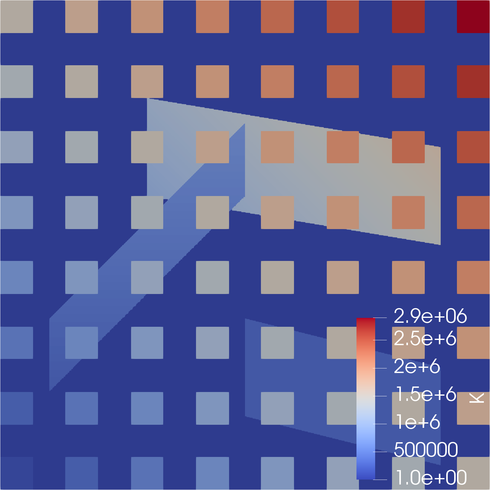
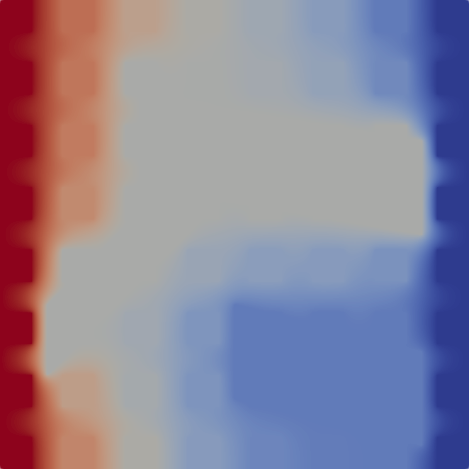
The first test problem considers the scalar elliptic PDE (16) in the unit square or unit cube with the two-dimensional coefficent field given in Figure 2. In the three-dimensional version, the coefficient does not depend on the $z$-coordinate. Boundary conditions are of Dirichlet type on the two planes perpendicular to the $x$-direction and homogeneous Neumann on the rest of the boundary.

Refer to caption
Refer to caption
Figure 2: Permeability and solution for the islands problem in 2d.

5.1.1 Basic two-level experiments

First, we gather some basic experiments that illustrate the behavior of spectral domain decomposition methods. In [16], it was demonstrated that isolated large diffusion coefficients lead to very small eigenvalues that are well separated from the rest. The spectrum of the local GEVP for an interior subdomain contains zero eigenvalues corresponding to the kernel of the bilinear form $a$ (i.e., the constant function here, or the rigid body modes for linear elasticity), then a set of very small eigenvalues related to isolated large coefficients and finally, with some gap, more or less equidistantly spaced eigenvalues. In the spectral DD preconditioner, one has the choice of either including a fixed number $n_{ev}$ of eigenvectors per subdomain into the coarse space or to select all eigenvectors where the corresponding eigenvalue is below a threshold $\eta$. In the first case, the size of the coarse space is controlled, while in the second case the convergence rate is controlled. In most experiments reported below, we will choose the basis for the coarse space according to a threshold $\eta$.

Table 1: Iteration numbers #IT and coarse space sizes $n_{0}$ for a fixed number of subdomains in the two-level method, when varying fine mesh size $h$ and overlap $\delta$ (using Conjugate Gradients, $\mathbb{Q}_{1}$ conforming FEs in 2d, 16 subdomains and a fixed threshold $\eta=0.15$).
Laplace Islands
$\delta\sim h$ $\delta\sim H$ $\delta\sim h$ $\delta\sim H$
$h^{-1}$ #IT $n_{0}$ #IT $n_{0}$ #IT $n_{0}$ #IT $n_{0}$
320 30 56 30 56 31 65 31 65
640 29 114 32 50 27 103 30 59
1280 27 236 25 54 27 240 25 78
2560 26 488 26 54 25 481 24 55

Table 1 investigates how the size of the coarse space in the two-level method depends on the overlap $\delta$. For the standard two-level Schwarz method it is well known that the convergence rate depends on $H/\delta$ [30]. For fixed $H$ (fixed number of subdomains) and decreasing mesh size $h$ the number of iterations does not change when $\delta\sim H$, while it will increase for $\delta\sim h$. For a fixed threshold $\eta$, Table 1 shows that here, the number of iterations $\#IT$ remains constant independent of the choice of the overlap. However, the size of the coarse space $n_{0}$ increases when $\delta\sim h$ while it does not increase when $\delta\sim H$. The table also shows that the size of the coarse space increases only slightly when the homogeneous diffusion coefficient (Laplace) is changed into a heterogeneous diffusion coefficient (Islands).

Table 2: Iteration numbers #IT and coarse space sizes $n_{0}$ for a fixed number of subdomains in the two-level method, when varying polynomial degree $p$ and overlap $\delta$ (using Conjugate Gradients, DG FEs in 2d, $384^{2}$ elements and 256 subdomains).
$\eta=0.15$ $n_{ev}=20$
$\delta=2$ $\delta$ var $\delta=2$ $\delta$ var
$p$ $n_{1}$ #IT $n_{0}$ $\delta$ #IT $n_{0}$ #IT $n_{0}$ $\delta$ #IT $n_{0}$
1 589824 28 1457 2 28 1457 18 5120 2 18 5120
2 1327104 21 3171 3 22 1901 19 5120 3 18 5120
3 2359296 20 5026 3 21 2991 20 5120 3 19 5120
4 3686400 18 8217 4 21 3322 21 5120 4 20 5120
5 5308416 17 13596 4 21 5078 23 5120 4 21 5120
6 7225344 17 17029 5 22 5234 24 5120 5 22 5120

Table 2 investigates the two-level method applied to the DG discretization of the Islands problem. The number of sudomains, as well as the mesh size is fixed in this computation and the polynomial degree $p$ is varied. The number of degrees of freedom $n_{1}$ on the fine level is increasing correspondingly. Experiments with a fixed threshold $\eta=0.15$ or a fixed number of eigenvectors per subdomain $n_{ev}=20$, as well as with fixed and varying overlap $\delta$ are conducted. Using a fixed threshold, the number of iterations is constant or even decreasing while the size of the coarse space $n_{0}$ increases with increasing polynomial degree. With a fixed number of eigenvalues the iteration numbers are slightly increasing at a constant size of the coarse space. In all cases, the preconditioner shows very good performance.

5.1.2 Weak scaling in 2d

Table 3: Conjugate Gradients, $\mathbb{Q}_{1}$ conforming finite elements, $\delta=3h$, $\eta=0.3$.
subdomains 64 256 1024 4096 16384
levels degrees of freedom
finest total 410881 1640961 6558721 26224641 104878081
2 lvl $n_{0}$ 306 1348 5523 22673 91055
3 lvl $n_{0}$ 130 431 1319 3890
4 lvl $n_{0}$ 207 436 891
levels iterations #IT
2 25 26 27 26 26
3 32 31 31 33
4 40 38 38

We now turn to the multilevel method and carry out experiments with a varying number of subdomains. Table 3 conducts a weak scaling experiment for the two-dimensional Islands problem, where the number of degrees of freedom per subdomain is fixed. $\mathbb{Q}_{1}$ conforming finite elements with a fixed overlap $\delta=3h$ and threshold $\eta=0.3$ are used. From left to right the number of subdomains increases from 64 to 16384. The row labelled “finest total” gives the total number of degrees of freedom on the finest level, while the next three rows report $n_{0}$, the size of the level 0 space when 2, 3 or four levels are used. These results show that the size of the coarsest space can be significantly reduced (sizes of intermediate levels are not shown). Finally, the last two rows give iteration numbers when using two, three and four levels. Within each row we observe robustness w.r.t. the number of subdomains. Within each column we observe a moderate increase with the number of levels, but certainly not the exponential increase predicted by Theorem 3.16. The numbers in Table 3 would suggest $\kappa(BA)=O(L^{2})$.

5.1.3 Strong scaling in 3d

Table 4 gives results for the Islands problem in three dimensions using a cell-centered finite volume discretization with two-point flux approximation. Here, the mesh is fixed and the number of subdomains as well as the number of levels are varied. The first set of rows corresponds to the two-level method. We note that the sequential run-time $T_{seq}$ for setting up the preconditioner is reduced by almost a factor 3 when the number of subdomains is increased from 512 to 4096. This is due to the fact that the direct solver and the eigensolver scale nonlinearly with the number of degrees of freedom per subdomain, i.e., smaller is better. But at the same time the size of the coarse problem $n_{0}$ is increasing. The estimated parallel computation time therefore has a minimum at 2048 subdomains with 25.2 seconds. With 4096 subdomains the time for (sequential) factorization of the coarse problem $T_{coarse}$ becomes very large. Also note that there is quite a lot of variability in the times needed to solve the eigenproblems in each subdomain. Minimum and maximum times over all subdomains are reported in the columns labeled $T_{i,min}$ and $T_{i,max}$, respectively. This suggests that more subdomains than available processors should be used in order to average runtimes over several subdomains. The last three rows show corresponding results for a three level method using 4096 subdomains and different numbers of subdomains on the intermediate level. The minimal parallel runtime is achieved for 128 subdomains on level 1, leading to an improvement over the two-level method in that case. Also note that in Table 4 we only report times for constructing the preconditioner. The solution time is only $1/20$ of the setup time.

Table 4: Islands problem in 3d. Fixed problem size $320^{3}$ mesh, 32768000 degrees of freedom. On the finest level $n_{ev}=15$ eigenvectors are taken per subdomain, while for the three level calculation threshold $\eta=0.4$ is used on the intermediate level. Iteration numbers are for the hybrid form of the preconditioner using multiplicative subspace correction over levels and restricted additive Schwarz in each level used within GMRES (restart not reached). Times are in seconds.
$P_{L}$ $P_{L-1}$ #IT $n_{0}$ $T_{seq}$ $T_{par}$ $T_{i,min}$ $T_{i,max}$ $T_{coarse}$
two level method
512 1 12 7680 63613 191.3 70.3 176.2 0.47
1024 1 12 15360 35817 58.4 18.2 49.8 1.3
2048 1 14 30720 18781 25.2 4.9 13.2 5.1
4096 1 13 61441 19982 33.5 2.2 7.0 20.1
three level method
4096 32 15 1387 21168 55.9 9.8 42.3 0.27
4096 64 15 1817 20725 27.7 2.5 15.1 0.18
4096 128 16 2569 20549 18.4 0.59 6.2 0.15

5.2 SPE10 Problem

Refer to caption
Figure 3: Permeability field for the SPE10 problem.
Table 5: SPE10 problem. Discretization schemes: $\mathbb{Q}_{1}$ conforming finite elements (CG), cell-centered finite volumes (FV) and DG-$\mathbb{Q}_{1}$ are compared for two and three levels. Times are in seconds.
CG, $n_{L}=9124731$ CCFV, $n_{L}=8976000$ DG, $n_{L}=8976000$
$P_{L},P_{L-1}$ #IT $n_{0}$ $T_{par}$ #IT $n_{0}$ $T_{par}$ #IT $n_{0}$ $T_{par}$
two levels, $\eta=0.3$
256 24 7237 133.8 25 7502 49.2 22 8366 233.5
512 24 9830 60.4 23 10600 21.6 21 13690 124.9
1024 28 21881 22.3 25 25753 12.3 24 31637 42.4
2048 25 29023 15.7 25 35411 11.2 25 46844 36.7
three levels, $\eta=0.3$
256, 16 29 1222 151.4 29 1364 70.3 31 1683 273.2
512, 16 27 1228 77.8 28 1446 47.4 28 1762 186.8
1024, 32 36 3145 46.3 34 3487 47.3 33 5476 231.4
2048, 32 31 3120 40.1 35 3421 49.9 36 5359 204.8

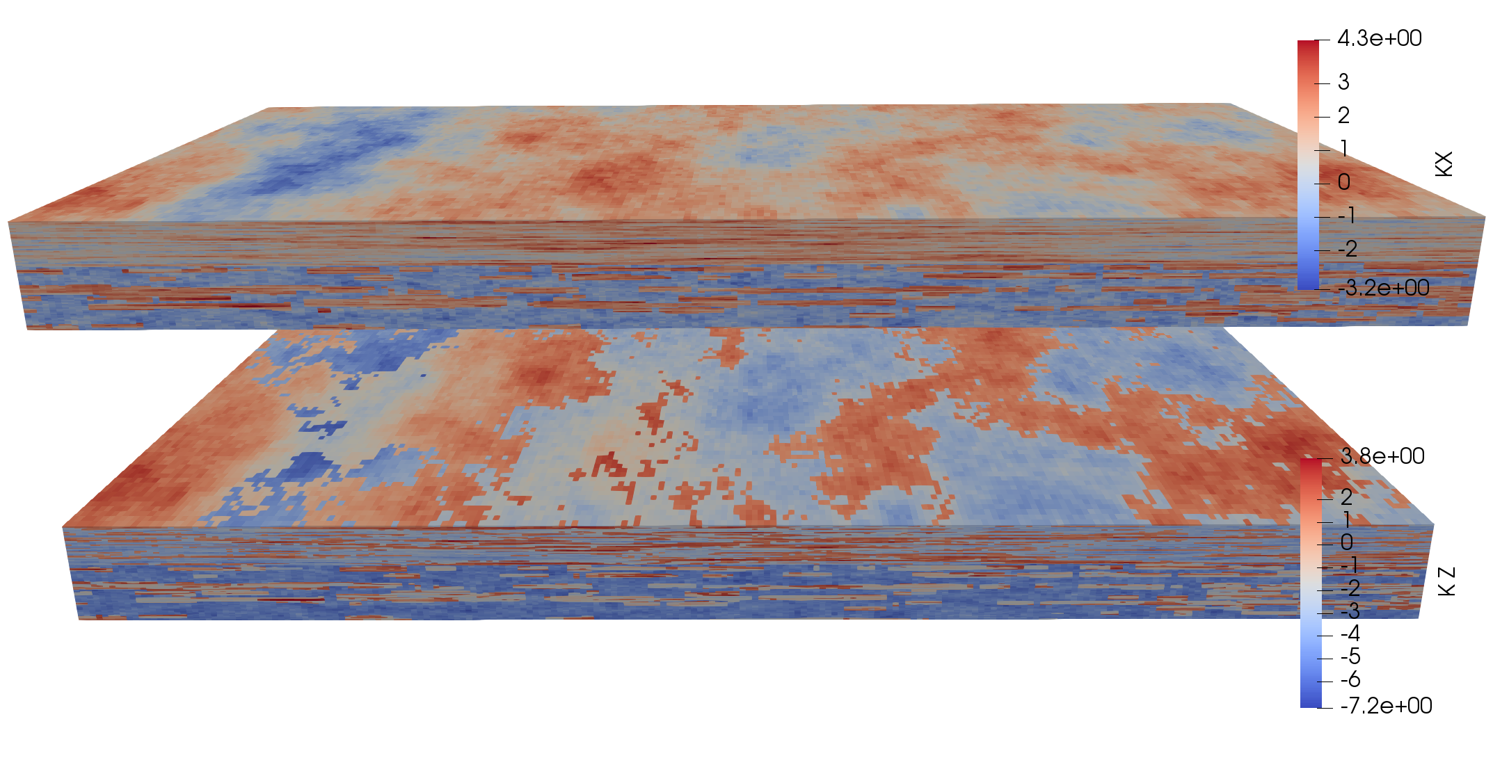
Next, we consider the SPE10 problem [9]. Originally intended as a benchmark for multiscale methods it is often used as a test problem for preconditioners as well. The scalar elliptic problem (16) is solved in a box-shaped domain, discretized with an axiparallel and equidistant hexahedral mesh consisting of 1122000 elements. The diffusion tensor $K(x)$ is diagonal and highly variably. The $x$ and $y$ components are identical and vary over 7 orders of magnitude. The $z$ component varies over 11 orders of magnitude. Figure 3 shows the permeability.

Table 5 reports results for the SPE10 problem where we concentrate on the comparison of the performance for different discretization schemes: conforming $\mathbb{Q}_{1}$ finite elements on a refined mesh, cell-centered finite volumes on a refined mesh and DG-$\mathbb{Q}_{1}$ on the original mesh. All problems have roughly the same number of degrees of freedom, i.e., around 9 million. Results for two and three levels using up to 2048 subdomains are given. The hybrid form of the preconditioner using multiplicative subspace correction over levels and restricted additive Schwarz in each level is used within GMRES (restart not reached) For each configuration we report number of iterations, size of the coarsest space and estimated parallel runtime for setting up the preconditioner. We observe: the number of iterations is independent of the number of subdomains and the discretization scheme used. From two to three levels a moderate increase in the number of iterations is observed. However, the problem size is too small to achieve an improvement in runtime through the use of more than two levels.

5.3 Composites Problem

We report results on modelling carbon fibre composite materials from aerospace engineering, described in detail in [26, 7]. The setup is similar to the one in [26, p. 271], except that the domain is flattened out and consists of only 9 ply layers and 8 interface (resin) layers. The equations of linear elasticity are solved in three dimensions using $\mathbb{Q}_{2}$ serendipity elements resulting in 10523067 degrees of freedom. Table 6 shows results for 1024 subdomains using 2, 3 or 4 levels using the preconditioner in its hybrid form within GMRES (multiplicative over levels, restricted additive Schwarz within levels, restart not reached). While the two-level method converges in 13 steps, the three and four level methods need 31 and 35 iterations, respectively. The maximum number of degrees of freedom in any coarse subdomain is significantly reduced in the three and four level methods compared to the two level method.

Table 6: Carbon fibre composite problem. 9 ply layers (thickness 0.23mm), 8 resin layers (thickness 0.02mm), discretized with $256\times 64\times 52$ mesh using $\mathbb{Q}_{2}$ serendipity elements. Threshold $\eta=0.35$.
subdomains max dofs/subdomain #IT
level 3 2 1 0 3 2 1 0
1024 1 28791 21565 13
1024 32 1 28791 1260 914 31
1024 128 16 1 28791 546 515 273 35

6 Conclusions

In this paper we extended the GenEO coarse space introduced in [29] from two to multiple levels and used it in the construction of multilevel preconditioners which are robust in the fine mesh size, number of subdomains and coefficient variations. The number of levels in the hierarchy is typically moderate since aggressive coarsening is used. While the theory predicts an exponential increase of the condition number of the preconditioned system with the number of levels numerical results suggest that the increase is moderate. We believe that novel approximation theory for related spectral coarse spaces in [22] will allow us to improve these theoretical results in future work. In addition, the theory presented is more general than [29], extending also to different discretization schemes as well as to different variants of the generalized eigenproblem. In particular, we were able to analyse the preconditioner for discontinuous Galerkin discretizations of scalar elliptic problems. Numerical results illustrate the robustness of the preconditioner for heterogeneous diffusion as well as linear elasticity problems. Improvements over the two-level method could be demonstrated for a three-dimensional problem with 30 million degrees of freedom.

Acknowledgments

This work is supported by the Deutsche Forschungsgemeinschaft (DFG, German Research Foundation) under Germany’s Excellence Strategy EXC 2181/1 - 390900948 (the Heidelberg STRUCTURES Excellence Cluster). P. B. would like to thank Hussam Al Daas for discussions.

References

  • [1] J. E. Aarnes, Efficient domain decomposition methods for elliptic problems arising from flows in heterogeneous porous media, Computing and Visualization in Science, 8 (2005), pp. 93–106, https://doi.org/10.1007/s00791-005-0155-6.
  • [2] H. Al Daas and L. Grigori, A class of efficient locally constructed preconditioners based on coarse spaces, SIAM Journal on Matrix Analysis and Applications, 40 (2019), pp. 66–91, https://doi.org/10.1137/18M1194365.
  • [3] H. Al Daas, L. Grigori, P. Jolivet, and P.-H. Tournier, A multilevel Schwarz preconditioner based on a hierarchy of robust coarse spaces. Preprint hal-02151184v2f, Dec. 2020, https://hal.archives-ouvertes.fr/hal-02151184.
  • [4] R. E. Alcouffe, A. Brandt, J. E. Dendy, Jr., and J. W. Painter, The multi-grid method for the diffusion equation with strongly discontinuous coefficients, SIAM Journal on Scientific and Statistical Computing, 2 (1981), pp. 430–454, https://doi.org/10.1137/0902035.
  • [5] P. Bastian, M. Blatt, A. Dedner, N.-A. Dreier, C. Engwer, R. Fritze, C. Gräser, C. Grüninger, D. Kempf, R. Klöfkorn, M. Ohlberger, and O. Sander, The Dune framework: Basic concepts and recent developments, Computers & Mathematics with Applications, 81 (2021), pp. 75–112, https://doi.org/10.1016/j.camwa.2020.06.007.
  • [6] P. Bastian, M. Blatt, A. Dedner, C. Engwer, R. Klöfkorn, R. Kornhuber, M. Ohlberger, and O. Sander, A generic grid interface for parallel and adaptive scientific computing. Part II: Implementation and tests in DUNE, Computing, 82 (2008), pp. 121–138, https://doi.org/10.1007/s00607-008-0004-9.
  • [7] R. Butler, T. Dodwell, A. Reinarz, A. Sandhu, R. Scheichl, and L. Seelinger, High-performance dune modules for solving large-scale, strongly anisotropic elliptic problems with applications to aerospace composites, Computer Physics Communications, 249 (2020), p. 106997, https://doi.org/10.1016/j.cpc.2019.106997.
  • [8] Y. Chen, T. A. Davis, W. W. Hager, and S. Rajamanickam, Algorithm 887: Cholmod, supernodal sparse Cholesky factorization and update/downdate, ACM Trans. Math. Softw., 35 (2008), https://doi.org/10.1145/1391989.1391995.
  • [9] M. Christie, M. Blunt, et al., Tenth SPE comparative solution project: A comparison of upscaling techniques, in SPE Reservoir Simulation Symposium, Society of Petroleum Engineers, 2001, https://doi.org/10.2118/72469-PA.
  • [10] T. A. Davis, Algorithm 832: Umfpack v4.3—an unsymmetric-pattern multifrontal method, ACM Trans. Math. Softw., 30 (2004), p. 196–199, https://doi.org/10.1145/992200.992206.
  • [11] V. Dolean, P. Jolivet, and F. Nataf, An Introduction to Domain Decomposition Methods, Society for Industrial and Applied Mathematics, Philadelphia, PA, 2015, https://doi.org/10.1137/1.9781611974065.
  • [12] V. Dolean, F. Nataf, R. Scheichl, and N. Spillane, Analysis of a two-level Schwarz method with coarse spaces based on local Dirichlet-to-Neumann maps, Computational Methods in Applied Mathematics, 12 (2012), pp. 391 – 414, https://doi.org/10.2478/cmam-2012-0027.
  • [13] Y. Efendiev, J. Galvis, R. Lazarov, and J. Willems, Robust domain decomposition preconditioners for abstract symmetric positive definite bilinear forms, ESAIM: M2AN, 46 (2012), pp. 1175–1199, https://doi.org/10.1051/m2an/2011073.
  • [14] A. Ern and J. Guermond, Theory and Practice of Finite Element Methods, Springer, 2004.
  • [15] A. Ern, A. F. Stephansen, and P. Zunino, A discontinuous Galerkin method with weighted averages for advection–diffusion equations with locally small and anisotropic diffusivity, IMA Journal of Numerical Analysis, 29 (2008), pp. 235–256, https://doi.org/10.1093/imanum/drm050.
  • [16] J. Galvis and Y. Efendiev, Domain decomposition preconditioners for multiscale flows in high-contrast media, Multiscale Modeling & Simulation, 8 (2010), pp. 1461–1483, https://doi.org/10.1137/090751190.
  • [17] I. G. Graham, P. O. Lechner, and R. Scheichl, Domain decomposition for multiscale PDEs, Numerische Mathematik, 106 (2007), pp. 589–626, https://doi.org/10.1007/s00211-007-0074-1.
  • [18] R. Haferssas, P. Jolivet, and F. Nataf, A robust coarse space for optimized Schwarz methods: SORAS-GenEO-2, Comptes Rendus Mathematique, 353 (2015), pp. 959–963, https://doi.org/10.1016/j.crma.2015.07.014.
  • [19] G. Karypis and V. Kumar, Multilevel $k$-way partitioning scheme for irregular graphs, Journal of Parallel and Distributed Computing, 48 (1998), pp. 96 – 129, https://doi.org/10.1006/jpdc.1997.1404.
  • [20] R. B. Lehoucq, D. C. Sorensen, and C. Yang, ARPACK Users’ Guide, Society for Industrial and Applied Mathematics, 1998, https://epubs.siam.org/doi/abs/10.1137/1.9780898719628.
  • [21] J.-Y. L’Excellent, Multifrontal Methods: Parallelism, Memory Usage and Numerical Aspects, habilitation à diriger des recherches, Ecole normale supérieure de lyon - ENS LYON, Sept. 2012, https://tel.archives-ouvertes.fr/tel-00737751.
  • [22] C. Ma, R. Scheichl, and T. Dodwell, Novel design and analysis of generalized FE methods based on locally optimal spectral approximations. Preprint arXiv:2103.09545, Mar. 2021, https://arxiv.org/abs/2103.09545.
  • [23] A. Napov and Y. Notay, An algebraic multigrid method with guaranteed convergence rate, SIAM Journal on Scientific Computing, 34 (2012), pp. A1079–A1109, https://doi.org/10.1137/100818509.
  • [24] F. Nataf, H. Xiang, and V. Dolean, A two level domain decomposition preconditioner based on local Dirichlet-to-Neumann maps, Comptes Rendus Mathematique, 348 (2010), pp. 1163 – 1167, https://doi.org/10.1016/j.crma.2010.10.007.
  • [25] C. Pechstein and R. Scheichl, Weighted Poincaré inequalities, IMA Journal of Numerical Analysis, 33 (2013), pp. 652–686, https://doi.org/10.1093/imanum/drs017.
  • [26] A. Reinarz, T. Dodwell, T. Fletcher, L. Seelinger, R. Butler, and R. Scheichl, Dune-composites – a new framework for high-performance finite element modelling of laminates, Composite Structures, 184 (2018), pp. 269 – 278, https://doi.org/10.1016/j.compstruct.2017.09.104.
  • [27] R. Scheichl, P. S. Vassilevski, and L. T. Zikatanov, Mutilevel methods for elliptic problems with highly varying coefficients on non-aligned coarse grids, SIAM Journal on Numerical Analysis, 50 (2012), pp. 1675–1694, https://epubs.siam.org/doi/abs/10.1137/100805248.
  • [28] B. Smith, P. Bjørstad, and W. Gropp, Domain Decomposition – Parallel Multilevel Methods for Elliptic Partial Differential Equations, Cambridge University Press, 1996.
  • [29] N. Spillane, V. Dolean, P. Hauret, F. Nataf, C. Pechstein, and R. Scheichl, Abstract robust coarse spaces for systems of PDEs via generalized eigenproblems in the overlaps, Numerische Mathematik, 126 (2014), pp. 741–770, https://doi.org/10.1007/s00211-013-0576-y.
  • [30] A. Toselli and O. Widlund, Domain Decomposition Methods – Algorithms and Theory, Springer, Berlin Heidelberg, 2005.
  • [31] J. Willems, Robust multilevel methods for general symmetric positive definite operators, SIAM Journal on Numerical Analysis, 52 (2014), pp. 103–124, https://doi.org/10.1137/120865872.
  • [32] J. Xu, Iterative methods by space decomposition and subspace correction, SIAM Review, 34 (1992), pp. 581–613, https://doi.org/10.1137/1034116.
  • [33] J. Xu and L. Zikatanov, Algebraic multigrid methods, Acta Numerica, 26 (2017), p. 591–721, https://doi.org/10.1017/S0962492917000083.