Global Neighbor Sampling for Mixed CPU-GPU Training on Giant Graphs

Abstract.

Graph neural networks (GNNs) are powerful tools for learning from graph data and are widely used in various applications such as social network recommendation, fraud detection, and graph search. The graphs in these applications are typically large, usually containing hundreds of millions of nodes. Training GNN models on such large graphs efficiently remains a big challenge. Despite a number of sampling-based methods have been proposed to enable mini-batch training on large graphs, these methods have not been proved to work on truly industry-scale graphs, which require GPUs or mixed-CPU-GPU training. The state-of-the-art sampling-based methods are usually not optimized for these real-world hardware setups, in which data movement between CPUs and GPUs is a bottleneck. To address this issue, we propose Global Neighborhood Sampling that aims at training GNNs on giant graphs specifically for mixed-CPU-GPU training. The algorithm samples a global cache of nodes periodically for all mini-batches and stores them in GPUs. This global cache allows in-GPU importance sampling of mini-batches, which drastically reduces the number of nodes in a mini-batch, especially in the input layer, to reduce data copy between CPU and GPU and mini-batch computation without compromising the training convergence rate or model accuracy. We provide a highly efficient implementation of this method and show that our implementation outperforms an efficient node-wise neighbor sampling baseline by a factor of $2\times-4\times$ on giant graphs. It outperforms an efficient implementation of LADIES with small layers by a factor of $2\times-14\times$ while achieving much higher accuracy than LADIES. We also theoretically analyze the proposed algorithm and show that with cached node data of a proper size, it enjoys a comparable convergence rate as the underlying node-wise sampling method.

1. Introduction

Many real world data come naturally in the form of graphs; e.g., social networks, recommendation, gene expression networks, and knowledge graphs. In recent years, Graph Neural Networks (GNNs) (Kipf and Welling, [n. d.]; Velickovic et al., [n. d.]; Hamilton et al., 2017) have been proposed to learn from such graph-structured data and have achieved outstanding performance. Yet, in many applications, graphs are usually large, containing hundreds of millions to billions of nodes and tens to hundreds of billions of edges. Learning on such giant graphs is challenging due to the limited amount of memory available on a single GPU or a single machine. As such, mini-batch training is used to train GNN models on such giant graphs. However, due to the connectivities between nodes, computing the embeddings of a node with multi-layer GNNs usually involves in many nodes in a mini-batch. This leads to substantial computation and data movement between CPUs and GPUs in mini-batch training and makes training inefficient.

To remedy this issue, various GNN training methods have been developed to reduce the number of nodes in a mini-batch (Hamilton et al., 2017; Zeng et al., 2019; Chen et al., 2018; Zou et al., 2019; Liu et al., 2020). Node-wise neighbor sampling used by GraphSage (Hamilton et al., 2017) samples a fixed number of neighbors for each node independently. Even though it reduces the number of neighbors sampled for a mini-batch, the number of nodes in each layer still grows exponentially. FastGCN (Chen et al., 2018) and LADIES (Zou et al., 2019) sample a fixed number of nodes in each layer, which results in isolated nodes when used on large graphs. In addition, LADIES requires significantly more computation to sample neighbors and can potentially slow down the overall training speed. The work by Liu et al. (Liu et al., 2020) tries to alleviate the neighborhood explosion and reduce the sampling variance by applying a bandit sampler. However, this method leads to very large sampling overhead and does not scale to large graphs. These sampling methods are usually evaluated on small to medium-size graphs. When applying them to industry-scale graphs, they have suboptimal performance or substantial computation overhead as we discovered in our experiments.

To address some of these problems and reduce training time, LazyGCN  (Ramezani et al., 2020) periodically samples a mega-batch of nodes and reuses it to sample further mini-batches. By loading each mega-batch in GPU memory once, LazyGCN can mitigate data movement/preparation overheads. However, in order to match the accuracy of standard GNN training LazyGCN requires very large mega-batches (cf. Figure 4), which makes it impractical for graphs with hundreds of millions of nodes.

We design an efficient and scalable sampling method that takes into account the characteristics of training hardware into consideration. GPUs are the most efficient hardware for training GNN models. Due to the small GPU memory size, state-of-the-art GNN frameworks, such as DGL (Wang et al., 2019) and Pytorch-Geometric (Fey and Lenssen, 2019), keep the graph data in CPU memory and perform mini-batch computations on GPUs when training GNN models on large graphs. We refer to this training strategy as mixed CPU-GPU training. The main bottleneck of mixed CPU-GPU training is data copy between CPUs and GPUs (cf. Figure 1). Because mini-batch sampling occurs in CPU, we need a low-overhead sampling algorithm to enable efficient training. Motivated by the hardware characteristics, we developed the Global Neighborhood Sampling (GNS) approach that samples a global set of nodes periodically for all mini-batches. The sampled set is small so that we can store all of their node features in GPU memory and we refer this set of nodes as cache. The cache is used for neighbor sampling in a mini-batch. Instead of sampling any neighbors of a node, GNS gives the priorities of sampling neighbors that exist in the cache. This is a fast way of biasing node-wise neighbor sampling to reduce the number of distinct nodes of each mini-batch and increase the overlap between mini-batches. When coupled with GPU cache, this method drastically reduces the amount of data copy between GPU and CPU to speed up training. In addition, we deploy importance sampling that reduces the sampling variance and also allows us to use a small cache size to train models.

We develop a highly optimized implementation of GNS and compare it with efficient implementations of other sampling methods provided by DGL, including node-wise neighbor sampling and LADIES. We show that GNS achieves state-of-the-art model accuracy while speeding up training by a factor of $2\times-4\times$ compared with node-wise sampling and by a factor of $2\times-14\times$ compared with LADIES.

The main contributions of the work are described below:

1. We analyze the existing sampling methods and demonstrate their main drawbacks on large graphs.

2. We develop an efficient and scalable sampling algorithm that addresses the main overhead in mixed CPU-GPU mini-batch training and show a substantial training speedup compared with efficient implementations of other training methods.

3. We demonstrate that this sampling algorithm can train GNN models on graphs with over 111 millions of nodes and 1.6 billions of edges.

2. Background

In this section, we review GNNs and several state-of-the-art sampling-based training algorithms, including node-wise neighbor sampling methods and layer-wise importance sampling methods. The fundamental concepts of mixed-CPU-GPU training architecture is introduced. We discuss the limitations of state-of-the-art sampling methods in mixed-CPU-GPU training.

2.1. Existing GNN Training Algorithms

Full-batch GNN Given a graph $\mathcal{G(\mathcal{V},\mathcal{E})}$, the input feature of node $v\in\mathcal{V}$ is denoted as $\mathbf{h}_{v}^{(0)}$, and the feature of the edge between node $v$ and $u$ is represented as $\mathbf{w}_{uv}$. The representation of node $v\in\mathcal{V}$ at layer $\ell$ can be derived from a GNN model given by:

(1) $$\mathbf{h}_{v}^{\ell}=g(\mathbf{h}_{v}^{\ell-1},\bigcup_{u\in\mathcal{N}(v)}f(\mathbf{h}_{u}^{\ell-1},\mathbf{h}_{v}^{\ell-1},\mathbf{w}_{uv})),$$

where $f$, $\bigcup$ and $g$ are pre-defined or parameterized functions for computing feature data, aggregating data information, and updating node representations, respectively. For instance, in GraphSage training (Hamilton et al., 2017), the candidate aggregator functions include mean aggregator (Kipf and Welling, [n. d.]), LSTM aggregator (Hochreiter and Schmidhuber, 1997), and max pooling aggregator (Qi et al., 2017). The function $g$ is set as nonlinear activation function.

Given training dataset $\{(\mathbf{x}_{i},y_{i})\}_{v_{i}\in\mathcal{V}_{s}}$, the parameterized functions will be learned by minimizing the loss function:

(2) $$\mathcal{L}=\frac{1}{|\mathcal{V}_{s}|}\sum_{v_{i}\in\mathcal{V}_{s}}\ell(y_{i},\mathbf{z}_{i}^{L}),$$

where $\ell(\cdot,\cdot)$ is a loss function, $\mathbf{z}_{i}^{L}$ is the output of GNN with respect to the node $v_{i}\in\mathcal{V}_{s}$ where $\mathcal{V}_{S}$ represents the set of training nodes. For full-batch optimization, the loss function is optimized by gradient descent algorithm where the gradient with respect to each node $v_{i}\in\mathcal{V}_{S}$ is computed as $\frac{1}{|\mathcal{V}_{s}|}\sum_{v_{i}\in\mathcal{V}_{S}}\nabla\ell(y_{i},\mathbf{z}_{i}^{(L)})$. During the training process, full-batch GNN requires to store and aggregate representations of all nodes across all layers. The expensive computation time and memory costs prohibit full-batch GNN from handling large graphs. Additionally, the convergence rate of full-batch GNN is slow because model parameters are updated only once at each epoch.

Mini-batch GNN To address this issue, a mini-batch training scheme has been developed which optimizes via mini-batch stochastic gradient descent $\frac{1}{|\mathcal{V}_{B}|}\sum_{v_{i}\in\mathcal{V}_{B}}\nabla\ell(y_{i},\mathbf{z}_{i}^{L})$ where $\mathcal{V}_{B}\in\mathcal{V}_{S}$. These methods first uniformly sample a set of nodes from the training set, known as target nodes, and sample neighbors of these target nodes to form a mini-batch. The focus of the mini-batch training methods is to reduce the number of neighbor nodes for aggregation via various sampling strategies to reduce the memory and computational cost. The state-of-the-art sampling algorithm is discussed in the sequel.

Node-wise Neighbor Sampling Algorithms. Hamilton et al. (Hamilton et al., 2017) proposed an unbiased sampling method to reduce the number of neighbors for aggregation via neighbor sampling. It randomly selects at most $s_{\text{node}}$ (defined as fan-out parameter) neighborhood nodes for every target node; followed by computing the representations of target nodes via aggregating feature data from the sampled neighborhood nodes. Based on the notations in (1), the representation of node $v\in\mathcal{V}$ at layer $\ell$ can be described as follows:

(3) $$\mathbf{h}_{v}^{\ell}=g\bigg{(}\mathbf{h}_{v}^{\ell-1},\bigcup_{u\in\mathcal{N}_{\ell}(v)}f\big{(}\frac{1}{s_{\text{node}}}\mathbf{h}_{u}^{\ell-1},\mathbf{h}_{v}^{\ell-1}\big{)}\bigg{)},$$

where $\mathcal{N}_{\ell}(v)$ is the sampled neighborhood nodes set at $\ell$-th layer such that $|\mathcal{N}_{\ell}(v)|=s_{\text{node}}$. The neighbor sampling procedure is repeated recursively on target nodes and their sampled neighbors when dealing with multiple-layer GNN. Even though node-wise neighbor sampling scheme addresses the memory issue of GNN, there exists excessive computation under this scheme because the scheme still results in exponential growth of neighbor nodes with the number of layers. This yields a large volume of data movement between CPU and GPU for mixed CPU-GPU training.

Layer-wise Importance Sampling Algorithms. To address the scalability issue, Chen et al. (Chen et al., 2018) proposed an advanced layer-wise method called FastGCN. Compared with node-wise sampling method, it yields extra variance when sampling a fixed number of nodes for each layer. To address the variance issue, it performs degree-based importance sampling on each layer. The representation of node $v\in\mathcal{V}$ at layer $\ell$ of FastGCN model is described as follows:

(4) $$\mathbf{h}_{v}^{\ell}=g\bigg{(}\mathbf{h}_{v}^{\ell-1},\bigcup_{u\in q(v)}f\big{(}\frac{1}{s_{\text{layer}}}\mathbf{h}_{u}^{\ell-1}/{q_{u}},\mathbf{h}_{v}^{\ell-1}\big{)}\bigg{)},$$

where the sample size denotes as $s_{\text{layer}}$, $q(v)$ is the distribution over $v\in\mathcal{V}$ and $q_{u}$ is the probability assigned to node $u$. A major limitation is that FastGCN performs sampling on every layer independently, which yields approximate embeddings with large variance. Moreover, the subgraph sampled by FastGCN is not representative to the original graph. This leads to poor performance and the number of sampled nodes required to guarantee convergence during training process is large.

The work by Zhou et al. (Zou et al., 2019) proposed a sampling algorithm known as LAyer-Dependent ImportancE Sampling (LADIES) to address the limitation of FastGCN and exploit the connection between different layers. Specifically, at $\ell$-th layer, LADIES samples nodes reachable from the nodes in the previous layer. However, this method (Zou et al., 2019) comes with cost. To ensure the node connectivity between layers, the method needs to extract and merge the entire neighborhood of all nodes in the previous layer and compute the sampling probability for all candidate nodes in the next layer. Thus, this sampling method has significantly higher computation overhead. Furthermore, when applying this method on a large graph, it still constructs a mini-batch with many isolated nodes, especially for nodes in the first layer (Table 5).

LazyGCN. Even though layer-wise sampling methods effectively address the neighborhood explosion issue, they failed to investigate computational overheads in preprocessing data and loading fresh samples during training. Ramezan et al. (Ramezani et al., 2020) proposed a framework called LazyGCN which decouples the frequency of sampling from the sampling strategy. It periodically samples mega-batches and effectively reuses mega-batches to generate mini-batches and alleviate the preprocessing overhead. There are some limitations in the LazyGCN setting. First, this method requires large mini-batches to guarantee model accuracy. For example, their experiments on Yelp and Amazon dataset use the batch size of 65,536. This batch size is close to the entire training set, yielding overwhelming overhead in a single mini-batch computation. Its performance deteriorates for smaller batch sizes even with sufficient epochs (Figure 4). Second, their evaluation is based on inefficient implementations with very large sampling overhead. In practice, the sampling computation overhead is relatively low in the entire mini-batch computation (Figure 1) when using proper development tools.

Even though both GNS and LazyGCN cache data in GPU to accelerate computation in mixed CPU-GPU training, they use very different strategies for caching. LazyGCN caches the entire graph structure of multiple mini-batches sampled by node-wise neighbor sampling or layer-wise sampling and suffers from the problems in these two algorithms. Due to the exponential growth of the neighborhood size in node-wise neighbor sampling, LazyGCN cannot store a very large mega-batch in GPU and can generate few mini-batches from the mega-batch. Our experiments show that LazyGCN runs out of GPU memory even with a small mega-batch size and mini-batch size on large graphs (OAG-paper and OGBN-papers100M in Table 2). Layer-wise sampling may result in many isolated nodes in a mini-batch. In addition, LazyGCN uses the same sampled graph structure when generating mini-batches from mega-batches, this potentially leads to overfit. In contrast, GNS cache nodes and use the cache to reduce the number of nodes in a mini-batch; GNS always sample a different graph structure for each mini-batch and thus it is less likely to overfit.

2.2. Mixed CPU-GPU training

Due to limited GPU memory, state-of-the art GNN framework (e.g., DGL (Wang et al., 2019) and Pytorch Geometric (Fey and Lenssen, 2019)) train GNN models on large graph data by storing the whole graph data in CPU memory and performing mini-batch computation on GPUs. This allows users to take advantage of large CPU memory and use GPUs to accelerate GNN training. In addition, mixed CPU-GPU training makes it easy to scale GNN training to multiple GPUs or multiple machines (Zheng et al., 2020).

Mixed CPU-GPU training strategy usually involves six steps: 1) sample a mini-batch from the full graph, 2) slice the node and edge data involved in the mini-batch from the full graph, 3) copy the above sliced data to GPU, 4) perform forward computation on the mini-batch, 5) perform backward propagation, and 6) run the optimizer and update model parameters. Steps 1–2 are done by the CPU, whereas steps 4–6 are done by the GPU.

We benchmark the mini-batch training of GraphSage (Hamilton et al., 2017) models with node-wise neighbor sampling provided by DGL, which provides very efficient neighbor sampling implementation and graph kernel computation for GraphSage. Figure 1 shows the breakdown of the time required to train GraphSage on the OGBN-products graph and the OAG-paper graph (see Table 2 for dataset information). Even though sampling happens in CPU, its computation accounts for 10% or less with sufficient optimization and parallelization. However, the speed of copying node data in CPU (step 2) is limited by the CPU memory bandwidth and moving data to GPU (step 3) is limited by the PCIe bandwidth. Data copying accounts for most of the time required by mini-batch training. For example, the training spends  60% and  80% of the per mini-batch time in copying data from CPU to GPU on OGBN-products and OAG-paper, respectively. The training on OAG-paper takes significantly more time on data copy because OAG-paper has 768-dimensional BERT embeddings (Devlin et al., 2019) as node features, whereas OGBN-products uses 100-dimensional node features.

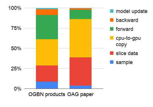
Figure 1. Runtime breakdown (%) of each component in mini-batch training for an efficient GraphSage implementation in DGL.

These results show that when the different components of mini-batch training are highly-optimized, the main bottleneck of mixed CPU-GPU training is data copy (both data copy in CPU and between CPU and GPUs). To speed up training, it is essential to reduce the overhead of data copy, without significantly increasing the overhead of other steps.

3. Global Neighbor Sampling (GNS)

To overcome the drawbacks of the existing sampling algorithms and tackle the unique problems in mixed CPU-GPU training, we developed a new sampling approach, called Global Neighborhood Sampling (GNS), that has low computational overhead and reduces the number of nodes in a mini-batch without compromising the model accuracy and convergence rate. Like node-wise and layer-wise sampling, GNS uses mini-batch training to approximate the full-batch GNN training on giant graphs.

Table 1. Summary of Notations and Definitions

$\mathcal{G}=(\mathcal{V},\mathcal{E})$	$\mathcal{G}$ denotes the graph consist of set of $|\mathcal{V}|$ nodes and $|\mathcal{E}$ | edges.
$L,K$	$L$ is the total number of layers in GCN, and $K$ is the dimension of embedding vectors (for simplicity, assume it is the same across all layers).
$b,s_{node},s_{layer}$	For batch-wise sampling, $b$ denotes the batch size, $s_{node}$ is the number of sampled neighbors per node for node-wise sampling, and $s_{layer}$ is number of sampled nodes per layer for layer-wise sampling.
$\mathcal{N}(v)$	Denotes the set of neighbors of node $v\in\mathcal{V}$.
$\mathcal{N}_{\ell}(v)$	Denotes the set of sampled neighbors of node $v\in\mathcal{V}$ at $\ell$-th layer.
$\mathcal{N}_{\ell}^{\text{u}}(v)$	Denotes the set of neighbors of node $v\in\mathcal{V}$ at $\ell$-th layer sampled uniformly at random.
$\mathcal{N}_{C}(v)$	Denotes the set of neighbors of node $v\in\mathcal{V}$ in the cache.
$\mathcal{C},p^{\text{cache}}_{v}$	Denotes the set of cached nodes which are sampled from $\mathcal{V}$ corresponding to the probability of $p^{\text{cache}}_{v}$ for $v\in\mathcal{V}$.
$p^{(\ell)}_{v}$	Denotes importance sampling coefficients with respect to the node $v\in\mathcal{V}$ at $\ell$-th layer in Algorithm 1.
$\mathcal{V}_{S}$, $|\mathcal{V}_{S}|$	Denotes the training set and the size of the training set.
target node	The node in the mini-batch where the mini-batch is sampled at random from the training node set.
$\mathcal{V}_{B}$, $|\mathcal{V}_{B}|$	Denotes the set of target nodes and the number of target nodes in a mini-batch.

3.1. Overview of GNS

Instead of sampling neighbors independently like node-wise neighbor sampling, GNS periodically samples a global set of nodes following a probability distribution $\mathcal{P}$ to assist in neighbor sampling. $\mathcal{P}_{i}$ defines the probability of node $i$ in the graph being sampled and placed in the set. Because GNS only samples a small number of nodes to form the set, we can copy all of the node features in the set to GPUs. Thus, we refer to the set of nodes as node cache $\mathcal{C}$. When sampling neighbors of a node, GNS prioritizes the sampled neighbors from the cache and samples additional neighbors outside the cache only if the cache does not provide sufficient neighbors.

Because the nodes in the cache are sampled, we can compute the node sampling probability from the probability of a node appearing in the cache, i.e., $\mathcal{P}$. We rescale neighbor embeddings by importance sampling coefficients $p_{u}^{(\ell)}$ from $\mathcal{P}$ in the mini-batch forward propagation so that the expectation of the aggregation of sampled neighbors is the same as the aggregation of the full neighborhood.

(5) $$\mathbb{E}\left(\sum_{u\in\mathcal{N}_{\ell}(v)}p_{u}^{(\ell)}*h_{u}^{\ell}\right)=\sum_{u\in\mathcal{N}(v)}h_{u}^{\ell}$$

Algorithm 1 illustrates the entire training process.

In the remaining sections, we first discuss the cache sampling in Section 3.2. We explain the sampling procedure in Section 3.3. To reduce the variance in GNS, an importance sampling scheme is further developed in Section 3.4. We then establish the convergence rate of GNS which is inspired by the paper (Ramezani et al., 2020). It shows that under mild assumption, GNS enjoys comparable convergence rate as underlying node-wise sampling in training, which is demonstrated in Section 3.5. The notations and definition used in the following is summarized in Table 1.

Input : Graph $\mathcal{G(\mathcal{V},\mathcal{E})}$;

list of target nodes of minibatches $\{\mathcal{B}_{1},\cdots,\mathcal{B}_{M}\}$;

input features $\{\mathbf{x}_{v},\forall v\in\mathcal{V}\}$;

number of epochs $T$;

depth $L$; weight matrices $\mathbf{W}^{\ell},\forall\ell\in\{1,...,L\}$;

cache sampling probability $\mathcal{P}$;

nonlinear activation function $g$;

differentiable aggregator functions $f_{\ell},\forall\ell\in\{1,...,L\}$.

1

Output : Vector representations $\mathbf{z}_{v}$ for all $v\in\mathcal{B}$

1:  for $t=0$ to $T$ do

2:     $\mathcal{C}\leftarrow sample\_cache(\mathcal{V},\mathcal{P},\{\mathcal{B}_{1},\cdots,\mathcal{B}_{M}\})$

3:     for $\mathcal{B}\in\{\mathcal{B}_{1},\cdots,\mathcal{B}_{M}\}$  do

4:        $\mathcal{B}^{L}\leftarrow\mathcal{B}$

5:        for $\ell=L...1$ do

6:           $B^{\ell-1}\leftarrow\{\}$

7:           for $u\in\mathcal{B}^{\ell}$ do

8:              $\mathcal{N}_{\ell}(u),\mathcal{P}_{\ell}(u)\leftarrow sample(\mathcal{N}(u),C)$

9:              $\mathcal{B}^{\ell-1}\leftarrow\mathcal{B}^{\ell-1}\cup\mathcal{N}_{\ell}(u)$;

10:              $\mathcal{P}^{\ell-1}\leftarrow\mathcal{P}^{\ell-1}\cup\mathcal{P}_{\ell}(u)$

11:           end for

212:        end for

13:        $\mathbf{h}^{0}_{u}\leftarrow\mathbf{x}_{v},\forall v\in\mathcal{B}^{0}$

14:        for $\ell=1...L$ do

15:           for $u\in\mathcal{B}^{\ell}$ do

16:              Compute importance sampling coefficients $p^{(\ell-1)}_{u^{\prime}}$ for $\forall u^{\prime}\in\mathcal{N}_{\ell}(u)\}$

17:              $\mathbf{h}^{\ell}_{\mathcal{N}(u)}\leftarrow f_{\ell}(\{p^{(\ell-1)}_{u^{\prime}}\mathbf{h}_{u^{\prime}}^{\ell-1},\forall u^{\prime}\in\mathcal{N}_{\ell}(u)\})$

18:              $\mathbf{h}^{\ell}_{u}\leftarrow g\left(\mathbf{W}^{\ell}\cdot(\mathbf{h}_{u}^{\ell-1},\mathbf{h}^{\ell}_{\mathcal{N}(u)})\right)$

19:           end for

20:        end for

21:     end for

22:  end for

Algorithm 1 Minibatch Training with Global Neighbor sampling for GNN on Node Classification

3.2. Sample Cache

GNS periodically constructs a cache of nodes $\mathcal{C}$ to facilitate neighbor sampling in mini-batch construction. GNS uses a biased sampling approach to select a set of nodes $C$ that, with high probability, can be reached from nodes in the training set. The features of the nodes in the cache are loaded into GPUs beforehand.

Ideally, the cache needs to meet two requirements: 1) in order to keep the entire cache in the GPU memory, the cache has to be sufficiently small; 2) in order to have sampled neighbors to come from the cache, the nodes in the cache have to be reachable from the nodes in the training set with a high probability.

Potentially, we can uniformly sample nodes to form the cache, which may require a large number of nodes to meet requirement 2. Therefore, we deploy two approaches to define the sampling probability for the cache. If majority of the nodes in a graph are in the training set, we define the sampling probability based on node degree. For node $i$, the probability of being sampled in the cache is given by

(6) $$p_{i}=\mathrm{deg}(i)/\sum_{k\in\mathcal{V}}\mathrm{deg}(k).$$

For a power-law graph, we only need to maintain a small cache of nodes to cover majority of the nodes in the graph.

If the training set only accounts for a small portion of the nodes in the graph, we use short random walks to compute the sampling probability. Define $\mathcal{N}_{\ell}(v)$ as the number of sampled neighbor nodes corresponding to node $v\in\mathcal{V}$ in each layer,

(7) $$\mathbf{d}=[\mathcal{N}_{\ell}(v_{1})/\mathrm{deg}(v_{1}),\cdots,\mathcal{N}_{\ell}(v_{|\mathcal{V|}})/\mathrm{deg}(v_{|\mathcal{V|}})]^{\top},$$

The node sampling probability $\bm{P}^{\ell}\in\mathbb{R}^{|\mathcal{V}|}$ for the $\ell$-th layer is represented as

(8) $$\bm{P}^{\ell}=(\mathbf{D}\mathbf{A}+\mathbf{I})\bm{P}^{\ell-1},$$

where $\mathbf{A}$ is the adjacency matrix and $\mathbf{D}=\mathrm{diag}(\mathbf{d})$. $\bm{P}^{0}$ is

(11) $$p_{i}^{0}=\left\{\begin{array}[]{ll}\frac{1}{|\mathcal{V}_{S}|},&\text{ if }i\in\mathcal{V}_{S}\\ 0,&\text{ otherwise. }\\ \end{array}\right.$$

The sampling probability for the cache is set as $\bm{P}^{L}$, where $L$ is the number of layers in the multi-layer GNN model.

As the experiments will later show (cf. Section 4), the size of the cache $\mathcal{C}$ can be as small as $1\%$ of the number of nodes ($|\mathcal{V}|$) without compromising the model accuracy and convergence rate.

3.3. Sample Neighbors with Cache

When sampling $k$ neighbors for a node, GNS first restricts sampled neighbor nodes from the cache $\mathcal{C}$. If the number of neighbors sampled from the cache is less than $k$, it samples remaining neighbors uniformly at random from its own neighborhood.

A simple way of sampling neighbors from the cache is to compute the overlap of the neighbor list of a node with the nodes in the cache. Assuming one lookup in the cache has $O(1)$ complexity, this algorithm will result in $O(|\mathcal{E}|)$ complexity, where $|\mathcal{E}|$ is the number of edges in the graph. However, this complexity is significantly larger than the original node-wise neighbor sampling $O(\sum_{i\in\mathcal{V}_{B}}\min(k,|\mathcal{N}(i)|))$ in a power-law graph, where $\mathcal{V}_{B}$ is the set of target nodes in a mini-batch and $|\mathcal{N}(i)|))$ is the number of neighbors of node $i$. Instead, we construct an induced subgraph $\mathcal{S}$ that contains the nodes in the cache and their neighbor nodes. This is done once, right after we sample nodes in the cache. For an undirected graph, this subgraph contains the neighbors of all nodes that reside in the cache. During neighbor sampling, we can get the cached neighbors of node $i$ by reading the neighborhood $\mathcal{N}_{S}(i)$ of node $i$ in the subgraph. Constructing the subgraph $\mathcal{S}$ is much more lightweight, usually $\ll O(|\mathcal{E}|)$.

We parallelize the sampling computations with multiprocessing. That is, we create a set of processes to sample mini-batches independently and send them back to the trainer process for mini-batch computation. The construction of subgraphs $\mathcal{S}$ for multiple caches $\mathcal{C}$ can be parallelized.

3.4. Importance Sampling Coefficient

When nodes are sampled from the cache, it yields substantial variance compare to the uniform sampling method (Hamilton et al., 2017). To address this issue, we aim to assign importance weights to the nodes, thereby rescaling the neighbor features to approximate the expectation of the uniform sampling method. To achieve this, we develop an importance sampling scheme that aggregates the neighboring feature vectors with corresponding importance sampling coefficient, i.e.,

(12) $$\mathbf{h}^{\ell}_{\mathcal{N}(u)}\leftarrow f_{\ell}(\{1/p^{(\ell-1)}_{u^{\prime}}\cdot\mathbf{h}_{u^{\prime}}^{\ell-1},\forall u^{\prime}\in\mathcal{N}_{\ell}(u)\}).$$

To establish the importance sampling coefficient, we begin with computing the probability of the sampled node $u^{\prime}\in\mathcal{N}_{\ell}(u)$ being contained in the cache, given by

(13) $$p^{\mathcal{C}}_{u^{\prime}}=1-(1-p_{u^{\prime}})^{|\mathcal{C}|},$$

where the sampling probability $p_{u^{\prime}}$ refers to (6) and $|\mathcal{C}|$ denotes the size of cache set. Recall that the number of sampled nodes at $\ell$-layer, i.e., $k$, and $\mathcal{N}_{C}(i)$ in (LABEL:pr_j), the importance sampling coefficient $p^{(\ell-1)}_{u^{\prime}}$ can be represented as

(14) $$p^{(\ell-1)}_{u^{\prime}}=p^{\mathcal{C}}_{u^{\prime}}\frac{k}{\min\{k,\mathcal{N}_{C}(i)\}}.$$

3.5. Theoretical Analysis

In this section, we establish the convergence rate of GNS which is inspired by the work of Ramezani et al. (Ramezani et al., 2020). It shows that under mild assumption, GNS enjoys comparable convergence rate as underlying node-wise sampling in training. Here, the convergence rate of GNS mainly depends on the graph degree and the size of cached set. We focus on a two-layer GCN for simplicity and denote the loss functions of full-batch, mini-batch and proposed GNS as

(15) $$J(\bm{\theta}) =\frac{1}{N}\sum_{i\in\mathcal{V}}f_{i}\left(\frac{1}{|\mathcal{N}(i)|}\sum_{j\in\mathcal{N}(i)}\frac{1}{|\mathcal{N}(j)|}\sum_{k\in\mathcal{N}(j)}g_{jk}(\bm{\theta})\right)$$

(16) $$J_{\mathcal{B}}(\bm{\theta}) =\frac{1}{B}\sum_{i\in\mathcal{V}_{\mathcal{B}}}f_{i}\left(\frac{1}{|\mathcal{N}(i)|}\sum_{j\in\mathcal{N}(i)}\frac{1}{|\mathcal{N}(j)|}\sum_{k\in\mathcal{N}(j)}g_{jk}(\bm{\theta})\right)$$

$$\widetilde{J}_{\mathcal{B}}(\bm{\theta})=$$

$$\frac{1}{B}\sum_{i\in\mathcal{V}_{\mathcal{B}}} f_{i}\bigg{(}\frac{1}{|\mathcal{N}^{\text{u}}_{2}(i)\cap\mathcal{C}|}\sum_{j\in\mathcal{N}^{\text{u}}_{2}(i)\cap\mathcal{C}}\frac{1}{|\mathcal{N}^{\text{u}}_{1}(j)\cap\mathcal{C}|}$$

(17) $$\sum_{k\in\mathcal{N}^{\text{u}}_{1}(j)\cap\mathcal{C}}p_{k}^{(1)}g_{jk}(\bm{\theta})\bigg{)},$$

respectively, where the outer and inner layer function are defined as $f(\cdot)\in\mathbb{R}$ and $g(\cdot)\in\mathbb{R}^{n},$ and their gradients as $\nabla f(\cdot)\in\mathbb{R}^{n}$ and $\nabla g(\cdot)\in\mathbb{R}^{n\times n}$, respectively. Specifically, the function $g_{jk}(\cdot)$ depends on the nodes contained in two layers. For simplicity, we denote $\mathcal{N}^{\mathcal{C}}(j):=\mathcal{N}^{\text{u}}_{1}(j)\cap\mathcal{C}$. We denote $|\mathcal{N}(i)|=N^{i},|\mathcal{N}^{\text{u}}_{\ell}(i)|=N^{i}_{\ell},|\mathcal{N}^{\mathcal{C}}(j)|=N_{\mathcal{C}}^{j}$ in the following.

The following assumption gives the Lipschitz continuous constant of the gradient of composite function $J(\theta)$, which plays a vital role in theoretical analysis.

Assumption 1.

Suppose $f(\cdot)$ is $L_{f}$-Lipschitz continuous, $g(\cdot)$ is $L_{g}$-Lipschitz continuous, $\nabla f(\cdot)$ is $L^{\prime}_{f}$-Lipschitz continuous, $\nabla g(\cdot)$ is $L^{\prime}_{g}$-Lipschitz continuous.

Theorem 1.

Denote $N^{i}_{\ell}$ as the number of the neighborhood nodes with respect to $i\in\mathcal{V}$ sampling uniformly at random at $\ell$-th layer. The cached nodes in the set $\mathcal{C}$ with the size of $|\mathcal{C}|$ are sampled without replacement according to $p^{\text{cache}}_{v}$. The dimension of node feature is denoted as $n$ and the size of mini-batch is denoted as $B$. Define $\widetilde{C}=|\mathcal{C}|/|\mathcal{V}|$ and $C_{d}=\sum_{v_{i}\in\mathcal{V}}\mathrm{deg}(v_{i})/|\mathcal{V}|$ with the constant $c>0$. Under Assumption 1, with probability exceeding $1-\delta$, GNS optimized by stochastic gradient descent can achieve

(18) $$\mathbb{E}\left[\|\nabla J(\hat{\bm{\theta}})\|^{2}\right]\leq\mathcal{O}\left(\sqrt{\frac{\mathrm{MSE}}{t}}\right),$$

where $\hat{\bm{\theta}}=\min_{t}\mathbb{E}\left[\left\|\nabla J\left(\bm{\theta}_{t}\right)\right\|\right]$ with $\bm{\theta}_{t}=\{\mathbf{W}^{\ell}_{t}\}_{\ell=1}^{L}$ and

$$\mathrm{MSE}\leq \mathcal{O}\left(L^{{}^{\prime}2}_{f}\frac{\log(4n/\delta)+1/2}{B}\right)+\mathcal{O}\left(L_{f}^{{}^{\prime}2}L_{g}^{4}\frac{\log(4n/\delta)+1/2}{c\widetilde{C}C_{d}N_{1}^{j}N_{2}^{i}}\right)$$

(19) $$+\mathcal{O}\left(L_{g}^{{}^{\prime}2}L_{f}^{2}\frac{\log(4n/\delta)}{c\widetilde{C}C_{d}N_{1}^{j}N_{2}^{i}}\right).$$

Proof.

The details on the proof of Theorem 1 is provided in Appendix A. ∎

Variance of GNS We aim to derive the average variance of the embedding for the output nodes at each layer. Before moving forward, we provide several useful definitions. Let $B$ denote the size of the nodes in one layer. Consider the underlying embedding: $\mathbf{Z}=\mathbf{LH\Theta},$ where $\mathbf{L}$ is the Laplacian matrix, $\mathbf{H}$ denotes the feature matrix and $\mathbf{\Theta}$ is the weight matrix, Let $\tilde{\mathbf{Z}}\in\mathbb{R}^{B\times d}$ with the dimension of feature $d$ denote the estimated embedding derived from the sample-based method. Denote $\mathbf{P}\in\mathbb{R}^{B\times|\mathcal{V}|}$ as the row selection matrix which samples the embedding from the whole embedding matrix. The variance can be represented as $\mathbb{E}[\|\tilde{\mathbf{Z}}-\mathbf{P}\mathbf{Z}\|_{F}]$. Denote $\mathbf{L}_{i,*}$ as the i-th row of matrix $\mathbf{L},\mathbf{L}_{*,j}$ is the $\mathrm{j}$ -th column of matrix $\mathbf{L},$ and $\mathbf{L}_{i,j}$ is the element at the position $(i,j)$ of matrix $\mathbf{L}$.

For each node at each layer, its embedding is estimated based on its neighborhood nodes established from the cached set $\mathcal{C}$. Based on the Assumption 1 in (Zou et al., 2019), we have

$$\mathbb{E}\left[\|\tilde{\mathbf{Z}}-\mathbf{PZ}\|_{F}^{2}\right]$$

$$= \sum_{i=1}^{|\mathcal{V}|}q_{i}\cdot\mathbb{E}\left[\left\|\tilde{\mathbf{Z}}_{i,*}-\mathbf{Z}_{i,*}\right\|_{2}^{2}\right]$$

$$= \sum_{i=1}^{|\mathcal{V}|}{q_{i}\left\|\mathbf{L}_{i,*}\right\|_{0}}\left(\sum_{j=1}^{|\mathcal{V}|}p_{ij}\cdot s_{j}\left\|\mathbf{L}_{i,j}\mathbf{H}_{j,*}\mathbf{\Theta}\right\|_{2}^{2}-\left\|\mathbf{L}_{i,*}\mathbf{H}\mathbf{\Theta}\right\|_{F}^{2}\right)$$

$$= \sum_{i=1}^{|\mathcal{V}|}q_{i}\left\|\mathbf{L}_{i,*}\right\|_{0}\big{(}\sum_{j=1}^{|\mathcal{V}|}p_{ij}\cdot s_{j}\left\|\mathbf{L}_{i,j}\mathbf{H}_{j,*}\mathbf{\Theta}\right\|_{2}^{2}-$$

(20) $$q_{i}\cdot p_{ij}\cdot s_{j}\|\mathbf{L}\mathbf{H}\mathbf{\Theta}\|_{F}^{2}\big{)}$$

where $q_{i}$ is the probability of node $i$ being contained in the first layer via neighborhood sampling and $p_{ij}$ is the importance sampling coefficient related to node $i$ and $j$. Moreover, $s_{j}$ is the probability of node $i$ being in the cache set $\mathcal{C}$.

Under Assumption 1 and 2 in (Zou et al., 2019) such that $\left\|\mathbf{H}_{i,*}\mathbf{\Theta}\right\|_{2}\leq\gamma\text{ for all }i\in[|\mathcal{V}|]$ and $\left\|\mathbf{L}_{i,*}\right\|_{0}\leq\frac{C}{|\mathcal{V}|}\sum_{i=1}^{|\mathcal{V}|}\left\|\mathbf{L}_{i,*}\right\|_{0}$ and the definition of the importance sampling coefficient, we arrive

$$\mathbb{E}\left[\|\tilde{\mathbf{Z}}-\mathbf{P}\mathbf{Z}\|_{F}^{2}\right]$$

$$\leq \sum_{i=1}^{|\mathcal{V}|}q_{i}\left\|\mathbf{L}_{i,*}\right\|_{0}\sum_{j=1}^{|\mathcal{V}|}p_{ij}\cdot s_{j}\left\|\mathbf{L}_{i,j}\mathbf{H}_{j,*}\mathbf{\Theta}\right\|_{2}^{2}$$

$$\leq {C}\sum_{i=1}^{|\mathcal{V}|}\sum_{j=1}^{|\mathcal{V}|}q_{i}\cdot p_{ij}\cdot s_{j}\left\|\mathbf{L}_{i,j}\mathbf{H}_{j,*}\mathbf{\Theta}\right\|_{2}^{2}$$

(21) $$\leq \frac{CB_{\text{out}}C_{d}\gamma\|\mathbf{L}\|_{F}^{2}}{|\mathcal{V}|},$$

where $C_{d}$ denotes the average degree and $B_{\text{out}}$ is the size of nodes at the output layer.

3.6. Summary and Discussion

GNS shares many advantages of various sampling methods and is able to avoid their drawbacks. Like node-wise neighbor sampling, it samples neighbors on each node independently and, thus, can be implemented and parallelized efficiently. Due to the cache, GNS tends to avoid the neighborhood explosion in multi-layer GNN. GNS maintains a global and static distribution to sample the cache, which requires only one-time computation and can be easily amortized during the training. In contrast, LADIES computes the sampling distribution for every layer in every mini-batch, which makes the sampling procedure expensive. Even though GNS constructs a mini-batch with more nodes than LADIES, forward and backward computation on a mini-batch is not the major bottleneck in many GNN models for mixed CPU-GPU training. Even though both GNS and LazyGCN deploy caching to accelerate computation in mixed CPU-GPU training, they use cache very differently. GNS uses cache to reduce the number of nodes in a mini-batch to reduce computation and data movement between CPU and GPUs. It captures majority of connectivities of nodes in a graph. LazyGCN caches and reuses the sampled graph structure and node data. This requires a large mega-batch size to achieve good accuracy, which makes it difficult to scale to giant graphs. Because LazyGCN uses node-wise sampling or layer-wise sampling to sample mini-batches, it suffers from the problems inherent to these two sampling algorithms. For example, as shown in the experiment section, LazyGCN cannot construct a mega-batch with node-wise neighbor sampling on large graphs.

Table 2. Dataset statistics.

Dataset	Nodes	Edges	Avg. Deg	Feature	Classes	Multiclass	Train / Val / Test
Yelp	716,847	6,977,410	10	300	100	Yes	0.75 / 0.10 / 0.15
Amazon	1,598,960	132,169,734	83	200	107	Yes	0.85 / 0.05 / 0.10
OAG-paper	15,257,994	220,126,508	14	768	146	Yes	0.43 / 0.05 / 0.05
OGBN-products	2,449,029	123,718,280	51	100	47	No	0.10 / 0.02 / 0.88
OGBN-Papers100M	111,059,956	3,231,371,744	30	128	172	No	0.01 / 0.001 / 0.002

4. Experiments

Table 3. Performance of different sampling approaches.

Dataset(hidden layer dimension)	Metric	NS	LADIES (512)	LADIES (5000)	LazyGCN	GNS
Yelp(512)	F1-Score(%)	62.54	59.32	61.04	35.58	63.20
	Time per epoch (s)	58.5	62.1	237.9	1248.7	23.1
Amazon(512)	F1-Score(%)	76.69	76.46	77.05	31.08	76.13
	Time per epoch (s)	89.5	613.4	3234.2	3280.2	42.8
OAG-paper(256)	F1-Score(%)	50.23	43.51	46.72	N/A	49.23
	Time per epoch (s)	3203.2	2108.0	7956.0		819.4
OGBN-products(256)	F1-Score(%)	78.44	70.32	75.36	69.78	78.01
	Time per epoch (s)	25.6	45.4	223.5	264.2	11.9
OGBN-Papers100M(256)	F1-Score(%)	63.61	57.94	59.23	N/A	63.31
	Time per epoch (s)	462.2	152.7	313.2		98.5

The results were obtained by training a 3-layer GraphSage with hidden state dimension as 512 on Yelp and Amazon dataset, and 256 on the rest, using four methods. We update the model with a mini-batch size of 1000 and ADAM optimizer with a learning rate of 0.003 for all training methods. We use the efficient implementation of node-wise neighbor sampling, LADIES and GNS in DGL, parallelized with multiprocessing. The number of sampling workers is $4$. The column labeled “LADIES(512)” means sampling 512 nodes at each layer and “LADIES(5000)” means sampling 5000 nodes in each layer. In GNS, the size of cached was $1\%$ of $|\mathcal{V}|$. LazyGCN runs out of GPU memory on OAG-paper and OGBN-papers100M.

4.1. Datasets and Setup

We evaluate the effectiveness of GNS under inductive supervise setting on the following real-world large-scale datasets: Yelp (Zeng et al., 2019), and Amazon (Zeng et al., 2019), OAG-paper , OGBN-products (Hu et al., 2020), OGBN-papers100M (Hu et al., 2020). OAG-paper is the paper citation graph in the medical domain extracted from the OAG graph(Tang et al., 2008). On each of the datasets, the task is to predict labels of the nodes in the graphs. Table 2 provides various statistics for these datasets.

For each trial, we run the algorithm with ten epochs on Yelp, Amazon OGBN-products, OGBN-Papers100M dataset and each epoch proceeds for $\frac{\text{\# train set}}{\text{batch size}}$ iterations. For the OAG-paper dataset, we run the algorithm with three epochs. We compare GNS with node-wise neighbor sampling (used by GraphSage), LADIES and LazyGCN for training 3-layer GraphSage. The detailed settings with respect to these four methods are summarized as follows:

• GNS: GNS is implemented by DGL (Wang et al., 2019) and we apply GNS on all layers to sample neighbors. The sampling fan-outs of each layer are 15, 10 for the third and second layer. We sample nodes in the first layer (input layer) only from the cache. The size of cached set is $1\%\cdot|\mathcal{V}|$.

• Node-wise neighbor sampling (NS)  (Hamilton et al., 2017): NS is implemented by DGL (Wang et al., 2019). The sampling fan-outs of each layer are 15, 10 and 5.

• LADIES  (Zou et al., 2019): LADIES is implemented by DGL (Wang et al., 2019). We sample 512 and 5000 nodes for LADIES per layer, respectively.

• LazyGCN  (Ramezani et al., 2020): we use the implementation provided by the authors. We set the recycle period size as $R=2$ and the recycling growth rate as $\rho=1.1$. The sampler of LazyGCN is set as nodewise sampling with $15$ neighborhood nodes in each layer.

GNS, NS and LADIES are parallelized with multiprocessing. For all methods, we use the batch size of 1000. We use two metrics to evaluate the effectiveness of sampling methods: micro F1-score to measure the accuracy and the average running time per epoch to measure the training speed.

We run all experiments on an AWS EC2 g4dn.16xlarge instance with 32 CPU cores, 256GB RAM and one NVIDIA T4 GPU.

4.2. Experiment Results

We evaluate test F1-score and average running time per epoch via using different methods in the case of large-scale dataset. As is shown in Table 3, GNS can obtain the comparable accuracy score compared to NS with $2\times-4\times$ speed in training time, using a small cache. The acceleration attributes to the smaller number of nodes in a mini-batch, especially a smaller number of nodes in the input layer (Table 4). This significantly reduces the time of data copy between CPU and GPUs as well as reducing the computation overhead in a mini-batch (Figure 2). In addition, a large number of input nodes have been cached in GPU, which further reduces the time used in data copy between CPU to GPU. GNS scales well to giant graphs with 100 million nodes as long as CPU memory of the machine can accomodate the graph. In contrast, LADIES cannot achieve the state-of-the-art model accuracy and its training speed is actually slower than NS on many graphs. Our experiments also show that LazyGCN cannot achieve good model accuracy with a small mini-batch size, which is not friendly to giant graphs. In addition, The LazyGCN implementation provided by the authors fails to scale to giant graphs (e.g., OAG-paper and OGBN-products) due to the out-of-memory error even with a small mega-batch. Our method is robust to a small mini-batch size and can easily scale to giant graphs.

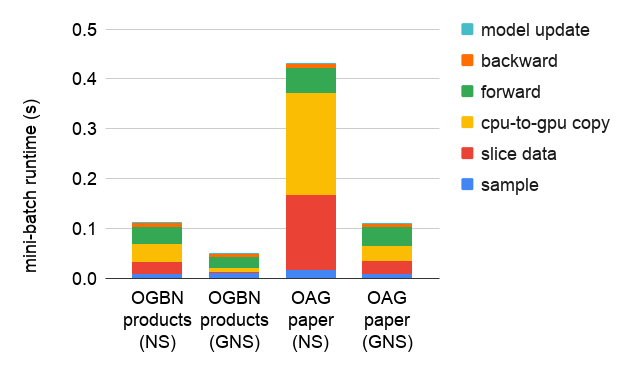
Figure 2. Runtime breakdown (s) of each component in mini-batch training of NS and GNS on OGBN-products and OAG-paper graphs.

Table 4. The average number of input nodes in a mini-batch of NS and GNS as well as the average number of input nodes from the cache of GNS.

	#input nodes	#input nodes	#cached nodes
	(NS)	(GNS)	(GNS)
Yelp	151341	24150	5796
Amazon	132288	19063	13986
OGBN-products	433928	88137	21552
OAG-paper	408854	102984	56422
OGBN-Papers100M	507405	155128	111923

We plot the convergence rate of all of the training methods on OGBN-products based on the test F1-scores (Figure 3). In this study, LADIES samples 512 nodes per layer and GNS caches 1% of nodes in the graph. The result indicates that GNS achieves similar convergence and accuracy as NS even with a small cache, thereby confirming the theoretical analysis in Section 3.5, while LADIES and LazyGCN fail to converge to good model accuracy.

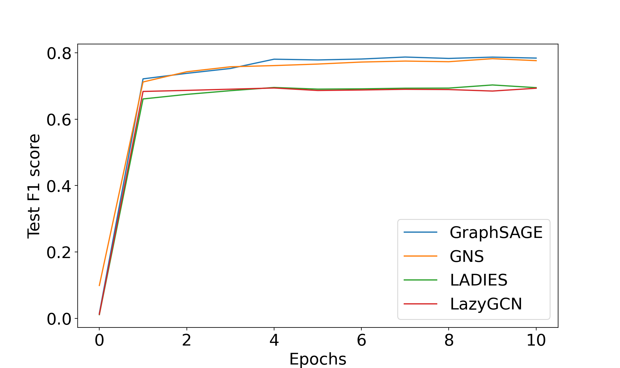
Figure 3. Comparison of the accuracy (F1 score) v.s. epochs.

Table 5. Percentage of isolated training nodes in LADIES.

# of sampled nodes/layer	256	512	1000	5000	10000
% of isolated target nodes	52.7	45.2	24.0	3.9	0

Percentage of isolated nodes in the first layer when training three-layer GCN on OGBN-products with LADIES.

One of reasons why LADIES suffers poor performance is that it tends to construct a mini-batch with many isolated nodes, especially for nodes in the first layer (Table 5). When training three-layer GCN on OGBN-products with LADIES, the percentage of isolated nodes in the first layer under different numbers of layerwise sampled nodes is illustrated in Tables 5.

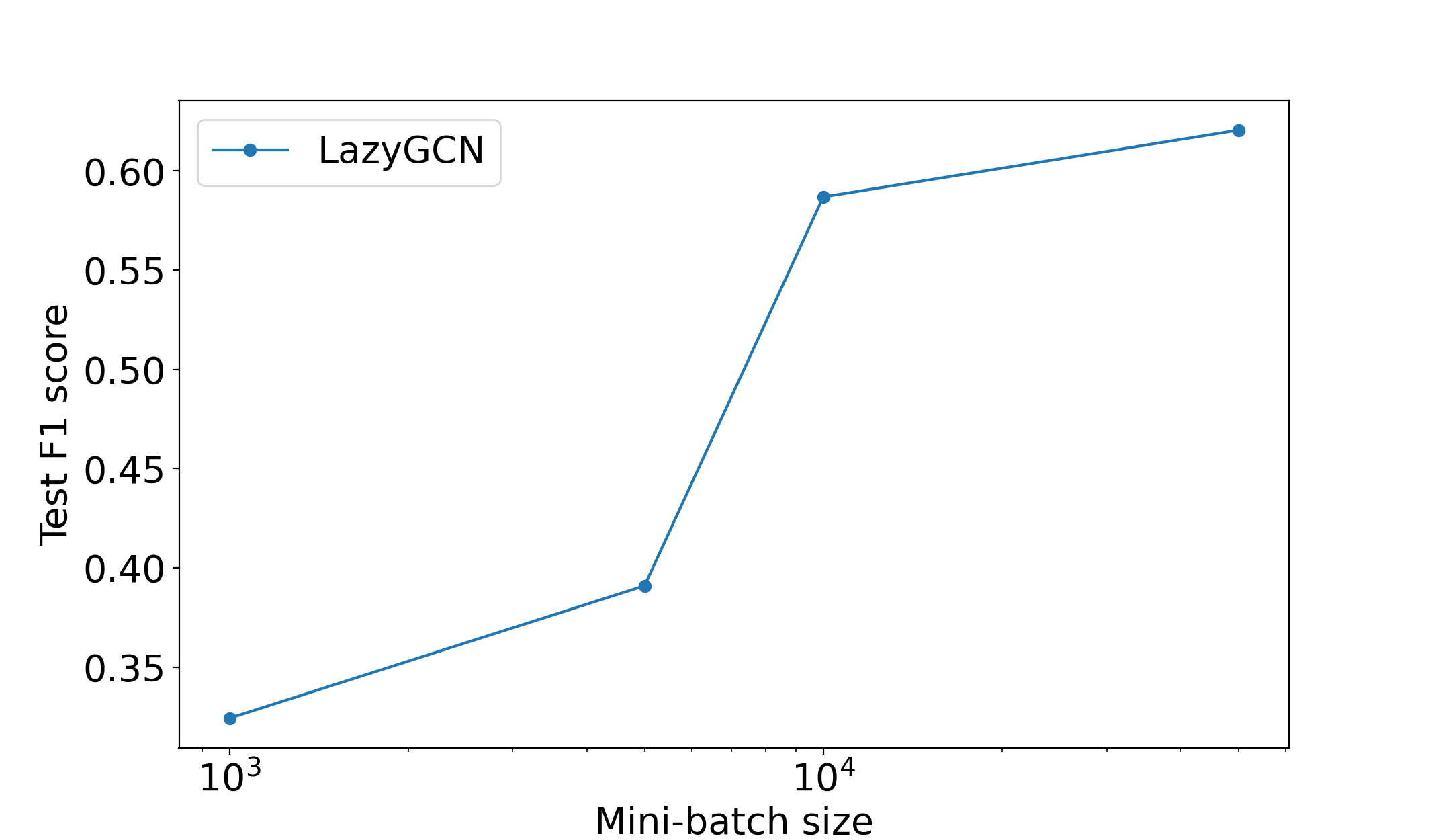
Figure 4. The effect of mini-batch size on the performance of LazyGCN on the Yelp dataset.

LazyGCN requires a large batch size to train GCN on large graphs, which usually leads to out of memory. Under the same setting of the paper (Ramezani et al., 2020), we investigate the performance of nodewise lazyGCN on Yelp dataset with different mini-batch sizes. As shown in Figure 4, LazyGCN performs poorly at the small mini-batch size. This may be caused by training with less representative graph data in mega-batch when recycling a small batch.

4.3. Hyperparameter study

In this section, we explore the effect of various parameters in GNS on OGBN-products dataset. Table 6 summarizes the test F1-score with respect to different values of cache update period sizes $P$ and cache sizes. A cache size as small as $0.01\%$ can still achieve a fairly good accuracy. As long as the cache size is sufficiently large (e.g., $1\%\cdot|\mathcal{V}|$), properly reducing the frequency of updating the cache (e.g., $P=1,2,5$) does not affect performance. Note that it is better to get a $.1\%$ sample every epoch, than a single $1\%$ sample every 10 epochs, and $.01\%$ sample every epoch that the $0.1\%$ sample every 10 epochs.

Table 6. GNS sensitivity to update period and cache size.

	cache update period size $P$
Size of cache	$P=1$	$P=2$	$P=5$	$P=10$
$|\mathcal{V}|\times 1\%$	78.34	78.40	78.17	77.54
$|\mathcal{V}|\times.1\%$	78.04	77.31	76.16	74.71
$|\mathcal{V}|\times.01\%$	76.29	72.83	71.60	71.21

Performance in terms of test-set F1-score for different cache sizes and update periods.

5. Conclusions

In this paper, we propose a new effective sampling framework to accelerate GNN mini-batch training on giant graphs by removing the main bottleneck in mixed CPU-GPU training. GNS creates a global cache to facilitate neighbor sampling and periodically updates the cache. Therefore, it reduces data movement between CPU and GPU. We empirically demonstrate the advantages of the proposed algorithm in convergence rate, computational time, and scalability to giant graphs. Our proposed method has a significant speedup in training on large-scale dataset. We also theoretically analyze GNS and show that even with a small cache size, it enjoys a comparable convergence rate as the node-wise sampling method.

Appendix A Proof of Theorem 1

By extending Lemma 4 in (Ramezani et al., 2020), we conclude that $\mathbb{E}[\|\nabla J(\hat{\bm{\theta}})\|^{2}]$ depends on $\frac{1}{T}\sum_{t=1}^{T}\mathbb{E}[\|\nabla\widetilde{J}_{\mathcal{B}}(\bm{\theta}_{t})-\nabla J(\bm{\theta}_{t})\|^{2}]$. To complete the proof of theorem 1, we first present few vital lemmas. To be specific, Lemma 1 characterizes the bounds on $\frac{1}{T}\sum_{t=1}^{T}$ $\mathbb{E}[\|\nabla\widetilde{J}_{\mathcal{B}}(\bm{\theta}_{t})-\nabla J(\bm{\theta}_{t})\|^{2}]$.

Lemma 0.

Denote $N^{i}_{\ell}$ as the number of the neighborhood nodes with respect to $i\in\mathcal{V}$ sampling uniformly at random at $\ell$-th layer. The cached nodes in the set $\mathcal{C}$ with the size of $|\mathcal{C}|$ are sampled without replacement according to $p^{\text{cache}}_{v}$. The dimension of node feature is denoted as $n$ and the size of min-batch is denoted as $B$. Define $\widetilde{C}=|\mathcal{C}|/|\mathcal{V}|$ and $C_{d}=\sum_{v_{i}\in\mathcal{V}}\mathrm{deg}(v_{i})/|\mathcal{V}|$ with the constant $c>0$. Under Assumption 1, the expected mean-square error of stochastic gradient $\nabla\widetilde{J}_{\mathcal{B}}(\bm{\theta})$ derived from Algorithm 1 to the full gradient is bounded by

$$\mathrm{MSE}:=\frac{1}{T}\sum_{t=1}^{T}\mathbb{E}\left[\left\|\nabla\widetilde{J}_{\mathcal{B}}(\bm{\theta}_{t})-\nabla J(\bm{\theta}_{t})\right\|^{2}\right]$$

$$\leq \mathcal{O}\left(L^{{}^{\prime}2}_{f}\frac{\log(4n/\delta)+1/2}{B}\right)+\mathcal{O}\left(L_{f}^{{}^{\prime}2}L_{g}^{4}\frac{\log(4n/\delta)+1/2}{c\widetilde{C}C_{d}N_{1}^{j}N_{2}^{i}}\right)$$

(A.1) $$+\mathcal{O}\left(L_{g}^{{}^{\prime}2}L_{f}^{2}\frac{\log(4n/\delta)}{c\widetilde{C}C_{d}N_{1}^{j}N_{2}^{i}}\right).$$

Proof.

According to the inequality, $\|\bm{a}+\bm{b}\|^{2}\leq 2\|\bm{a}\|^{2}+2\|\bm{b}\|^{2}$, $\mathrm{MSE}$ (1) can be decomposed into two parts:

$$\mathrm{MSE}:=\frac{1}{T}\sum_{t=1}^{T}\mathbb{E}\left[\left\|\nabla\widetilde{J}_{\mathcal{B}}(\bm{\theta}_{t})-\nabla J(\bm{\theta}_{t})\right\|^{2}\right]$$

$$\leq \frac{2}{T}\sum_{t=1}^{T}\mathbb{E}\left[\left\|\nabla\widetilde{J}_{\mathcal{B}}\left(\bm{\theta}_{t}\right)-\nabla J_{\mathcal{B}}\left(\bm{\theta}_{t}\right)\right\|^{2}\right]$$

(A.2) $$+\frac{2}{T}\sum_{t=1}^{T}{\mathbb{E}\left[\left\|\nabla J_{\mathcal{B}}\left(\bm{\theta}_{t}\right)-\nabla J\left(\bm{\theta}_{t}\right)\right\|^{2}\right]}$$

Two terms in (A) are bounded by Lemma 2 and 3, respectively. ∎

Lemma 0.

Based on the notations in Lemma 1, with probability exceeding $1-\delta$ we have

$$\mathbb{E}[\|\nabla\widetilde{J}_{\mathcal{B}}(\bm{\theta})-\nabla J_{\mathcal{B}}(\bm{\theta})\|^{2}]$$

(A.3) $$\leq 128L_{f}^{{}^{\prime}2}L_{g}^{4}\frac{\log(4n/\delta)+1/2}{c\widetilde{C}C_{d}N_{1}^{j}N_{2}^{i}}+64L_{g}^{{}^{\prime}2}L_{f}^{2}\frac{\log(4n/\delta)}{c\widetilde{C}C_{d}N_{1}^{j}N_{2}^{i}}.$$

Proof.

The proof of Lemma 2 is provided in Appendix B. ∎

Lemma 0.

Based on the notations in Lemma 1, with probability exceeding $1-\delta$ we have

(A.4) $$\mathbb{E}[\|\nabla{J}_{\mathcal{B}}(\bm{\theta})-\nabla J(\bm{\theta})\|^{2}]\leq 128L_{f}^{{}^{\prime}2}\frac{\log(4n/\delta)+1/2}{B}.$$

Proof.

Besides the definition of $\nabla J_{\mathcal{B}}(\bm{\theta})$ (B.1), $\nabla J(\bm{\theta})$ is given as

(A.5) $$\nabla J(\bm{\theta})=\frac{1}{|\mathcal{V}|}\sum_{i\in\mathcal{V}}A_{1}^{i}A_{2}^{i},$$

where $A_{1}^{i},A_{2}^{i}$ are represented by (B.2) and (B.3), respectively.

For simplicity,we denote

$$\mathbb{E}_{\mathcal{V}_{\mathcal{B}}\sim\mathcal{V}}\big{[}\mathbb{E}_{j\sim\mathcal{N}(i),\forall i\in\mathcal{V}_{\mathcal{B}}}[\mathbb{E}_{k\sim\mathcal{N}(j),\forall j\in\mathcal{N}(i)}[\cdot]]\big{]}$$

as $\mathbb{E}[\cdot]$.

(A.6) $$\mathbb{E}[\|\nabla{J}_{\mathcal{B}}(\bm{\theta})-\nabla J(\bm{\theta})\|^{2}]$$

(A.7) $$\leq \mathbb{E}\left[\left\|\frac{1}{B}\sum_{i\in\mathcal{V}_{\mathcal{B}}}A_{1}^{i}A_{2}^{i}-\frac{1}{|\mathcal{V}|}\sum_{i\in\mathcal{V}}A_{1}^{i}A_{2}^{i}\right\|^{2}\right],$$

(A.8) $$\leq 128L_{f}^{{}^{\prime}2}\frac{\log(4n/\delta)+1/2}{c\widetilde{C}C_{d}N_{1}^{j}N_{2}^{i}},$$

where the last inequality comes from Lemma 1. ∎

Appendix B Proof of Lemma 2

To bound $\mathbb{E}[\|\nabla\widetilde{J}_{\mathcal{B}}(\bm{\theta})-\nabla J_{\mathcal{B}}(\bm{\theta})\|^{2}]$, we begin with the definition of $\nabla\widetilde{J}_{\mathcal{B}}(\bm{\theta})$ and $\nabla J_{\mathcal{B}}(\bm{\theta}){}$, which is given by

(B.1) $$\nabla J_{\mathcal{B}}(\bm{\theta})=\frac{1}{B}\sum_{i\in\mathcal{V}_{\mathcal{B}}}A_{1}^{i}A_{2}^{i},$$

where

(B.2) $$A_{1}^{i} =\nabla f_{i}\left(\frac{1}{|\mathcal{N}(i)|}\sum_{j\in\mathcal{N}(i)}\frac{1}{|\mathcal{N}(j)|}\sum_{k\in\mathcal{N}(j)}g_{jk}(\bm{\theta})\right),$$

(B.3) $$A_{2}^{i} =\frac{1}{|\mathcal{N}(i)|}\sum_{j\in\mathcal{N}(i)}\frac{1}{|\mathcal{N}(j)|}\sum_{k\in\mathcal{N}(j)}\nabla g_{jk}(\bm{\theta}).$$

(B.4) $$\nabla\widetilde{J}_{\mathcal{B}}(\bm{\theta})=\frac{1}{B}\sum_{i\in\mathcal{V}_{\mathcal{B}}}B_{1}^{i}B_{2}^{i}$$

where

(B.5) $$B_{1}^{i} =\nabla f_{i}\left(\frac{1}{|\mathcal{N}_{2}^{\mathcal{C}}(i)|}\sum_{j\in\mathcal{N}_{2}^{\mathcal{C}}(i)}\frac{1}{|\mathcal{N}_{1}^{\mathcal{C}}(j)|}\sum_{k\in\mathcal{N}_{1}^{\mathcal{C}}(j)}p_{k}^{(1)}g_{jk}(\bm{\theta})\right),$$

(B.6) $$B_{2}^{i} =\frac{1}{|\mathcal{N}_{2}^{\mathcal{C}}(i)|}\sum_{j\in\mathcal{N}_{2}^{\mathcal{C}}(i)}\frac{1}{|\mathcal{N}_{1}^{\mathcal{C}}(j)|}\sum_{k\in\mathcal{N}_{1}^{\mathcal{C}}(j)}p_{k}^{(1)}\nabla g_{jk}(\bm{\theta}).$$

For simplicity,we denote

$$\mathbb{E}_{\mathcal{V}_{\mathcal{B}}\sim\mathcal{V}}\left[\mathbb{E}_{j\sim\mathcal{N}(i),\forall i\in\mathcal{V}_{\mathcal{B}}}[\mathbb{E}_{k\sim\mathcal{N}(j),\forall j\in\mathcal{N}(i)}[\cdot]]\right]$$

as $\mathbb{E}[\cdot]$.

Based on the inequalities $\left\|\frac{1}{n}\sum_{i=1}^{n}\bm{a}_{i}\right\|\leq\frac{1}{n}\sum_{i=1}^{n}\left\|\bm{a}_{i}\right\|$, $\|\bm{a}+\bm{b}\|^{2}\leq$ $2\|\bm{a}\|+2\|\bm{b}\|,$ and $\|\bm{ab}\|\leq\|\bm{a}\|\|\bm{b}\|$, we arrive

$$\mathbb{E}[\|\nabla\widetilde{J}_{\mathcal{B}}(\bm{\theta})-\nabla J_{\mathcal{B}}(\bm{\theta})\|^{2}]$$

$$= 2\mathbb{E}\left[\left\|B_{1}^{i}\right\|^{2}\right]\mathbb{E}\left[\left\|B_{2}^{i}-A_{2}^{i}\right\|^{2}\right]$$

(B.7) $$+2\mathbb{E}\left[\left\|B_{1}^{i}-A_{1}^{i}\right\|^{2}\right]\mathbb{E}\left[\left\|A_{2}^{i}\right\|^{2}\right].$$

We shall bound two terms in (B.7).

1. The first term: for $\mathbb{E}\left[\left\|B_{1}^{i}\right\|^{2}\right]$, we have

   (B.8) $$\mathbb{E}\left[\left\|B_{1}^{i}\right\|^{2}\right]\leq L_{f}^{2}.$$

   In terms of $\mathbb{E}\left[\left\|B_{2}^{i}-A_{2}^{i}\right\|^{2}\right]$, we have

   $$\mathbb{E}\left[\left\|B_{2}^{i}-A_{2}^{i}\right\|^{2}\right]$$

   $$= L_{f}^{{}^{\prime}2}\mathbb{E}\Bigg{[}\bigg{\|}\sum_{j\in\mathcal{N}_{2}^{\mathcal{C}}(i)}\sum_{k\in\mathcal{N}_{1}^{\mathcal{C}}(j)}\frac{p_{k}^{(1)}}{N_{\mathcal{C}_{2}}^{i}N_{\mathcal{C}_{1}}^{j}}\nabla g_{jk}(\bm{\theta})$$

   $$- \sum_{j\in\mathcal{N}(i)}\sum_{k\in\mathcal{N}(j)}\frac{1}{(N^{i})^{2}}\nabla g_{jk}(\bm{\theta})\bigg{\|}^{2}\Bigg{]}$$

   (B.9) $$\leq 64L_{g}^{{}^{\prime}2}\frac{\log(4n/\delta)}{c\widetilde{C}C_{d}N_{1}^{j}N_{2}^{i}},$$

   where the last inequality comes from Lemma 1.

2. The second term: for $\mathbb{E}\left[\left\|A_{2}^{i}\right\|^{2}\right]$, we have

   (B.10) $$\mathbb{E}\left[\left\|A_{2}^{i}\right\|^{2}\right]\leq L_{g}^{2}.$$

   In terms of $\mathbb{E}\left[\left\|B_{1}^{i}-A_{1}^{i}\right\|^{2}\right]$, we have

   $$\mathbb{E}\left[\left\|B_{1}^{i}-A_{1}^{i}\right\|^{2}\right]$$

   $$= L_{f}^{{}^{\prime}2}\mathbb{E}\Bigg{[}\bigg{\|}\sum_{j\in\mathcal{N}_{2}^{\mathcal{C}}(i)}\sum_{k\in\mathcal{N}_{1}^{\mathcal{C}}(j)}\frac{p_{k}^{(1)}}{N_{\mathcal{C}_{2}}^{i}N_{\mathcal{C}_{1}}^{j}}g_{jk}(\bm{\theta})$$

   $$- \sum_{j\in\mathcal{N}(i)}\sum_{k\in\mathcal{N}(j)}\frac{1}{(N^{i})^{2}}g_{jk}(\bm{\theta})\bigg{\|}^{2}\Bigg{]}$$

   (B.11) $$\leq 128L_{g}^{2}L_{f}^{{}^{\prime}2}\frac{\log(4n/\delta)+1/2}{c\widetilde{C}C_{d}N_{1}^{j}N_{2}^{i}},$$

   where the last inequality comes from Lemma 1.

By integrating inequalities (B.8), (B.11), (B.10), (B.9), it yields

$$\mathbb{E}[\|\nabla\widetilde{J}_{\mathcal{B}}(\bm{\theta})-\nabla J_{\mathcal{B}}(\bm{\theta})\|^{2}]$$

(B.12) $$\leq 128L_{f}^{{}^{\prime}2}L_{g}^{4}\frac{\log(4n/\delta)+1/2}{c\widetilde{C}C_{d}N_{1}^{j}N_{2}^{i}}+64L_{g}^{{}^{\prime}2}L_{f}^{2}\frac{\log(4n/\delta)}{c\widetilde{C}C_{d}N_{1}^{j}N_{2}^{i}}.$$

Lemma 0.

Based on the notations in Lemma 1, with probability $1-\delta$ we have

$$\mathbb{E}\Bigg{[}\bigg{\|}\sum_{j\in\mathcal{N}_{2}^{\mathcal{C}}(i)}\sum_{k\in\mathcal{N}_{1}^{\mathcal{C}}(j)}\frac{p_{k}^{(1)}}{N_{\mathcal{C}_{2}}^{i}N_{\mathcal{C}_{1}}^{j}}g_{jk}(\bm{\theta})$$

$$-\mathbb{E}_{j\sim\mathcal{N}(i),k\sim\mathcal{N}(j)}[g_{jk}(\bm{\theta})]\bigg{\|}^{2}\Bigg{]}$$

(B.13) $$\leq 8\sqrt{2}L_{g}\sqrt{\frac{\log(4n/\delta)+1/2}{c\widetilde{C}C_{d}N_{1}^{j}N_{2}^{i}}}\quad\forall~{}i\in\mathcal{V}$$

$$\mathbb{E}\Bigg{[}\bigg{\|}\sum_{j\in\mathcal{N}_{2}^{\mathcal{C}}(i)}\sum_{k\in\mathcal{N}_{1}^{\mathcal{C}}(j)}\frac{p_{k}^{(1)}}{N_{\mathcal{C}_{2}}^{i}N_{\mathcal{C}_{1}}^{j}}\nabla g_{jk}(\bm{\theta})$$

$$-\mathbb{E}_{j\sim\mathcal{N}(i),k\sim\mathcal{N}(j)}[\nabla g_{jk}(\bm{\theta})]\bigg{\|}^{2}\Bigg{]}$$

(B.14) $$\leq 8L^{\prime}_{g}\sqrt{\frac{\log(4n/\delta)}{c\widetilde{C}C_{d}N_{1}^{j}N_{2}^{i}}}\quad\forall~{}i\in\mathcal{V},$$

where $C_{d}=\sum_{v_{i}\in\mathcal{V}}\mathrm{deg}(v_{i})/|\mathcal{V}|$ with the constant $c>0$.

Proof.

The proof is derived from the proof of Lemma 6 in (Kohler and Lucchi, 2017) and Lemma 10 and 11 in (Ramezani et al., 2020). Based on the definition of $p_{k}^{(1)}$, for $i\in\mathcal{V}$, we have

$$\mathbb{E}\left[\sum_{j\in\mathcal{N}_{2}^{\mathcal{C}}(i)}\sum_{k\in\mathcal{N}_{1}^{\mathcal{C}}(j)}\frac{p_{k}^{(1)}}{N_{\mathcal{C}_{2}}^{i}N_{\mathcal{C}_{1}}^{j}}g_{jk}(\bm{\theta})\right]$$

(B.15) $$= \mathbb{E}_{j\sim\mathcal{N}(i),k\sim\mathcal{N}(j)}[g_{jk}(\bm{\theta})].$$

Similarly, there is

$$\mathbb{E}\left[\sum_{j\in\mathcal{N}_{2}^{\mathcal{C}}(i)}\sum_{k\in\mathcal{N}_{1}^{\mathcal{C}}(j)}\frac{p_{k}^{(1)}}{N_{\mathcal{C}_{2}}^{i}N_{\mathcal{C}_{1}}^{j}}\nabla g_{jk}(\bm{\theta})\right]$$

(B.16) $$= \mathbb{E}_{j\sim\mathcal{N}(i),k\sim\mathcal{N}(j)}[\nabla g_{jk}(\bm{\theta})].$$

The value of $N_{\mathcal{C}_{1}}^{j}$ and $N_{\mathcal{C}_{2}}^{j}$ depend on the predefined number of neighborhood nodes sampled uniformly at random in each layer, i.e., $N_{2}^{i},N_{1}^{j}$, the ratio of cached nodes to the whole graph nodes, i.e., $\widetilde{C}=|\mathcal{C}|/|\mathcal{V}|$ and the sampling probability $\mathcal{P}$. Thus, $N_{\mathcal{C}_{1}}^{j}$ can be approximated by $N_{\mathcal{C}_{1}}^{j}=c\widetilde{C}C_{d}N_{1}^{j}$ where $C_{d}=\sum_{v_{i}\in\mathcal{V}}\mathrm{deg}(v_{i})/|\mathcal{V}|$ with the constant $c>0$. Based on the above, the proof can be completed by extending the proof of Lemma 10 and 11 in (Ramezani et al., 2020).

Given the sampled set $\mathcal{S}_{1},\mathcal{S}_{2}$ and

$$V_{S}(\bm{\theta})=\frac{1}{|S_{1}|\cdot|S_{2}|}\sum_{i\in\mathcal{S}_{1}}\sum_{j\in\mathcal{S}_{2}}V_{ij}(\bm{\theta}),$$

where $V_{ij}(\bm{\theta})\in\mathbb{R}^{n}$ is $L_{v}$-Lipschitz continuous for all $i,j$, the proof can be completed via Bernstein’s bound with a sub-Gaussian tail, given by we have

$$\mathbb{P}\left(\left\|V_{S}(\bm{\theta})-\mathbb{E}[V_{S}(\bm{\theta})]\right\|\geq\epsilon\right)$$

(B.17) $$\leq 4n\cdot\exp\left(-\frac{\epsilon^{2}|S_{1}|\cdot|S_{2}|}{64L_{v}^{2}}+\frac{1}{2}\right),$$

where $\epsilon\leq 2L_{v}$.

Finally, let $\delta$ as the upper bound of Bernstein inequality

(B.18) $$\delta=4n\cdot\exp\left(-\frac{\epsilon^{2}|S_{1}|\cdot|S_{2}|}{64L_{v}^{2}}+\frac{1}{2}\right).$$

Therefore, we have

(B.19) $$\epsilon=8\sqrt{2}L_{v}\sqrt{\frac{\log(4n/\delta)+1/2}{|S_{1}|\cdot|S_{2}|}}.$$

The inequality (B.14) can be clarified in similar way. ∎

References

- (1)
- Chen et al. (2018) Jie Chen, Tengfei Ma, and Cao Xiao. 2018. FastGCN: Fast Learning with Graph Convolutional Networks via Importance Sampling. In 6th International Conference on Learning Representations, ICLR 2018, Vancouver, BC, Canada, April 30 - May 3, 2018, Conference Track Proceedings. https://openreview.net/forum?id=rytstxWAW
- Devlin et al. (2019) Jacob Devlin, Ming-Wei Chang, Kenton Lee, and Kristina Toutanova. 2019. BERT: Pre-training of Deep Bidirectional Transformers for Language Understanding. abs/1810.04805 (2019).
- Fey and Lenssen (2019) Matthias Fey and Jan Eric Lenssen. 2019. Fast Graph Representation Learning with PyTorch Geometric. CoRR abs/1903.02428 (2019).
- Hamilton et al. (2017) William L. Hamilton, Zhitao Ying, and Jure Leskovec. 2017. Inductive Representation Learning on Large Graphs. In Advances in Neural Information Processing Systems 30: Annual Conference on Neural Information Processing Systems 2017, 4-9 December 2017, Long Beach, CA, USA. 1025–1035. http://papers.nips.cc/paper/6703-inductive-representation-learning-on-large-graphs
- Hochreiter and Schmidhuber (1997) Sepp Hochreiter and Jürgen Schmidhuber. 1997. Long short-term memory. Neural computation 9, 8 (1997), 1735–1780.
- Hu et al. (2020) Weihua Hu, Matthias Fey, Marinka Zitnik, Yuxiao Dong, Hongyu Ren, Bowen Liu, Michele Catasta, and Jure Leskovec. 2020. Open graph benchmark: Datasets for machine learning on graphs. arXiv preprint arXiv:2005.00687 (2020).
- Kipf and Welling ([n. d.]) Thomas N. Kipf and Max Welling. [n. d.]. Semi-Supervised Classification with Graph Convolutional Networks. In 5th International Conference on Learning Representations (ICLR-17).
- Kohler and Lucchi (2017) Jonas Moritz Kohler and Aurelien Lucchi. 2017. Sub-sampled Cubic Regularization for Non-convex Optimization. In International Conference on Machine Learning. 1895–1904.
- Liu et al. (2020) Ziqi Liu, Zhengwei Wu, Zhiqiang Zhang, Jun Zhou, Shuang Yang, Le Song, and Yuan Qi. 2020. Bandit Samplers for Training Graph Neural Networks. abs/2006.05806 (2020).
- Qi et al. (2017) Charles R Qi, Hao Su, Kaichun Mo, and Leonidas J Guibas. 2017. Pointnet: Deep learning on point sets for 3d classification and segmentation. In Proceedings of the IEEE conference on computer vision and pattern recognition. 652–660.
- Ramezani et al. (2020) Morteza Ramezani, Weilin Cong, Mehrdad Mahdavi, Anand Sivasubramaniam, and Mahmut Kandemir. 2020. GCN meets GPU: Decoupling “When to Sample” from “How to Sample”. Advances in Neural Information Processing Systems 33 (2020).
- Tang et al. (2008) Jie Tang, Jing Zhang, Limin Yao, Juanzi Li, Li Zhang, and Zhong Su. 2008. ArnetMiner: Extraction and Mining of Academic Social Networks. In Proceedings of the 14th ACM SIGKDD International Conference on Knowledge Discovery and Data Mining. New York, NY, USA.
- Velickovic et al. ([n. d.]) Petar Velickovic, Guillem Cucurull, Arantxa Casanova, Adriana Romero, Pietro Liò, and Yoshua Bengio. [n. d.]. Graph Attention Networks. In 6th International Conference on Learning Representations (ICLR-18).
- Wang et al. (2019) Minjie Wang, Da Zheng, Zihao Ye, Quan Gan, Mufei Li, Xiang Song, Jinjing Zhou, Chao Ma, Lingfan Yu, Yu Gai, Tianjun Xiao, Tong He, George Karypis, Jinyang Li, and Zheng Zhang. 2019. Deep Graph Library: A Graph-Centric, Highly-Performant Package for Graph Neural Networks. arXiv preprint arXiv:1909.01315 (2019).
- Zeng et al. (2019) Hanqing Zeng, Hongkuan Zhou, Ajitesh Srivastava, Rajgopal Kannan, and Viktor Prasanna. 2019. Graphsaint: Graph sampling based inductive learning method. arXiv preprint arXiv:1907.04931 (2019).
- Zheng et al. (2020) Da Zheng, Chao Ma, Minjie Wang, Jinjing Zhou, Qidong Su, Xiang Song, Quan Gan, Zheng Zhang, and George Karypis. 2020. DistDGL: Distributed Graph Neural Network Training for Billion-Scale Graphs. arXiv preprint arXiv:2010.05337 (2020).
- Zou et al. (2019) Difan Zou, Ziniu Hu, Yewen Wang, Song Jiang, Yizhou Sun, and Quanquan Gu. 2019. Layer-dependent importance sampling for training deep and large graph convolutional networks. In Advances in Neural Information Processing Systems. 11249–11259.