Third-order many-body expansion of OSV-MP2 wavefunction for low-order scaling analytical gradient computation

Abstract

We present a many-body expansion (MBE) formulation and implementation for efficient computation of analytical energy gradients from the orbital-specific-virtual second-order Møllet-Plesset perturbation theory (OSV-MP2) based on our earlier work (Zhou et al. J. Chem. Theory Comput. 2020, 16, 196–210). The third-order MBE(3) expansion of OSV-MP2 amplitudes and density matrices was developed to adopt the orbital-specific clustering and long-range termination schemes, which avoids term-by-term differentiations of the MBE energy bodies. We achieve better efficiency by exploiting the algorithmic sparsity that allows to prune out insignificant fitting integrals and OSV relaxations. With these approximations, the present implementation is benchmarked on a range of molecules that show an economic scaling in the linear and quadratic regimes for computing MBE(3)-OSV-MP2 amplitude and gradient equations, respectively, and yields normal accuracy comparable to the original OSV-MP2 results. The MPI-3-based parallelism through shared memory one-sided communication is further developed for improving parallel scalability and memory accessibility by sorting the MBE(3) orbital clusters into independent tasks that are distributed on multiple processes across many nodes, supporting both global and local data locations in which selected MBE(3)-OSV-MP2 intermediates of different sizes are distinguished and accordingly placed. The accuracy and efficiency level of our MBE(3)-OSV-MP2 analytical gradient implementation is finally illustrated in two applications: we show that the subtle coordination structure differences of mechanically interlocked Cu-catenane complexes can be distinguished when tuning ligand lengths; and the porphycene molecular dynamics reveals the emergence of the vibrational signature arising from softened N-H stretching associated with hydrogen transfer, using an MP2 level of electron correlation and classical nuclei for the first time.

The University of Hong Kong] Department of Chemistry, The University of Hong Kong, Hong Kong SAR, P.R. China

1 INTRODUCTION

Correlated post-Hartree-Fock (post-HF) methods are being advanced rapidly in the past decade for enabling energy computation of large molecules with systematically controlled accuracy. The strategies for ameliorating post-HF complexities are typically based on two main streams: local correlation methods in which the locality¹ or near-sightedness² of electrons is explored within full system in different ways, and fragmentation- or subdomain-based idea of many variants in which the original formidable problem is broken into many smaller pieces of amenable subproblems. The first stream approaches the full solution by compressing the cluster operators of the entire system in various low-order scaling post-HF methods, predominantly the popular second-order Møllet-Plesset (MP2) perturbation ^{3, 4, 5, 6, 7, 8, 9} and coupled-cluster (CC) theory ^{10, 11, 12, 13, 14, 15, 16, 17, 18, 19, 20, 21, 22, 23}, in the local frameworks such as projected atomic orbitals (PAO), ^{10, 11, 12, 13, 14, 19} pair-nature-orbitals (PNOs)^{24, 25, 18, 26, 27, 28} and orbital-specific-virtuals (OSVs) ^{7, 8, 20, 21, 29}. The second stream seeks and combines many subsystem solutions which aim to approximate the original full solution of the energy via truncated $n$-order many-body expansion (MBE($n$))

$$E=\sum_{I}^{N}E_{I}+\sum_{I>J}^{N}\Delta E_{IJ}+\sum_{I>J>K}^{N}\Delta E_{IJK}+\cdots,$$ (1)

with a myriad of prescriptions for the two-, three-, …, $n$-body subsystems and energy corrections in different versions of MBE, sometimes mutually inclusive, when integrated with correlated wavefunction methods, including the divide-and-conquer ^{30, 31, 32}, the incremental scheme, ^{33, 34, 35, 36, 37, 38, 39, 40, 41} the natural linear scaling method^{42, 43}, the cluster-in-molecule, ^{44, 45, 46, 47, 48} the fragment molecular orbital, ^{49, 50, 51, 52} the embedded MBE^{53, 54, 55, 56, 57} and several others ^{58, 59, 60, 61, 62}.

Both streams have been intensively developed in recent years for correlation treatments and become closely related, for targeting previously difficult systems for which energies now can be computed within reasonable accuracy and time, as demonstrated for thousand-atom MP2^{63, 6, 41, 64} and hundred-atom CC ^{22, 65, 66} benchmark works. Moreover, many structural and spectroscopic properties can be also cast as energy derivatives of the MBE eq 1 with respect to a perturbation,

$$\frac{dE}{d\lambda}=\sum_{I}^{N}\frac{dE_{I}}{d\lambda}+\sum_{I>J}^{N}\frac{d\Delta E_{IJ}}{d\lambda}+\sum_{I>J>K}^{N}\frac{d\Delta E_{IJK}}{d\lambda}+\cdots.$$ (2)

This underlies very promising protocol for computing the properties of extended systems at correlated wavefunction level from MP2 to CC using term-by-term numerical or analytical differentiations of eq 2 up to tractable orders. In recent years, successful applications have been highlighted in a number of ab-initio problems involving electric-field derivatives for electric moments^{67, 68}, polarizabilities^{69, 70} and vibrational spectra^{71, 72, 73}, and nuclear gradients for geometry optimizations ^{55, 74, 75, 76, 77} and molecular dynamics (MD) simulations ^{78, 79, 80, 81, 82, 83, 84, 85}. A tremendous variety of these MBE methods for both energies and properties features the fragmentation schemes in which the subsystems are formed by properly and explicitly cutting macromolecule into overlapping or non-overlapping atomic fragments^{86, 87} prior to post-HF. Alternatively interests also focus on designating the subsystems as tractable “bodies” by grouping orbital domains based on the starting HF wavefunction of the supersystem.

Although MBE provides a general skeleton to integrate with arbitrary electronic structure methods, it becomes practically tractable only if the sequences of eq 1 for energies and eq 2 for observables are well converged and terminated at low expansion orders, for instance, $n\leq 3$ aiming for high accuracy. When we consider the cumulative CPU time $t(n)$ as measurement of the needed hardware resource for computing the MBE($n$) up to the order $n$, apparently $t(n)\approx m_{1}\bar{t}_{1}+m_{2}\bar{t}_{2}+\cdots+m_{n}\bar{t}_{n}$ depends on a few factors for a given macromolecule: (1) the number of independent $i$-body subsystems ($m_{i}$); (2) the size of individual subsystem ($N_{i}$) that needs the average CPU time ($\bar{t}_{i}\sim{\cal{O}}(N_{i}^{p})$, e.g., roughly $p=5$ for canonical MP2 and $p=6$ for CCSD); (3) and the orbital topology belonging to each subsystem which is usually determined at the mean-field level and affects the post-HF MBE($n$) convergence at an expansion order $n$. While it is obvious that such a large number of independent computations must be leveraged in efficient massive parallelism, vast hardware costs can be saved in computations for which both $m_{i}$ and $t_{i}$ increase only moderately (e.g., ${\cal{O}}(N)$) with size of macromolecules. By compressing $m_{i}$, the key idea is to compute only a subset of important MBE terms explicitly, usually in the presence of classical electrostatic and/or approximate dispersion potentials that implicitly fold the corrections from the long-range and high-order nonadditive many-body terms. On the other hand, as the sizes $N_{i}$ of subsystems control the cost of each correlated MBE computation, one could think of computations of lower expense for smaller subsystems, which however often pose difficulty in converging MBE errors and may involve an excessively large number of subsystems. It is therefore desirable to combine the MBE with low-scaling local correlation methods by creating and computing the subsystems of compact orbital topology. In recent years, this strategy has been carefully examined in connection with PAO/PNO/OSV virtual space representation for computing energies of large molecular clusters^{88, 66} and also applied to molecular crystals. ^{89, 90, 91, 92}

In this work, we present an MBE extension of these essential ideas to include energy derivatives that will be rewarding macromolecules based on the local OSV-MP2 analytical gradient formulation we recently developed²⁹. It was shown that the formal scaling of canonical MP2 gradient computation was lowered by about 2–3 orders of magnitude using OSV-MP2. Nevertheless, OSV-MP2 gradient computation is still a resource-intensive task compared to energy. One can envisage that when each MBE 1-body (1b) subsystem is inevitably very large, the large 1b subsystems create superlarge 2-body (2b) and 3-body (3b) subsystems which are prohibitively expensive even for low-scaling methods. By realizing that the OSV ansätz provides the inherently compact representation for virtual space that is adapted to a single molecular orbital (MO), this orbital-specific nature makes OSV a convenient choice for deploying an MBE(3) sequence in which very small pieces of OSV-MP2 analytical gradient computations can be performed on minimum subsystems in the spirit of energy incremental scheme^{33, 34}, i.e., by correlating only individual local MO (LMO) for 1b, LMO pair $ij$ for 2b, and LMO triple $ijk$ for 3b at a time, and keeping other electrons inactive. As such, the OSV virtual domain becomes optimal to correlate 1b LMO (i.e., a pair of electrons), and the union of 1b OSVs creates the local domains specific to 2b and 3b LMOs, respectively. We will show that this MBE($3$)-OSV-MP2 approach already converges OSV-MP2 gradients very well for structure and molecular dynamics (MD) simulations compared to canonical results, without resorting to auxiliary embeddings. This avoids the well known complications of implementing and computing the analytical gradient arising from each subsystem’s response of nonfully variational embedding potential due to the changes of other subsystems. More importantly for complex molecules, $m_{1}$ for 1b subsystems exhibits a natural linear growth with respect to macromolecular size, and $m_{2}$ and $m_{3}$ increase as ${\cal{O}}(N)$ when the intrinsic sparsity within 2b and 3b domains is exploited based on the OSV-based metric.

The remaining discussions are organized as follows. Section 2.1 briefly reviews and reformulates the OSV-MP2 analytical gradient theory, and section 2.2 discusses the third-order MBE(3)-OSV-MP2 algorithm and implementation details for parallel gradient computations based on MPI-3 standard. All integrals and their geometric derivatives are computed using the quantum chemistry program package PYSCF⁹³. Sections 3.1 and 3.2 discuss the performance of the MBE(3)-OSV-MP2 implementation by assessing the accuracy, the origin of errors and the parallel efficiency for computing molecular structures and dynamical properties. Finally, in sections 4.1 and 4.2, we illustrate two short MBE(3)-OSV-MP2 applications in determining the subtle structural changes of Cu-Catenane interlocking complex with varying ligand lengths, as well as molecular dynamics simulation showing protonic tautomerization in porphycene molecule.

2 THEORY AND IMPLEMENTATION

2.1 Review of OSV-MP2 Gradient Theory

We briefly discuss a reformulation of OSV-MP2 analytical gradient theory²⁹, which is essential to the implementation of its MBE extension. We adopt the following convention for noting orbitals: $i,j,k,\cdots$ and $a,b,c,\cdots$ represent the occupied LMOs ($\mathbf{C}^{o}$) and canonical virtual MOs $\mathbf{C}^{v}$, respectively; $\bar{\mu}_{k},\bar{\nu}_{k},\bar{\xi}_{k},\cdots$ refer to a set of OSV orbitals specific to the occupied LMO $k$; $p,q,r,\cdots$ and $\alpha,\beta,\cdots$ pertain to generic indices of MOs and atomic orbitals (AOs), respectively. For brevity, the matrix trace operation is denoted by the bra-ket $\braket{\cdots}$. All matrices and elements are signified by bold and italic letters, respectively.

The OSV-MP2 correlation energy $E_{c}$ is computed according to the orbital-invariant Hylleraas Lagrangian,

$$E_{c}=\sum_{ij}\braket{\mathbf{K}_{(ij,ij)}\overline{\mathbf{T}}_{(ij,ij)}}+\braket{\mathbf{R}_{(ij,ij)}\overline{\mathbf{T}}_{(ij,ij)}}$$ (3)

with $\overline{\mathbf{T}}_{(ij,ij)}=2\mathbf{T}_{(ij,ij)}-\mathbf{T}_{(ij,ij)}^{\dagger}$. The Hylleraas energy minimization with respect to the pair amplitudes $\mathbf{T}_{(ij,ij)}$ yields a set of residual equations that must be solved iteratively in the OSV basis,

$$\mathbf{R}_{(ij,ij)}=\mathbf{K}_{(ij,ij)}+\sum_{k}\mathbf{S}_{(ij,ik)}\mathbf{T}_{(ik,ik)}[\delta_{kj}\mathbf{F}_{(ik,ij)}-f_{kj}\mathbf{S}_{(ik,ij)}]+[\delta_{ik}\mathbf{F}_{(ij,kj)}-f_{ik}\mathbf{S}_{(ij,kj)}]\mathbf{T}_{(kj,kj)}\mathbf{S}_{(kj,ij)}.$$ (4)

The pair amplitudes $\mathbf{T}_{(ij,ij)}$, the residual equations $\mathbf{R}_{(ij,ij)}$ and the relevant quantities $\mathbf{A}_{(ij,kl)}$ are manipulated and stored in the OSV basis of highly compressed dimension, by associating each set of compact OSV orbitals $\{\bar{\mu}_{k}\}$ with individual occupied orbital $k$ through one-index transformation from canonical virtuals $\{a\}$

$$\ket{\bar{\mu}_{k}}=\sum_{a}Q_{a\bar{\mu}}^{k}\ket{a},$$ (5)

where the $k$-specific transformation matrix $\mathbf{Q}_{k}$ is determined by taking the orthonormal eigenvector of the MP2 diagonal pair amplitudes $\mathbf{T}_{kk}$ for each $k$,

$$\left[\mathbf{Q}_{k}^{\dagger}\mathbf{T}_{kk}\mathbf{Q}_{k}\right]_{\bar{\mu}_{k}\bar{\nu}_{k}}=\omega_{\bar{\mu}_{k}}\delta_{\bar{\mu}\bar{\nu}},$$ (6)

with the orthonormality $\mathbf{Q}_{k}^{\dagger}\mathbf{Q}_{k}=\mathbf{1}$. The elements $[\mathbf{T}_{kk}]_{ab}=\frac{(ka\rvert kb)}{f_{aa}+f_{bb}-2f_{kk}}$ are computed using the diagonal elements $f_{kk},f_{aa},f_{bb}$ of the Fock matrix. The level of compactness of OSV space is controlled by the column dimension of the vectors $\mathbf{Q}_{k}$ having eigenvalues $\omega_{\bar{\mu}_{k}}$ greater than a cut-off $l_{\text{osv}}$.

In eq 4, we adopt $\mathbf{A}_{(ij,kl)}$ to represent a generic composite matrix in the OSV-concatenated pair domain that must be assembled between $\{\bar{\mu}_{i},\bar{\nu}_{j}\}$ and $\{\bar{\sigma}_{k},\bar{\xi}_{l}\}$ elements. For instance, $\mathbf{K}_{(ij,ij)}$ denotes the OSV two-electron integral assembled from the composition of $(i\bar{\mu}_{i}\rvert j\bar{\nu}_{i})$, $(i\bar{\mu}_{i}\rvert j\bar{\xi}_{j})$, $(i\bar{\sigma}_{j}\rvert j\bar{\nu}_{i})$ and $(i\bar{\sigma}_{j}\rvert j\bar{\xi}_{j})$. $\mathbf{A}_{(ij,kl)}$ can be however conveniently expressed as a projection of $\mathbf{A}$ from the canonical virtual MOs to OSVs basis and is self-adjoint $\mathbf{A}_{(ij,kl)}^{\dagger}=\mathbf{A}_{(kl,ij)}$,

$$\mathbf{A}_{(ij,kl)}=\left({\begin{array}[]{c}\mathbf{Q}_{i}^{\dagger}\\ \mathbf{Q}_{j}^{\dagger}\end{array}}\right)\mathbf{A}\left({\begin{array}[]{cc}\mathbf{Q}_{k}&\mathbf{Q}_{l}\end{array}}\right).$$ (7)

In the OSV-based analytical gradient theory, the OSV derivative of $\mathbf{A}_{(ij,kl)}$ is needed and formulated by employing the OSV relaxation matrix $\mathbf{O}_{k}^{\lambda}$ with respect to a perturbation $\lambda$,

$$\mathbf{A}_{(ij,kl)}^{\{\lambda\}}=\left({\begin{array}[]{cc}\mathbf{O}_{i}^{\dagger\lambda}&\mathbf{0}\\ \mathbf{0}&\mathbf{O}_{j}^{\dagger\lambda}\end{array}}\right)\mathbf{A}_{(ij,kl)}^{0}+\mathbf{A}_{(ij,kl)}^{0}\left({\begin{array}[]{cc}\mathbf{O}_{k}^{\lambda}&\mathbf{0}\\ \mathbf{0}&\mathbf{O}_{l}^{\lambda}\end{array}}\right),$$ (8)

with the curly brackets $\{\}$ specifying the derivatives of OSVs. Only the off-diagonal block of $\mathbf{O}_{k}^{\lambda}$ between the kept and discarded OSV spaces is needed for accounting effective OSV relaxations, which is cast as perturbed nondegenerate eigenvalue problem²⁹, requiring the first derivative of the diagonal pair amplitudes $\mathbf{T}_{kk}$.

The OSV-MP2 correlation energy $E_{c}[\alpha,\mathbf{C}^{o},\mathbf{Q}_{k},\mathbf{T}_{(ij,ij)}]$ can be viewed as a function of a string of variables: atomic orbitals $\alpha,\beta,\cdots$, LMOs $\mathbf{C}^{o}$, OSVs $\mathbf{Q}_{k}$ and pair amplitudes $\mathbf{T}_{(ij,ij)}$. As the amplitudes $\mathbf{T}_{(ij,ij)}$ are variational to Hylleraas $E_{c}$ and make no contribution, the OSV-MP2 energy derivative $E^{\lambda}_{c}=\frac{dE_{c}}{d\lambda}$ can be computed according to the relaxation contributions merely from OSVs ($E^{\{\lambda\}}_{c}$), LMOs ($E^{[\lambda]}_{c}$) and AOs ($E^{(\lambda)}_{c}$) with respect to a geometric perturbation $\lambda$,

$$E^{\lambda}_{c}=E^{\{\lambda\}}_{c}+E^{[\lambda]}_{c}+E^{(\lambda)}_{c}.$$ (9)

The OSV-specific energy gradient $E^{\{\lambda\}}_{c}$ results from the OSV responses of both the residual equations collected in pair intermediates $\mathbf{M}_{ij}$, and the OSV-based integrals in form of $\mathbf{A}_{(ij,ij)}$ for the integrals $\mathbf{K}_{(ij,ij)}$, $\mathbf{F}_{(ij,ij)}$ and $\mathbf{S}_{(ij,ij)}$. The MO-specific $E^{[\lambda]}_{c}$ arises from the LMO relaxation jointly determined by the geometric responses of canonical MOs and the localization function, requiring the solution to the coupled-perturbed HF and the coupled-perturbed localization equation⁹⁴, respectively. In our implementation, their contributions are merged into the OSV-based Z-vector equation. The AO-specific $E^{(\lambda)}_{c}$ simply evaluates the Hylleraas energy expression of eq 3 in terms of two- and one-electron AO derivative integrals, the occupied-occupied block ($D_{ij}$) and OSV-OSV block ($\mathbf{D}_{(ij,ij)}$) of the unrelaxed density matrices.

Combining all three gradient contributions and using the resolution-of-identity (RI) integral approximation, the total OSV-MP2 energy gradient is reformulated in terms of a variety of density matrices together with the AO-derivatives of Fock (${F}_{\alpha\beta}^{(\lambda)}$), overlap (${S}_{\alpha\beta}^{(\lambda)}$), half-transformed 3-center-2-electron (3c2e) integral ($\mathbf{J}_{i}^{(\lambda)}$) matrices,

$$E_{c}^{\lambda}=\braket{[\mathbf{\check{D}}-\mathbf{C}^{o}\mathbf{Z}^{\dagger}\mathbf{C}^{v\dagger}]\mathbf{F^{(\lambda)}}}-\braket{[\mathbf{\check{D}}^{\prime}+\mathbf{C}^{o}\mathbf{Z}^{\dagger}\mathbf{C}^{v\dagger}+\frac{1}{2}\mathbf{C}^{o}\braket{\mathbf{Z^{\dagger}A}}\mathbf{C}^{o\dagger}]\mathbf{S^{(\lambda)}}}+4\braket{\sum_{i}\mathbf{P}^{v}\mathbf{Y}_{i}^{\dagger}\mathbf{J}_{i}^{(\lambda)}}.$$ (10)

As seen here, the first two trace terms account for the effective one-electron response and the last term for the two-electron response. The one-electron response results eventually from the internal-external orbital rotation by OSV-MP2 Z-vector $\mathbf{Z}$ as well as collective density matrices $\mathbf{\check{D}}$ and $\mathbf{\check{D}}^{\prime}$ in AO basis. $\mathbf{\check{D}}$ collects the direct sum of the OSV overlap-weighted external and internal density matrices ($\mathbf{D}^{v}$ and $\mathbf{D}^{o}$) in the MO basis,

$$\mathbf{\check{D}} = 2\left(\mathbf{C}^{o}~{}\mathbf{C}^{v}\right)\left[\mathbf{D}^{o}\oplus\mathbf{D}^{v}\right]\left(\mathbf{C}^{o}~{}\mathbf{C}^{v}\right)^{\dagger}$$ (11)

with overlap-weighted density matrices in the MO basis,

$$\mathbf{D}^{v} = \sum_{ij}\left(\mathbf{Q}_{i}~{}\mathbf{Q}_{j}\right)\mathbf{D}_{(ij,ij)}\left(\mathbf{Q}_{i}~{}\mathbf{Q}_{j}\right)^{\dagger}+\sum_{ij}\mathbf{T}_{ii}\mathbf{X}_{ij},$$ (12)

$${D}^{o}_{ij} = -D_{ij}-\delta_{ij}\braket{\mathbf{T}_{ii}\sum_{k}\mathbf{X}_{ik}}.$$ (13)

Above, $\mathbf{D}^{v}$ and $\mathbf{D}^{o}$ are composed of the unrelaxed and relaxed contributions. $\mathbf{X}_{ij}$ is an important intermediate resembling the relaxed amplitudes in the MO basis, which accounts for the geometric OSV relaxations of two-electron integrals and residuals, computed in terms of $\mathbf{N}_{ij}$ for the pair $ij$,

$$\mathbf{N}_{ij}=\overline{\mathbf{T}}_{(ij,ij)}\mathbf{K}_{(ij,ij)}+\mathbf{D}_{(ij,ij)}\mathbf{F}_{(ij,ij)}+\mathbf{D}_{(ij,ij)}^{\prime}\mathbf{S}_{(ij,ij)}-\sum_{k}\left[f_{jk}\mathbf{D}_{(ij,ik)}\mathbf{S}_{(ik,ij)}+f_{ik}\mathbf{D}_{(ij,kj)}\mathbf{S}_{(kj,ij)}\right],$$ (14)

where the overlap- ($\mathbf{D}_{(ij,kl)}$) and energy-weighted ($\mathbf{D}_{(ij,kl)}^{\prime}$) density matrices in the OSV basis are,

$$\mathbf{D}_{(ij,kl)} = \frac{1}{2}\left[\overline{\mathbf{T}}_{(ij,ij)}\mathbf{S}_{(ij,kl)}\mathbf{T}_{(kl,kl)}+\overline{\mathbf{T}}_{(ij,ij)}^{\dagger}\mathbf{S}_{(ij,kl)}\mathbf{T}_{(kl,kl)}^{\dagger}\right],$$ (15)

$$\mathbf{D}_{(ij,kl)}^{\prime} = \frac{1}{2}\left[\overline{\mathbf{T}}_{(ij,ij)}\mathbf{F}_{(ij,kl)}\mathbf{T}_{(kl,kl)}+\overline{\mathbf{T}}_{(ij,ij)}^{\dagger}\mathbf{F}_{(ij,kl)}\mathbf{T}_{(kl,kl)}^{\dagger}\right].$$ (16)

Analogously, $\mathbf{\check{D}^{\prime}}$ collects the OSV energy-weighted external contribution ($\mathbf{D}^{\prime v}$), the internal contribution ($\mathbf{D}^{\prime o}$), the HF occupied ($\mathbf{P}^{o}$) and virtual ($\mathbf{P}^{v}$) density matrices for reducing two-electron terms,

$$\mathbf{\check{D}}^{\prime} = 2(\mathbf{C}^{o}~{}\mathbf{C}^{v})[(\mathbf{D}^{\prime o}-\braket{\mathbf{J}_{i}^{\dagger}\mathbf{Y}_{j}\mathbf{P}^{v}})\oplus(\mathbf{D}^{\prime v}-\mathbf{\Lambda}\mathbf{\mathcal{A}})]\left(\mathbf{C}^{o}~{}\mathbf{C}^{v}\right)^{\dagger}$$ (17)

$$+2\sum_{i}\mathbf{P}^{v}(\mathbf{J}_{i}^{\dagger}\mathbf{Y}_{i}\mathbf{P}^{v}-\mathbf{Y}_{i}^{\dagger}\mathbf{J}_{i}\mathbf{P}^{o})$$

with energy-weighted density matrices in the MO basis,

$$\mathbf{D}^{\prime v} = \frac{\mathbf{F}^{v}\mathbf{D}^{v}+\mathbf{D}^{v}\mathbf{F}^{v}}{2},$$ (18)

$${D}^{\prime o}_{ij} = -\sum_{k}f_{ik}D_{ki}-f_{ij}\braket{\mathbf{T}_{ii}\sum_{j}\mathbf{X}_{ij}}.$$ (19)

The two-electron response associated with $\mathbf{J}_{i}^{(\lambda)}$ in eq 10 is driven by the intermediate $\mathbf{Y}_{i}$

$$\mathbf{Y}_{i}=\sum_{j}\mathbf{J}_{j}\left(\mathbf{\check{Q}}_{i}~{}\mathbf{\check{Q}}_{j}\right)\ \overline{\mathbf{T}}_{(ij,ij)}\left(\mathbf{\check{Q}}_{i}~{}\mathbf{\check{Q}}_{j}\right)^{\dagger}+\mathbf{J}_{i}\mathbf{X}_{ij}.$$ (20)

The remaining vector $\mathbf{\Lambda}$ of eq 17 for Pipek-Mezey localization constraint and the $\mathbf{Z}$ of eq 10 for internal-external rotation is the respective solution to the linear coupled-perturbed localization and OSV Z-vector equation,

$$\mathbf{\mathcal{C}}^{\dagger}\mathbf{\Lambda} = \mathbf{\Gamma}^{\dagger},$$ (21)

$$\mathbf{A}^{\dagger}\mathbf{Z} = \mathbf{W}.$$ (22)

$\mathbf{\Gamma}$ and $\mathbf{W}$ on the right are composed of the elements below, respectively,

$${\Gamma}_{ij} = \mathbf{D}^{\prime o}_{ij}-\braket{\mathbf{J}^{\dagger}_{i}\mathbf{Y}_{j}\mathbf{P}^{v}},$$ (23)

$${W}_{ai} = \braket{\mathbf{P}^{v}\mathbf{Y}_{i}^{\dagger}\mathbf{J}_{a}}+\sum_{j}[\mathbf{Y}_{j}^{\dagger}\mathbf{J}_{j}\mathbf{C}^{o}]_{ai}+2\sum_{kl}{\Lambda}_{kl}\mathcal{B}_{kl,ai}.$$ (24)

The two-electron integrals $\mathbf{A}$ are evaluated with RI approximation,

$$A_{ai,bj}=\delta_{ap}\delta_{ij}(f_{aa}-f_{ii})+4(ai\rvert bj)-(ap\rvert ij)-(aj\rvert bi).$$ (25)

More details of these intermediate quantities in eqs 10–22 can be found in our previous work²⁹.

2.2 MBE(3)-OSV-MP2 Gradient Method and Implementation

2.2.1 MBE(3) partitioning, clustering and expansion

The ability to leverage the OSV-MP2 analytical gradient algorithm for efficient large scale computations is based on an MBE partitioning in which the $N$ LMOs from the HF solution of macromolecule is divided into $m_{1}=N$ 1b subsystems. Each $i$-th 1b subsystem is coined a 1b cluster, which constitutes a small number of prescribed OSVs $\{\bar{\mu}_{i}\}$ that become specific to this 1b cluster by the nature of the generation of OSVs, and correlates a pair of electrons within the excitation manifolds $i\to\{\bar{\mu}_{i}\}$. As such, the size of each 1b cluster remains minimum, enabling very small OSV-MP2 gradient computation, and the length of all $N$ 1b clusters grows naturally linearly with sizes of macromolecule.

The union of two 1b clusters makes a 2b cluster in which two electron pairs are correlated in a combined set of the 1b excitation manifolds $(i,j)\to\{\bar{\mu}_{i}\}\cup\{\bar{\nu}_{j}\}$ specific to this pair $ij$. Although the generic length of 2b clusters scales as $N(N+1)/2$, due to the locality of electron correlations which decrease rapidly with distance, the contributions to OSV-MP2 gradients from many weak 2b clusters which are made of relatively remote 1b clusters can be accurately approximated with negligible costs, as compared to that for strong 2b clusters. As a result, a linear growth of the number of the strong 2b clusters can be anticipated as well, which we will discuss in further section.

In contrast to canonical MP2 theory which deals with canonical 2b interactions rigorously, the OSV-MP2 method demands at least indirect 3b corrections to the local 2b interactions in the presence of other LMOs $k$, as clearly indicated in the residual eq 4. The 3b clusters are composed of an incremental union of three 1b clusters for the excitation manifolds $(i,j,k)\to\{\bar{\mu}_{i}\}\cup\{\bar{\nu}_{j}\}\cup\{\bar{\sigma}_{k}\}$. Nevertheless, these 3b corrections must encompass extremely strong pairwise interactions that are simultaneously present amongst $ijk$ LMOs, and higher MBE orders than 3b can be also safely neglected for OSV-MP2 gradients, which defines the MBE(3)-OSV-MP2 ansätz that terminates the MBE series at the third-order. As a result, a substantial amount of 3b clusters can be discarded for 3b contributions, leading to a linear growth of the 3b cluster length with respect to sizes of macromolecule. We will demonstrate that MBE(3)-OSV-MP2 computation suffices to achieve a similar accuracy to what the direct OSV-MP2 energy and gradients can have with identical OSV cut-off $l_{\text{osv}}$.

The selection and screening schemes of 2b and 3b clusters are essential for lowering costs of expensive OSV-MP2 gradient terms. Here, the 2b and 3b expansions are truncated based on the algorithmic metric between the OSVs associated respectively with each LMO, which avoids caveats from real space measurements. As the locality of LMOs and the compactness of OSVs facilitate an exponential decay of OSV overlap matrix elements with the pair $ij$ separation, the average square norm of the OSV overlap matrix indicates the pairwise interaction strength between $ij$ OSV domains that constitute the 2b cluster

$$s^{\text{2b}}_{ij}=\frac{\sum_{\bar{\mu}\bar{\nu}}\braket{\bar{\mu}_{i}}{\bar{\nu}_{j}}^{2}}{\sqrt{n_{i}n_{j}}}$$ (26)

with $\braket{\bar{\mu}_{i}}{\bar{\nu}_{j}}=\mathbf{Q}_{i}^{\dagger}\mathbf{Q}_{j}$ and $n_{i}$ the total number of OSVs for the $i$-th LMO. Using the relation $n_{i}=\sum_{\bar{\mu}\bar{\nu}}\braket{\bar{\mu}_{i}}{\bar{\nu}_{i}}^{2}$, OSV orthonormality and Cauchy-Schwarz inequality, there must be off-diagonal elements $0\leq s^{\text{2b}}_{ij}\leq 1$ and diagonal elements $s_{ii}=1$. Apparently, the magnitude of $s^{\text{2b}}_{ij}$ exhibits strong dependence on the choice of kept OSVs, for instance, $s^{\text{2b}}_{ij}\to 1$ when the OSV set becomes more complete. This ensures that more strong 2b clusters enclosing important pairwise interactions can be automatically identified and adaptively selected, when it is necessary to employ extended OSVs due to tighter OSV cut-off $l_{\text{osv}}$ or more delocalized nature of orbitals. The selection of 3b clusters which contain the united OSV sets for $ijk$ LMOs is based on the mean of the pairwise metrics $s^{\text{2b}}_{ij}$, $s^{\text{2b}}_{ik}$ and $s^{\text{2b}}_{jk}$ from the respective 2b clusters,

$$s^{\text{3b}}_{ijk}=\frac{1}{3}\left(s^{\text{2b}}_{ij}+s^{\text{2b}}_{ik}+s^{\text{2b}}_{jk}\right).$$ (27)

Given a prescription $l_{\text{2b}}$ and $l_{\text{3b}}$ for choosing 2b and 3b clusters, only those important 2b and 3b clusters with $s^{\text{2b}}_{ij}$ and $s^{\text{3b}}_{ijk}$ exceeding their respective $l_{\text{2b}}$ and $l_{\text{3b}}$ values are kept for explicit OSV-MP2 energy and gradient computations. Nevertheless, since the discarded weak 2b corrections amount to still considerable contributions, swift and accurate long-range 2b corrections are implemented and will be presented in the ensuing section. The MBE(3)-OSV-MP2 computation is therefore virtually controlled through a combination of three simple parameters: $l_{\text{osv}}$, $l_{\text{2b}}$ and $l_{\text{3b}}$ for selection of OSVs, 2b and 3b clusters, respectively. However, $l_{\text{3b}}$ must be large enough, as compared to 2b clusters, to allow only 3b clusters of sufficiently strong pairwise interactions. Compared to canonical reference results, we find that the MBE(3)-OSV-MP2 parameters by $l_{\text{osv}}=10^{-4}$, $l_{\text{2b}}=10^{-2}$ and $l_{\text{3b}}=0.2$ yield correlation energies at accuracy better than $99.95\%$ for small testing molecules and $99.7\%$ for large molecules, and gradient RMSDs (root-mean-square deviation) below $10^{-4}$ au.

A major challenge of implementing MBE(3)-OSV-MP2 gradient theory is that it incurs computations of many AO components on the full scale of macromolecule, if separate MBE(3) gradients in eq 2 are carried out on a term-by-term basis, for instance, by repeatedly evaluating AO-based gradients eq 10 and solving Z-vector eq 22 for each differentiation. It is essential to confer an implementation in which we can perform a nonredundant set of small and rapid MBE(3) computations that are unique to individual 2b and 3b clusters in the OSV basis, and evaluate these AO-driven equations once and for all. The idea is to apply the above MBE(3) partitioning and clustering to selected intermediates with major computational costs, rather than to term-by-term energy gradients. These small pieces are then collected to assemble the one-electron contributions $\mathbf{\check{D}}$ and $\mathbf{\check{D}^{\prime}}$, as well as the two-electron contribution $\mathbf{Y}_{i}$.

We can divide these intermediates into 1b-, 2b- and 3b-specific variables. Apparently, LMOs $\mathbf{C}_{i}$, OSVs $\mathbf{Q}_{i}$, 3c2e AO integrals $\mathbf{J}_{i}$ and derivative integrals $\mathbf{J}_{i}^{\lambda}$ are 1b-specific and usually generated when computing 1b clusters; the OSV overlap $\mathbf{S}_{(ij,ij)}$, the Fock $\mathbf{F}_{(ij,ij)}$, the OSV density matrix $\mathbf{D}_{(ij,ij)}$ and two-electron relaxed amplitudes $\mathbf{X}_{ij}$ are 2b-specific, which are determined explicitly up to 2b clusters in terms of other 2b- and 3b-specific objects; the 3b-specific objects, which exhibit the dependence on the explicit pairwise 2b interactions and meanwhile explicit extra interactions correlating more LMOs beyond the pair, as seen in the OSV-MP2 residual in eq 4 and and its OSV response equations in 14. We therefore applied MBE(3) scheme to the following 3b-specific objects, i.e., the OSV amplitudes $\mathbf{T}_{(ij,ij)}$, the internal density matrix $D_{ij}$ and the intermediate $N_{ij}$ as described using MBE(3) expansion in eqs 28–34 analogous to energy, by which the pairwise density matrices (e.g., $\mathbf{D}_{(ij,ij)}$, $\mathbf{D}^{v}$ and $\mathbf{D}^{\prime v}$, $\mathbf{D}^{o}$ and $\mathbf{D}^{\prime o}$) and two-electron relaxed amplitudes $\mathbf{X}_{ij}$ can be then computed only at 2b level. The following MBE(3) expansion has been developed for the diagonal collective pair amplitudes $\mathbf{T}_{(ii,ii)}$,

$$\mathbf{T}_{(ii,ii)}=\mathbf{T}^{i}_{(ii,ii)}+\sum_{k}\Delta\mathbf{T}^{i,k}_{(ii,ii)}+\sum_{k>l}\Delta\mathbf{T}^{i,k,l}_{(ii,ii)},$$ (28)

$$\Delta\mathbf{{T}}^{i,k}_{(ii,ii)}=\mathbf{{T}}^{i,k}_{(ii,ii)}-\mathbf{T}^{i}_{(ii,ii)},$$ (29)

$$\Delta\mathbf{T}^{i,k,l}_{(ii,ii)}=\mathbf{{T}}^{i,k,l}_{(ii,ii)}-\Delta\mathbf{T}^{i,k}_{(ii,ii)}-\Delta\mathbf{T}^{i,l}_{(ii,ii)}-\mathbf{T}^{i}_{(ii,ii)},$$ (30)

and the off-diagonal collective pair amplitudes $\mathbf{T}_{(ij,ij)}$,

$$\mathbf{T}_{(ij,ij)}=\mathbf{T}^{i,j}_{(ij,ij)}+\sum_{k}\Delta\mathbf{T}^{i,j,k}_{(ij,ij)},$$ (31)

$$\Delta\mathbf{T}^{i,j,k}_{(ij,ij)}=\mathbf{T}^{i,j,k}_{(ij,ij)}-\mathbf{T}^{i,j}_{(ij,ij)},$$ (32)

where $\mathbf{T}^{i,j,k}_{(ij,ij)}$ and $\mathbf{T}^{i,k,l}_{(ii,ii)}$ are solved independently from 3b clusters. For instance, the cluster amplitude $\mathbf{T}^{i,j,k}_{(ij,ij)}$ with the superscript $i,j,k$ is obtained by solving the cluster residual equation $\mathbf{R}^{i,j,k}_{(ij,ij)}$ of the 3b cluster that encloses only $i,j,k$ LMOs and associated OSVs. Similarly, the MBE(3) expansions for $\mathbf{N}_{ij}$ follow

$$\mathbf{N}_{ii}=\mathbf{N}^{i}_{ii}+\sum_{k}\Delta\mathbf{N}^{i,k}_{ii}+\sum_{k>l}\Delta\mathbf{N}^{i,k,l}_{ii},$$ (33)

$$\mathbf{N}_{ij}=\mathbf{N}^{i,j}_{ij}+\sum_{k}\Delta\mathbf{N}^{i,j,k}_{ij}$$ (34)

where $\mathbf{N}^{i,j,k}_{ij}$ is computed according to eq 14 taking only $i,j,k$ LMOs for the $ij$ pair. The MBE(3) expansion is also similarly carried out for $D_{ij}$. The MBE(3) scheme facilitates massive parallel computations of these small increments in eqs 28–34 by distributing independent tasks on many processes, which will be discussed in section 2.2.4.

2.2.2 Correlation scheme for weak 2b clusters

Since the number of full 2b clusters increases quadratically with molecular size, to convert the 2b computations into a practically tractable problem, we choose only a subset of 2b clusters for rigorous OSV-MP2 computations, according to the 2b screening scheme in eq 26. A large number of weak 2b clusters, if all simply omitted, would nevertheless produce a substantial amount of aggregate errors to both correlation energies and gradients, which presents a major obstacle for realizing reliable MBE(3)-OSV-MP2 algorithm on large molecules. However, the convergence of the long-range correlation existing in a weak 2b cluster is asymptotically dominated by direct dispersion rather than charge transfer and exchange correlation components. This family of correlation contributions is typically described by the four subblocks of the cluster amplitudes $\mathbf{T}_{(ij,ij)}$, with distinct excitation classes depicted in Figure 1. The dispersion possesses $\{i\to\bar{\mu}_{i},j\to\bar{\xi}_{j}\}$ double excitations genuinely represented by $\mathbf{T}_{(ij,ij)}$ upper-right block, while the diagonal and the lower-left blocks are responsible for the charge transfer $\{i\to\bar{\mu}_{i},j\to\bar{\nu}_{i}\}$ and exchange $\{i\to\bar{\sigma}_{j},j\to\bar{\nu}_{i}\}$ excitations, respectively.

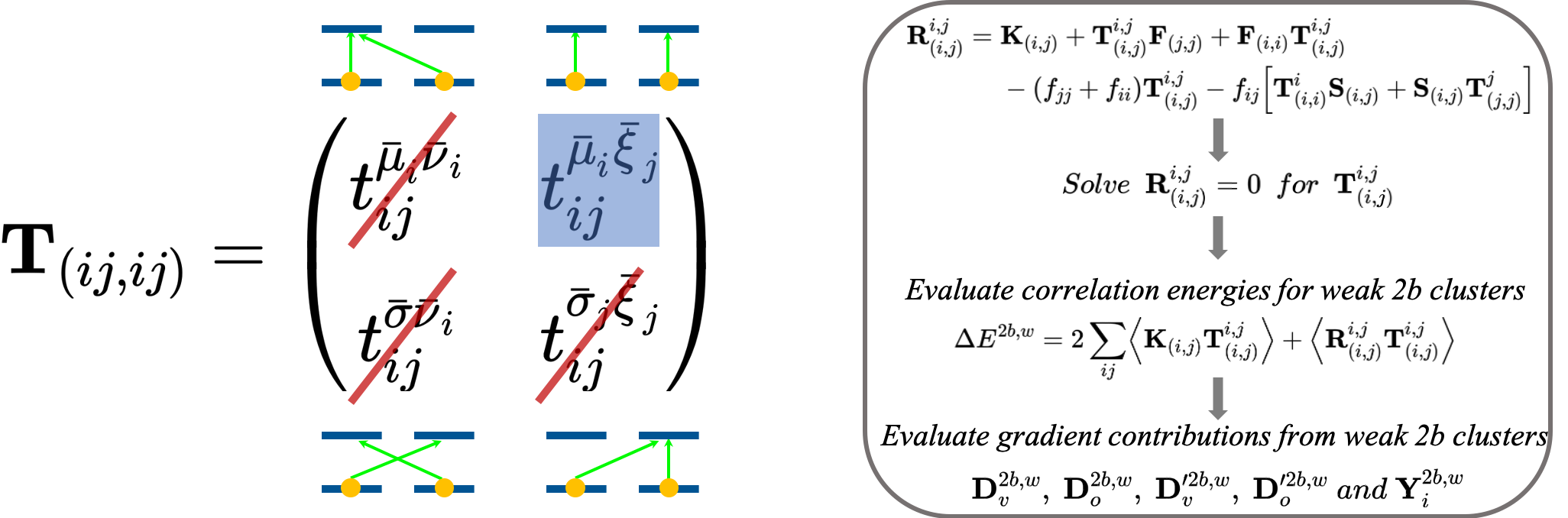
Figure 1: The excitation classes encoded in OSV-MP2 amplitudes (left) and the one-block correlation scheme for treating weak 2b clusters (right).

For the above reasons, we resolve the weak 2b cluster problems by projecting the upper-right block out of the full 2b residual equations, which leads to the one-block algorithm in which the one-block residual equations $\mathbf{R}^{i,j}_{(i,j)}$ are solved for one-block 2b amplitudes $\mathbf{T}^{i,j}_{(i,j)}$, aiming for swiftly capturing direct dispersion. For the gradient contributions from weak 2b clusters, the relevant intermediates of one-block structure of eq 12 are needed. For instance,

$$\mathbf{D}^{v}_{\text{2b},w}=\sum_{ij}\mathbf{Q}_{i}\mathbf{D}_{(i,j)}\mathbf{Q}_{j}^{\dagger}+\sum_{ij}\mathbf{T}_{ii}\mathbf{X}_{ij}^{\text{2b},w}$$ (35)

with one-block overlap- and energy-weighted matrices in the OSV basis,

$$\mathbf{D}_{(i,j)_{w}}=\mathbf{T}^{i,j}_{(i,j)}\mathbf{S}_{(j,i)}\mathbf{T}^{i,j}_{(i,j)}+\mathbf{T}^{\dagger i,j}_{(i,j)}\mathbf{S}_{(j,i)}\mathbf{T}^{\dagger i,j}_{(i,j)},\quad\mathbf{D}^{\prime}_{(i,j)_{w}}=\mathbf{T}^{i,j}_{(i,j)}\mathbf{F}_{(j,i)}\mathbf{T}^{i,j}_{(i,j)}+\mathbf{T}^{\dagger i,j}_{(i,j)}\mathbf{F}_{(j,i)}\mathbf{T}^{\dagger i,j}_{(i,j)}$$ (36)

and the one-block analogue of the residual relaxation is accounted by $\mathbf{X}_{ij}^{\text{2b},w}$. We find that the one-electron part of the residual response in eq 14 makes virtually indiscernible contributions to the total gradient. The insignificance of the one-electron contribution to the residual relaxation results from the small overlap matrix between OSVs residing in the proximity of the remote LMOs that constitute weak 2b clusters. This is demonstrated, for instance, to nonactin molecule for which when 8214 out of 11026 LMO pairs are treated as weak 2b clusters, the OSV-MP2/$l_{\text{osv}}=10^{-4},l_{\text{2b}}=10^{-2}$/def2-tzvp RMSD is only $1.2\times 10^{-5}$ between the gradients with and without one-electron residual relaxation, and the maximum deviation only $8.3\times 10^{-5}$. For reasons of CPU, memory and I/O efficiency, the following approximation is implemented for upper and lower blocks of $\mathbf{N}_{ij}^{\text{2b},w}$, respectively,

$$\left(\mathbf{N}_{ij}^{\text{2b},w}\right)^{\text{up}}\approx\mathbf{T}^{i,j}_{(i,j)}\mathbf{K}_{(j,i)},\quad\left(\mathbf{N}_{ij}^{\text{2b},w}\right)^{\text{low}}\approx 0$$ (37)

The projected one-block correlation scheme leads to much reduced complexities of computing residual and gradient intermediates belonging to weak 2b clusters, formally with only about $1/16$ and $1/8$ of the costs for computing each strong 2b cluster, respectively, which is therefore comparatively negligible.

Moreover, extremely remote 2b clusters that are even weaker are all discarded when the pairwise interaction strength $s_{ij}^{\text{2b}}$ is below $10^{-7}$. This can sometimes (but not always) discard a large amount of insignificant 2b clusters, for instances, there are 13019 strong, 144247 weak and 131914 discarded 2b clusters for (H₂O)₁₉₀, 5970 strong, 13870 weak and 78950 discarded 2b clusters for (Gly)₄₀, but for C₆₀@catcher molecule, there are 7190 strong, 25179 weak and only 16 discarded 2b clusters.

2.2.3 Sparsity for two-electron integrals and OSV relaxation

For efficient evaluations of energy and gradient, we implemented an integral algorithm for performing the parallel half-transformation $(\alpha\beta|A)\rightarrow(i\alpha|A)$ in multiple tasks according to AO shell pairs of $(\alpha\beta|A)$ that are prescreened using Cauchy-Schwarz relation $\left|(\alpha\beta|A)\right|\leq\left\|{(\alpha\beta|\alpha\beta)}\right\|\cdot\left\|{(A|A)}\right\|$. However, the next fitting step $J_{i,A\alpha}=\sum_{B}(i\alpha|B){V}^{-1/2}_{AB}$ needed for computing the two-electron response intermediate $\mathbf{Y}_{i}$ in eq 20 requires the transformation with the Coulomb metric ${V}_{AB}=(A|B)$ with high operational cost $ONN^{2}_{aux}$ scaling up quadratically with the size of auxiliary functions for large molecules. In the context of local correlation methods, this problem can be circumvented for exchange integral transformation by selecting a union of local fitting and atomic orbital domains associated with the occupied $ij$ pairs, i.e., $A,B\in[ij]_{\text{fit}}$ and $\alpha\in[ij]_{\text{AO}}$ that help reduce the scaling, known as local density fitting^{95, 9}. Therefore both Cholesky decomposition of the metric $\mathbf{V}(ij)$ and fitting steps must be carried out for each $ij$ pair. This certainly creates costly overheads before proceeding to the next AO-to-OSV half-transformation $J_{i,A\alpha}\rightarrow J_{i,A\mu_{j}}$ which is sufficiently fast owing to the short OSV and local auxiliary dimensions. Moreover, the local fitting scheme is not practical to the fitting of derivative integrals for energy gradients since the half-transformation $(\alpha\beta|A)^{(\lambda)}\rightarrow(i\alpha|A)^{(\lambda)}$, the pair-specific Cholesky decomposition and fitting steps must be avoided for all $3N$ nuclear positions. For consistent fittings of both integrals and the corresponding derivatives, we have developed a sparse fitting strategy in which the sparsity of $(i\alpha|A)$ and $(\alpha\beta|A)^{(\lambda)}$ are directly exploited to reduce the amount of auxiliary functions that participate in fitting $\mathbf{J}_{i}$ and $\mathbf{J}_{\alpha}^{(\lambda)}$, respectively.

For an occupied LMO $i$ assigned to each parallel process, only those auxiliary functions $A^{\prime}$ making important contributions to the fitting step are kept according to the sum of square $(i\alpha|A^{\prime})$ that must be greater than a prescribed orbital-specific sparsity threshold $l_{\text{ofit}}$,

$$\sum_{\alpha}(i\alpha|A^{\prime})^{2}>l_{\text{ofit}}~{}\text{where }A^{\prime}\in[i]_{\text{ofit}}.$$ (38)

Computing the sparsity of eq 38 adds negligible costs due to the small vector size in each parallel batch $[i]$, and thus the full sparsity of $(i\alpha|A^{\prime})$ can be efficiently utilized for fitting $\mathbf{J}_{i}$. By construction, the sparse fitting domain $[i]_{\text{ofit}}$ is orbital-specific and only necessitates the mergence of $[ij]_{\text{ofit}}=[i]_{\text{ofit}}\cup[j]_{\text{ofit}}$ for pair $ij$ when assembling $\mathbf{J}_{i}^{\dagger}\mathbf{J}_{j}$ for energy and $\mathbf{J}_{i}^{\dagger}\mathbf{Y}_{j}$ for gradient. Our numerical experiments show that the merged sparse fitting domain is only moderately larger than the pair-specific fitting domain of local fitting method with comparable accuracy of energy and gradient. The orbital-specific sparse fitting scheme also significantly accelerates the computation of exchange integrals needed for Z-vector, i.e., the last two exchange potentials in $A_{ai,bj}$ of eq 25.

The computation of $\sum_{bj}(aj|bi)Z_{bj}$ is straightforward by a single $\mathbf{J}_{i}$ fitting based on the auxiliary selection eq 38. However, in order to avoid double fittings for $(ab|ij)$ in the presence of asymmetric 3c2e half-integrals, its transformation with Z vector is computed as follows,

$$\sum_{bj}(ab|ij)Z_{bj}=\sum_{bj,A^{\prime\prime}}(ab|A^{\prime\prime})Z_{bj}{J^{\prime\prime}}_{i,A^{\prime\prime}j}$$ (39)

and $\mathbf{J^{\prime\prime}}_{i}$ is obtained by solving the linear equation

$$\sum_{B^{\prime\prime}}V_{A^{\prime\prime}B^{\prime\prime}}J^{\prime\prime}_{i,B^{\prime\prime}j}=(ij|A^{\prime\prime}).$$ (40)

Here the auxiliary functions $A^{\prime\prime}$ are selected according to the predefined block sparsity $l_{\text{bfit}}$

$$\max_{A^{\prime\prime}\in[i]_{\text{bfit}}}{\sum_{\alpha}(i\alpha|A^{\prime\prime})^{2}}>l_{\text{bfit}}.$$ (41)

Numerical tests for Nonactin/def2-tzvp (C₄₀H₆₄O₁₂, 116 atoms) show that the gradient accuracy is hardly affected by loosening the block sparsity $l_{\text{bfit}}$. As shown in Table 1, given $l_{\text{ofit}}=10^{-6}$, the maximum absolute error and RMSD in analytical gradient deviations are almost unchanged from $l_{\text{bfit}}=10^{-4}$ to $l_{\text{bfit}}=10^{-2}$, compared to results without using sparsity, and the looser $l_{\text{bfit}}=10^{-2}$ greatly improves the scaling behaviour of exchange integral transformation in Z-vector computation. Overall, we find that $l_{\text{ofit}}=10^{-6}$ and $l_{\text{bfit}}=10^{-2}$ make reasonable sparsity thresholds and are applied to integrals for OSV generation, exchange integral transformation, derivative integrals and Z-vector solution, for which an average two-fold speedup was observed.

Table 1: Comparison of fitting sizes, elapsed time (sec), the correlation energy (Percentage, %) and gradient (MAXD/RMSD, au) accuracy with respect to the orbital-specific sparse and block fitting thresholds for Nonactin molecule (C₄₀H₆₄O₁₂) using def2-tzvp basis set. All parallel computations were carried out on 24 CPUs.

$l_{\text{ofit}}$/$l_{\text{bfit}}$	0/0	$10^{-6}/10^{-4}$	$10^{-6}/10^{-3}$	$10^{-6}/10^{-2}$	$10^{-5}/10^{-5}$	$10^{-4}/10^{-4}$
RHF $N_{\text{ofit}}$ per LMO	5076	1674	1674	1674	1009	522
RHF $N_{\text{bfit}}$ per LMO	5076	2992	1467	575	2231	1467
MP2 $N_{\text{ofit}}$ per pair	4912	1686	1686	1686	1148	673
$t_{\mathbf{T}_{kk}}$	8.2	4.9	5.1	4.9	3.2	2.0
$t_{\mathbf{K}_{(ij,ij)}}$	19.2	12.4	12.7	12.2	9.4	6.8
$t_{\mathbf{K}^{\{\lambda\}}_{(ij,ij)}}$	36.6	22.0	22.4	21.8	15.2	9.8
$t_{\mathbf{K}}$	210.0	149.1	108.7	80.7	126.5	104.3
Percentage	100	99.99	99.99	99.99	99.94	99.56
MAXD ($10^{-4}$)	0.0	5.1	5.1	5.1	14	97
RMSD ($10^{-4}$)	0.0	1.0	1.0	1.0	3.2	20

The OSV derivative relaxations of two-electron integrals and OSV-MP2 residuals occur (via the intermediate $\mathbf{N}_{ij}$ in eq 14) between the kept and discarded OSV subspaces, which has unfavorable costs for large molecules due to a large number of discarded OSVs. The important OSV relaxation vectors making most contributions to OSV-MP2 gradients can be selected based on the intrinsic sparsity amongst the discarded OSV vectors $\mathbf{Q}^{\prime}_{i}$. Here we adopt an interpolative decomposition (ID) estimate ⁹⁶ to rapidly generate approximate OSVs (ID-OSVs) from numerically low-rank MP2 diagonal amplitudes $\mathbf{T}_{kk}$, prescribed with a rank cutoff $l_{\text{cposv}}$ for automatically identifying an important subset of each $\mathbf{Q}^{\prime}_{i}$. This particularly reduces the cost of OSVs generation from original $N^{4}$ for exact OSVs to $cN^{2}$ for ID-OSVs on all occupied MOs, with the prefactor $c$ determined by $\mathbf{T}_{kk}$ rank according to $l_{\text{cposv}}$. For instance, for Nonactin molecule using def2-tzvp basis (Table S1), the ID-OSV/$l_{\text{osv}}=10^{-4}$ generation with $l_{\text{cposv}}=10^{-4}$ gains a nearly seven-fold speedup compared to exact OSVs/$l_{\text{osv}}=10^{-4}$, yielding only a minor loss of correlation energy by $7.3\times 10^{-6}$ au. However, a tight $l_{\text{cposv}}=10^{-10}$ is desired for very accurate analytical gradients which typically halves $\mathbf{Q}^{\prime}_{i}$ vector, leading to only gradient RMSD of $2.6\times 10^{-5}$ au. For most applications, $l_{\text{cposv}}=10^{-6}$–$10^{-7}$ is a normal choice which guarantees reasonably accurate gradients around $10^{-4}$ au and fast OSV generation and relaxation. When the extremely tight $l_{\text{cposv}}=10^{-10}$ is needed for targeting highly accurate gradients, e.g., RMSD $\sim 10^{-5}$ au, which is however very rare for large molecules, a direct selection scheme for $\mathbf{Q}^{\prime}_{i}$ is preferred based on exact OSVs since the ID convergence of low-rank $\mathbf{T}_{kk}$ becomes slow and the computational saving is lost unfortunately.

2.2.4 Parallel implementation

The MBE(3)-OSV-MP2 necessitates parallel computations of all energy and gradient corrections up to the third-order. Our parallelism and implementation details are presented in Appendix. While it is always the perfection and sophistication of runtime balance between memory usage, disk storage, data communication and costs in duplicated computing tasks that achieves high-level scalable parallelization, we harness the parallel efficiency by primarily aiming for accessibility and affordability of remote/local (shared) memories amenable to large molecules. In the current parallel implementation for MBE(3)-OSV-MP2, a multi-node parallelism is built in Message Passing Interface (MPI) standard of version 3 in which low-latency one-sided intra- and inter-node communications within the memory region accessible to all remote processes were exploited. This is significantly faster with lower data communication latency than traditional point-to-point MPI communication by reducing individual memory copy operations and synchronizations occurring in the communication from/to each remote process using passive targets. Here, we assume that broad bandwidth inter-node connection (such as Infiniband) is nowadays readily available for high performance computation of large molecules, whereby we do not distinguish intra- and inter-node processes in the current implementation. To further reduce the synchronization time, the MBE(3)-OSV-MP2 amplitude clusters are sorted according to the total OSV sizes and then distributed to all processes as evenly as possible, so that the computational tasks assigned to each process are as close as possible.

The data parallelism is based on the hybrid remote memory access (RMA) and shared memory (SHM) mechanisms. RMA is enabled by constructing global array as the partitioned Global Address Space (pGAS) accessible by processes of global rank on multiple nodes. The pGAS is expanded incrementally with the number of nodes for sharing and transferring increasingly large intermediates with sizes of molecule. However, since routine computations for large molecules are normally performed on a limited number of nodes, it is unrealistic to enable a huge pGAS for all distributed data objects. Thus, only the tensorial quantities in OSV basis can be accessed globally, including $\mathbf{Q}_{i}$ vectors, $\mathbf{S}_{(ij,ij)}$, $\mathbf{F}_{(ij,ij)}$, $\mathbf{X}_{(ij,ij)}$, integrals $\mathbf{K}_{(ij,ij)}$ and their OSV geometric relaxation, and the OSV amplitudes $\mathbf{T}_{(ij,ij)}$. Additionally, the integral-incore implementation for medium size molecules also places the half-transformed MO 3c2e integrals, MP2 diagonal amplitudes $\mathbf{T}_{kk}$, the discarded OSV vectors $\mathbf{Q}^{\prime}_{i}$ and residual response $\mathbf{Y}_{i}$ in pGAS, and otherwise they are stored on disk in the integral-direct algorithm. Finally, an SHM window is allocated to the root process for matrices of lower dimension than RMA tensors, e.g., Coulomb matrix $V_{AB}$, OSV-MP2 density matrices, $J_{\alpha i}$ and $K_{\alpha i}$ for Z-vector potentials, which can be accessed by other processes within the node. As such, the root process is conveniently utilized for matrix update and accumulation as needed, by harvesting data from other processes within the node.

In a typical OSV-MP2 gradient computation, the major time is spent in the evaluation of two-electron contributions to the gradient, needing unique terms of $\sum_{i}\mathbf{P}_{v}\mathbf{Y}_{i}^{\dagger}\mathbf{J}_{i}$, $\braket{\mathbf{P}_{v}\mathbf{Y}_{i}^{\dagger}\mathbf{J}_{p}}$ and $\sum_{i}\braket{\mathbf{P}_{v}\mathbf{Y}_{i}^{\dagger}\mathbf{J}_{i}^{(\lambda)}}$, which requires the 3c2e RI AO integrals $\mathbf{J}_{p}$, the AO derivatives $\mathbf{J}_{i}^{(\lambda)}$ and the intermediate $\mathbf{Y}_{i}$ (eq 20). In our previous serial implementation, they were computed explicitly and stored in memory or on disk, which was convenient for small-to-medium sizes of molecule. Consider a large water cluster (H₂O)₁₉₀, the large intermediates $\mathbf{Y}_{i}$ of the dimension $OVN_{aux}$ for all LMOs, which are about $800$ Gb for (H₂O)₁₉₀/cc-pvdz basis and $2400$ Gb for (H₂O)₁₉₀/cc-pVTZ in size, result in rather unfavorable storage and I/O overheads which should be avoided. Repeated computations of $\mathbf{Y}_{i}$ for each gradient contribution are not desirable due to high cost of ${\cal{O}}(O^{2}N_{osv}VN_{aux})$, even asymptotically with $c{\cal{O}}(N^{3})$ with screened LMO pairs. However, $\mathbf{Y}_{i}$ can be easily vectorized with respect to multi-node batches of the auxiliary shells, with each task of $\mathbf{Y}_{i}(A)$ short enough for transformations as follows,

$$y_{i\alpha}=\sum_{A}^{\text{tasks}}\sum_{\gamma}Y_{i,A\gamma}J_{\alpha,A\gamma},\quad y^{\prime}_{\alpha\beta}=\sum_{A}^{\text{tasks}}\sum_{i}Y_{i,A\alpha}J_{i,A\beta}$$ (42)

where one-sided accumulations of $\mathbf{y}$ and $\mathbf{y^{\prime}}$ from different processes are carried out. For each process where a small number of $A$ auxiliary functions ($n_{A}$) reside, these transformations in eq 42 incur $2n_{A}ON^{2}$ operations and small $OV+N^{2}$ storage holding $\mathbf{y}$ and $\mathbf{y^{\prime}}$. The two-electron contributions are then collected,

$$\sum_{i}\mathbf{P}_{v}\mathbf{Y}_{i}^{\dagger}\mathbf{J}_{i} = \mathbf{P}^{v}\mathbf{y^{\prime}},$$ (43)

$$\braket{\mathbf{P}_{v}\mathbf{Y}_{i}^{\dagger}\mathbf{J}_{p}} = \braket{\mathbf{P}^{v}\mathbf{yC}_{p}},$$ (44)

$$\sum_{i}\braket{\mathbf{P}_{v}\mathbf{Y}_{i}^{\dagger}\mathbf{J}_{i}^{(\lambda)}} = \braket{\sum_{i\alpha}\left[C_{\alpha i}\mathbf{P}^{v}\mathbf{Y}_{i}^{\dagger}\right]\mathbf{J}_{\alpha}^{(\lambda)}}.$$ (45)

Eq 45 formally costs $2n_{A}ON^{2}+3n_{A}n_{\text{atom}}N^{2}$ and forms the most expensive step in eqs 42–45. However, the scaling of $3n_{A}n_{\text{atom}}N^{2}$ due to trace operation can be further lowered by exploring the sparsity fitting with derivative integrals $\mathbf{J}_{\alpha}^{(\lambda)}$ in a straightforward manner.

3 NUMERICAL ASSESSMENTS

3.1 MBE$(3)$-OSV-MP2 Cluster Errors

3.1.1 Energy, gradient and structure

Efficient computations of MBE(3)-OSV-MP2 energy and gradient necessitate a reasonable selection of 2b and 3b clusters according to the cluster criteria of eqs 26 and 27 which also depend on the choice of OSVs. The normal OSV choice $l_{\textrm{osv}}=10^{-4}$ was shown to yield typically at least 99.9% MP2 correlation energy and $<10^{-4}$ au gradient errors for Baker test molecules ⁹⁷ of different sizes and bonding types in our previous work²⁹. The convergence of correlation energies and gradients RMSDs for MBE(3)-OSV-MP2 is again assessed for these molecules with respect to 2b ($l_{\textrm{2b}}$) and 3b ($l_{\textrm{3b}}$) cluster selections. As presented in Figure 4, the RI-MP2 reference results of small molecules containing up to 10 atoms are well reproduced within an energy gain better than $99.9$% and a gradient RMSD below $10^{-4}$ for all 2b and 3b cluster selections. For larger molecules with more than 10 atoms, the loose 2b ($l_{\textrm{2b}}=10^{-1}$) and 3b ($l_{\textrm{3b}}=0.3$) selections lead to greater errors in both energies ($99.8$–$99.4$%) and gradients (a few $10^{-4}$), and including more 3b clusters alone does not necessarily improve the numerical accuracy, since the loss of many important 2b clusters at the level of $l_{\textrm{2b}}=10^{-1}$ prevents the long-range orbital pairs from entering 3b clusters, according to the numbers of 2b and 3b clusters shown in Figure S1. A normal 2b/3b selection based on the combination of $l_{\text{2b}}=10^{-2}$ and $l_{\text{3b}}=0.2$ yields much improved accuracy of $>99.85\%$ energy percentages and $<3\times 10^{-4}$ gradient RMSDs for all testing molecules, which are comparable to normal OSV-MP2 results. This suggests that $l_{\textrm{osv}}/l_{\text{2b}}/l_{\text{3b}}=10^{-4}/10^{-2}/0.2$ make reasonable criteria for OSV and cluster selections and are thus used for the remaining computations, unless otherwise noted.

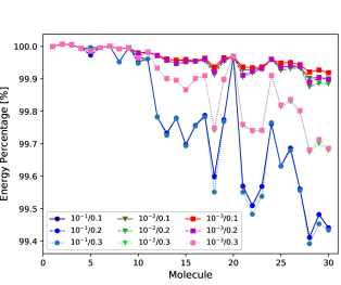
Figure 2: *

(a)

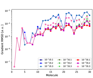
Figure 3: *

(b)

Figure 4: Comparisons of the percentages of correlation energy (a) and the RMSDs (root mean square deviations) of gradient (b) between the MBE(3)-OSV-MP2 ($l_{\textrm{osv}}=10^{-4}$) and canonical RI-MP2 with respect to the 2b and 3b cluster selections ($l_{\textrm{2b}}/l_{\textrm{3b}}$). The basis set def2-tzvp was used for all computations.

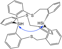
Figure 5: *

BHS

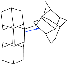
Figure 6: *

DIAD

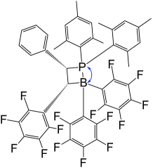
Figure 7: *

FLP

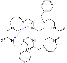
Figure 8: *

YIVNOG

Figure 9: Medium size molecules for assessing MBE(3)-OSV-MP2 geometries for which the canonical RI-MP2 reference structures can be computed.

The MBE(3)-OSV-MP2 structures of several representative medium size molecules containing different connectivities from second and third row elements (BHS, FLP, DIAD and YIVNOG in Figure 9) are compared to RI-MP2 reference geometries. The deviations of selected interatomic distances are given in Table 2. The maximal relative deviations from the RI-MP2 interatomic distance are about 0.4%, 0.3%, 0.09% and 0.4% for BHS, DIAD, FLP and YIVNOG, respectively, with the magnitudes varying between 0.1 and 1.7 pm. The MBE(3)-OSV-MP2 accuracy is similar to that of normal OSV-MP2 using the same $l_{\textrm{osv}}=10^{-4}$. The largest errors take place to BHS Si-Si distance (1.7 pm) of C₁ symmetry and YIVNOG O-N distance (1.3 pm), both between non-bonded atoms residing remotely on the periphery of the cavity. The MBE(3)-OSV-MP2 errors for bonded atoms are however as small as about 0.5 pm for DIAD C-C and 0.1 pm for FLP P-B bond. Overall, the MBE(3)-OSV-MP2 optimized structures are sufficiently accurate compared to RI-MP2 benchmarks, and can be obtained by terminating the MBE(3) expansion on a small amount of important 2b and 3b clusters (Table 2). The improvements of bond lengths for BHS and YIVNOG are very limited by including more 3b clusters using $l_{\text{3b}}=0.1$, for which the numbers of 3b clusters are however considerably increased from 6112 and 8560 to 9886 and 13852, respectively.

Table 2: Comparisons of correlation energy percentages ($|\delta E_{c}|$) and optimized interatomic distance deviations ($|\delta d|$) between MBE(3)-OSV-MP2, normal OSV-MP2 and canonical RI-MP2 using def2-tzvp basis and frozen core approximation. The structure convergence meets three criteria: the energy change ($\leq 10^{-6}$ au), the gradient RMS (root mean square, $\leq 3\times 10^{-4}$ au) and the maximum gradient ($\leq 4.5\times 10^{-4}$ au). RI-MP2 structures were obtained using the ORCA program package⁹⁸ with RIJK integrals.

molecules	BHS (Si-Si)	DIAD (C-C)	FLP (P-B)	YIVNOG (O-N)
$N_{\text{atom}}~{}^{a}$	76	82	88	116
$N_{\text{orb}}~{}^{b}$	1586	1392	2059	2046
$N_{\text{aux}}~{}^{c}$	4009	3426	5078	5034
$N_{2b}~{}^{d}$	5671	4465	12403	10878
$N_{3b}~{}^{e}$	198485	138415	644956	529396
RI-MP2 reference	441.4	168.2	209.6	307.8
OSV-MP2 $l_{\mathrm{osv}}=10^{-4}$
$|\delta E_{c}|$ (%)	99.79	99.64	99.78	99.77
$|\delta d|$ (pm)	1.3	0.4	0.2	1.0
MBE(3)-OSV-MP2 $l_{\mathrm{osv}}=10^{-4},l_{\mathrm{2b}}=10^{-2},l_{\mathrm{3b}}=0.2$
$\tilde{N}_{2b}~{}^{f}$	1772	2003	3213	2670
$\tilde{N}_{3b}~{}^{g}$	6112	7065	10785	8560
$|\delta E_{c}|$ (%)	99.78	99.65	99.72	99.77
$|\delta d|$ (pm)	1.7	0.5	0.2	1.1
MBE(3)-OSV-MP2 $l_{\mathrm{osv}}=10^{-4},l_{\mathrm{2b}}=10^{-2},l_{\mathrm{3b}}=0.1$
$\tilde{N}_{2b}~{}^{f}$	1772	2003	3213	2670
$\tilde{N}_{3b}~{}^{g}$	9886	12107	19069	13852
$|\delta E_{c}|$ (%)	99.80	99.69	99.76	99.80
$|\delta d|$ (pm)	1.4	0.4	0.2	0.8
aNumber of atoms. bNumber of orbital basis functions. cNumber of auxiliary fitting functions. dNumber of full 2b clusters. eNumber of full 3b clusters. fNumber of selected 2b clusters. gNumber of selected 3b clusters.

3.1.2 Molecular dynamics simulation

In our previous work ²⁹, we demonstrated that OSV-MP2 permit accurate molecular dynamics (MD) simulations that would be promising for obtaining long-time trajectories at MP2 level of electron correlation. For protonated water tetramer (Eigen, H₉O${}_{4}^{+}$) and hexamer (Zundel, H₁₃O${}_{6}^{+}$) which have been often used to benchmark MD accuracy, the OSV-MP2 method leads to accurate landscapes of the O-O/O-H radial distribution function (RDF) and vibrational density of states (VDOS) with all major peaks well replicated using a normal OSV selection ($l_{\textrm{osv}}=10^{-4}$) compared to RI-MP2 benchmark. Here we further investigate the reliability of these MD properties derived from MBE(3)-OSV-MP2 gradients using selected 2b and 3b clusters to propagate classical MBE(3)-OSV-MP2/NVE trajectories for 10 ps in numerical time integration at an interval of every 0.5 fs using the i-PI software ⁹⁹. As a result, the MBE(3)-OSV-MP2/6-31+g(d,p) MD simulation leads to energy drifts of 1.3 kJ/mol and 1.1 kJ/mol for the protonated Eigen (H₉O${}^{+}_{4}$) and Zundel (H₁₃O${}^{+}_{6}$) clusters, respectively, which are greater than the corresponding normal OSV-MP2 results (0.0 and 0.1 kJ/mol) without using MBE(3). The energy drift, which measures the energy conservation property of NVE simulation deviated from the linear least-square fit to the trajectory at all time steps, reflects that the error propagation due to the OSV and cluster selections is still within chemical accuracy. The increased energy drift for MBE(3)-OSV-MP2 does not necessarily alter the VDOS (Figure 12) and RDF (Figure 17) spectra beyond statistical variance, and all VDOS and RDF features are retrieved from MBE(3)-OSV-MP2 MD simulations, as compared to those of normal OSV-MP2.

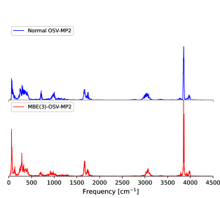
Figure 10: *

(a) Eigen H₉O${}_{4}^{+}$

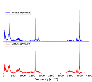
Figure 11: *

(b) Zundel H₁₃O${}_{6}^{+}$

Figure 12: Comparison of VDOS spectra between MBE(3)-OSV-MP2 and normal OSV-MP2 implementations for Eigen (a) and Zundel (b) clusters. VDOS spectra were computed by taking the fast Fourier transform of the velocity auto-correlation function.

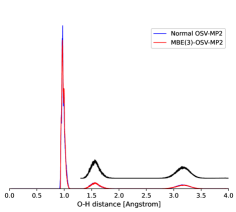
Figure 13: *

(a) O-H H₉O${}_{4}^{+}$

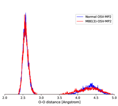
Figure 14: *

(b) O-O H₉O${}_{4}^{+}$

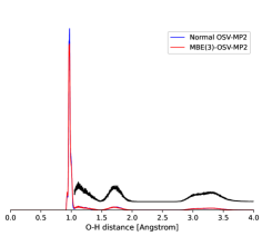
Figure 15: *

(c) O-H H₁₃O${}_{6}^{+}$

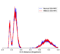
Figure 16: *

(d) O-O H₁₃O${}_{6}^{+}$

Figure 17: RDF Comparison for O-H (left) and O-O (right) distances for Eigen (a, b) and Zundel (c, d) clusters between MBE(3)-OSV-MP2 and normal OSV-MP2 implementations. The weak O-H spectra above 1.0 Å are magnified in black, showing O-H distances associated with hydrogen bonding and non-bonding distribution. RDFs were prepared for full trajectories using VMD program ¹⁰⁰.

3.2 High-order MBE($n$) ($n>3$) Contribution

MBE(3)-OSV-MP2 correlation energies and gradients demonstrated to Baker molecules in Figure 4 disclose the importance of 3b contributions, which increases as molecular size increases. Neglect of 3b clusters apparently results in unacceptable errors of both energy and gradient relative to RI-MP2. Figure 4 also seems to suggest that the higher-order MBE($n$) ($n>3$) contributions beyond the 3-body level of correlation are minor. For dynamical properties of protonated water tetramer and hexamer, the higher-order errors in the MBE(3)-OSV-MP2/NVE simulation are only marginally larger than $1.0$ kJ/mol, close to chemical accuracy, and do not make meaningful changes to the landscapes of O-O/O-H VDOS and RDF. The insignificance of higher-order contributions can avoid a vast number of distinct MBE($n$) ($n>3$) clusters in otherwise catastrophic nonlinear growth with system size that presents undesired challenges in handling efficient cutoffs of them.

To further demonstrate that the actual impact arising from MBE($n$) ($n>3$) clusters on energy and gradient of large molecules is insignificant, we estimate the residual error $\delta\mathbf{R}_{(ij,ij)}$ according to eq 4, using the converged MBE(3)-OSV-MP2 collective pair amplitudes $\mathbf{T}_{(ij,ij)}$ by which $ij$ pairs can correlate with a range of $k$ LMOs among the union of 1b, 2b and 3b clusters, and compute the amplitude correction $\delta\mathbf{T}_{(ij,ij)}$ in one step. This one step posterior correction not only couples all independent cluster amplitudes, but also correlates each pair $ij$ with a range of close $k$ LMOs which is shown small for large molecules using triplet-$\zeta$ basis sets, for instances, up to 13 LMOs are found significant for BHS, DIAD, FLP, YIVNOG and C₆₀@catcher, and up to 10 LMOs for (H₂O)₁₉₀, barely adding timing costs compared to iterative MBE(3) residual. Figure 22 illustrates the high-order MBE($n$) impact to both correlation energies and gradients, using the RI-MP2 structures of BHS, DIAD, FLP and YIVNOG molecules. The high-order contributions appear to be unimportant, as compared to normal OSV-MP2 results, for both OSV selections of $l_{\text{osv}}=10^{-4}$ and $l_{\text{osv}}=10^{-4.5}$. Such corrections from the full range of $k$ LMOs are also computed and presented in Figure S3, which improves both MBE(3) energies and gradients at the 3b level towards normal OSV-MP2 results, with yet a very small magnitude within $0.05\%$ and $10^{-4}$ au, respectively. This implies that the 3b level of cluster truncation is indeed sufficient to achieve the accuracy of energy and gradient, close to that of normal OSV-MP2.

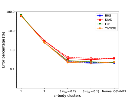
Figure 18: *

(a) $l_{\text{osv}}=10^{-4}$, $l_{\text{2b}}=10^{-2}$

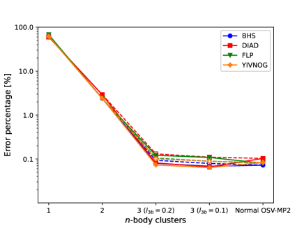
Figure 19: *

(b) $l_{\text{osv}}=10^{-4.5}$, $l_{\text{2b}}=10^{-2}$

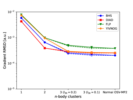
Figure 20: *

(c) $l_{\text{osv}}=10^{-4}$, $l_{\text{2b}}=10^{-2}$

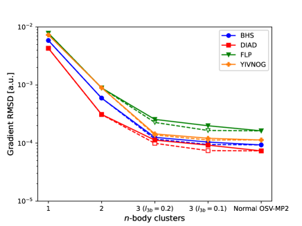
Figure 21: *

(d) $l_{\text{osv}}=10^{-4.5}$, $l_{\text{2b}}=10^{-2}$

Figure 22: Errors in 1b, 2b and 3b clusters to MBE(3)-OSV-MP2 correlation energy (a and b: percentage) and gradient (c and d: RMSD) from those of RI-MP2, for BHS, DIAD, FLP and YIVNOG molecules computed at the def2-tzvp basis set. The normal OSV-MP2 uses the orbital pairs from kept 2b clusters. The high-order one-step corrections to the collective amplitude are shown in dashed lines.

3.3 Scaling and Parallel Performance

In this section, we assess the scaling and parallel efficiency of MBE(3)-OSV-MP2 energy and gradient implementations with increasing system sizes and CPU numbers. Polyglycine chains (Gly)_n comprising up to $n=40$ units were used for the scaling demonstration. As shown in Figure S2, with $l_{\text{2b}}=10^{-2}$ and $l_{\text{3b}}=0.2$, the numbers of selected 2b and 3b clusters exhibit nice linear growths with the (Gly)_n lengths and are reduced by at least an order of magnitude from the full cluster size for (Gly)₄₀. The overall elapsed time of MBE(3)-OSV-MP2 energy and gradient scales according to $N^{1.59}$ and $N^{2.26}$ up to (Gly)₁₄, respectively as shown in Figure 25a, which greatly improves the computing performance of our previous OSV-MP2 implementation with $N^{2.74}$ for energy and $N^{2.96}$ for gradient ²⁹ for similar molecular sizes. The energy and gradient scalings increase to $N^{1.98}$ and $N^{2.60}$ towards larger (Gly)₄₀, respectively, due to significantly larger half-integrals $\mathbf{J}_{i}$ and $\mathbf{Y}_{i}$ intermediates that are stored on shared disk and considerably increasing I/O bottleneck. Nevertheless, although the timing cost does not scale linearly with system size, the present implementation already allows efficient gradient computations of large molecule containing a few hundred atoms, and meanwhile benefits fast MD simulations of smaller molecule. For instances, using normal cutoffs of OSVs ($l_{\mathrm{osv}}=10^{-4}$) and MBE(3) clusters ($l_{\mathrm{2b}}=10^{-2}$, $l_{\mathrm{3b}}=0.2$), each single MBE(3)-OSV-MP2/def2-tzvp energy and gradient computation of C₆₀@catcher complex (148 atoms) takes only 34 and 190 minutes on 24 CPUs, respectively; the MBE(3)-OSV-MP2/6-31g* MD simulation runs on 1–2 ps trajectory length per day for porphycene molecule on 96 CPUs.

To understand the algorithmic complexities pertinent to the current implementation, we further analyze the scaling performance of various dominating steps within a single MBE(3)-OSV-MP2 gradient computation. As presented in Figure 25b, the residual time cost for amplitudes is negligibly small and scales almost linearly with (Gly)_n sizes according to $N^{1.19}$ as a result of the linear growth of 2b and 3b clusters. The time complexity for OSV-specific residual relaxation $\mathbf{R}^{\{\lambda\}}$ is shortened from $N^{6}$ to $N^{2.29}$ owing to massive truncations of OSVs, discarded OSV relaxation vectors and MBE(3) clusters. The time of generating exact OSVs increases rapidly at $N^{4}$ with (Gly)_n length which eventually contributes to a large fraction of overall time expense for large molecule, but can be reduced dramatically to $N^{2.39}$ with negligible time cost by employing approximate ID-OSVs. The 3c2e half-transformation $\left(i\alpha|A\right)$ and the evaluation of resulting OSV-based 4c2e integrals spend only moderate timings with a scaling reduction from original $N^{4}$ to $N^{2.71}$ and from $N^{5}$ to $N^{2.64}$, respectively, by the AO shell pair screening, sparse fitting as well as selection of OSVs and MBE(3) clusters. The most expensive steps for gradient computation appear to be associated with two-electron terms in, such as, the $\mathbf{Y}_{i}$ intermediate ($N^{3.11}$), the Z-vector potential ($N^{2.47}$) and the derivative AO integrals $\left(\alpha\beta|A\right)^{(\lambda)}$ ($N^{2.47}$), all of which add up to about half of the overall gradient time. This indicates that the performance for very large molecules begins to be certainly bounded to these predominant costs. For energy alone, the computation of OSV two-electron integrals $\mathbf{K}_{(ij,ij)}$ for strong 2b clusters dominates the timing cost, while the timing of $\mathbf{K}_{(i,j)}$ for weak 2b clusters is negligible.

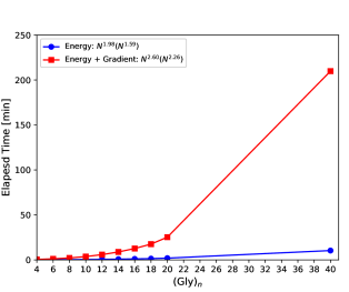
Figure 23: *

(a)

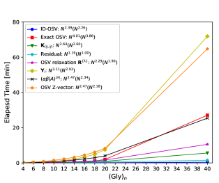
Figure 24: *

(b)

Figure 25: Elapsed time of computing MBE(3)-OSV-MP2 correlation energy and gradient (a) as well as various dominating steps (b) for polyglycine (Gly)_n with def2-tzvp basis set on 24 CPU cores (Intel Xeon Platinum 9242@2.30GHz). The scaling powers are presented in the legend for up to (Gly)₄₀ and (Gly)₁₄ in the parentheses. The 3c2e half-integrals $\mathbf{J}_{i}$ were computed and placed on disk. The computations of LMOs and $\mathbf{J}_{i}$ are not included in MBE(3)-OSV-MP2 energy and overall scaling.

Next, we demonstrate the parallel speedups with respect to the number of CPUs presented in Figure 28 for (Gly)₂₀ and C₆₀@catcher complexes. For (Gly)₂₀ computed on 2–24 CPUs, a satisfactory parallel speedup of MBE(3)-OSV-MP2 gradient computation is achieved, relative to that using 2 CPUs. For larger C₆₀@catcher molecule, three- and four-fold speedups in elapsed time are observed on 72 and 120 CPUs compared to the timing on 24 CPUs, respectively. Overall, a parallel scalability is nearly 100% for a smaller number of CPUs and drops to 80% when a large number of CPUs is employed. Although our implementation is based on passive one-sided communication of supposedly low synchronization latency, it is inevitable that the number of parallel I/O disk accesses grows with increasing number of CPUs, and more importantly, the uneven distribution of parallel tasks becomes an issue that further adds synchronization overheads and reduces the parallel scalability.

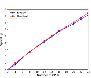
Figure 26: *

(a) (Gly)₂₀

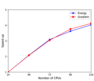
Figure 27: *

(b) C₆₀@catcher

Figure 28: Parallel speedups in elapsed time of MBE(3)-OSV-MP2 energy and gradient computations with an increasing number of CPUs (Intel Xeon Platinum 9242@2.30GHz) for (Gly)₂₀ (a) and 120 CPUs across 10 nodes (Intel Xeon E5-2692 v2@2.20 GHz) for C₆₀@catcher (b).

Finally, we take C₆₀@catcher and (H₂O)₁₉₀ (Figure 31) as examples to demonstrate the performance of parallel MBE(3)-OSV-MP2 gradient computation for large molecules. The timing results for a single gradient computation are given in Table 3. The total elapsed time of the parallel energy and gradient computations is about 190 minutes for C₆₀@catcher/def2-tzvp, 543 minutes for (H₂O)₁₉₀/vdz and 3588 minutes for (H₂O)₁₉₀/vtz on 24 CPUs. The correlation energy computation of MBE(3)-OSV-MP2 alone takes about only 30 minutes for C₆₀@catcher/def2-tzvp, 72 minutes for (H₂O)₁₉₀/vdz and 806 minutes for (H₂O)₁₉₀/vtz. Further timing speedup can be achieved when more CPU resources become available, for instance, there is a four-fold speedup on 120 CPUs for C₆₀@catcher, which makes it now feasible to afford structure optimization for large molecules with a few thousand orbital functions and ten thousand fitting functions in a reasonable time. Again, we find that the bottleneck steps still point to the computation of $\mathbf{Y}_{i}$, the derivative integrals $(\alpha\beta|A)^{(\lambda)}$ and the OSV Z-vector solution, which take the time fractions of 23.7%, 16.2% and 38.0% for C₆₀@catcher, 18.8%, 27.2% and 34.4% for (H₂O)₁₉₀/vdz, as well as 21.8%, 21.9% and 22.2% for (H₂O)₁₉₀/vtz. Solving OSV Z-vector equation takes up the largest portion of the MBE(3)-OSV-MP2 gradient time for both systems, as the evaluation of $\sum_{kl}{\Lambda}_{kl}\mathcal{B}_{kl,ai}$ belonging to the Z-vector source term $W_{ia}$ of eq 24 is rather inefficient in our current implementation. It is noticed that the exact OSV generation costs 403 minutes that is about half of the energy computational time for (H₂O)₁₉₀ using triplet-$\zeta$ basis set, but this is dramatically reduced to only 22 minutes when approximate ID-OSV (section 2.2.3) is generated.

Figure 29: *

C₆₀@catcher

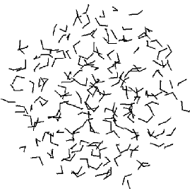
Figure 30: *

(H₂O)₁₉₀

Figure 31: Chemical formula of large molecules for MBE(3)-OSV-MP2 application. The coordinate of C₆₀@catcher is from ref.¹⁰¹ and that of (H₂O)₁₉₀ is from ref.¹⁰².

Table 3: Comparisons of elapsed time (minutes) and timing fraction (%) in various MBE(3)-OSV-MP2 energy and gradient steps for single-point computations of C₆₀@catcher and (H₂O)₁₉₀ on 24 CPUs (Intel Xeon Platinum 9242@2.30GHz).

Molecular sizes	C60@catcher		(H2O)190
basis set	def2-tzvp		cc-pvdz		cc-pvtz
atoms	148		570		570
orbital basis	3888		4560		11020
MP2 fitting basis	9540		15960		26790
Main steps	Time	Fraction	Time	Fraction	Time	Fraction
$(i\alpha|A)$	9.4	5.0	39.1	7.2	264.8	7.4
exact OSV	6.6	3.4	17.6	3.2	402.9	11.2
(ID-OSV)	(1.9)		(1.9)		(22.5)
OSV $\mathbf{S}/\mathbf{F}$	0.3	0.2	0.3	0.1	2.8	0.1
OSV $\mathbf{K}$ matrix	6.2	3.3	8.1	1.5	128.7	3.6
residual iteration	6.0	3.2	6.1	1.1	6.4	0.2
residual relaxation $\mathbf{R}^{\{\lambda\}}$	13.5	7.1	34.8	6.4	418.0	11.7
$\mathbf{Y}_{i}$ evaluation	45.1	23.7	102.4	18.8	780.6	21.8
$(\alpha\beta|A)^{(\lambda)}$	30.7	16.2	147.8	27.2	785.8	21.9
OSV Z-vector	72.2	38.0	187.0	34.4	797.6	22.2
total$~{}^{a}$	189.9	100	543.3	100	3587.7	100
aThe total elapsed time is based on the exact OSV generation.

4 ILLUSTRATIVE APPLICATIONS

We showcase two brief applications of MBE(3)-OSV-MP2 gradient implementation to illustrate: (i) the variation of mechanical bond length for tuning catalytic activity of Cu(I) complex supported by interlocked catenane ligands¹⁰³ (Figure 32), and (ii) the N-H vibrational signature associated with $cis$/$trans$ tautomerization due to double hydrogen transfer in porphycene molecule ¹⁰⁴ from the MP2-level electron correlation and classical protons. Both systems demand tremendous tasks in computing analytical energy gradients for structure optimization and MD evolution, which are rather expensive using conventional MP2 method.

4.1 Cu(I)-Catenane Interlocking Coordination Structure

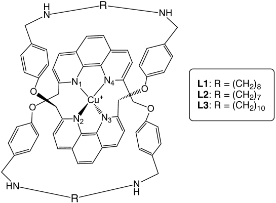
Figure 32: Chemical formula of Cu(I)-catenane complex interlocking L1, L2 and L3 ligands, respectively.

The tetradentate Cu(I) complex mechanically interlocking catenane ligands has been recently demonstrated to selectively catalyze C(sp³)–O dehydrogenation between phenol and bromodicarbonyl¹⁰³. It was found that different catenane topologies and peripheral lengths effectively managed Cu(I)-catenane mechanical bonds by adjusting Cu(I) coordination environment, leading to varying catalytic activity for a broad scope of substrates. The dehydrogenative coupling of phenol and diethyl bromomalonate reveals experimentally that the Cu(L1) and Cu(L3) complexes in relatively loose mechanical bonds with long L1 (R=(CH₂)₈) and L3 (R=(CH₂)₁₀) ligands have a high catalytic activity in nearly 77–80% product yield, while Cu(L2) complex in tight bond with short L2 (R=(CH₂)₇) considerably compromises the product generation at a yield of only 52%.

Table 4: The distances of N-Cu bonds (pm) and the dihedral angles (°) between the N₁-Cu-N₂ and N₃-Cu-N₄ planes for [Cu(L1)]PF₆, [Cu(L2)]PF₆ and [Cu(L3)]PF₆ optimized by MBE(3)-OSV-MP2/def2-tzvp (all electrons) and B3LYP-D3BJ/Lanl2dz/6-31g(d,p). The DFT values were obtained using ORCA software package⁹⁸. $V_{\text{coor}}$ is the volume (pm³) of the coordination cavity which is measured as the Cu-centred polyhedral volume enclosed with four nitrogen vertices.

Method		[Cu(L1)]PF6	[Cu(L2)]PF6	[Cu(L3)]PF6
MBE(3)-OSV-MP2	N1-Cu	202.22	200.22	201.75
	N2-Cu	197.53	197.44	198.26
	N3-Cu	202.30	200.51	201.39
	N4-Cu	197.47	197.12	198.23
	dihedral angle	103.96	104.76	105.23
	$V_{\text{coor}}$	3377975.78	3346818.43	3366231.91
	$\Delta V_{\text{coor}}$	0.00	-31157.35	-11743.87
B3LYP-D3BJ	N1-Cu	205.48	204.50	205.52
	N2-Cu	204.99	208.76	208.21
	N3-Cu	205.48	204.01	205.58
	N4-Cu	205.00	209.68	207.53
	dihedral angle	107.77	105.80	107.86
	$V_{\text{coor}}$	3595533.80	3655158.99	3626158.36
	$\Delta V_{\text{coor}}$	0.00	59625.19	30624.56

The structures of [Cu(L1)]PF₆, [Cu(L2)]PF₆ and [Cu(L3)]PF₆ were optimized at the MBE(3)-OSV-MP2/def2-tzvp level of theory with all electrons correlated. As shown in Table 4, the small change in the number of methylene groups does not make a large impact on the Cu-N distances, nor on the dihedral angles, causing less than 2 pm deviations in Cu-N lengths and 2 degrees in dihedral angles, which can be however consistently distinguished by the MBE(3)-OSV-MP2 method. As shown in Table 4, the polyhedral volume of [Cu(L1)]PF₆ with medium size ligand is larger than those of both [Cu(L3)]PF₆ with the longest ligand by 0.5% and [Cu(L2)]PF₆ with the shortest ligand by 0.9%. The $V_{\text{coor}}$ ordering $\text{[Cu(L1)]P}_{6}>\text{[Cu(L3)]P}_{6}>\text{[Cu(L2)]P}_{6}$ for three catenane ligands agrees with the ranking of their catalytic efficacy by experiments. This indicates that the coordination space accommodating the Cu ion can be adjusted by tuning the ligand length, which creates an open and responsive coordination environment for substrates. However, the Cu coordination volume does not scale proportionally with the length of the catenane ligand due to intricacies of Cu-catenane interlocking interaction and ligand topology. In passing, the structures from MBE(3)-OSV-MP2 are also compared with DFT/B3LYP-D3BJ results. While the MBE(3)-OSV-MP2 predicts a reduction of Cu coordination volume from $\text{[Cu(L1)]P}_{6}$, the B3LYP-D3BJ results are opposite and give a volume expansion with a different ordering $\text{[Cu(L2)]P}_{6}>\text{[Cu(L3)]P}_{6}>\text{[Cu(L1)]P}_{6}$ from that of MBE(3)-OSV-MP2. Our results suggest that these subtle structure changes are indeed susceptible to different correlated energy and gradient models which are critically essential.

4.2 Porphycene Tautomerization from MD Simulation

Porphycene (Pc, C₂₀H₁₄N₄) is a complex prototypical molecule in which a fast double hydrogen transfer (HT) is believed to occur at room temperature along the strong intramolecular hydrogen bonds in the molecular cavity formed by four nitrogens^{105, 104}. This HT-based tautomerization reaction proceeds via an internal $\mathrm{N}-\mathrm{H}\cdots\mathrm{N}$ pathway resulting in different tautomeric isomers: cis-Pc tautomer where two hydrogens are bonded to nitrogens on the same side and trans-Pc tautomer with two hydrogens connected to nitrogens on the other side. However, the standard harmonic frequency calculation assigns only a strong single peak around 2900 cm^-1 to the N-H stretching vibration, while experimental infrared (IR) spectrum shows a significantly broadened and weakened N-H stretching band over 2000–3000 cm^-1. It has been revealed that such a discrepancy results from the lack of vibrational anharmonicity and intermode couplings, since each harmonic N-H mode leads to short N-H vibration that prevents its elongation towards HT and the two independent N-H vibrations uncorrelate double HT pathways. The anharmonic and coupling impacts on the N-H vibrational bands have been investigated from ab-initio MD simulation with density functional theory (DFT) in literature. The N-H vibrational bands from thermostated classical-nuclei MD sampling multiple NVE/DFT trajectories are considerably softened due to the success of recovering the anharmonicity and coupling with low-energy modes, located around 2700–2900 cm^-1 for BLYP/PW¹⁰⁵, 2500 cm^-1 for PBE and 2750–3000 cm^-1 for B3LYP-vdW functional¹⁰⁴. However, the broad N-H signature extending in the lower frequency range is still missing from DFT/MD simulation, and was recently suggested to ascribe to protonic quantum effects based on ring-polymer MD results. Here, we present an alternative interpretation from 10 ps classical-nuclei ab-initio MD/NVE simulation using MBE(3)-OSV-MP2 correlated model, which yields VDOS spectrum that retrieves both broadened low- and high-energy N-H stretching peaks centered at 2600 cm^-1 and 3000 cm^-1 (Figure 33b), respectively, by propagating classical protons.

The MBE(3)-OSV-MP2/MD parallel simulation was carried out on 96 CPUs using an initial porphycene structure from MBE(3)-OSV-MP2/6-31g* optimization. On the average, about 32 seconds (9 seconds for RHF and 23 seconds for MBE(3)-OSV-MP2 energy and gradient evaluations) were spent in each MD step, and the entire 20000 MD steps were completed in less than 8 days. The RDF for N-N distances (Figure 33a) shows that there are two broad peaks between 2.5 and 3.0 Angstrom in which the first peak resembles the signature of the nitrogen pairs involved in proton transfers causing the respective $trans$-Pc and $cis$-Pc tautomerization. As shown in Figure 33a, the peak position is assigned to the N-N pair of $trans$-Pc, while the lower peak shoulder is given to the shorter N-N pair of $cis$-Pc, suggesting more $trans$-Pc. The VDOS spectrum also features the weak $cis$-Pc band centered at 2600 cm^-1 and relatively stronger $trans$-Pc band centered at 3000 cm^-1, which also indicates more $trans$-Pc than $cis$-Pc. In contrast, the literature ring-polymer DFT/MD results however concluded a larger proportion of $cis$-Pc tautomer and thus stronger hydrogen bonds, leading to more hydrogen transfer due to the inclusion of quantal protons. More detailed studies combining both MP2-level correlated electrons and quantal protons are therefore desired.

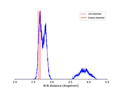
(a)

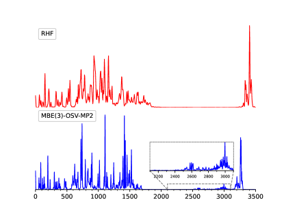
(b)

Figure 33: The MBE(3)-OSV-MP2/6-31g*/MD simulation from a single trajectory for porphycene: the N-N RDF (a) and VDOS (b). The red vertical lines label the distances of equilibrium $trans$-Pc (solid) and $cis$-Pc (dashed). The 10 ps trajectory was generated at a time step of 0.5 fs from the thermostated NVT simulation at the average temperature of 291.9 K (the temperature drift was 1.5 K), followed by another 10 ps NVE run leading to the computed RDF and VDOS results. The MBE(3)-OSV-MP2/MD simulation was carried out on 96 CPUs (Intel Xeon Platinum 9242@2.30GHz).

5 CONCLUSIONS

We have developed a low-order scaling and parallel algorithm for MBE(3)-OSV-MP2 analytical gradient computation of large molecules using the third-order many-body expansion of OSV-MP2 wavefunction and density matrices. By construction, each 1b cluster is orbital-specific to an LMO and computed in the corresponding basis of OSVs, leading to the linearly increasing number of 1b clusters with molecular sizes; the local 2b and 3b clusters are respectively specific to orbital pair and triple correlations and screened to achieve the effective linear growths. Higher-order MBE($n$) ($n>3$) clusters are shown insignificant to both correlation energies and analytical gradients, and can be entirely neglected. By further introducing correlation approximations to long-range 2b clusters and by exploiting the sparsity in density fitting integrals and OSV relaxation vectors, the computational costs are mitigated to the low-order scaling in the linear and quadratic regimes for correlation energy and gradient, respectively. Moreover, by managing the global and local data arrays of selected MBE(3)-OSV-MP2 intermediates in the hybrid RMA and SHM parallelism through passive one-sided communication across multiple nodes, the highly parallelized algorithm conveys an implementation that enables fast and scalable MBE(3)-OSV-MP2 computations of energy and analytical gradient using a large number of CPUs. The computations of $\mathbf{Y}_{i}$ intermediate and Z-vector equation remain the main components to the overall runtime cost to obtain accurate analytical gradients of large molecules of a few hundred atoms. Existing techniques can be envisaged to improve the scalability of these steps. For instances, multipole-based long-range integrals accounting for the asymptotic behaviour of $1/R$ can be utilized to expeditiously estimate two-electron potential in Z-vector equation. Moreover, fast evaluation of two-center or multi-center molecular integrals and their derivatives are recently available  ^{106, 107}. The sparse fittings have not yet been implemented for accelerating evaluation of the product $\mathbf{Y}_{i}^{\dagger}\mathbf{J}_{p}$.

The correlation energies of Baker testing molecules based on the normal selection of MBE(3) clusters are recovered by $>99.85\%$ and the gradient RMSDs are $<3\times 10^{-4}$ au from those of canonical RI-MP2, which are mostly comparable to the original OSV-MP2 results using the same OSV set. The optimized structures have been benchmarked for medium size molecules containing second and third row elements, using up to two thousand basis functions and five thousand fitting functions. The selections of OSVs ($l_{\text{osv}}=10^{-4}$), 2b clusters ($l_{\text{2b}}=10^{-2}$) and 3b clusters ($l_{\text{3b}}=0.1$) yield small MBE(3)-OSV-MP2 errors of 0.1–0.5 pm for short bonded interatomic distances and 1.1–1.5 pm for long non-bonded distances, using only a small fraction of 2b and 3b clusters. The NVE MD simulations of protonated water tetramer and hexamer driven by MBE(3)-OSV-MP2 gradients have been performed, and the resulting RDF and VDOS spectra are in excellent agreement to the normal OSV-MP2 benchmarks. The efficiencies and capabilities of the MBE(3)-OSV-MP2 gradient implementation were further demonstrated in parallel computations of C₆₀@catcher (148 atoms) and (H₂O)₁₉₀ (570 atoms) molecules on 24 CPUs, with the total runtime of about 2.7 and 46 hours in a single gradient step with def2-tzvp and cc-pvtz basis sets, respectively. Finally, in two brief applications, we show that the MBE(3)-OSV-MP2 algorithm permits the differentiation of the subtle structure changes in interlocked Cu-catenane supramolecule by varying ligand length, and also 10 picoseconds long MD simulation of porphycene ($\sim 40$ atoms) that reveals N-H stretching signature associated with inter-convertible tautomers.

The authors acknowledge financial supports from the Hong Kong Research Grant Council (Grant No. ECS27307517 and GRF17309020). We are grateful to the Computational Initiative provided by the Faculty of Science at the University of Hong Kong and Tianhe-2 computing service at the National Supercomputer Center in Guangzhou of China for their technical supports and allocation of CPU hours. J.Y. acknowledges the research program of AIR@InnoHK cluster from the Innovation and Technology Commission of Hong Kong SAR of China. Q.L. thanks Ruiyi Zhou for discussions.

The file Supporting supporting.pdf contains further results of the computations and is available free of charge.

Appendix

Gradient implementation

Algorithm 1 Pseudocode and parallelism for MBE(3)-OSV-MP2 analytical gradients.

***MBE(3)-OSV-MP2 energy***

Parallel tasks on AO shell pairs $(\alpha\beta)$ for $(\alpha\beta|A)$:

 sparse fitting $\mathbf{J}_{i}$ and $\mathbf{T}_{kk}$, placed on shared disk

Parallel tasks on occupied LMOs:

 generation of exact OSVs or ID-OSVs

Parallel tasks on $ij$ pairs in RMA:

 evaluate OSV overlap $\mathbf{S}_{(i,j)}$ and $\mathbf{F}_{(i,j)}$;

 2b and 3b clustering and sorting;

 evaluate $\mathbf{K}_{(ij,ij)}$ and $\mathbf{K}_{(i,j)}$.

Parallel tasks on 1b/2b/3b clusters:

 solve MBE(3)-OSV-MP2 residual equations;

 collect $\mathbf{T}_{(ij,ij)}$ and $\mathbf{R}_{(ij,ij)}$ in RMA.

***MBE(3)-OSV-MP2 gradient***

Parallel tasks on 1b/2b/3b clusters:

 $\mathbf{D}^{\text{1b}},~{}\mathbf{D}^{\text{2b}}~{}\text{and}~{}\mathbf{D}^{\text{3b}}$, $\mathbf{N}_{ij}^{\text{1b}},~{}\mathbf{N}_{ij}^{\text{2b}}~{}\text{and}~{}\mathbf{N}_{ij}^{\text{3b}}$;

  accumulate $\mathbf{D}$ in SHM assigned to root process;

  one-sided accumulation for $\mathbf{N}_{ij}$ in RMA.

Parallel tasks on LMO $i$ batches:

 local loop on $j$ for each task $i$:

  $\mathbf{Y}_{i}\leftarrow\mathbf{Y}_{i}+\mathbf{J}_{j}(\mathbf{Q}_{i}\mathbf{Q}_{j})\mathbf{\overline{T}}_{ij,ij}(\mathbf{Q}_{i}\mathbf{Q}_{j})^{\dagger}$;

  $\mathbf{N}_{i}\leftarrow\mathbf{N}_{i}+\mathbf{N}_{ij}+\overline{\mathbf{T}}_{(ij,ij)}\mathbf{K^{\prime}}_{(ij,ij)}$.

 $\mathbf{X}_{i}=[\mathbf{Q}_{i}(\mathbf{N}_{i}\Delta\mathbf{G}_{ii})\mathbf{Q}^{\prime\dagger}_{i}]/(f_{aa}+f_{bb}-2f_{ii})$;

 $\mathbf{Y}_{i}\leftarrow\mathbf{Y}_{i}+\mathbf{J}_{i}(\mathbf{X}_{i}+\mathbf{X}^{\dagger}_{i})$, stored on shared disk.

Parallel tasks on batches $A$ for $(\alpha\beta|A)$ and $(\alpha\beta|A)^{(\lambda)}$:

 $\mathbf{y}(A)+=\mathbf{y}(A)$; $\mathbf{y^{\prime}}(A)+=\mathbf{y^{\prime}}(A)$; collect $\sum_{i}\braket{\mathbf{P}_{v}\mathbf{Y}_{i}^{\dagger}\mathbf{J}_{i}^{(\lambda)}}$.

Evaluate $\sum_{i}\mathbf{P}_{v}\mathbf{Y}_{i}^{\dagger}\mathbf{J}_{i}$ and $\braket{\mathbf{P}_{v}\mathbf{Y}_{i}^{\dagger}\mathbf{J}_{p}}$ on root process.

***OSV Z-vector***

Parallel on AO shell pairs $(\alpha\beta)$ for RHF $(\alpha\beta|A)$:

 $(i\beta|A)=\sum_{\alpha\beta}(\alpha\beta|A)C_{\alpha i}$; $(\tilde{i}\beta|A)=\sum_{\alpha\beta}(\alpha\beta|A)Z_{\alpha i}$.

Parallel tasks on LMO $i$ batches:

 sparse fittings for $J_{i,A^{\prime}\alpha}$, $J_{i,A^{\prime}j}$ and $J^{\prime\prime}_{i,A^{\prime\prime}j}$;

 update $\Gamma_{A^{\prime}}=\sum_{\alpha i}J_{i,A^{\prime}\alpha}Z_{\alpha i}$;

 $K_{\alpha i}\leftarrow K_{\alpha i}+\sum_{jA^{\prime}}J_{j,A^{\prime}\alpha}J_{i,A^{\prime}j}+\sum_{jA^{\prime\prime}}(\tilde{i}\alpha|A^{\prime\prime})J^{\prime\prime}_{i,A^{\prime\prime}j}$;

 $J_{\alpha i}\leftarrow J_{\alpha i}+\sum_{A^{\prime}}J_{i,A^{\prime}\alpha}\Gamma_{A^{\prime}}$;

 $U_{ai}+=4J_{\alpha i}-K_{\alpha i}$.

Solve OSV Z-vector equation.

References

- Pulay 1983 Pulay, P. Localizability of dynamic electron correlation. Chem. Phys. Lett. 1983, 100, 151–154
- Kohn 1996 Kohn, W. Density functional and density matrix method scaling linearly with the number of atoms. Phys. Rev. Lett. 1996, 76, 3168–3171
- Maslen and Head-Gordon 1998 Maslen, P.; Head-Gordon, M. Non-iterative local second order Møller–Plesset theory. Chem. Phys. Lett. 1998, 283, 102–108
- Ayala and Scuseria 1999 Ayala, P. Y.; Scuseria, G. E. Linear scaling second-order Møller–Plesset theory in the atomic orbital basis for large molecular systems. J. Chem. Phys. 1999, 110, 3660–3671
- Lee et al. 2000 Lee, M. S.; Maslen, P. E.; Head-Gordon, M. Closely approximating second-order Møller–Plesset perturbation theory with a local triatomics in molecules model. J. Chem. Phys. 2000, 112, 3592–3601
- Doser et al. 2009 Doser, B.; Lambrecht, D. S.; Kussmann, J.; Ochsenfeld, C. Linear-scaling atomic orbital-based second-order Møller–Plesset perturbation theory by rigorous integral screening criteria. J. Chem. Phys. 2009, 130, 064107
- Yang et al. 2011 Yang, J.; Kurashige, Y.; Manby, F. R.; Chan, G. K. Tensor factorizations of local second-order Møller–Plesset theory. J. Chem. Phys. 2011, 134, 044123
- Kurashige et al. 2012 Kurashige, Y.; Yang, J.; Chan, G. K.-L.; Manby, F. R. Optimization of orbital-specific virtuals in local Møller–Plesset perturbation theory. J. Chem. Phys. 2012, 136, 124106
- Werner et al. 2015 Werner, H.-J.; Knizia, G.; C., K.; Schwilk, M.; Dornbach, M. Scalable electron correlation methods. I. PNO–LMP2 with linear scaling in the molecular size and near–inverse–linear scaling in the number of processors. J. Chem. Theory Comput. 2015, 11, 484––507
- Hampel and Werner 1996 Hampel, C.; Werner, H.-J. Local treatment of electron correlation in coupled cluster theory. J. Chem. Phys. 1996, 104, 6286–6297
- Schütz and Werner 2000 Schütz, M.; Werner, H.-J. Local perturbative triples correction (T) with linear cost scaling. Chem. Phys. Lett. 2000, 318, 370–378
- Schütz and Werner 2001 Schütz, M.; Werner, H.-J. Low-order scaling local electron correlation methods. IV. Linear scaling local coupled-cluster (LCCSD). J. Chem. Phys. 2001, 114, 661–681
- Schütz 2002 Schütz, M. Low-order scaling local electron correlation methods. V. Connected triples beyond (T): Linear scaling local CCSDT-1b. J. Chem. Phys. 2002, 116, 8772–8785
- Schütz 2002 Schütz, M. A new, fast, semi-direct implementation of linear scaling local coupled cluster theory. Phys. Chem. Chem. Phys. 2002, 4, 3941–3947
- Subotnik and Head-Gordon 2005 Subotnik, J. E.; Head-Gordon, M. A local correlation model that yields intrinsically smooth potential-energy surfaces. J. Chem. Phys. 2005, 123, 064108
- Auer and Nooijen 2006 Auer, A. A.; Nooijen, M. Dynamically screened local correlation method using enveloping localized orbitals. J. Chem. Phys. 2006, 125, 024104
- Subotnik et al. 2008 Subotnik, J. E.; Sodt, A.; Head-Gordon, M. The limits of local correlation theory: Electronic delocalization and chemically smooth potential energy surfaces. J. Chem. Phys. 2008, 128, 034103
- Neese et al. 2009 Neese, F.; Hansen, A.; Liakos, D. G. Efficient and accurate approximations to the local coupled cluster singles doubles method using a truncated pair natural orbital basis. J. Chem. Phys. 2009, 131, 064103
- Werner and Schütz 2011 Werner, H.-J.; Schütz, M. An efficient local coupled cluster method for accurate thermochemistry of large systems. J. Chem. Phys. 2011, 135, 144116
- Yang et al. 2012 Yang, J.; Chan, G. K.-L.; Manby, F. R.; Schütz, M.; Werner, H.-J. The orbital-specific-virtual local coupled cluster singles and doubles method. J. Chem. Phys. 2012, 136, 144105
- Schütz et al. 2013 Schütz, M.; Yang, J.; Chan, G. K.-L.; Manby, F. R.; Werner, H.-J. The orbital-specific virtual local triples correction: OSV–L(T). J. Chem. Phys. 2013, 138, 054109
- Riplinger and Neese 2013 Riplinger, C.; Neese, F. An efficient and near linear scaling pair natural orbital based local coupled cluster method. J. Chem. Phys. 2013, 138, 034106
- Riplinger et al. 2013 Riplinger, C.; Sandhoefer, B.; Hansen, A.; Neese, F. Natural triple excitations in local coupled cluster calculations with pair natural orbitals. J. Chem. Phys. 2013, 139, 134101
- Meyer 1971 Meyer, W. Ionization energies of water from PNO-CI calculations. Int. J. Quantum Chem. 1971, 5, 341–348
- Ahlrichs et al. 1975 Ahlrichs, R.; Lischka, H.; Staemmler, V.; Kutzelnigg, W. PNO–CI (pair natural orbital configuration interaction) and CEPA–PNO (coupled electron pair approximation with pair natural orbitals) calculations of molecular systems. I. Outline of the method for closed-shell states. J. Chem. Phys. 1975, 62, 1225–1234
- Pinski and Neese 2018 Pinski, P.; Neese, F. Communication: Exact analytical derivatives for the domain-based local pair natural orbital MP2 method (DLPNO-MP2). J. Chem. Phys. 2018, 148, 031101
- Pinski and Neese 2019 Pinski, P.; Neese, F. Analytical gradient for the domain-based local pair natural orbital second order Møller–Plesset perturbation theory method (DLPNO-MP2). J. Chem. Phys. 2019, 150, 164102
- Stoychev et al. 2021 Stoychev, G. L.; Auer, A. A.; Gauss, J.; Neese, F. DLPNO-MP2 second derivatives for the computation of polarizabilities and NMR shieldings. J. Chem. Phys. 2021, 154, 164110
- Zhou et al. 2019 Zhou, R.; Liang, Q.; Yang, J. Complete osv-mp2 analytical gradient theory for molecular structure and dynamics simulations. J. Chem. Theory Comput. 2019, 16, 196–210
- Förner et al. 1985 Förner, W.; Ladik, J.; Otto, P.; Cížek, J. Coupled-cluster studies. II. The role of localization in correlation calculations on extended systems. Chem. Phys. 1985, 97, 251–262
- Li and Li 2004 Li, W.; Li, S. Divide-and-conquer local correlation approach to the correlation energy of large molecules. J. Chem. Phys. 2004, 121, 6649–6657
- Kobayashi et al. 2006 Kobayashi, M.; Akama, T.; Nakai, H. Second-order Møller–Plesset perturbation energy obtained from divide-and-conquer Hartree-Fock density matrix. J. Chem. Phys. 2006, 125, 204106
- Stoll 1992 Stoll, H. Correlation energy of diamond. Phys. Rev. B 1992, 46, 6700
- Stoll 1992 Stoll, H. On the correlation energy of graphite. J. Chem. Phys. 1992, 97, 8449–8454
- Doll et al. 1995 Doll, K.; Dolg, M.; Fulde, P.; Stoll, H. Correlation effects in ionic crystals: The cohesive energy of MgO. Phys. Rev. B 1995, 52, 4842
- Kalvoda et al. 1998 Kalvoda, S.; Dolg, M.; Flad, H.-J.; Fulde, P.; Stoll, H. Ab initio approach to cohesive properties of GdN. Phys. Rev. B 1998, 57, 2127
- Friedrich et al. 2007 Friedrich, J.; Hanrath, M.; Dolg, M. Fully automated implementation of the incremental scheme: Application to CCSD energies for hydrocarbons and transition metal compounds. J. Chem. Phys. 2007, 126, 154110
- Friedrich and Dolg 2008 Friedrich, J.; Dolg, M. Implementation and performance of a domain-specific basis set incremental approach for correlation energies: Applications to hydrocarbons and a glycine oligomer. J. Chem. Phys. 2008, 129, 244105
- Friedrich and Dolg 2009 Friedrich, J.; Dolg, M. Fully automated incremental evaluation of MP2 and CCSD (T) energies: Application to water clusters. J. Chem. Theory Comput. 2009, 5, 287–294
- Kállay 2015 Kállay, M. Linear-scaling implementation of the direct random-phase approximation. J. Chem. Phys. 2015, 142, 204105
- Nagy et al. 2016 Nagy, P. R.; Samu, G.; Kállay, M. An integral-direct linear-scaling second-order Møller–Plesset approach. J. Chem. Theory Comput. 2016, 12, 4897–4914
- Flocke and Bartlett 2004 Flocke, N.; Bartlett, R. J. A natural linear scaling coupled-cluster method. J. Chem. Phys. 2004, 121, 10935–10944
- Hughes et al. 2008 Hughes, T. F.; Flocke, N.; Bartlett, R. J. Natural linear-scaled coupled-cluster theory with local transferable triple excitations: Applications to peptides. J. Phys. Chem. A 2008, 112, 5994–6003
- Li et al. 2002 Li, S.; Ma, J.; Jiang, Y. Linear scaling local correlation approach for solving the coupled cluster equations of large systems. J. Comput. Chem. 2002, 23, 237–244
- Li et al. 2006 Li, S.; Shen, J.; Li, W.; Jiang, Y. An efficient implementation of the “cluster-in-molecule” approach for local electron correlation calculations. J. Chem. Phys. 2006, 125, 074109
- Li et al. 2009 Li, W.; Piecuch, P.; Gour, J. R.; Li, S. Local correlation calculations using standard and renormalized coupled-cluster approaches. J. Chem. Phys. 2009, 131, 114109
- Rolik and Kállay 2011 Rolik, Z.; Kállay, M. A general-order local coupled-cluster method based on the cluster-in-molecule approach. J. Chem. Phys. 2011, 135, 104111
- Rolik et al. 2013 Rolik, Z.; Szegedy, L.; Ladjánszki, I.; Ladóczki, B.; Kállay, M. An efficient linear-scaling CCSD (T) method based on local natural orbitals. J. Chem. Phys. 2013, 139, 094105
- Kitaura et al. 1999 Kitaura, K.; Ikeo, E.; Asada, T.; Nakano, T.; Uebayasi, M. Fragment molecular orbital method: an approximate computational method for large molecules. Chem. Phys. Lett. 1999, 313, 701–706
- Nagata et al. 2011 Nagata, T.; Fedorov, D. G.; Kitaura, K. Mathematical formulation of the fragment molecular orbital method. Linear-Scaling Techniques in Computational Chemistry and Physics: Methods and Applications 2011, 17–64
- Fedorov et al. 2012 Fedorov, D. G.; Nagata, T.; Kitaura, K. Exploring chemistry with the fragment molecular orbital method. Phys. Chem. Chem. Phys. 2012, 14, 7562–7577
- Gordon et al. 2012 Gordon, M. S.; Fedorov, D. G.; Pruitt, S. R.; Slipchenko, L. V. Fragmentation methods: A route to accurate calculations on large systems. Chem. Rev. 2012, 112, 632–672
- Hirata et al. 2005 Hirata, S.; Valiev, M.; Dupuis, M.; Xantheas, S. S.; Sugiki, S.; Sekino, H. Fast electron correlation methods for molecular clusters in the ground and excited states. Mol. Phys. 2005, 103, 2255–2265
- Dahlke and Truhlar 2007 Dahlke, E. E.; Truhlar, D. G. Electrostatically embedded many-body expansion for large systems, with applications to water clusters. J. Chem. Theory Comput. 2007, 3, 46–53
- Hirata 2008 Hirata, S. Fast electron-correlation methods for molecular crystals: An application to the , 1, and 2 modifications of solid formic acid. J. Chem. Phys. 2008, 129, 204104
- Fujita et al. 2011 Fujita, T.; Nakano, T.; Tanaka, S. Fragment molecular orbital calculations under periodic boundary condition. Chem. Phys. Lett. 2011, 506, 112–116
- Bygrave et al. 2012 Bygrave, P.; Allan, N.; Manby, F. The embedded many-body expansion for energetics of molecular crystals. J. Chem. Phys. 2012, 137, 164102
- Wen and Beran 2011 Wen, S.; Beran, G. J. Accurate molecular crystal lattice energies from a fragment QM/MM approach with on-the-fly ab initio force field parametrization. J. Chem. Theory Comput. 2011, 7, 3733–3742
- Zaleśny et al. 2011 Zaleśny, R.; Papadopoulos, M. G.; Mezey, P. G.; Leszczynski, J. Linear-Scaling Techniques in Computational Chemistry and Physics: Methods and Applications; Springer Science & Business Media, 2011; Vol. 13
- Gordon 2017 Gordon, M. S. Fragmentation: Toward Accurate Calculations on Complex Molecular Systems; John Wiley & Sons, 2017
- Liu and Herbert 2019 Liu, K.-Y.; Herbert, J. M. Energy-screened many-body expansion: A practical yet accurate fragmentation method for quantum chemistry. J. Chem. Theory Comput. 2019, 16, 475–487
- Herbert 2019 Herbert, J. M. Fantasy versus reality in fragment-based quantum chemistry. J. Chem. Phys. 2019, 151, 170901
- Mochizuki et al. 2008 Mochizuki, Y.; Yamashita, K.; Murase, T.; Nakano, T.; Fukuzawa, K.; Takematsu, K.; Watanabe, H.; Tanaka, S. Large scale FMO-MP2 calculations on a massively parallel-vector computer. Chem. Phys. Lett. 2008, 457, 396–403
- Kjærgaard et al. 2017 Kjærgaard, T.; Baudin, P.; Bykov, D.; Eriksen, J. J.; Ettenhuber, P.; Kristensen, K.; Larkin, J.; Liakh, D.; Pawlowski, F.; Vose, A.; Wang, Y.; Poul, J. Massively parallel and linear-scaling algorithm for second-order Møller–Plesset perturbation theory applied to the study of supramolecular wires. Comput. Phys. Commun. 2017, 212, 152–160
- Riplinger et al. 2016 Riplinger, C.; Pinski, P.; Becker, U.; Valeev, E. F.; Neese, F. Sparse maps—A systematic infrastructure for reduced-scaling electronic structure methods. II. Linear scaling domain based pair natural orbital coupled cluster theory. J. Chem. Phys. 2016, 144, 024109
- Guo et al. 2018 Guo, Y.; Becker, U.; Neese, F. Comparison and combination of “direct” and fragment based local correlation methods: Cluster in molecules and domain based local pair natural orbital perturbation and coupled cluster theories. J. Chem. Phys. 2018, 148, 124117
- Friedrich et al. 2009 Friedrich, J.; Coriani, S.; Helgaker, T.; Dolg, M. Implementation of the incremental scheme for one-electron first-order properties in coupled-cluster theory. The Journal of chemical physics 2009, 131, 154102
- Fiedler et al. 2016 Fiedler, B.; Coriani, S.; Friedrich, J. Molecular Dipole Moments within the Incremental Scheme Using the Domain-Specific Basis-Set Approach. J. Chem. Theory Comput. 2016, 12, 3040–3052
- Yang and Dolg 2007 Yang, J.; Dolg, M. Evaluation of electronic correlation contributions for optical tensors of large systems using the incremental scheme. J. Chem. Phys. 2007, 127, 084108
- Friedrich et al. 2015 Friedrich, J.; McAlexander, H. R.; Kumar, A.; Crawford, T. D. Incremental evaluation of coupled cluster dipole polarizabilities. Phys. Chem. Chem. Phys. 2015, 17, 14284–14296
- He et al. 2012 He, X.; Sode, O.; Xantheas, S. S.; Hirata, S. Second-order many-body perturbation study of ice Ih. J. Chem. Phys. 2012, 137, 204505
- Hirata et al. 2014 Hirata, S.; Gilliard, K.; He, X.; Li, J.; Sode, O. Ab initio molecular crystal structures, spectra, and phase diagrams. Acc. Chem. Res. 2014, 47, 2721–2730
- Sahu and Gadre 2015 Sahu, N.; Gadre, S. R. Accurate vibrational spectra via molecular tailoring approach: A case study of water clusters at MP2 level. The Journal of chemical physics 2015, 142, 014107
- Nagata et al. 2011 Nagata, T.; Fedorov, D. G.; Ishimura, K.; Kitaura, K. Analytic energy gradient for second-order Møller–Plesset perturbation theory based on the fragment molecular orbital method. J. Chem. Phys. 2011, 135, 044110
- Kristensen et al. 2012 Kristensen, K.; Jørgensen, P.; Jansík, B.; Kjærgaard, T.; Reine, S. Molecular gradient for second-order Møller–Plesset perturbation theory using the divide-expand-consolidate (DEC) scheme. J. Chem. Phys. 2012, 137, 114102
- Bykov et al. 2016 Bykov, D.; Kristensen, K.; Kjærgaard, T. The molecular gradient using the divide-expand-consolidate resolution of the identity second-order Møller-Plesset perturbation theory: The DEC-RI-MP2 gradient. J. Chem. Phys. 2016, 145, 024106
- Ni et al. 2019 Ni, Z.; Wang, Y.; Li, W.; Pulay, P.; Li, S. Analytical Energy Gradients for the Cluster-in-Molecule MP2 Method and Its Application to Geometry Optimizations of Large Systems. J. Chem. Theory Comput. 2019, 15, 3623–3634
- Mochizuki et al. 2011 Mochizuki, Y.; Nakano, T.; Komeiji, Y.; Yamashita, K.; Okiyama, Y.; Yoshikawa, H.; Yamataka, H. Fragment molecular orbital-based molecular dynamics (FMO-MD) method with MP2 gradient. Chem. Phys. Lett. 2011, 504, 95–99
- Willow et al. 2015 Willow, S. Y.; Salim, M. A.; Kim, K. S.; Hirata, S. Ab initio molecular dynamics of liquid water using embedded-fragment second-order many-body perturbation theory towards its accurate property prediction. Sci. Rep. 2015, 5, 14358
- Spura et al. 2015 Spura, T.; Elgabarty, H.; Kühne, T. D. “On-the-fly” coupled cluster path-integral molecular dynamics: impact of nuclear quantum effects on the protonated water dimer. Phys. Chem. Chem. Phys. 2015, 17, 14355–14359
- Li et al. 2016 Li, J.; Haycraft, C.; Iyengar, S. S. Hybrid extended Lagrangian, post-Hartree–Fock Born–Oppenheimer ab initio molecular dynamics using fragment-based electronic structure. J. Chem. Theory Comput. 2016, 12, 2493–2508
- Pruitt et al. 2016 Pruitt, S. R.; Nakata, H.; Nagata, T.; Mayes, M.; Alexeev, Y.; Fletcher, G.; Fedorov, D. G.; Kitaura, K.; Gordon, M. S. Importance of Three-Body interactions in molecular dynamics simulations of water demonstrated with the fragment molecular orbital method. J. Chem. Theory Comput. 2016, 12, 1423–1435
- Haycraft et al. 2017 Haycraft, C.; Li, J.; Iyengar, S. S. Efficient,“On-the-Fly”, Born–Oppenheimer and Car–Parrinello-type dynamics with coupled cluster accuracy through fragment based electronic structure. J. Chem. Theory Comput. 2017, 13, 1887–1901
- Liu et al. 2018 Liu, J.; He, X.; Zhang, J. Z.; Qi, L.-W. Hydrogen-bond structure dynamics in bulk water: insights from ab initio simulations with coupled cluster theory. Chem. Sci. 2018, 9, 2065–2073
- Pham and Gordon 2020 Pham, B. Q.; Gordon, M. S. Development of the FMO/RI-MP2 Fully Analytic Gradient Using a Hybrid-Distributed/Shared Memory Programming Model. J. Chem. Theory Comput. 2020, 16, 1039–1054
- Mayhall and Raghavachari 2011 Mayhall, N. J.; Raghavachari, K. Molecules-in-molecules: An extrapolated fragment-based approach for accurate calculations on large molecules and materials. J. Chem. Theory Comput. 2011, 7, 1336–1343
- Richard and Herbert 2012 Richard, R. M.; Herbert, J. M. A generalized many-body expansion and a unified view of fragment-based methods in electronic structure theory. J. Chem. Phys. 2012, 137, 064113
- Fiedler et al. 2017 Fiedler, B.; Schmitz, G.; Hättig, C.; Friedrich, J. Combining accuracy and efficiency: An incremental focal-point method based on pair natural orbitals. J. Chem. Theory Comput. 2017, 13, 6023–6042
- Yang et al. 2014 Yang, J.; Hu, W.; Usvyat, D.; Matthews, D.; Schütz, M.; Chan, G. K.-L. Ab initio determination of the crystalline benzene lattice energy to sub-kilojoule/mole accuracy. Science 2014, 345, 640–643
- Beran 2016 Beran, G. J. Modeling polymorphic molecular crystals with electronic structure theory. Chem. Rev. 2016, 116, 5567–5613
- Wang et al. 2019 Wang, Y.; Ni, Z.; Li, W.; Li, S. Cluster-in-molecule local correlation approach for periodic systems. J. Chem. Theory Comput. 2019, 15, 2933–2943
- Hansen et al. 2020 Hansen, A.; Baardsen, G.; Rebolini, E.; Maschio, L.; Pedersen, T. Representation of the virtual space in extended systems–a correlation energy convergence study. Mol. Phys. 2020, 1–11
- Sun et al. 2020 Sun, Q.; Zhang, X.; Banerjee, S.; Bao, P.; Barbry, M.; Blunt, N. S.; Bogdanov, N. A.; Booth, G. H.; Chen, J.; Cui, Z.-H.; Eriksen, J. J.; Gao, Y.; Guo, S.; Hermann, J.; Hermes, M. R.; Koh, K.; Koval, P.; Lehtola, S.; Li, Z.; Liu, J.; Mardirossian, N.; McClain, J. D.; Motta, M.; Mussard, B.; Pham, H. Q.; Pulkin, A.; Purwanto, W.; Robinson, P. J.; Ronca, E.; Sayfutyarova, E. R.; Scheurer, M.; Schurkus, H. F.; Smith, J. E. T.; Sun, C.; Sun, S.-N.; Upadhyay, S.; Wagner, L. K.; Wang, X.; White, A.; Whitfield, J. D.; Williamson, M. J.; Wouters, S.; Yang, J.; Yu, J. M.; Zhu, T.; Berkelbach, T. C.; Sharma, S.; Sokolov, A. Y.; Chan, G. K.-L. Recent developments in the PySCF program package. J. Chem. Phys. 2020, 153, 024109
- El Azhary et al. 1998 El Azhary, A.; Rauhut, G.; Pulay, P.; Werner, H.-J. Analytical energy gradients for local second-order Møller–Plesset perturbation theory. J. Chem. Phys. 1998, 108, 5185–5193
- Werner et al. 2003 Werner, H.-J.; Manby, F. R.; Knowles, P. J. Fast linear scaling second-order Møller-Plesset perturbation theory (MP2) using local and density fitting approximations. J. Chem. Phys. 2003, 118, 8149–8160
- Liberty et al. 2007 Liberty, E.; Woolfe, F.; Martinsson, P.-G.; Rokhlin, V.; Tygert, M. Randomized algorithms for the low-rank approximation of matrices. Proc. Natl. Acad. Sci. U.S.A 2007, 104, 20167–20172
- Baker 1993 Baker, J. Techniques for geometry optimization: A comparison of Cartesian and natural internal coordinates. J. Comput. Chem. 1993, 14, 1085–1100
- Neese 2018 Neese, F. Software update: the ORCA program system, version 4.0. Wiley Interdiscip. Rev. Comput. Mol. Sci. 2018, 8, e1327
- Kapil et al. 2019 Kapil, V.; Rossi, M.; Marsalek, O.; Petraglia, R.; Litman, Y.; Spura, T.; Cheng, B.; Cuzzocrea, A.; Meißner, R. H.; Wilkins, D. M.; Helfrecht, B. A.; Juda, P.; Bienvenue, S. P.; Fang, W.; Kessler, J.; Poltavsky, I.; Vandenbrande, S.; Wieme, J.; Corminboeuf, C.; K uhne, T. D.; Manolopoulos, D. E.; Markland, T. E.; Richardson, J. O.; Tkatchenko, A.; Tribello, G. A.; Van Speybroeck, V.; Ceriotti, M. i-PI 2.0: A universal force engine for advanced molecular simulations. Comp. Phys. Commun. 2019, 236, 214–223
- Humphrey et al. 1996 Humphrey, W.; Dalke, A.; Schulten, K. VMD: visual molecular dynamics. J. Mol. Graph. 1996, 14, 33–38
- Sure and Grimme 2015 Sure, R.; Grimme, S. Comprehensive benchmark of association (free) energies of realistic host–guest complexes. J. Chem. Theory Comput. 2015, 11, 3785–3801
- 102 The water cluster geometries. \urlhttp://www.ergoscf.org/xyz/h2o.php, Accessed: 2021-04-21
- Zhu et al. 2020 Zhu, L.; Li, J.; Yang, J.; Au-Yeung, H. Y. Cross dehydrogenative C–O coupling catalysed by a catenane-coordinated copper (I). Chem. Sci. 2020, 11, 13008–13014
- Litman et al. 2019 Litman, Y.; Richardson, J. O.; Kumagai, T.; Rossi, M. Elucidating the nuclear quantum dynamics of intramolecular double hydrogen transfer in porphycene. J. Am. Chem. Soc. 2019, 141, 2526–2534
- Gawinkowski et al. 2012 Gawinkowski, S.; Walewski, Ł.; Vdovin, A.; Slenczka, A.; Rols, S.; Johnson, M. R.; Lesyng, B.; Waluk, J. Vibrations and hydrogen bonding in porphycene. Phys. Chem. Chem. Phys. 2012, 14, 5489–5503
- Peels and Knizia 2020 Peels, M.; Knizia, G. Molecular integrals from Fast Fourier Transforms (FFT) instead of recurrences: The McMurchie–Davidson case. J. Chem. Phys. 2020, 152, 231103
- Peels and Knizia 2020 Peels, M.; Knizia, G. Fast evaluation of two-center integrals over Gaussian charge distributions and Gaussian orbitals with general interaction kernels. J. Chem. Theory Comput. 2020, 16, 2570–2583