Energetic advantages of non-adiabatic drives combined with non-thermal quantum states

Abstract

Unitary drivings of quantum systems are ubiquitous in experiments and applications of quantum mechanics and the underlying energetic aspects, particularly relevant in quantum thermodynamics, are receiving growing attention. We investigate energetic advantages in unitary driving obtained from initial non-thermal states. We introduce the non-cyclic ergotropy to quantify the energetic gains, from which coherent (coherence-based) and incoherent (population-based) contributions are identified. In particular, initial quantum coherences appear to be always beneficial whereas non-passive population distributions not systematically. Additionally, these energetic gains are accessible only through non-adiabatic dynamics, contrasting with the usual optimality of adiabatic dynamics for initial thermal states. Finally, following frameworks established in the context of shortcut-to-adiabaticity, the energetic cost related to the implementation of the optimal drives are analysed and, in most situations, are found to be smaller than the energetic cost associated with shortcut-to-adiabaticity. We treat explicitly the example of a two-level system and show that energetic advantages increase with larger initial coherences, illustrating the interplay between initial coherences and the ability of the dynamics to consume and use coherences.

Introduction.—Most quantum experiments and quantum technologies require manipulation of quantum systems’ Hamiltonian. Among the infinite variety of drivings realizing the desired Hamiltonian transformation, the least energy-consuming ones are of high interest for energy controled applications, like in thermodynamics but soon in quantum information processing and computation Strubell_2019 ; Asiani_2020 . These least energy-consuming unitary evolutions are commonly associated with the well-known family of adiabatic drives. The traditional criterion for adiabaticity relies on the slow variation of the driving with respect to the velocity of the system’s evolution Born_1928 (see also Teufel_2003 ; Allahverdyan_2005 ; Albash_2012 for recent reformulation and extension). The energetic aspects and the origin of non-adiabaticity -the breakdown of adiabaticity- were recently shown to stem from the non-commutativity of the time dependent Hamiltonian Kosloff_2002 ; Feldmann_2003 ; Feldmann_2004 , giving rise to generation of quantum coherences and consequently extra energetic costs Plastina_2014 as well as irreversible work Deffner_2010 ; Francica_2019 ; Mohammady_2020 . Such manifestations of quantum friction Kosloff_2002 ; Feldmann_2003 ; Feldmann_2004 can be circumvented using techniques like shortcut-to-adiabaticity Demirplak_2003 ; Demirplak_2005 ; Demirplak_2008 ; Berry_2009 , widely applied in theoretic and experimental thermodynamics delCampo_2014 ; Deng_2013 ; Beau_2016 ; Abah_2019 ; Hartmann_2020 ; Dann_2020 ; Deng_2018 , adiabatic quantum computing Hegade_2021 , experimental state engineering Chen_2020 , and quantum information processing Santos_2020 .

Nevertheless, the above considerations and results are valid for initial thermal states. Here, we focus on initial non-thermal states and the energetic consequences for driving operations. We show that non-adiabatic drives become energetically optimal, highlighting the ongoing interplay between the initial coherences contained in the system and the capacity of the drive to consume coherences. We introduce the concept of non-cyclic ergotropy to quantify the corresponding energetic gains. We also investigate the energetic cost required for the implementation of the optimal drives. Compared to shortcut-to-adiabaticity techniques, we show explicitly in an example with a two-level system that non-adiabatic drives combined with initial non-thermal states can bring higher energetic gains simultaneously with lower energetic costs.

Let us consider the operation consisting in driving a quantum system $S$ from an initial Hamiltonian $H_{i}$ to a final one $H_{f}$, with their respective eigenvalues and eigenvectors denoted by $e^{x}_{n}$ and $|e^{x}_{n}\rangle$, for $x=i,f$, in increasing order, $e^{x}_{n+1}\geq e^{x}_{n}$. We start the analysis by one of the central quantity of the problem: $E_{f}:={\rm Tr}(\rho_{f}H_{f})$, the energy of the final state $\rho_{f}$, reached at the end of the driving. For a given arbitrary initial state $\rho_{i}$ of initial energy $E_{i}:={\rm Tr}(\rho_{i}H_{i})$, there is an infinite variety of driving Hamiltonians $H(t)$ satisfying $H(t_{i})=H_{i}$ and $H(t_{f})=H_{f}$, leading to an infinity of different final energy. Independently of whether the driving operation injects energy in $S$ ($E_{f}\geq E_{i}$) or extracts energy from $S$ ($E_{f}\leq E_{i}$), the optimal drive, which is in fact not unique, has to minimise $E_{f}$, so that it minimises the energetic costs or maximises the energetic gains of the operation. Therefore, our first aim is to find the minimum $\tilde{E}_{f}:={\rm min}_{U\in{\cal U}}{\rm Tr}(U\rho_{i}U^{{\dagger}}H_{f})$, where ${\cal U}$ is the ensemble of unitary operations generated by drives $H(t)$ satisfying $H(t_{i})=H_{i}$ and $H(t_{f})=H_{f}$. As we will see in the following, ${\cal U}$ is indeed simply equal to the ensemble of all unitary transformations – in other words, any unitary transformation can be expressed as a unitary transformation generated by a time dependent Hamiltonian satisfying $H(t_{i})=H_{i}$ and $H(t_{f})=H_{f}$.

Since all unitarily accessible final states have necessarily the same entropy as $\rho_{i}$, one might first think of $\tilde{E}_{f}$ as the smallest energy over the ensemble of states of same entropy as $\rho_{i}$. Then, given that the state of smallest energy at fixed entropy is a thermal state, one would conclude that $\tilde{E}_{f}$ corresponds to the energy of $(\rho_{i})^{\rm th}_{f}$, the thermal state with respect to $H_{f}$ of same entropy as $\rho_{i}$. However, reminding that unitary evolutions conserve eigenvalues, $(\rho_{i})^{\rm th}_{f}$ cannot in general be reached unitarily, unless the eigenvalues $r_{n}$ of the initial state $\rho_{i}$ are equal to the populations of a thermal state of $H_{f}$, as highlighted in Allahverdyan_2004 . Therefore, the state of lower energy which is always achievable through unitary operations is not $(\rho_{i})^{\rm th}_{f}$ but $\widetilde{(\rho_{i})}_{f}$, a state diagonal in the eigenbasis of $H_{f}$ with eigenvalues equal to $r_{n}$,

$$\widetilde{(\rho_{i})}_{f}:=\sum_{n}r_{n}|e^{f}_{n}\rangle\langle e^{f}_{n}|,$$ (1)

where $r_{n+1}\leq r_{n}$. The associated minimal difference of energy is

$$-{\cal E}_{\rm nc}:={\rm Tr}\left[\widetilde{(\rho_{i})}_{f}H_{f}\right]-{\rm Tr}(\rho_{i}H_{i})=\sum_{n}r_{n}e_{n}^{f}-{\rm Tr}(\rho_{i}H_{i}).$$ (2)

The state in (1) belongs to the family of passive states Pusz_1978 ; Lenard_1978 , defined as follows. For a given Hamiltonian $H=\sum_{n}e_{n}|e_{n}\rangle\langle e_{n}|$, where the energies are ordered in increasing order, $e_{n+1}\geq e_{n}$, a state $\rho$ is said to be passive with respect to $H$ if: (i) it is diagonal in the energy eigenbasis $\{|e_{n}\rangle\}_{n}$; (ii) it has decreasing populations, $p_{n+1}=\langle e_{n+1}|\rho|e_{n+1}\rangle\leq p_{n}=\langle e_{n}|\rho|e_{n}\rangle$. The violation of any of these two conditions leads to two different types of non-passivity: non-passivity stemming from populations when (ii) is not fulfilled, and non-passivity stemming from coherences when (i) is not fulfilled. These different physical origins of non-passivity will be used in the next paragraph. Of course, it is also possible to have non-passivity stemming from both populations and coherences when neither (i) nor (ii) is fulfilled. Finally, a famous example of passive states is the thermal states.

In the context of cyclic work extraction, where the aim is to extract as much work as possible from a quantum state $\rho$ through time-dependent driving under the cyclic constraint $H(t_{i})=H(t_{f})=H$, it was shown in pioneering studies Allahverdyan_2004 ; Alicki_2013 that no work can be cyclically extracted from passive states with respect to $H$. For states which are not passive, the maximal amount of cyclically extractable work is called ergotropy. Contrarily to what one could have expected, the ergotropy is not directly related to the minimal energy difference $-{\cal E}_{\rm nc}$ – the relevant quantity in our problem. We call the quantity ${\cal E}_{\rm nc}$ the non-cyclic ergotropy since it is related to non-cyclic operations $H_{i}\neq H_{f}$. In particular, contrasting with the ergotropy, the non-cyclic ergotropy can be positive or negative. When positive, it represents the maximal energy extractable from $\rho_{i}$ while realising the driving from $H_{i}$ to $H_{f}$. When negative, its absolute value represents the minimal energy needed to take the system from $H_{i}$ to $H_{f}$ when starting from $\rho_{i}$. Additionally, passive states with respect to $H_{i}$ are not always the states of smallest non-cyclic ergotropy, as shown in the following (neither are the passive states with respect to $H_{f}$). Before continuing, a small note on the notations: $\tilde{\sigma}$ denotes the passive state of same entropy as $\sigma$ (also called the passive state of $\sigma$) with respect to $H_{i}$. $\widetilde{(\sigma)}_{f}$ denotes the passive state of $\sigma$ with respect to $H_{f}$.

Necessity of incoherent and coherent non-adiabatic transformations.—It should be emphasised that any dynamics leading to a final passive state is necessarily non-adiabatic if and only if the initial state is a non-passive state with respect to $H_{i}$, contrasting with the usual adiabatic dynamics required for initial thermal states Deffner_2010 ; Plastina_2014 ; Francica_2019 ; Mohammady_2020 . This can be easily seen by writing the initial state in its diagonal form.

Furthermore, we notice that there are two kinds of non-adiabatic transformations: the incoherent ones, which generate transitions between different initial and final energy levels but do not generates coherences in the eigenbasis of $H_{f}$, and the coherent ones, which do generate coherences in the eigenbasis of $H_{f}$. This finds an interesting parallel with the type of non-passive features – with respect to $H_{i}$ – initially present in $\rho_{i}$. If the initial state contains non-passive features stemming only from populations, non-adiabatic evolutions yielding $\widetilde{(\rho_{i})}_{f}$ are incoherent (see Appendix A). Alternatively, if the non-passivity of $\rho_{i}$ is coherence-based, evolutions yielding $\widetilde{(\rho_{i})}_{f}$ are necessarily coherent non-adiabatic. This highlights the interplay between coherences contained in $\rho_{i}$ and the ability of the evolution to consume and use coherences.

This difference in the nature of the required transformation is mirrored in ${\cal E}_{\rm nc}$: the non-cyclic ergotropy can be decomposed in a sum of an incoherent, a passive and a coherent contributions, ${\cal E}_{\rm nc}={\cal E}_{\rm nc}^{\rm inc}+{\cal E}_{\rm nc}^{\rm pas}+{\cal E}_{\rm nc}^{\rm coh}$. The incoherent contribution can be defined as ${\cal E}_{\rm nc}^{\rm inc}:={\rm Tr}(\rho_{i}H_{i})-{\rm Tr}\left[\widetilde{\rho_{i|_{D}}}H_{i}\right]$, where $\rho_{i|_{D}}:=\sum_{n}\langle e_{n}^{i}|\rho_{i}|e_{n}^{i}\rangle|e_{n}^{i}\rangle\langle e_{n}^{i}|$ is the “diagonal cut” of $\rho_{i}$ and $\widetilde{\rho_{i|_{D}}}$ its associated passive state with respect to $H_{i}$. The passive contribution can be identified as ${\cal E}_{\rm nc}^{\rm pas}:={\rm Tr}\left[\widetilde{\rho_{i|_{D}}}H_{i}\right]-{\rm Tr}\left[\widetilde{(\rho_{i|_{D}})}_{f}H_{f}\right]$ where $\widetilde{(\rho_{i|_{D}})}_{f}$ is the passive state of $\rho_{i|_{D}}$ with respect to $H_{f}$. Finally, the coherent contribution can be identified as ${\cal E}_{\rm nc}^{\rm coh}={\rm Tr}\left[\widetilde{(\rho_{i|_{D}})}_{f}H_{f}\right]-{\rm Tr}\left[\widetilde{(\rho_{i})}_{f}H_{f}\right]$. Additional technical details can be found in Appendix A. This extends similar considerations presented in Francica_2019 ; Francica_2020 on ergotropy.

Energetic gains.—We are now in position of evaluating the energetic advantages in driving operations provided by non-passivity. These advantages are given by the amount of energy gained (or saved) thanks to the use of the best strategy starting from a non-thermal state compared to the best strategy starting from a thermal state of same energy. As detailed in the following, such energy gain is directly given by the difference of non-cyclic ergotropies between the initial thermal and non-thermal states.

More precisely, for an initial thermal state, it is well-known, as mentioned in the introduction, that energetically optimal drives are either adiabatic (quasi-static), or use shortcut-to-adiabaticity techniques Demirplak_2003 ; Demirplak_2005 ; Demirplak_2008 ; Berry_2009 . Then, from the initial thermal state $\rho_{i}^{\rm th}=\sum_{n}p_{i,n}^{\rm th}|e_{n}^{i}\rangle\langle e_{n}^{i}|$, where $p_{i,n}^{\rm th}:=Z^{-1}e^{-\beta e_{n}^{i}}$, $Z:={\rm Tr}(e^{-\beta H_{i}})$ and $\beta$ plays the role of the inverse temperature, such drives yield the final passive state $\widetilde{(\rho_{i}^{\rm th})}_{f}$, given by (1) substituting $r_{n}$ by $p_{i,n}^{\rm th}$. Note that $\widetilde{(\rho_{i}^{\rm th})}_{f}$ is generally not a thermal state if the energy spectrum of $H_{f}$ is not “proportional” to the one of $H_{i}$. The non-cyclic ergotropy, applicable also for initial thermal states, is reached by these optimal drives and is given by (2) ${\cal E}_{\rm nc}={\rm Tr}(\rho_{i}^{\rm th}H_{i})-{\rm Tr}\left[\widetilde{(\rho_{i}^{\rm th})}_{f}H_{f}\right]=\sum_{n}p_{i,n}^{\rm th}(e_{n}^{i}-e^{f}_{n})$.

Thus, the non-cyclic ergotropy difference, representing the energy difference between the best strategies starting either from a thermal state $\rho_{i}^{\rm th}$ or from a non-thermal $\rho_{i}$ of same energy, is given by

$$\Delta{\cal E}_{\rm nc} := {\rm Tr}\left[\widetilde{(\rho_{i}^{\rm th})}_{f}H_{f}\right]-{\rm Tr}\left[\widetilde{(\rho_{i})}_{f}H_{f}\right]$$ (3)

$$= \sum_{n}(p^{\rm th}_{i,n}-r_{n})e^{f}_{n}.$$

Is $\Delta{\cal E}_{\rm nc}$ always positive? Quite surprisingly, the answer is no, contrasting with cyclic ergotropy. It means that, some thermal states have a larger non-cyclic ergotropy than some non-passive states of same energy, or in other words, more work can be extracted non-cyclicly from some thermal states than from some non-passive states of same energy. We provide explicit examples in Appendix B.

A general condition guaranteeing the positivity of $\Delta{\cal E}_{\rm nc}$ is given by the property of majorization. We recall that for any two density operators $\rho$ and $\sigma$, $\rho$ majorizes $\sigma$ when Allahverdyan_2004 ; Gour_2015

$$\sum_{n=1}^{k}r_{n}\geq\sum_{n=1}^{k}s_{n}$$ (4)

for all $k\geq 1$, where $r_{n}$ and $s_{n}$ are respectively the eigenvalues of $\rho$ and $\sigma$, in decreasing order. Then, the positivity of $\Delta{\cal E}_{\rm nc}$ is guaranteed when $\rho_{i}$ majorizes $\rho_{i}^{\rm th}$, which can be seen using summation by part Allahverdyan_2004 , $\Delta{\cal E}_{\rm nc}=\sum_{n}(p^{\rm th}_{i,n}-r_{n})e^{f}_{n}=\sum_{k\geq 1}(e^{f}_{k+1}-e^{f}_{k})\sum_{n=1}^{k}(r_{n}-p^{\rm th}_{i,n})\geq 0$.

In particular, this implies that coherence-based non-passivity always lead to positive $\Delta{\cal E}_{\rm nc}$, while this is not true for population-based non-passivity. This unexpected difference stems from the passive contribution to $\Delta{\cal E}_{\rm nc}$, which is zero for coherence-based non-passivity whereas it can take any sign -and in particular the negative one- for population-based non-passivity, Appendix A.3.

We mention briefly an alternative figure of merit quantifying the energetic advantages stemming from the optimal driving itself. It simply consists in the energy gained or saved by applying an optimal drive to a given initial state $\rho_{i}$ instead of applying an adiabatic drive or a shortcut-to-adiabaticity. It is given by $G_{\rho_{i}}:={\rm Tr}\left\{\left[U_{\rm ad}\rho_{i}U_{\rm ad}^{{\dagger}}-\widetilde{(\rho_{i})}_{f}\right]H_{f}\right\}=\sum_{n}(p^{i}_{n}-r_{n})e_{n}^{f}$, where $U_{\rm ad}$ denotes the unitary transformation generated by the adiabatic drive or shortcut-to-adiabaticity and $p_{n}^{i}:=\langle e_{n}^{i}|\rho_{i}|e_{n}^{i}\rangle$ are the populations in the initial energy eigenbasis. This quantity corresponds to the cyclic ergotropy of the state $U_{\rm ad}\rho_{i}U_{\rm ad}^{{\dagger}}$ (and therefore also of $\rho_{i}$) with respect to $H_{f}$, and thus is always positive by contrast with $\Delta{\cal E}_{\rm nc}$. Note that for initial states with non-passivity stemming from coherences, as in the examples considered below, we have $\Delta{\cal E}_{\rm nc}=G_{\rho_{i}}$.

Upper bound and achievability.—The non-cyclic ergotropy is naturally upper bounded by

$${\cal E}_{\rm nc} = {\rm Tr}(\rho_{i}H_{i})-{\rm Tr}\left[\widetilde{(\rho_{i})}_{f}H_{f}\right]$$ (5)

$$\leq {\rm Tr}(\rho_{i}H_{i})-{\rm Tr}\left[(\rho_{i})_{f}^{\rm th}H_{f}\right]$$

where $(\rho_{i})_{f}^{\rm th}$ is the thermal state of $H_{f}$ of same entropy as $\rho_{i}$, already introduced previously. We denote by $\beta_{i}$ its inverse temperature. The ergotropy difference (3) is therefore upper bounded by

$$\Delta{\cal E}_{\rm nc} \leq {\rm Tr}\left[\widetilde{(\rho_{i}^{\rm th})}_{f}H_{f}\right]-{\rm Tr}[(\rho_{i})_{f}^{\rm th}H_{f}]$$ (6)

$$=\beta_{i}^{-1}\Delta S+\beta_{i}^{-1}S\left[\widetilde{(\rho_{i}^{\rm th})}_{f}|(\rho_{i})_{f}^{\rm th}\right]$$

where $\Delta S:=S(\rho_{i}^{\rm th})-S(\rho_{i})$ is the difference of Von Neumann entropy and is positive since $\rho_{i}^{\rm th}$ and $\rho_{i}$ have the same energy. This upper bound is automatically saturated when the final passive state $\widetilde{(\rho_{i})}_{f}$ is a thermal state (and therefore equal to $(\rho_{i})_{f}^{\rm th}$). However, when $\widetilde{(\rho_{i})}_{f}\neq(\rho_{i})_{f}^{\rm th}$, the upper bound can still be saturated asymptotically by using many copies of the non-thermal state $\rho_{i}$, see Appendix C. This relies on the theorem shown in Alicki_2013 . Similarly, $G_{\rho_{i}}$ is upper bounded by $G_{\rho_{i}}\leq{\rm Tr}\left\{\left[U_{\rm ad}\rho_{i}U_{\rm ad}^{{\dagger}}-(\rho_{i})_{f}^{\rm th}\right]H_{f}\right\}$, which can be saturated in the same conditions as Eq. (6) thanks to Alicki_2013 .

As a result, any non-thermal features is energetically beneficial in the asymptotic limit of many copies, whereas for a single copy, non-thermality and even non-passivity are not sufficient to guarantee some energetic benefits with respect to initial thermal states – only majorization is sufficient.

Cost of driving.—The remaining questions concern the existence, the explicit form, and the associated energetic cost of optimal drivings saturating the non-cyclic ergotropy. For a given initial non-thermal state $\rho_{i}=\sum_{n}r_{n}|r^{i}_{n}\rangle\langle r^{i}_{n}|$, we are looking for Hamiltonians $H(t)$ that generate the final unitary transformation $R=\sum_{n}e^{i\phi_{n}}|e_{n}^{f}\rangle\langle r^{i}_{n}|$ with the constraints $H(t_{i})=H_{i}$ and $H(t_{f})=H_{f}$ at initial and final times $t_{i}$ and $t_{f}$. The phases $\phi_{n}$ can be chosen freely if one assumes an experimental setup able to control and adjust them, otherwise they will be left random.

For arbitrary initial and final Hamiltonian $H_{i}$ and $H_{f}$ we define $H_{0}(t):=\lambda_{i}(t)H_{i}+\lambda_{f}(t)H_{f}$, where $\lambda_{i}(t)$ and $\lambda_{f}(t)$ are real positive functions such that $\lambda_{i}(t_{i})=\lambda_{f}(t_{f})=1$ and $\lambda_{i}(t_{f})=\lambda_{f}(t_{i})=0$. Besides these initial and final conditions, $\lambda_{i}(t)$ and $\lambda_{f}(t)$ can be chosen freely, in particular to suits experimental constraints.

One can show (Appendix D) that a family of drivings reaching $\widetilde{(\rho_{i})}_{f}$ is of the form $H(t)=H_{0}(t)+V(t)$ with $V(t)=-\hbar\dot{f}(t)U_{0}(t)\chi U_{0}^{{\dagger}}(t)$. We introduced $U_{0}(t):=e^{-\frac{i}{\hbar}{\cal T}\int_{t_{i}}^{t}duH_{0}(u)}$ as the unitary transformation generated by the original drive $H_{0}(t)$, ${\cal T}$ is the time-ordering operator, $\chi:=-i\ln\left[U_{0}^{{\dagger}}(t_{f})R\right]$ represents a kind of “overlap” between the aimed transformation $R$ and the one actually generated by the original drive $H_{0}(t)$, and $f(t)$ is a real function which can be chosen freely besides the following conditions $f(t_{i})=\dot{f}(t_{i})=\dot{f}(t_{f})=0$ and $f(t_{f})=1$. This also shows that the ensemble ${\cal U}$ introduced in the beginning of the paper contains indeed all unitary evolutions since the above reasoning can be repeated for any unitary instead of $R$.

The additional driving $V(t)$ seems energetically costless at first sight since it does not contribute explicitly to the total work, $\int_{t_{i}}^{t_{f}}{\rm d}u{\rm Tr}\left[\rho_{u}\frac{\rm d}{{\rm d}u}[H_{0}(u)+V(u)]\right]={\rm Tr}(\rho_{f}H_{f})-{\rm Tr}(\rho_{i}H_{i})$. Still, there is a intrinsic energetic cost associated with the additional driving $V(t)$. This was pointed out in the context of shortcut-to-adiabaticity Santos_2015 ; Santos_2016 ; Zheng_2016 ; Campbell_2017 and captured by the time-averaged norm of the additional Hamiltonian or instantaneous additional driving energy Abah_2017 . Note that the Hamiltonian norm is also shown to be the relevant quantity to express energetic cost in extended Landauer principle Deffner_2021 . Following these energetic analysis, the energetic cost associated with the additional drive $V(t)$ is $w:=\frac{1}{\tau}\int_{t_{i}}^{t_{f}}dt||V(t)||$, where $\tau:=t_{f}-t_{i}$ and $||V(t)||$ is the Frobenius norm of $V(t)$, equal to

$$||V(t)||:=\left[{\rm Tr}\left[V(t)V^{{\dagger}}(t)\right]\right]^{1/2}=\hbar|\dot{f}(t)|\left[{\rm Tr}\left(\chi\chi^{{\dagger}}\right)\right]^{1/2}.$$

The relation defining $\chi$ can be re-written as $e^{i\chi}=\sum_{n}e^{i\phi_{n}}|e_{n}^{i}\prime\rangle\langle r^{i}_{n}|$ with $|e_{n}^{i}\prime\rangle:=U_{0}^{{\dagger}}(t_{f})|e_{n}^{f}\rangle$. Since $\sum_{n}e^{i\phi_{n}}|e_{n}^{i}\prime\rangle\langle r^{i}_{n}|$ is a unitary matrix, it is diagonalisable in the form $\sum_{n}e^{i\theta_{n}}|u_{n}\rangle\langle u_{n}|$, with $\theta_{n}\in[-\pi;\pi[$ and $|u_{n}\rangle$ is the associated eigenvector. Then, a suitable choice is $\chi=\sum_{n}\theta_{n}|u_{n}\rangle\langle u_{n}|$, implying $||V(t)||=\hbar|\dot{f}(t)|\left(\sum_{n}\theta_{n}^{2}\right)^{1/2}$, and an energetic cost equal to $w=\left(\sum_{n}\theta_{n}^{2}\right)^{1/2}\frac{\hbar}{\tau}\int_{t_{i}}^{t_{f}}dt|\dot{f}(t)|$. Since $\int_{t_{i}}^{t_{f}}dt|\dot{f}(t)|\geq 1$, with the inequality saturated when $\dot{f}(t)\geq 0$ for all $t\in[t_{i};t_{f}]$, we have the following achievable lower bound

$$w\geq w_{\rm min}:=\frac{\hbar}{\tau}\left(\sum_{n}\theta_{n}^{2}\right)^{1/2}.$$ (8)

The term $\left(\sum_{n}\theta_{n}^{2}\right)^{1/2}$ can depend on the choice of the phases $\phi_{n}$. If we assume that we have experimentally the full control of such phases, we can choose them in order to minimise $\left(\sum_{n}\theta_{n}^{2}\right)^{1/2}$. Otherwise, the phases are random and we will simply average $\left(\sum_{n}\theta_{n}^{2}\right)^{1/2}$ over all possible phases to obtain an average cost. Finally, note that $\left(\sum_{n}\theta_{n}^{2}\right)^{1/2}$ is upper bounded by $\pi\sqrt{d}$, where $d$ is the dimension of the system.

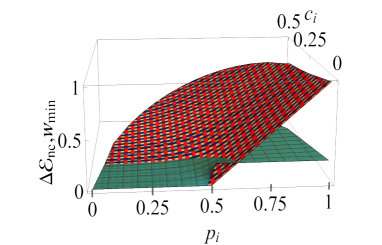
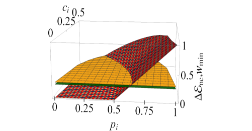
Figure 1: Top Panel: Plot of the energy gain $\Delta{\cal E}_{\rm nc}=G_{\rho_{i}}$ (texturised surface) and the energetic cost $w_{\rm min}$ (solid green surface) both in unit of $\hbar\lambda_{f}\omega$, in function of the initial population $p_{i}\in[0;1]$ and coherence $|c_{i}|\in[0;\sqrt{p_{i}(1-p_{i})}]$. We assume a driving velocity slower than the free evolution, setting $1/\tau=\lambda_{f}\omega/10$, which allows one to convert $\hbar/\tau$ in unit of $\hbar\lambda_{f}\omega$. Bottom Panel: Same plot with the upper bound $0.89\frac{\hbar\pi}{\tau}$ (yellow horizontal plane) and the lower bound $0.77\frac{\hbar\pi}{\tau}$ (green horizontal plane just below the yellow plane) of the average energetic cost $\overline{w_{\rm min}}$ (when no experimental control of the phases is available).

Illustrative examples.— So far, we showed that non-thermal features can be used to gain or save energy in driving operations. On the other hand, we also saw that there is an intrinsic energetic cost associated with optimal drives. Then, comes the following question: how large the energetic gains and the intrinsic energetic costs can be? We answer this question in two practical examples involving a two-level system. In the first example, we analyse the situation where $H_{i}$ is proportional to $H_{f}$ and compare the energetic gains provided by quantum coherences versus the energetic costs associated with the optimal drives. In the second example, we consider the more general situation where $H_{i}$ and $H_{f}$ are not proportional. Then, the bare dynamics $U_{0}(t)$ is not adiabatic and shortcuts-to-adiabaticity are needed in order to reach $\widetilde{(\rho_{i}^{\rm th})}_{f}$ when starting from a thermal state $\rho_{i}^{\rm th}$. Thus, in this second example, beyond evaluating the energetic gains provided by quantum coherences, we also compare the intrinsic energetic costs between the optimal drives and shortcut-to-adiabaticity.

Example 1.—We start by analysing the simple but common situation of a two-level system driven by a drive of the form $H_{0}(t):=\lambda(t)\hbar\frac{\omega}{2}\sigma_{z}$, which is naturally adiabatic since $[H_{0}(t),H_{0}(t^{\prime})]=0$ for all $t$ and $t^{\prime}$ Kosloff_2002 ; Feldmann_2003 . The time-dependent parameter takes the initial and final positive value $\lambda(t_{i}):=\lambda_{i}$ and $\lambda(t_{f}):=\lambda_{f}$, and $\sigma_{z}$ denotes the z-Pauli matrix, with $|1\rangle$ and $|0\rangle$ the excited and ground states, respectively. A general initial non-thermal state is of the form $\rho_{i}=\begin{pmatrix}p_{i}&c_{i}\\ c_{i}^{*}&1-p_{i}\\ \end{pmatrix}$ in the basis $\{|1\rangle,|0\rangle\}$. The associated non-cyclic ergotropy is given by (2) with the eigenvalues $r_{1}$ and $r_{0}$ functions of $c_{i}$ and $p_{i}$ (expressions detailed in Appendix E). The minimum energetic cost associated with the family of optimal drivings $V(t)$ is, according to the previous paragraph, given by $w_{\rm min}=\frac{\sqrt{2}\hbar}{\tau}{\rm arctan}\frac{p_{i}-r_{1}}{r_{0}-p_{i}}$.

On the other hand, the initial thermal state of same energy as $\rho_{i}$ is simply $\rho_{i}^{\rm th}={\rm diag}(p_{i},1-p_{i})$, and the original drive $H_{0}(t)$ is already adiabatic as commented above. Then, the energetic gain provided by the coherences $c_{i}$ is given by the non-cyclic ergotropy difference (3), which gives here

$$\Delta{\cal E}_{\rm nc} = \hbar\lambda_{f}\omega\left[\sqrt{\left(1/2-p_{i}\right)^{2}+|c_{i}|^{2}}-1/2+p_{i}\right]\geq 0,$$

and is also equal to the alternative figure of merit $G_{\rho_{i}}$.

Fig. 1 (a) presents a plot of $\Delta{\cal E}_{\rm nc}=G_{\rho_{i}}$ and $w_{\rm min}$ assuming a driving velocity slower than the free evolution, $1/\tau=\lambda_{f}\omega/10$. One can see that the energetic gain is always larger than the cost for large initial coherences, as long as $p_{i}\geq 0.025$ (obtained numerically, not visible on the figure). Note that, rigorously speaking, $\Delta{\cal E}_{\rm nc}$ becomes ill-defined for $p_{i}\geq 1/2$ because then $\rho_{i}^{\rm th}$ is not anymore passive (negative temperature). Still, we can use $G_{\rho_{i}}$ to consider the energetic gain beyond $p_{i}=1/2$. Then, the sudden step in the driving cost at $p_{i}=1/2$ happens because at this point the populations become inverted. This implies that, for $c_{i}=0$, optimal drives must swap the two eigenstates $|0\rangle$ and $|1\rangle$, whose cost is precisely $\frac{\pi\hbar}{\tau\sqrt{2}}$. If the experimental setup does not offer control of the phases $\phi_{1}$ and $\phi_{2}$, the average energetic cost $\overline{w_{\rm min}}$ takes value between $0.77\pi\frac{\hbar}{\tau}$ and $0.89\pi\frac{\hbar}{\tau}$, displayed in Fig. 1 (b).

(a)
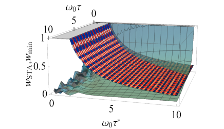
    (b)​​​​​​​​​​​​​​​​​
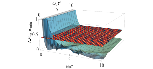
(c)

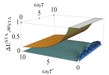
Figure 2: Plots of (a) $w_{\rm STA}$ (texturised surface) and $w_{\rm min}$ (blue solid surface); (b) $\Delta{\cal E}_{\rm nc}=G_{\rho_{i}}$ (horizontal texturised plane) and $w_{\rm min}$ (blue solid surface); and (c) $\Delta E^{\rm STA}$ (lower blue surface) and $w_{\rm STA}$ (upper yellow surface). All plots are in unit of $\hbar\omega_{0}$ and in function of $\omega_{0}\tau$ and $\omega_{0}\tau^{*}$, for $p_{i}=0.4$ and $c_{i}=\sqrt{0.4\times 0.6}$.

Example 2.—We consider now the same system but with $H_{i}:=\frac{1}{2}\hbar\omega_{0}\sigma_{z}$ and $H_{f}:=\frac{\hbar\omega_{f}}{2}\sigma_{z}+\frac{\hbar\epsilon_{f}}{2}\sigma_{x}$ not commuting, implying that $H_{0}(t)$ is necessarily non-adiabatic. We focus on the following family of driving, $H_{0}(t)=\frac{1}{2}\hbar\omega(t)\sigma_{z}+\frac{1}{2}\hbar\epsilon(t)\sigma_{x}$, with $\omega(t_{i})=\omega_{0}$, $\epsilon(t_{i})=0$, $\omega(t_{f})=\omega_{f}$, and $\epsilon(t_{f})=\epsilon_{f}$. In order to allow for analytic treatment of the dynamics, we assume that the time-dependent frequencies are such that $\mu:=\frac{\dot{\omega}(t)\epsilon(t)-\dot{\epsilon}(t)\omega(t)}{\Omega^{3}(t)}$ is constant Feldmann_2003 ; Dann_2020 , where $\Omega(t):=\sqrt{\omega^{2}(t)+\epsilon^{2}(t)}$. This includes for instance time dependent frequencies of the form $\omega(t)=\omega_{0}\cos[\pi(t-t_{i})/2\tau^{*}]$ and $\epsilon(t)=\omega_{0}\sin[\pi(t-t_{i})/2\tau^{*}]$, commonly used experimentally Peterson_2019 . Such choice implies $\mu=-\pi/(2\omega_{0}\tau^{*})$, $\omega_{f}=\omega_{0}\cos[\pi\tau/2\tau^{*}]$ and $\epsilon_{f}=\omega_{0}\sin[\pi\tau/2\tau^{*}]$, whose exact value will depend on one’s choice of $\tau^{*}$. In particular, for $\omega_{0}\tau^{*}\rightarrow\infty$, the adiabatic parameter Dann_2020 $\mu$ goes to zero, indicating adiabaticity, while $|\mu|\rightarrow\infty$ for $\omega_{0}\tau^{*}\rightarrow 0$, indicating strong non-adiabaticity.

Since $H_{0}(t)$ is non-adiabatic (at least for finite $\omega_{0}\tau$), optimal drives for initial thermal states $\rho_{i}^{\rm th}$ use shortcut-to-adiabaticity delCampo_2014 ; Deng_2013 ; Beau_2016 ; Abah_2019 ; Hartmann_2020 ; Dann_2020 ; Deng_2018 . It consists in adding an extra drive, like for instance the so-called counter-diabatic drive $V_{\rm CD}(t)$ Demirplak_2003 ; Demirplak_2005 ; Demirplak_2008 ; Berry_2009 , whose aim is to suppress generation of coherences and level transitions. Then, for an initial thermal state $\rho_{i}^{\rm th}=p_{i}|1\rangle\langle 1|+(1-p_{i})|0\rangle\langle 0|$, the addition of the counter-diabatic drive $V_{\rm CD}(t)$ yields the final passive state $\widetilde{(\rho_{i}^{\rm th})}_{f}:=p_{i}|e_{1}^{f}\rangle\langle e_{1}^{f}|+(1-p_{i})|e_{0}^{f}\rangle\langle e_{0}^{f}|$ (which happens to be also a thermal state since there is only two energy levels), and reaches the non-cyclic ergotropy equal to ${\cal E}_{\rm nc}^{\rm STA}=E_{i}-{\rm Tr}\left[\widetilde{(\rho_{i}^{\rm th})}_{f}H_{f}\right]$. The expression of $V_{\rm CD}(t)$ tailored for our problem is provided in Appendix F.2 (see also Feldmann_2003 ; Dann_2020 ) as well as the derivation of the associated energetic cost $w_{\rm STA}$ according to the criteria discussed above. We find $w_{\rm STA}=|\mu|\frac{\hbar\bar{\Omega}}{\tau}$, with $\bar{\Omega}:=\int_{t_{i}}^{t_{f}}dt\Omega(t)$.

It is also interesting to estimate how much energy is indeed gained or saved thanks to the shortcut-to-adiabaticity, and compare it to $w_{\rm STA}$. This requires to compute the energy of the final state $\rho_{f}$ we would obtain using only the bare drive $H_{0}(t)$. We obtain ${\rm Tr}(\rho_{f}H_{f})=\Omega_{f}(p_{f}-1/2)$, where $\Omega_{f}:=\Omega(t_{f})$ and $p_{f}=\langle e_{1}^{f}|\rho_{f}|e_{1}^{f}\rangle$ is the population in the final excited state (analytical expression provided in Appendix F). Thus, the energetic gain associated with the counter-adiabatic drive is $\Delta E^{\rm STA}:={\rm Tr}(\rho_{f}H_{f})-{\rm Tr}\left[\widetilde{(\rho_{i}^{\rm th})}_{f}H_{f}\right]=\hbar\Omega_{f}(\frac{1}{2}-p_{i})\frac{\mu^{2}(1-\nu_{c})}{1+\mu^{2}}$, with $\nu_{c}:=\cos\bar{\Omega}\sqrt{1+\mu^{2}}$. Note that the energetic gain $\Delta E^{\rm STA}$ is positive only for initial positive temperature ($p_{i}\leq 1/2$). This is because thermal states of negative temperature are non-passive, and then shortcut-to-adiabaticity techniques stop being optimal.

We now focus on the non-cyclic ergotropy achieved by an arbitrary non-passive state $\rho_{i}=\begin{pmatrix}p_{i}&c_{i}\\ c_{i}^{*}&1-p_{i}\\ \end{pmatrix}$ (in the initial eigenbasis). Using the family of optimal drives $V(t)$ we can achieve the optimal final state $\widetilde{(\rho_{i})}_{f}=r_{1}|e_{1}^{f}\rangle\langle e_{1}^{f}|+r_{0}|e_{0}^{f}\rangle\langle e_{0}^{f}|$, with the expressions of $r_{1}$ and $r_{0}$ as in the example 1. The energetic gain with respect to the performance of shortcut-to-adiabaticity technique applied to initial thermal states is $\Delta{\cal E}_{\rm nc}={\cal E}_{\rm nc}-{\cal E}_{\rm nc}^{\rm STA}=\hbar\Omega_{f}\left[\sqrt{(\frac{1}{2}-p_{i})^{2}+|c_{i}|^{2}}-(\frac{1}{2}-p_{i})\right]\geq 0$, same as in example 1, which is also equal to the alternative figure of merit $G_{\rho_{i}}$. However, differently from the example 1, one can now compare the energetic costs $w_{\rm STA}$ and $w_{\rm min}$, which provides a fairer comparison of performances between initial thermal states and non-passive states. The values taken by $w_{\rm min}$ now depends on some phases like the phase of the initial coherence $c_{i}$ (see technical details in Appendix F.1). We find that $w_{\rm min}$ belongs to the interval $\frac{\sqrt{2}\hbar}{\tau}|\theta_{1,{\rm min}}-\theta_{2,{\rm min}}|\leq w_{\rm min}\leq\frac{\sqrt{2}\hbar}{\tau}\pi$, where $\theta_{1,{\rm min}}:={\rm arctan}\sqrt{\frac{p_{i}-r_{1}}{r_{0}-p_{i}}}$ corresponds to the minimal energetic cost in example 1 and $\theta_{2,{\rm min}}:={\rm arctan}\frac{|\mu|\sqrt{1-\nu_{c}}}{\sqrt{2+\mu^{2}(1+\nu_{c})}}$ is only due to the non-adiabaticity of $U_{0}(\tau)$. Importantly, if one has experimental control of the phases, the minimal energetic cost $\frac{\sqrt{2}\hbar}{\tau}|\theta_{1,{\rm min}}-\theta_{2,{\rm min}}|$ can always be achieved.

In Fig. 2 (a), we compare these energetic costs providing a plot of $w_{\rm STA}$ for $p_{i}=0.4$ and $w_{\rm min}$ for $p_{i}=0.4$ and $c_{i}=\sqrt{0.4\times 0.6)}$. We use the specific form of the time dependent frequencies mentioned above, implying $\Omega(t)=\omega_{0}$, $\overline{\Omega}=\omega_{0}\tau$, and $w_{\rm STA}=\frac{\hbar\pi}{2\tau^{*}}$. Thus, the plots are in unit of $\hbar\omega_{0}$ and in function of $\omega_{0}\tau^{*}$, directly related to the level of non-adiabaticity, and $\omega_{0}\tau$, related to how fast is the driving with respect to the free evolution of the system. One can see that $w_{\rm min}$ is smaller than $w_{\rm STA}$ for most values of $\omega_{0}\tau$ and $\omega_{0}\tau^{*}$. In particular, while $w_{\rm STA}$ diverges for high non-adiabaticity, $w_{\rm min}$ remains finite. However, $w_{\rm min}$ diverges for very fast drives. Interestingly, one can show that this divergence of $w_{\rm min}$ is only due to the contribution from $\theta_{1,{\rm min}}$. In particular, for $c_{i}=0$, $w_{\rm min}$ remains finite and strictly smaller that $w_{\rm STA}$, meaning that the driving $V(t)$ is more performant than shortcut-to-adiabaticity.

In Fig. 2 (b), we compare the energetic gain $\Delta{\cal E}_{\rm nc}={\cal E}_{\rm nc}-{\cal E}_{\rm nc}^{\rm STA}$ (also equal to $G_{\rho_{i}}$) brought by the optimal drives with its energetic cost $w_{\rm min}$. In Fig. 2 (c), we compare the energetic gain $\Delta E^{\rm STA}$ brought by shortcut-to-adiabaticity with its energetic cost $w_{\rm STA}$. One can see that the performances of the optimal drives are significantly better than the performances of shortcut-to-adiabaticity. Additional plots in function of the more general parameters $\overline{\Omega}$ and $|\mu|$ are available in Appendix F.3, allowing us to conclude that the above tendency remain valid in more general settings.

Conclusion.— We initiate the exploration of energetic advantages in driving operations of quantum systems obtained from non-thermal states. These energetic advantages with respect to initial thermal states are captured by the non-cyclic ergotropy, composed by the sum of a coherent (coherence-based) contribution, an incoherent (population-based) contribution and a passive contribution. A more specific figure of merit can be introduced, $G_{\rho_{i}}$, focusing on the energetic gain brought by the optimal drive itself. It was shown to be equal to the non-cyclic ergotropy difference $\Delta{\cal E}_{\rm nc}$ for coherence-based non-passive states, as considered in the examples.

We saw that any non-thermal feature can bring energetic gains in the limit of many copies of the state. By contrast, for single state, we show, relying on majorization properties, that only quantum coherences can systematically bring energetic gains compared to initial thermal states. In particular, such gains are only achieved by dynamics able to consume coherences, emphasising the interplay between the presence of coherences and the ability to used them. It would be interesting to see if this mechanism could be the underlying phenomena behind the interferences effects enhancing the performance of cyclic engines pointed out in Camati_2019 , which would allow to extend its applications.

Additionally, the energetic costs associated with optimal drives can be significantly smaller than the ones associated with shortcut-to-adiabaticity technics while energetic gains can be significantly larger. Future investigations should be conducted to analyse other systems and potentially other criteria to evaluate the energetic costs of drives Abah_2019 .

All these energetic advantages rely on the availability of non-thermal states. There are indeed many realistic situations producing non-thermal states, including strong interaction with a thermal bath Smith_2014 ; Nazir_2018 , many-body systems interacting with a common bath Benatti_2003 ; Muschik_2011 ; Krauter_2011 ; PRR2019b ; Norcia_2018 ; minireview ; PRA2020 , non-Markovian evolution Zhang_2013 ; Addis_2014 , and interaction with several thermal baths at different temperatures Leggio_2015 .

Additional applications could be to explore questions suggested by our approach, like the lower energetic cost offered by the driving $V(t)$ compared to shortcut-to-adiabaticity, the tradeoff speed versus energetic cost of usual (cyclic) work extraction, as well as non-cyclic work extractions in quantum batteries. Finally, we anticipate direct applications in quantum engines operating with strong bath coupling Gelbwaser_2015 ; Newman_2017 ; Perarnau_2018 ; Newman_2020 ; Wiedmann_2020 or with structured bath Camati_2020 , where it has been reported mostly negative effects from the non-thermal properties and coherences naturally generated by these rich dynamics. A possible reason could be that such resources have not been fully exploited. Our results provide one possible direction.

Appendix A Incoherent and coherent non-adiabatic transformations

A.1 Non-adiabatic transformations

Any evolution leading to a passive state with respect to $H_{f}$ is necessarily non-adiabatic if and only if the initial state is a non-passive state with respect to $H_{i}$. This can be easily seen by writing the initial state in its diagonal form, $\rho_{i}=\sum_{n}r_{n}|r^{i}_{n}\rangle\langle r^{i}_{n}|$. The final state is passive if and only if the applied evolution $U$ satisfies the condition $\langle e_{n}^{f}|U|r_{n^{\prime}}\rangle=\delta_{n,n^{\prime}}$, where $\delta_{n,^{\prime}n}$ is the Kronecker delta. Then, if $\rho_{i}$ is a passive state, we have $|r_{n^{\prime}}\rangle=|e_{n^{\prime}}^{i}\rangle$ for all $n^{\prime}$, and the previous condition becomes $\langle e_{n}^{f}|U|e^{i}_{n^{\prime}}\rangle=\delta_{n,n^{\prime}}$, which corresponds to an adiabatic transformation, or more precisely, to an “integral or global” adiabatic transformation, a looser condition than a dynamics which is adiabatic at all intermediate times. By contrast, if $\rho_{i}$ is not passive, it means there exists at least one $n$ such that $|r^{i}_{n}\rangle\neq|e_{n}^{i}\rangle$, implying that there exists at least another index $m\neq n$ satisfying $\langle e^{i}_{m}|r^{i}_{n}\rangle\neq 0$. The condition for having a final passive state requires $\langle e_{n}^{f}|U|r_{n}\rangle=1$, implying in fine that $U$ contains the transition $|e_{n}^{f}\rangle\langle e_{m}^{i}|$, so that $U$ necessarily realises a non-adiabatic transformation.

A.2 Coherent and incoherent contributions

Non-thermal and non-passive features have two distinguished contributions: one from populations and one from coherences. It is possible to separate these two contributions in the non-cyclic ergotropy, extending similar considerations presented in Francica_2020 on ergotropy. However, for non-cyclic ergotropy, it is convenient to introduce a passive contribution, described in the following. For an initial state $\rho_{i}$, we denote by $\rho_{i|_{D}}:=\sum_{n}\langle e_{n}^{i}|\rho_{i}|e_{n}^{i}\rangle|e_{n}^{i}\rangle\langle e_{n}^{i}|$ the corresponding dephased state. The incoherent contribution to the non-cyclic ergotropy is ${\cal E}_{\rm nc}^{\rm inc}:={\rm Tr}(\rho_{i}H_{i})-{\rm Tr}\left[\widetilde{\rho_{i|_{D}}}H_{i}\right]$, where $\widetilde{\rho_{i|_{D}}}=\sum_{n}p^{i}_{\sigma(n)}|e_{n}^{i}\rangle\langle e_{n}^{i}|$ is the passive state of $\rho_{i|_{D}}$ with respect to $H_{i}$, with $p^{i}_{n}:=\langle e^{i}_{n}|\rho_{i}|e^{i}_{n}\rangle$ are the populations in the initial energy basis, and $\sigma(n)$ is a permutation of the indices such that $p^{i}_{\sigma(n+1)}\leq p^{i}_{\sigma(n)}$. Obviously, in the particular situation where the populations $p_{n}^{i}$ of $\rho_{i}$ are already in decreasing order we have $\widetilde{\rho_{i|_{D}}}=\rho_{i|_{D}}$ and the incoherent contribution is null since ${\rm Tr}(\rho_{i|_{D}}H_{i})={\rm Tr}(\rho_{i}H_{i})$. By defining the unitary transformation $U_{\sigma}:=\sum_{n}e^{i\psi_{n}}|e^{i}_{n}\rangle\langle e^{i}_{\sigma(n)}|$, where $\psi_{n}$ is a phase factor, we obtain $\widetilde{\rho_{i|_{D}}}=U_{\sigma}\rho_{i|_{D}}U_{\sigma}^{{\dagger}}=\left(U_{\sigma}\rho_{i}U_{\sigma}^{{\dagger}}\right)_{|_{D}}$. Alternatively, $\widetilde{\rho_{i|_{D}}}$ can be defined as Francica_2020 $\widetilde{\rho_{i|_{D}}}={\rm argmin}_{\sigma\in{\cal S}^{\rm inc}}{\rm Tr}(\sigma H_{i})$, where ${\cal S}^{\rm inc}:=\{U_{\xi}\rho_{i|_{D}}U_{\xi}^{{\dagger}}\}_{U_{\xi}\in{\cal U}^{\rm inc}}$ and ${\cal U}^{\rm inc}$ denotes the ensemble of incoherent unitary transformations with respect to the initial energy eigenbasis. Incoherent unitaries are of the form $\sum_{n}e^{i\Theta_{n}}|e^{i}_{n}\rangle\langle e_{\xi(n)}^{i}|$, where $\xi(n)$ is a permutation of the indices and $\Theta_{n}$ a phase factor. Importantly, ${\cal E}_{\rm nc}^{\rm inc}$ is always positive.

The second contribution is the passive one, defined as ${\cal E}_{\rm nc}^{\rm pas}:={\rm Tr}\left[\widetilde{\rho_{i|_{D}}}H_{i}\right]-{\rm Tr}\left[\widetilde{(\rho_{i|_{D}})}_{f}H_{f}\right]$ with $\widetilde{(\rho_{i|_{D}})}_{f}:=\sum_{n}p^{i}_{\sigma(n)}|e_{n}^{f}\rangle\langle e_{n}^{f}|$ is the passive state of $\rho_{i|_{D}}$ with respect to $H_{f}$. Note that $\widetilde{(\rho_{i|_{D}})}_{f}$ is related to $\widetilde{\rho_{i|_{D}}}$ through adiabatic transformations which are of the form $U_{\rm ad}=\sum_{n}e^{i\phi_{n}}|e_{n}^{f}\rangle\langle e_{n}^{i}|$. Additionally, ${\cal E}_{\rm nc}^{\rm pas}$ can be positive or negative.

The coherent contribution to the non-cyclic ergotropy can be defined as ${\cal E}_{\rm nc}^{\rm coh}={\rm Tr}\left[\widetilde{(\rho_{i|_{D}})}_{f}H_{f}\right]-{\rm Tr}\left[\widetilde{(\rho_{i})}_{f}H_{f}\right]$. ${\cal E}_{\rm nc}^{\rm coh}$ is always positive since ${\rm Tr}\left[\widetilde{(\rho_{i|_{D}})}_{f}H_{f}\right]={\rm Tr}\left[U_{\rm ad}U_{\sigma}\rho_{i}U_{\sigma}^{{\dagger}}U_{\rm ad}^{{\dagger}}H_{f}\right]$ and $\widetilde{(\rho_{i})}_{f}$ is the passive state associated with $\rho_{i}$ but also to $U_{\rm ad}U_{\sigma}\rho_{i}U_{\sigma}^{{\dagger}}U_{\rm ad}^{{\dagger}}$. A similar expression as in Francica_2020 can be obtained for the coherent non-cyclic ergotropy:

$${\cal E}_{\rm nc}^{\rm coh}=\beta^{-1}\left[{\cal C}(\rho_{i})+S[\widetilde{(\rho_{i|_{D}})}_{f}|\rho_{f}^{\rm th}(\beta)]-S[\widetilde{(\rho_{i})}_{f}|\rho_{f}^{\rm th}(\beta)]\right]$$

where $\rho_{f}^{\rm th}(\beta)$ denotes a thermal state of the final Hamiltonian at arbitrary inverse temperature $\beta$, and ${\cal C}(\rho_{i})=S[\rho_{i|_{D}}]-S[\rho_{i}]$ is the amount of initial coherences measured with the relative entropy of coherence Baumgratz_2014 . While $\widetilde{(\rho_{i|_{D}})}_{f}$ can be reached by incoherent non-adiabatic evolutions, for instance $U_{\rm ad}U_{\sigma}$, $\widetilde{(\rho_{i})}_{f}$ can be reached only via coherent non-adiabatic evolutions. It can be easily seen by remembering that applying an incoherent non-adiabatic evolution to an initial state containing coherences necessarily yields a final state with coherences. Alternatively, one can see it by noticing that an evolution able to consume coherences is also able to generate coherences.

Finally, the three contributions add up to give the non-cyclic ergotropy: ${\cal E}_{\rm nc}={\cal E}^{\rm inc}_{\rm nc}+{\cal E}^{\rm pas}_{\rm nc}+{\cal E}^{\rm coh}_{\rm nc}$. Note that the passive contribution can alternatively be defined before the incoherent one or after the coherent one. This could in general change the respective value of each contribution but without changing their nature.

A.3 Consequences for energetic gain

The above decomposition of ${\cal E}_{\rm nc}$ is insightful to understand the difference between coherence and population-based non-passivity. For coherence-based non-passivity, the energetic gain, given by the difference of non-cyclic ergotropy (Eq.3 of the main text), can be decomposed as

$$\Delta{\cal E}_{\rm nc} = {\cal E}_{\rm nc}(\rho_{i})-{\cal E}_{\rm nc}(\rho_{i}^{\rm th})$$ (10)

$$= {\cal E}_{\rm nc}^{\rm pas}(\rho_{i})+{\cal E}_{\rm nc}^{\rm coh}(\rho_{i})-{\cal E}_{\rm nc}^{\rm pas}(\rho_{i}^{\rm th}).$$

Since we assumed that $\rho_{i}$ contains only coherence-based non-passive features, the populations are the same as the thermal state $\rho_{i}^{\rm th}$ of same energy, and consequently the passive contributions are also the same, ${\cal E}_{\rm nc}^{\rm pas}(\rho_{i})={\cal E}_{\rm nc}^{\rm pas}(\rho_{i}^{\rm th})$. Consequently,

$$\Delta{\cal E}_{\rm nc} = {\cal E}_{\rm nc}^{\rm coh}(\rho_{i})\geq 0,$$ (11)

from which we conclude that coherences always bring energetic gains.

By contrast, for a population-based non-passive state, the populations can be very different from the thermal state of same energy, so that the passive contributions can be very different too. Then, we have

$$\Delta{\cal E}_{\rm nc} = {\cal E}_{\rm nc}^{\rm pas}(\rho_{i})+{\cal E}_{\rm nc}^{\rm inc}(\rho_{i})-{\cal E}_{\rm nc}^{\rm pas}(\rho_{i}^{\rm th})$$ (12)

$$= \Delta{\cal E}_{\rm nc}^{\rm pas}+{\cal E}_{\rm nc}^{\rm inc}(\rho_{i}),$$

which can be of any sign since $\Delta{\cal E}_{\rm nc}^{\rm pas}:={\cal E}_{\rm nc}^{\rm pas}(\rho_{i})-{\cal E}_{\rm nc}^{\rm pas}(\rho_{i}^{\rm th})$ can be positive or negative. This is illustrated in the next section with three-level systems.

Appendix B Larger non-cyclic work extraction from passive states than from non-passive states

In this Appendix we provide explicit example that for non-cyclic transformations, initial passive states can yield a larger work extraction (for positive non-cyclic ergotropy) or require less driving energy (for negative non-cyclic ergotropy) than non-passive states. We consider a three-level system and a non-cyclic process with initial Hamiltonian $H_{i}=\sum_{n=1}^{3}e_{n}^{i}|e_{n}^{i}\rangle\langle e_{n}^{i}|$ and the final Hamiltonian $H_{f}=\sum_{n=1}^{3}e_{n}^{f}|e_{n}^{f}\rangle\langle e_{n}^{f}|$. Without loss of generality, we assume that $e^{i}_{1}=e^{f}_{1}=0$ and $e^{i}_{3}=e^{f}_{3}=1$, which implies that $e_{2}^{i}$ and $e_{2}^{f}$ belong to the interval $[0;1]$. As passive state, we consider a thermal state $\rho_{i}^{\rm th}$ at inverse temperature $\beta$. We denote by $p_{n}^{\rm th}$ its initial populations associated with the eigenvector $|e_{n}^{i}\rangle$. We are looking for a non-passive state such that its non-cyclic ergotropy is strictly smaller than the one of the thermal state. Since we saw in the main text that initial coherences always increase the non-cyclic ergotropy, we choose a diagonal non-passive state $\rho_{i}=\sum_{n=1}^{3}q_{i}|e_{n}^{i}\rangle\langle e_{n}^{i}|$. In other words, we need to find $q_{1}$, $q_{2}$, and $q_{3}$ such that $\widetilde{E}_{f}=q^{*}_{3}+q^{*}_{2}e_{2}^{f}>{\rm Tr}\left[\widetilde{(\rho_{i}^{\rm th})}_{f}H_{f}\right]=p_{3}^{\rm th}+p_{2}^{\rm th}e_{2}^{f}$, remembering that $\widetilde{(\rho_{i}^{\rm th})}_{f}$ is the final passive state associated with $\rho_{i}^{\rm th}$. We introduced $q_{3}^{*}:={\rm min}_{n=1,2,3}~{}q_{n}$ and $q_{2}^{*}$ is the second smallest population.

One can show for instance that choosing $e_{2}^{i}$ such that $\beta(1-e_{2}^{i})\ll 1$, with $q_{3}=p_{3}^{\rm th}+\alpha$, $q_{2}=p_{2}^{\rm th}-\alpha/e_{2}^{i}$, and $q_{1}=1-q_{2}-q_{3}$, where $\alpha:=e^{-\beta}\beta(e_{2}^{i}-(e_{2}^{i})^{2})/3$ guarantees $q_{3}^{*}>p_{3}^{\rm th}$. This implies that we can always have $\widetilde{E}_{f}>{\rm Tr}\left[\widetilde{(\rho_{i}^{\rm th})}_{f}H_{f}\right]$ by choosing $e_{2}^{f}$ small enough.

Explicitly, let us take $\beta=1$ (in unit of $k_{B}$) and $e_{2}^{i}=0.9$. With these values we obtain according to the above choices $p_{1}^{\rm th}\simeq 0.564$, $p_{2}^{\rm th}\simeq 0.229$, $p_{3}^{\rm th}\simeq 0.207$, $q_{1}\simeq 0.565$, $q_{2}\simeq 0.217$, and $q_{3}\simeq 0.218$. Thus, we have for the final populations $q_{3}^{*}-p_{3}^{\rm th}=q_{3}-p_{3}^{\rm th}\simeq 0.00954$ and $p_{2}^{\rm th}-q_{2}^{*}=p_{2}^{\rm th}-q_{3}=0.0108$, so that any value of $e_{2}^{f}$ smaller than $0.88$ leads to $\widetilde{E}_{f}>{\rm Tr}\left[\widetilde{(\rho_{i}^{\rm th})}_{f}H_{f}\right]$.

Appendix C Asymptotic achievability of the upper bound Eq.(7)

The theorem shown in Alicki_2013 states that for any state $\rho$ and for $N$ going to infinity, there exists a unitary transformation $U_{N}$ (not unique) such that

$$\frac{1}{N}{\rm Tr}\left(U_{N}\otimes^{N}\rho U_{N}^{{\dagger}}H_{N}\right)\underset{N\rightarrow\infty}{\rightarrow}{\rm Tr}(\rho^{\rm th}H),$$ (13)

where $H$ can be an arbitrary Hamiltonian, $H_{N}:=\sum_{k=0}^{N-1}\otimes^{k}\mathbb{I}\otimes H\otimes^{N-k-1}\mathbb{I}$, $\mathbb{I}$ is the identity, and $\rho^{\rm th}$ is the thermal state of same entropy as $\rho$ associated with the Hamiltonian $H$. Then, it implies the existence of a unitary transformation mapping asymptotically well (in the sense stated above) $\otimes^{N}\rho_{i}$ to $\otimes^{N}(\rho_{i})_{f}^{\rm th}$, remembering that $(\rho_{i})_{f}^{\rm th}$ denotes the thermal state with respect to $H_{f}$ of same entropy as $\rho_{i}$. In particular, it also means that we can find a time dependent Hamiltonian $H_{N}(t)$ such that the generated unitary transformation realises this mapping with the additional constraints $H_{N}(t_{i})=\sum_{k=0}^{N-1}\otimes^{k}\mathbb{I}\otimes H_{i}\otimes^{N-k-1}\mathbb{I}$ and $H_{N}(t_{f})=\sum_{k=0}^{N-1}\otimes^{k}\mathbb{I}\otimes H_{f}\otimes^{N-k-1}\mathbb{I}$.

Appendix D Optimal drivings

One can verify easily that the family of driving $V(t)$ given in the main text brings the initial state $\rho_{i}$ to the optimal final state $\tilde{\rho}_{f}$. The complete transformation is given by

$$U = e^{-i{\cal T}\int_{t_{i}}^{t_{f}}dtH(t)}$$ (14)

$$= e^{-i{\cal T}\int_{t_{i}}^{t_{f}}dtH_{0}(t)}$$

$$\times e^{-i{\cal T}\int_{t_{i}}^{t_{f}}dte^{i{\cal A}\int_{t_{i}}^{t}duH_{0}(u)}V(t)e^{-i{\cal T}\int_{t_{i}}^{t}duH_{0}(u)}}$$

$$= e^{-i{\cal T}\int_{t_{i}}^{t_{f}}dtH_{0}(t)}e^{i\chi\int_{t_{i}}^{t_{f}}dt\dot{f}(t)}$$

$$= e^{-i{\cal T}\int_{t_{i}}^{t_{f}}dtH_{0}(t)}e^{i\chi[f(t_{f})-f(t_{i})]}$$

$$= \sum_{n}e^{i\phi_{n}}|e_{n}^{f}\rangle\langle r^{i}_{n}|,$$

where we used the definition of $\chi$ and the properties $f(t_{i})=0$ and $f(t_{f})=1$. It is then straightforward to see that $U$ brings $\rho_{i}$ to the optimal final state.

Appendix E Details on the energetic cost of driving for two-level systems

The eigenvalues and eigenvectors associated with the initial state $\rho_{i}=\begin{pmatrix}p_{i}&c_{i}\\ c_{i}^{*}&1-p_{i}\\ \end{pmatrix}$ are respectively

$$r_{1}=\frac{1}{2}-\sqrt{(p_{i}-1/2)^{2}+|c_{i}|^{2}},$$ (15)

$$r_{0}=\frac{1}{2}+\sqrt{(p_{i}-1/2)^{2}+|c_{i}|^{2}},$$ (16)

and

$$|r_{1}\rangle=\sqrt{\frac{r_{0}-p_{i}}{r_{0}-r_{1}}}|1\rangle-e^{-i\psi_{i}}\sqrt{\frac{p_{i}-r_{1}}{r_{0}-r_{1}}}|0\rangle,$$ (17)

$$|r_{0}\rangle=e^{i\psi_{i}}\sqrt{\frac{p_{i}-r_{1}}{r_{0}-r_{1}}}|1\rangle+\sqrt{\frac{r_{0}-p_{i}}{r_{0}-r_{1}}}|0\rangle,$$ (18)

where $\psi_{i}={\rm arg}(c_{i})$. The unitary evolution $U_{0}(t)$ is simply given by $U_{0}(t)=e^{-i\Lambda\frac{\omega}{2}\sigma_{z}}$, with $\Lambda:=\int_{t_{0}}^{t_{f}}dt\lambda(t)$. Since both $H_{i}$ and $H_{f}$ are proportional to $\sigma_{f}$, the initial and final energy eigenstates are the same, namely $|1\rangle$ and $|0\rangle$. As detailed in the main text, optimal drivings can be obtained through the matrix $\chi$ which is itself given by

$$e^{i\chi} = \sum_{n}e^{i\phi_{n}}U_{0}^{{\dagger}}(t_{f})|e^{f}_{n}\rangle\langle r^{i}_{n}|$$ (19)

$$= e^{i\phi_{1}}e^{i\Lambda\frac{\omega}{2}}|1\rangle\langle r_{1}|+e^{i\phi_{0}}e^{-i\Lambda\frac{\omega}{2}}|0\rangle\langle r_{0}|.$$

The associated eigenvalues are $e^{i\theta_{+}}$ and $e^{i\theta_{-}}$ with

$$\theta_{\pm} = \frac{\phi_{0}+\phi_{1}}{2}+\pi\kappa(\phi_{1}-\phi_{0})$$ (21)

$$\pm{\rm arctan}\sqrt{\frac{r_{0}-r_{1}}{(r_{0}-p_{i})\cos^{2}{(\phi_{1}-\phi_{0})/2}}-1},$$

where $\kappa(\phi_{1}-\phi_{0})$ is a function equal to 0 when $\cos(\phi_{1}-\phi_{0})\geq 0$ and equal to 1 otherwise (explicitly, $\kappa(\phi_{1}-\phi_{0})=\Theta[-\cos(\phi_{1}-\phi_{0})]$, where $\Theta$ is the Heaviside step function). Assuming one has full control of the phases, one can achieve the following minimal energetic cost

$$w_{\rm min} = \frac{\sqrt{2}}{\tau}{\rm arctan}\sqrt{\frac{p_{i}-r_{1}}{r_{0}-p_{i}}}$$

$$= \frac{\sqrt{2}}{\tau}{\rm arctan}\left(\frac{\sqrt{(1/2-p_{i})^{2}+|c|^{2}}-(1/2-p_{i})}{\sqrt{(1/2-p_{i})^{2}+|c|^{2}}+(1/2-p_{i})}\right)^{1/2},$$

by setting $\phi_{1}=\phi_{0}=0$. By contrast, if one has no control of the phases, their value for each realisation is random, and the average cost is given by

$$\bar{w}:=\frac{1}{\tau}\frac{1}{4\pi^{2}}\int_{-\pi}^{\pi}d\phi_{1}\int_{-\pi}^{\pi}d\phi_{2}~{}\sqrt{\theta_{+}^{2}+\theta_{-}^{2}}.$$ (23)

The analytical expression is challenging to obtain, but one can instead show that $\frac{1}{4\pi^{2}}\int_{-\pi}^{\pi}d\phi_{1}\int_{-\pi}^{\pi}d\phi_{2}~{}\sqrt{\theta_{+}^{2}+\theta_{-}^{2}}$ takes value within the interval $[0.77\pi;0.89\pi]$ depending on the values of $p_{i}$ and $c_{i}$.

Appendix F Non-adiabatic dynamics

The time dependent Hamiltonian considered in the last part of the paper is of the form

$$H_{0}(t)=\frac{1}{2}\omega(t)\sigma_{z}+\frac{1}{2}\epsilon(t)\sigma_{x},$$ (24)

and generates a non-adiabatic dynamics since $[H(t),H(t^{\prime})]\neq 0$ in general. Such kind of dynamics are challenging to integrate. Still, analytical integrations are possible when the Hamiltonian parameters are such that $\mu:=\frac{\dot{\omega}(t)\epsilon(t)-\dot{\epsilon}(t)\omega(t)}{\Omega^{3}(t)}$ is constant Feldmann_2003 ; Dann_2020 . A simple way to integrate the dynamics is using a closed set of orthogonal observables $\{B_{k}\}_{0\leq k\leq 3}$ forming a basis of the Hilbert space. We use the same set as in Feldmann_2003 ; Dann_2020 , namely $B_{0}=\mathbb{I}$, $B_{1}=H_{0}(t)=\omega(t)S_{z}+\epsilon(t)S_{x}$, $B_{1}=\epsilon(t)S_{z}-\omega(t)S_{x}$, and $B_{3}=\Omega(t)S_{y}$. In the Heisenberg picture $B_{i}(t):=e^{i{\cal A}\int_{t_{i}}^{t}duH_{0}(u)}B_{i}e^{-i{\cal T}\int_{t_{i}}^{t}duH_{0}(u)}$ the dynamics is given by $\dot{B}_{i}(t)=i[H_{0}^{*}(t),B_{i}(t)]+\frac{\partial}{\partial t}B_{i}(t)$, where $H_{0}^{*}(t):=e^{i{\cal A}\int_{t_{i}}^{t}duH_{0}(u)}H_{0}e^{-i{\cal T}\int_{t_{i}}^{t}duH_{0}(u)}$ and the partial derivative denotes the derivative with respect to the intrinsic time-dependence of the operator $B_{i}$. The dynamics of the basis can be written in a matrix form

$$\frac{1}{\Omega}\dot{X}(t)=\left(A+\frac{\dot{\Omega}}{\Omega^{2}}\mathbb{I}\right)X(t)$$ (25)

where $X(t)=\{B_{1}(t),B_{2}(t),B_{3}(t)\}^{\rm T}$ is a three-component column vector and

$$A=\begin{pmatrix}0&\mu&0\\ -\mu&0&1\\ 0&-1&0\end{pmatrix}$$ (26)

a $3\times 3$-matrix. This can be integrated after diagonalising $A$, yielding (see also Feldmann_2003 ; Dann_2020 )

$$X(t)=\frac{\Omega(t)}{(\mu^{2}+1)\Omega(0)}\begin{pmatrix}1+\mu^{2}\nu_{c}&\mu\nu_{s}\sqrt{\mu^{2}+1}&(1-\nu_{c})\mu\\ -\mu\nu_{s}\sqrt{\mu^{2}+1}&\nu_{c}(\mu^{2}+1)&\nu_{s}\sqrt{\mu^{2}+1}\\ \mu(1-\nu_{c})&-\nu_{s}\sqrt{\mu^{2}+1}&\mu^{2}+\nu_{c}\end{pmatrix}X(0),$$ (27)

with $\nu_{c}:=\cos\bar{\Omega}\sqrt{1+\mu^{2}}$, $\nu_{s}:=\sin\bar{\Omega}\sqrt{1+\mu^{2}}$, and $\bar{\Omega}:=\int_{t_{i}}^{t_{f}}dt\Omega(t)$. Note that from $B_{i}(t)$ we have directly the expressions of $S_{z}(t)$, $S_{y}(t)$, and $S_{x}(t)$, from which we obtain the time dependent Bloch vector to reconstruct the final state, $\rho_{f}=\begin{pmatrix}p_{f}&c_{f}\\ c_{f}^{*}&1-p_{f}\\ \end{pmatrix}$ in the basis $\{|e_{1}^{f}\rangle,|e_{0}^{f}\rangle\}$. We obtain $p_{f}=\frac{1}{2(1+\mu^{2})}[2p_{i}+\mu^{2}-\mu^{2}\nu_{c}(1-2p_{i})]$ and $c_{f}=-\frac{\mu(1-2p_{i})}{2(1+\mu^{2})}{\rm sign}(\epsilon_{f})[\nu_{s}\sqrt{1+\mu^{2}}-i(1-\nu_{c})]$. The final eigenstates are given by $|e_{1}^{f}\rangle=[(\omega_{f}+\Omega_{f})^{2}+\epsilon_{f}^{2}]^{-1/2}[(\omega_{f}+\Omega_{f})|1\rangle+\epsilon_{f}|0\rangle]$ and $|e_{0}^{f}\rangle=[(\omega_{f}-\Omega_{f})^{2}+\epsilon_{f}^{2}]^{-1/2}[(\omega_{f}-\Omega_{f})|1\rangle+\epsilon_{f}|0\rangle]$.

F.1 Energetic cost of the family of optimal drive

The minimal energetic cost of an optimal drive is given by (see main text) $w_{\rm min}=\frac{1}{\tau}[{\rm Tr}\chi\chi^{{\dagger}}]^{1/2}$, where $\chi$ is such that $e^{i\chi}=\sum_{n}e^{i\xi_{n}}|e_{n}^{i}\prime\rangle\langle r^{i}_{n}|$. The expression of $|r_{1}\rangle$ and $|r_{0}\rangle$ are the same as in (17) and (18) respectively. We can derive the expression of $|e_{1}^{i}\prime\rangle$ and $|e_{0}^{i}\prime\rangle$ (up to a phase factor included in $\xi_{n}$) from the above expression of $\rho_{f}$, taking respectively $|1\rangle\langle 1|$ and $|0\rangle\langle 0|$ as initial state. We obtain

$$|e_{1}^{i}\prime\rangle=\alpha e^{-i\phi_{\alpha}}|1\rangle-\beta|0\rangle$$ (28)

$$|e_{0}^{i}\prime\rangle=\beta|1\rangle+\alpha e^{i\phi_{\alpha}}\beta|0\rangle$$ (29)

with $\alpha e^{i\phi_{\alpha}}=\frac{1}{\sqrt{2(1+\mu^{2})}}[{\rm sign}(s)\sqrt{(1+\mu^{2})(1+\nu_{c})}-i\sqrt{1-\nu_{c}}]$ and $\beta=\frac{1}{\sqrt{2(1+\mu^{2})}}{\rm sign}(\epsilon_{f})\mu\sqrt{1-\nu_{c}}$.

Combining with (28) and (29) with (17) and (18) we have

$$\sum_{n}e^{i\phi_{n}}|e_{n}^{i}\prime\rangle\langle r^{i}_{n}|=\begin{pmatrix}\cos\eta e^{i\zeta}&\sin\eta e^{-i(\delta-\xi_{1}-\xi_{0})}\\ -\sin\eta e^{i\delta}&\cos\eta e^{-i(\zeta-\xi_{0}-\xi_{1})}\\ \end{pmatrix}$$

in the initial energy eigenbasis $\{|1\rangle,|0\rangle\}$ with $\eta$, $\zeta$, and $\delta$ are implicitly defined by the relations $\cos\eta e^{i\zeta}=\alpha\sqrt{\frac{r_{0}-p_{i}}{r_{0}-r_{1}}}e^{i(\xi_{1}-\phi_{\alpha})}+\beta\sqrt{\frac{p_{i}-r_{1}}{r_{0}-r_{1}}}e^{i(\xi_{0}-\psi_{i})}$ and $\sin\eta e^{i\delta}=\beta\sqrt{\frac{r_{0}-p_{i}}{r_{0}-r_{1}}}e^{i\xi_{1}}-\alpha\sqrt{\frac{p_{i}-r_{1}}{r_{0}-r_{1}}}e^{i(\xi_{0}+\phi_{\alpha}-\psi_{i})}$, reminding that $\psi_{i}$ is the argument of the initial coherence $c_{i}$. As a result, the eigenvalues of $e^{i\chi}$ are $e^{i\theta_{+}}$ and $e^{i\theta_{-}}$ with

$$\theta_{\pm} = \frac{\xi_{1}+\xi_{0}}{2}+\pi\kappa(\xi_{1},\xi_{0},\alpha,\eta)\pm{\rm arctan}\sqrt{\frac{1}{\left[\alpha\sqrt{\frac{r_{0}-p_{i}}{r_{0}-r_{1}}}\cos(\phi_{\alpha}-\xi_{1}/2+\xi_{0}/2)+\beta\sqrt{\frac{p_{i}-r_{1}}{r_{0}-r_{1}}}\cos(\psi_{i}+\xi_{1}/2-\xi_{0}/2)\right]^{2}}-1},$$

where $\kappa(\xi_{1},\xi_{0},\alpha,\eta)$ is a function equal to 0 when $\cos\eta\cos(\zeta-\xi_{1}/2-\xi_{0}/2)\geq 0$, and equal to 1 otherwise. Assuming one has control of the phase $\xi_{1}$ and $\xi_{0}$, the minimum energetic cost is

$$w_{\rm min}=\frac{\sqrt{2}}{\tau}{\rm arctan}\sqrt{\left[\alpha^{2}\frac{r_{0}-p_{i}}{r_{0}-r_{1}}+\beta^{2}\frac{p_{i}-r_{1}}{r_{0}-r_{1}}+2\beta\alpha\frac{\sqrt{(r_{0}-p_{i})(p_{i}-r_{1})}}{r_{0}-r_{1}}\cos(\psi_{i}+\phi_{\alpha})\right]^{-1}-1}.$$ (32)

Contrasting with the first situation where $H_{0}(t)$ generates an adiabatic transformation, the energetic cost after minimisation over $\xi_{1}$ and $\xi_{0}$ depends on $\psi_{i}$, the initial phase of the coherence $c_{i}$, and on $\phi_{\alpha}$ (which depends on the original dynamics $U_{0}(t_{f})$). Then, one can consider again the same alternative. If experimentally one has control of these phases, meaning that they have well-defined values which can be adjusted by some controls on the experimental apparatus, then, the minimum energetic cost can be brought down to (for $\psi_{i}+\phi_{\alpha}=0$ if $\epsilon_{f}\mu\geq 0$, and for $\psi_{i}+\phi_{\alpha}=\pi$ if $\epsilon_{f}\mu\leq 0$)

$$w_{\rm min} = \frac{\sqrt{2}}{\tau}|\theta_{1,{\rm min}}-\theta_{2,{\rm min}}|,$$ (33)

with $\theta_{1,{\rm min}}={\rm arctan}\sqrt{\frac{p_{i}-r_{1}}{r_{0}-p_{i}}}$, contribution form the initial state, and $\theta_{2,{\rm min}}={\rm arctan}\frac{|\beta|}{\alpha}={\rm arctan}\frac{|\mu|\sqrt{1-\nu_{c}}}{\sqrt{2+\mu^{2}(1+\nu_{c})}}$, contribution from the original dynamics $U_{0}(t_{f})$. Conversely, if one has no control over $\psi_{i}$ and $\phi_{\alpha}$, the energetic cost can take any value between $\frac{\sqrt{2}}{\tau}|\theta_{1,{\rm min}}-\theta_{2,{\rm min}}|$ and $\frac{\sqrt{2}}{\tau}(\theta_{1,{\rm min}}+\theta_{2,{\rm min}})$.

Finally, without any control one the phases $\xi_{1}$ and $\xi_{0}$ and therefore left random, the energetic cost takes values between $\frac{\sqrt{2}}{\tau}|\theta_{1,{\rm min}}-\theta_{2,{\rm min}}|$ and $\frac{\sqrt{2}}{\tau}\pi$.

F.2 Counterdiabatic driving and energetic cost

According to Demirplak_2003 ; Demirplak_2005 ; Demirplak_2008 ; Berry_2009 , for a given time dependent Hamiltonian $H(t)$, the counterdiabatic drive is given by

$$H_{\rm CD}=\sum_{n}\left(\frac{d}{dt}\pi_{n}\right)\pi_{n}$$ (34)

where $\pi_{n}:=|e_{n}\rangle\langle e_{n}|$ are projectors onto the instantaneous eigenstates $|e_{n}\rangle$ of $H(t)$. The corresponding energetic cost is given by the time average of the Hamiltonian norm $||H(t)||$. One obtains $||H(t)||=\big{(}\sum_{n}\dot{\langle e_{n}}\dot{|e_{n}\rangle}\big{)}^{1/2}$, using the property $\dot{\langle e_{n}|}|e_{n}\rangle=0$, where $\dot{|e_{n}\rangle}$ stands for $\frac{d}{dt}|e_{n}\rangle$. Recalling that we consider the family of driving $H_{0}(t)=\frac{\omega(t)}{2}\sigma_{z}+\frac{\epsilon(t)}{2}\sigma_{x}$, the instantaneous eigenstates are given by

$$|e_{1}\rangle=\sqrt{\frac{\Omega(t)+\omega(t)}{2\Omega(t)}}|1\rangle+\sqrt{\frac{\Omega(t)-\omega(t)}{2\Omega(t)}}|0\rangle$$ (35)

and

$$|e_{0}\rangle=-\sqrt{\frac{\Omega(t)-\omega(t)}{2\Omega(t)}}|1\rangle+\sqrt{\frac{\Omega(t)+\omega(t)}{2\Omega(t)}}|0\rangle.$$ (36)

This leads to $||H(t)||=\frac{|\dot{\omega}(t)\epsilon(t)-\omega(t)\dot{\epsilon}(t)|}{\Omega^{2}(t)}=|\mu|\Omega(t)$, implying that the energetic cost is $w_{\rm STA}=|\mu|\bar{\Omega}/\tau$.

(a)​​​​​​​​​​​​​​​​
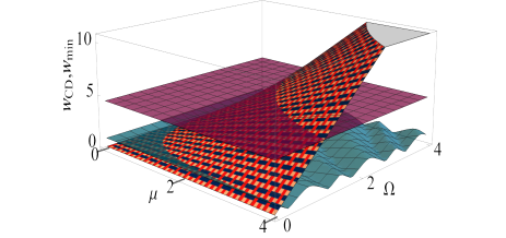
(b)​​​​​​​​​​​​​​​​​​​​​​​​​​​​
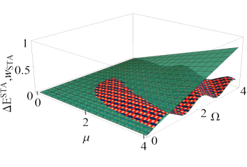
(c)​​​​​​​​​​​​​​​​​​​​​​​​​​​​

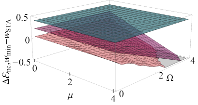
Figure 3: (a) Plot of $w_{\rm STA}$ (texturised surface) and $w_{\rm min}$ (blue solid lower surface) in unit of $\hbar/\tau$, in function of the dimensionless parameters $\mu\in[0;4]$ and $\bar{\Omega}\in[0;4]$, for $p_{i}=0.4$ and $c_{i}=\sqrt{0.4\times 0.6}$. The purple upper plane is the upper bound of $w_{\rm min}$ equal to $\pi\sqrt{2}$. (b) Plot of $w_{\rm STA}$ (green solid surface) and $\Delta E^{\rm STA}$ (texturised surface), both in unit of $\hbar\Omega_{f}$, in function of $\mu\in[0;4]$ and $\bar{\Omega}\in[0;4]$, assuming $\Omega_{f}=20/\tau$, which allows to convert $\hbar/\tau$ in unit of $\hbar\Omega_{f}$. (c) Plot of $w_{\rm min}-w_{\rm STA}$ (pink lower surface) and $\Delta{\cal E}_{\rm nc}$ (upper blue horizontal plane), both in unit of $\hbar\Omega_{f}$, in function of $\mu\in[0;4]$ and $\bar{\Omega}\in[0;4]$, still assuming $\Omega_{f}=20/\tau$. The purple intermediate surface is the upper bound of $w_{\rm min}-w_{\rm STA}$, equal to $\pi\sqrt{2}-w_{\rm STA}$.

F.3 Some additional plots

We finally provides some plots additional to the one presented in the main text. The following plots are in function of the more general parameters $\overline{\Omega}$ and $|\mu|$. In Fig. 3 (a), we compare the energetic cost $w_{\rm min}$ and $w_{\rm STA}$ in unit of $\hbar/\tau$ and in function of the dimensionless parameters $\mu\in[0;4]$ and $\bar{\Omega}\in[0;4]$, and setting $p_{i}=0.4$ and $c_{i}=\sqrt{0.4\times 0.6}$. One can see that $w_{\rm min}$ is almost always smaller than $w_{\rm STA}$. Additionally, for some initial non-passive states, the energetic cost $w_{\rm min}$ is zero, meaning that the transformation $U_{0}(t_{f})$ is already optimal for these particular initial states. Without the phase controls mentioned above, $w_{\rm min}$ takes random values between $\frac{\sqrt{2}\hbar}{\tau}|\theta_{1,{\rm min}}-\theta_{2,{\rm min}}|$ and $\frac{\sqrt{2}\hbar}{\tau}\pi$, so one could say that on average the energetic costs $w_{\rm min}$ and $w_{\rm STA}$ are comparable for moderate values of $\bar{\Omega}$ and $\mu$. For large values of these parameters, the $w_{\rm min}$ is always smaller than $w_{\rm STA}$.

In Fig. 3 (b) we compare the energetic gain $\Delta E^{\rm STA}$ in unit of $\hbar\Omega_{f}$ brought by shortcut-to-adiabaticity with its energetic cost $w_{\rm STA}$ in unit of $\hbar/\tau$. Since these two parameters are in principle independent, in order to be able to plot these two functions on the same graph we have to fixed a “conversion rate” of $\hbar\Omega_{f}$ into $\hbar/\tau$. We choose $\Omega_{f}=20/\tau$. One can see that the energetic balance is negative for most parameter values. In Fig. 3 (c), using the same unit, we compare the energetic gain $\Delta{\cal E}_{\rm nc}={\cal E}_{\rm nc}-{\cal E}_{\rm nc}^{\rm STA}$ brought by the initial coherences with the relative energetic cost $w_{\rm min}-w_{\rm STA}$, still assuming $\Omega_{f}=20/\tau$. Overall, it seems that the performances of the optimal drive are significantly better than the performances of shortcut-to-adiabaticity.

References

(1) M. Fellous-Asiani, J. Hao Chai, R. S. Whitney, A. Aufféves, and H. Khoon Ng, arXiv:2007.01966.
(2) E. Strubell, A. Ganesh, A. McCallum, arXiv:1906.02243
(3) M. Born and V. Fock, Z Phys. A, 51, 165180 (1928).
(4) S. Teufel, Adiabatic Perturbation Theory in Quantum Dynamics, (Berlin:Springer, 2003).
(5) A. E. Allahverdyan and Th. M. Nieuwenhuizen, Phys. Rev. E 71, 046107 (2005).
(6) T. Albash, S. Boixo, D. A. Lidar and P. Zanardi, New J. Phys. 14, 123016 (2012).
(7) R. Kosloff and T. Feldmann, Phys. Rev. E 65, 055102(R)
(2002).
(8) T. Feldmann and R. Kosloff, Phys. Rev. E 68, 016101 (2003).
(9) T. Feldmann and R. Kosloff, Phys. Rev. E 70, 046110 (2004).
(10) F. Plastina, A. Alecce, T. J. G. Apollaro, G. Falcone, G. Francica, F. Galve, N. Lo Gullo, and R. Zambrini,
Phys. Rev. Lett. 113, 260601 (2014).
(11) S. Deffner and E. Lutz, Phys. Rev. Lett. 105, 170402 (2010).
(12) G. Francica, J. Goold, and F. Plastina, Phys. Rev. E 99, 042105 (2019).
(13) M. H. Mohammady, A. Auffèves, and J. Anders, Commun. Phys. 3, 89 (2020).
(14) M. Demirplak and S. A. Rice, J. Phys. Chem. A 107, 9937-9945 (2003).
(15) M. Demirplak and S. A. Rice, J. Phys. Chem. B 109, 6838-6844 (2005).
(16) M. Demirplak and S. A. Rice, The Journal of Chemical Physics 129, 154111 (2008).
(17) M. V. Berry, J. Phys. A: Math. Theor. 42, 365303 (2009).
(18) A. del Campo, J. Goold and M. Paternostro 2014 Sci. Rep. 4: 6208 (2014).
(19) J. Deng, Q.-h. Wang, Z. Liu, P. Hänggi and J. Gong, Phys. Rev. E 88, 062122 (2013).
(20) M. Beau, J. Jaramillo and A. del Campo, Entropy 18, 168 (2016).
(21) O. Abah and M. Paternostro, Phys. Rev. E 99, 022110 (2019).
(22) A. Hartmann, V. Mukherjee, W. Niedenzu, and W. Lechner, Phys. Rev. R. 2, 023145 (2020).
(23) R. Dann and R. Kosloff, New J. Phys. 22, 013055 (2020).
(24) J. P. S. Peterson, T. B. Batalhão, M. Herrera, A. M. Souza, R. S. Sarthour, I. S. Oliveira, and R. M. Serra, Phys. Rev. Lett. 123, 240601 (2019).
(25) S. Deng, A. Chenu, P. Diao, et al., Science Advances 4, eaar5909 (2018).
(26) N. N. Hegade, K. Paul, Y. Ding, M. Sanz, F. Albarrán-Arriagada, E. Solano, and X. Chen, arXiv:2009.03539
(27) Y-H. Chen, W. Qin, X. Wang, A. Miranowicz, and F. Nori, arXiv:2008.04078
(28) A. C. Santos, A. Nicotina, A. M. de Souza, R. S. Sarthour, I. S. Oliveira, M. S. Sarandy, EPL (Europhysics Letters) 129, 30008 (2020).
(29) A. E. Allahverdyan, R. Balian and Th. M. Nieuwenhuizen, EPL 67, 565 (2004).
(30) W. Pusz and S. Wornwicz, Commun. Math. Phys. 58, 273 (1978).
(31) A. Lenard, Journal of Statistical Physics 19, 575 (1978).
(32) R. Alicki, M. Fannes, Phys. Rev. E 87, 042123 (2013).
(33) G. Francica, F. C. Binder, G. Guarnieri, M. T. Mitchison, J. Goold, and F. Plastina, Phys. Rev. Lett. 125, 180603 (2020).
(34) G. Gour, M. P. Müller, V. Narasimhachar. R. W. Spekkens, N. Y. Halpern, The resource theory
of informational nonequilibrium in thermodynamics. Phys. Rep. 583, 1 (2015).
(35) A. C. Santos and M. S. Sarandy, Sci. Rep., 5 15775 (2015).
(36) A. C. Santos, R. D. Silva and M. S. Sarandy, Phys. Rev. A 93, 012311 (2016).
(37) Y. Zheng, S. Campbell, G. De Chiara and D. Poletti, Phys. Rev. A 94, 042132 (2016).
(38) S. Campbell and S. Deffner, Phys. Rev. Lett. 118, 100601 (2017).
(39) O. Abah and E. Lutz, Europhys. Lett. 118, 40005 (2017).
(40) Sebastian Deffner, arXiv:2102.05118
(41) P. A. Camati, J. F. G. Santos, and R. M. Serra, Phys. Rev. A 99, 062103 (2019).
(42) J. Iles-Smith, N. Lambert, and A. Nazir, Phys. Rev. A 90, 032114 (2014).
(43) A. Nazir, G. Schaller (2018) The Reaction Coordinate Mapping in Quantum Thermodynamics. In: Binder F., Correa L., Gogolin C., Anders J., Adesso G. (eds) Thermodynamics in the Quantum Regime. Fundamental Theories of Physics, vol 195. Springer, Cham.
(44) F. Benatti, R. Floreanini, and M. Piani, Phys. Rev. Lett. 91, 070402 (2003).
(45) C. A. Muschik, E. S. Polzik, and J. I. Cirac, Phys. Rev. A 83, 052312 (2011).
(46) H. Krauter, C. A. Muschik, K. Jensen, W. Wasilewski, J. M. Petersen, J. I. Cirac, and E. S. Polzik, Phys. Rev. Lett. 107, 080503 (2011).
(47) C. L. Latune, I. Sinayskiy, and F. Petruccione, Phys. Rev. Research 1, 033192 (2019).
(48) M. A. Norcia, R. J. Lewis-Swan, J. R. K. Cline, B. Zhu, A. M. Rey, and J. K. Thompson, Science 361, 259 (2018).
(49) C. L. Latune, I. Sinayskiy, F. Petruccione, Roles of quantum coherences in thermal machines, The European Physical Journal Special Topics, 1-10 (2021).
(50) C. L. Latune, I. Sinayskiy, and F. Petruccione, Phys. Rev. A 102, 042220 (2020).
(51) P. Zhang, B. You, L.-X. Cen, Opt. Lett. 38, 3650 (2013).
(52) C. Addis, G. Brebner, P. Haikka, and S. Maniscalco, Phys. Rev. A 89, 024101 (2014).
(53) B. Leggio, B. Bellomo, and M. Antezza, Phys. Rev. A 91, 012117 (2015).
(54) D. Gelbwaser-Klimovsky and A. Aspuru-Guzik, J. Phys. Chem. Lett. 6, 3477-3482 (2015).
(55) D. Newman, F. Mintert, and A. Nazir, Phys. Rev. E 95, 032139 (2017).
(56) M. Perarnau-Llobet, H. Wilming, A. Riera, R. Gallego, and J. Eisert, Phys. Rev. Lett. 120, 120602 (2018).
(57) D. Newman, F. Mintert, and A. Nazir, Phys. Rev. E 101, 052129 (2020).
(58) M Wiedmann, J T Stockburger, and J Ankerhold, New J. Phys. 22, 033007 (2020).
(59) P. A. Camati, J. F. G. Santos, and R. M. Serra, Phys. Rev. A 102, 012217 (2020).
(60) T. Baumgratz, M. Cramer, M. B. Plenio, Phys. Rev. Lett. 113, 140401 (2014).