Penumbral decay observed in active region NOAA 12585

Abstract

Context. The physical conditions leading the sunspot penumbra decay are poorly understood so far.

Aims. We investigate the photospheric magnetic and velocity properties of a sunspot penumbra during the decay phase to advance the current knowledge of the conditions leading to this process.

Methods. A penumbral decay was observed with the CRISP instrument at the Swedish 1m Solar Telescope on 2016 September 4 and 5 in active region NOAA 12585. During these days, full-Stokes spectropolarimetric scans along the Fe I 630 nm line pair were acquired over more than one hour. We inverted these observations with the VFISV code in order to obtain the evolution of the magnetic and velocity properties. We complement the study with data from instruments onboard the Solar Dynamics Observatory and Hinode space missions.

Results. The studied penumbra disappears progressively in both time and space. The magnetic flux evolution seems to be linked to the presence of Moving Magnetic Features (MMFs). Decreasing Stokes $V$ signals are observed. Evershed flows and horizontal fields were detected even after the disappearance of the penumbral sector.

Conclusions. The analyzed penumbral decay seems to result from the interaction between opposite polarity fields in type III MMFs and penumbra, while the presence of overlying canopies rules the evolution in the different penumbral sectors.

1 Introduction

The penumbra is an important part of a sunspot (for a recent review see, e.g. Tiwari, 2017), where the coupling between magnetic field and plasma is characterized by peculiar physical conditions due to magneto-convection. Therefore, it represents a fascinating and interesting feature. Although it has been the focus of many observational and theoretical studies, its nature is still not fully understood. This is the reason why penumbrae are among the science cases in the science critical plans for the next generation large-aperture solar telescopes, such as those for the Daniel K. Inouye Telescope (DKIST, Rast et al., 2021) and European Solar Telescope (EST, Schlichenmaier et al., 2019).

Observational and theoretical studies pointed out that the penumbra is characterized by radially aligned filaments hosting strong and weak magnetic fields interlaced with each other. The formation and decay processes of the penumbra occur when the vertical and horizontal magnetic field components change as reported in Balthasar et al. (2013); Murabito et al. (2016) and Verma et al. (2018). In particular, it seems that the penumbra forms when the magnetic field reaches critical values for its inclination angle and strength (e.g., $\gamma\geq 60^{\circ}$ and $\mathrm{B}_{crit}\leq 1.6$ kG, Rezaei et al., 2012) and the magnetic flux exceeds $1-1.5\times 10^{20}$ Mx (Leka & Skumanich, 1998; Rezaei et al., 2012). Two competing scenarios have been proposed for penumbral formation: a bottom-up process, according to which emerging horizontal field lines become trapped by the overlying magnetic field and form the penumbra (Leka & Skumanich, 1998), and a top-bottom process, where the magnetic fields, already emerged and forming a magnetic canopy above the proto-spot, change their inclination bending down to the photosphere with the onset of magneto-convection (Romano et al., 2014; Murabito et al., 2016).

The physical conditions leading the penumbral decay are even more speculative. From both observational and theoretical points of view, three processes are believed to be involved during the decay phase: (i) displacement of Moving magnetic features (MMFs), (ii) change of the inclination of the magnetic field of the canopy and (iii) convective motions.

MMFs (Harvey & Harvey, 1973) are small magnetic concentrations mostly appearing around the penumbral outer boundary and moving radially outward in the moat region. They are classified into two groups: bipolar pair of MMFs (type I) or unipolar with the same/opposite polarity with respect to the parent spot. The unipolar ones are in turn divided into type II and III MMFs, if they are formed as a result of the detached penumbral spines, or as the intersections of the submerged penumbral flux, with same and opposite polarity with respect to the parent spot, respectively. Kubo et al. (2003) proposed that MMFs play a significant role in the penumbral decay. However, the limited spatial resolution of the observations reported in Kubo et al. (2003) did not allow those authors to understand whether type II or type III MMFs are responsible for the disintegration of the region. They only could speculate that, due to the larger number of type II MMFs detected, the latter could be the responsible for the removal of the magnetic field from the penumbra.

The change of inclination of the magnetic canopy was invoked by Shimizu et al. (2012) to explain the formation of the annular zone found in the chromosphere around a pore, before the appearance of the penumbra at photospheric level. Romano et al. (2013, 2014) confirmed this hypothesis, suggesting that the penumbra forms when the magnetic field lines of the magnetic canopy overlying the pore change their inclination, bending down to the photosphere. Conversely, it has been proposed that the straightening up of field lines belonging to the overlying magnetic canopy that disconnect from the photosphere can be conducive to the decay of sunspot penumbra (Romano et al., 2020). Nevertheless, this process has not been observed yet.

Numerical studies of the processes at work are also difficult. In general, it is a challenge to reproduce the decay process of a sunspot penumbra because it requires both the minimum resolution useful to resolve the penumbra details and a large simulation domain to capture the moat region where the sunspot is embedded. Despite this, some numerical models suggested a further mechanism for penumbral decay. Indeed, Rempel (2015) simulated sunspots and naked spots (i.e., umbrae without surrounding penumbrae) to study how the presence of the penumbra affects the moat flow and the sunspot decay itself. He found that the sunspot decay may result from convective motions placed deeper in the photosphere that erode the “footpoint” of the spot, probably leading to flux separation splitting the spot. Moreover, in the simulations, the presence of enhanced mixed polarity field in the moat region is found, whose strength depends on the strength of the overlaying magnetic canopy. Although the mixed polarity field arises from a different process than penumbral decay, it can contribute to the latter. In fact, a small imbalance between the submergence of horizontal (radial) magnetic field, as well as radial outward transport of vertical flux elements with same polarity as the spot, can be responsible for flux decay exceeding the standard sunspot flux decay rate of $10^{21}\,\mathrm{Mx\,day}^{-1}$ by an order of magnitude and leading to penumbral decay. In this respect, Kubo et al. (2008) found that the G-band bright features visible and moving in the outer penumbra, corresponding to MMFs separating from the penumbral spines, indicate the presence of subsurface upwelling and diverging flows that can destabilize the spot. This provides a possible link between decay owing to MMFs and erosion by convective motions.

In this study, we present unique high-resolution spectropolarimetric data of a decaying penumbra embedded in the bigger and complex magnetic flux system of active region (AR) NOAA 12585. Our observation of the penumbral decay adds a valuable piece of information to the rare evidence of this process, which allows us to analyse the role of the three above mentioned processes. Section 2 reports the data and their analysis, Section 3 presents the results and finally in Section 4 we provide our conclusion.

2 Observation and data processing

We used data acquired with different instruments at space- and ground-based telescopes, namely the Solar Dynamic Observatory (SDO, Pesnell et al., 2012) and the Hinode (Kosugi et al., 2007) satellites, as well as the Swedish 1-m Solar Telescope (SST, Scharmer et al., 2003) in Canary Islands. The observations concern AR NOAA 12585, appeared at the East solar limb on 2016, September 1. In Table 1, the data used for our analysis are summarised. In the following, we will detail information about the space and ground-based, high-resolution datasets considered in our study.

Telescope	Instrument	Spectral coverage	Time coverage	Spatial sampling	$\mu$
SST	CRISP	Fe I 630.2 nm line pair	2016/09/04	0$\aas@@fstack{\prime\prime}$06	0.92
			125 scans
			09:31:22-10:37:58 UT
			2016/09/05		0.98
			98 scans
			08:52:59-09:45:05 UT
SDO	HMI	Fe I 617.3 nm line	2016/09/03	0$\aas@@fstack{\prime\prime}$5	0.82
			2016/09/04		0.92
			2016/09/05		0.98
HINODE	SP	Fe I 630.2 nm line pair	2016/09/04	0$\aas@@fstack{\prime\prime}$32	0.92
			03:31-03:52 UT
			2016/09/05		0.98
			04:03-04:23 UT
			2016/09/05		0.98
			07:17-07:37 UT

Table 1: Ground- and space-based observations exploited in this study.

2.1 SDO/HMI and Hinode/SP datasets

Data taken by the Helioseismic and Magnetic Imager (HMI, Scherrer et al., 2012) on board the SDO satellite were used. In particular, we analyzed Space weather HMI AR Patches (SHARPs, Bobra et al., 2014) continuum filtergrams and maps of the radial component of the vector magnetic field (B_r). These data were acquired along the Fe I 617.3 nm line with a spatial resolution of 1″, with a cadence of 12 minutes over five days of observations. We considered data relevant to AR NOAA 12585 taken from 2016 September 1 at 00:00 UT to September 5 at 23:48 UT.

The Hinode/Solar Optical Telescope (SOT, Tsuneta et al., 2008) performed three raster scans over part of the AR NOAA 12585 with the spectropolarimeter (SP, Lites et al., 2013), from 03:31 UT on September 4 to 07:37 UT on September 5. The duration of each scan was about 20 minutes. Full Stokes parameters were acquired along the Fe I at 630.2 nm line pair, with a pixel size of 0$\aas@@fstack{\prime\prime}$32 (fast map mode) and a variable field of view (FOV). A subFOV centered in the region of interest (ROI) of $45\aas@@fstack{\prime\prime}3\times 64\aas@@fstack{\prime\prime}3$ was selected (see the blue box in Fig. 1). We normalized these measurements by the average intensity in the continuum of the Fe I 630.2 nm line pair in a large quiet-Sun region placed in the upper part of the Hinode/SP FOV. We also corrected the perturbation introduced by the Point Spread Function (PSF) of the telescope by applying the regularization method proposed by Ruiz Cobo & Asensio Ramos (2013) and used in Quintero Noda et al. (2015, 2016); Guglielmino et al. (2018, 2019). This method is based on a principal component decomposition of the Stokes profiles. In particular, we considered the first 8 principal components of eigenvectors for Stokes I and V and 4 for the remaining Q and U profiles as in Quintero Noda et al. (2015), with 15 iterations, using the spatial PSF for SOT/SP measurements with 0$\aas@@fstack{\prime\prime}$32 pixel size. The continuum contrast in a large quiet-Sun region increases from 6.5%, 6.2% and 6.3% for the three original maps, to 13.9%, 12.8% and 13% in the deconvolved maps, respectively. These values are similar to those obtained in previous works (Quintero Noda et al., 2015, 2016; Guglielmino et al., 2019).

We derived the Circular polarization (CP) and Linear polarization (LP) maps by adapting the routine for the level 1.5 Hinode/SP data available in the Community Spectropolarimetric Analysis Center to the deconvolved data. Finally, the line-of-sight (LOS) velocity field has been derived from the inversion of the Hinode/SP deconvolved data using the Very Fast Inversion of the Stokes Vector code (VFISV, Borrero et al., 2011), version 4.0, which performs a Milne-Eddington inversion of the observed Stokes profiles. Then, we calibrated the LOS velocity by imposing that the plasma in a quiet Sun region has on average a convective blueshift (Dravins et al., 1981). Following Balthasar (1988), the average convective blueshift velocity for the Fe I 630.25 nm at the $\mu$ positions reported in Table 1 is equal to $-97$ and $-126$ $\mathrm{m\,s^{-1}}$ for September 4 and 5, respectively.

2.2 SST dataset

Part of AR NOAA 12585 was observed on September 4 and 5 with SST using the CRisp Imaging SpectroPolarimeter (CRISP, Scharmer et al., 2008). See the red box in Fig. 1 for the Field of View (FOV) of the observations sampled by SST. For the sake of clarity, the box is overplotted to the SDO/HMI subFoV from September 3 data.

CRISP carried out spectropolarimetric measurements along the Fe I 630.2 nm line pair, Ca II at 854.2 nm and spectroimaging observations along the profile of the H${\alpha}$ line at 656.3 nm. The Fe I 630.2 nm line pair was sampled along 16 spectral positions between 630.13 and 630.26 nm, with a temporal cadence for each complete scan of $\sim 32$ s. The pixel scale of these measurements is 0$\aas@@fstack{\prime\prime}$06. In this study, we analyze the photospheric data, deferring the analysis of chromospheric observations to future work.

The data were processed with the standard reduction pipeline (de la Cruz Rodríguez et al., 2015). This includes image restoration with the Multi-Object Multi-Frame Blind Deconvolution method (MOMFBD, van Noort et al., 2005). These data have also been described and analysed by Rouppe van der Voort et al. (2017) and Ortiz et al. (2020). We inverted the CRISP data with the VFISV code. Finally, we corrected the inclination for the $180^{\circ}$-azimuth ambiguity and the vector field components transformed into the local solar frame using the non-potential field calculation code (NPFC, Georgoulis, 2005). For the velocity calibration of SST/CRISP data we applied the same procedure used for the Hinode/SP observations. In particular, taking into account the $\mu$ positions reported in the Table 1, we considered an average convective blueshift velocity for the Fe I 6301.5 equal to $-195$ and $-229$ $\mathrm{m\,s^{-1}}$ for September 4 and 5, respectively.

We computed the CP and LP signals, pixel-wise, following the method set out by Martínez Pillet et al. (2011) and adapted to our specific dataset, as reported in Murabito et al. (2017). For our Fe I 630.15 nm line data, we consider:

$$CP=\frac{1}{7\left\langle I_{c}\right\rangle}\sum_{i=1}^{7}\epsilon_{i}{V_{i}}$$ (1)

$$LP=\frac{1}{7\left\langle I_{c}\right\rangle}\sum_{i=1}^{7}\sqrt{Q^{2}_{i}+U^{2}_{i}}$$ (2)

where $\epsilon$ = 1 for the first three spectral positions of the line sampling (i.e. on the blue wing), $\epsilon$ = -1 for the last three positions (i.e. on the red wing), and $\epsilon$ = 0 for the line center position, while i runs from the 1st to the 7th wavelength position.

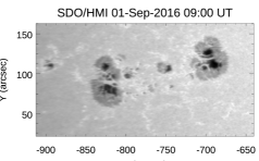
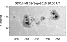
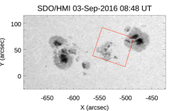
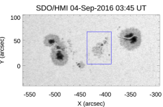
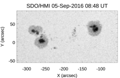
Figure 1: Maps of the continuum intensity of AR NOAA 12585 acquired by SDO/HMI. The red and blue boxes indicate the SST/CRISP and Hinode/SP FOVs analyzed in this study, respectively.

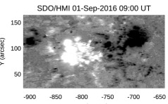
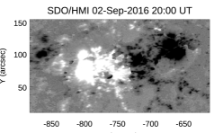
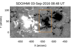
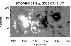
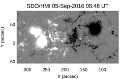
Figure 2: Maps of the LOS magnetograms of AR NOAA 12585 acquired by SDO/HMI. The orange box indicates the FOV where the magnetic flux evolution shown in Figure 3 has been computed.

3 Results

3.1 Global evolution of AR NOAA 12585

Figures 1 and 2 display the large-scale evolution of the AR from September 1 to 5 in the continuum filtegrams and radial magnetograms as acquired by SDO/HMI. The AR is initially characterized by a $\beta$ magnetic configuration and mainly composed by two complex sunspots (see top panels of Fig. 1). These latter exhibit light bridges (see, e.g., Falco et al., 2016; Felipe et al., 2016 and references therein) during the observing time interval, indicating the onset of their fragmentation. It is worth mentioning that the light bridge of the leading sunspot has polarity opposite than the hosting umbra, as recently observed in umbral filaments (Guglielmino et al., 2017, 2019). On September 5, the leading spot displays a smaller size but a more roundish shape with a regular penumbra, while the trailing polarity after a fragmentation process splits in two regions with several umbral cores embedded in more irregular penumbrae (see bottom panels of Fig. 1).

The central region in between the two main AR polarities appears as composed by smaller and more fragmented magnetic structures (see the magnetograms of Fig. 2) showing the formation of two not fully developed sunspots. As a consequence, the magnetic configuration of the AR changes from $\beta$ to $\beta\gamma$ on September 3. From September 1 to 3, this portion of the AR evolves in several pores, forming through the reorganization of the emerged flux by the combined effect of velocity and magnetic field (see Ermolli et al., 2017), and a more extended penumbra. Interestingly, this penumbra forms only eastwards, i.e., towards the opposite polarity, while no penumbra forms on the other side. This sub-system starts to decay before it was able to form a complete penumbra.

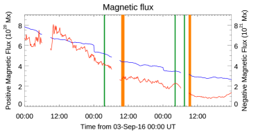
Figure 3: Evolution of positive (red) and negative (blue, absolute value) magnetic flux in the ROI (marked with the orange box in Fig. 2) as derived from SDO/HMI measurements. The orange stripes represent the time of SST/CRISP observations, while the green ones those of the Hinode/SP scans.

3.2 Study of the decay phase of the central region

We computed the variation of the positive and negative magnetic flux (from SDO/HMI) in the subFOV indicated by the orange box in Fig. 2 (bottom-left panel), from September 3 and 5. The plot reported in Fig. 3 clearly shows the decay phase of the central part of the AR. Figure 3 also displays the time intervals covered by the SST/CRISP and Hinode datasets, indicated with the orange and green stripes, respectively. To estimate the decay rate we calculated $d\Phi/dt$, where $\Phi$ represents the total flux corresponding to the sum of the positive and negative (in absolute value) fluxes during the entire time interval. From September 3 to 5, the flux in this region decayed with an average rate of $2\times 10^{16}\,\mathrm{Mx\,s}^{-1}$.
Figure 4 displays the reconstructed continuum intensity (panels a1, b1 and c1), the LP (panels a2, b2 and c2), CP (panels a3, b3 and c3), and LOS velocity (panels a4, b4 and c4) maps derived from the measurements taken by Hinode/SP, respectively at three time steps on September 4 and 5.
The high spatial resolution of the Hinode observations compared to that from SDO, allows seeing, on September 4, the fine structure of the penumbra and its discontinuities: e.g., penumbral grains and patchy bright features are visible at X,Y=[20″,20″] or [15″,30″]. These areas, which are characterized by a higher continuuum intensity, could be interpreted as the manifestation of the intrusion of granulation among the penumbral filaments. Furthermore, these areas display the lowest value of LP signal. Besides, the CP map at 03:45 UT displays positive and negative patches inside the filamentary penumbral structure of the field, resembling MMFs.
Comparing the Hinode/SP maps at different times, we see that the LP maps show a decrease of the horizontal field with time. Moreover, the CP signal that outlines the fine structure of the penumbra becomes weaker as penumbral filaments disappear. The granulation seems fuzzy where the field starts to dissipate and the penumbra dissolves (see the red arrow in panel b1 of Fig. 4). In these regions, the field appears to be mainly horizontal on September 5 at 04:15 and 07:27 UT (see the panels a2, b2 and c2 of Fig. 4), while the continuum intensity maps show the re-organization of the granulation in the southern side of the ROI (see the panel b1 of Fig. 4).

The LOS velocity maps display that the penumbral region is initially redshifted according to the expected classical Evershed flow pattern (see panel a4 of Fig. 4), being located towards the eastern limb. The Evershed flow is visible as long as some penumbral filaments remain (see the ovals in the panels b4 and c4 of Fig. 4). The granulation velocity pattern in the velocity maps takes more time to re-appear in comparison with the disappearance of the penumbra in the continuum intensity maps. In particular, although the filaments are no longer visible in the continuum, the field is still horizontal and the Evershed flow has not completely vanished (see the area delimited by black arrows in continuum intensity, LP, and LOS velocity maps of Fig. 4). However, at the location of some of the disappearing filaments, blue-shifted patches are detected (see the square in the panels b of Fig. 4). These could be attributed to blue shifts due to the 5-min oscillations, which cannot be removed in this Hinode dataset consisting of frames at three times only. Alternatively, they might be related to the remnant of the upflows in the inner penumbra reported by Rimmele (1995), provided that they seem to be linked to the horizontal magnetic field. Nevertheless, we cannot rule out that they could be interpreted as counter-Evershed flows (see Murabito et al., 2016; Siu-Tapia et al., 2017, 2018).

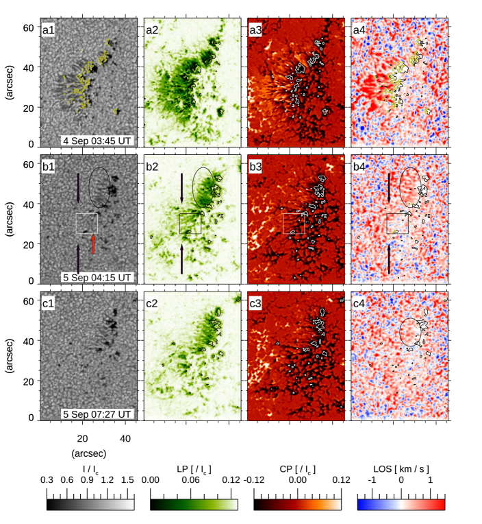
Figure 4: From left to right: Continuum intensity, linear polarization LP, circular polarization CP and LOS velocity relevant to the data acquired during the three Hinode/SP raster scans. The subFOV is the same as the blue box shown in Fig. 1. The black/white contours represent the edge of the umbra ($I_{c}=0.6$) as seen in the continuum intensity. The light green contour in the first continuum and LOS velocity maps indicates contour at $0.1$ $LP/I_{c}$. Arrows, ovals and boxes point to regions and features described in Sect- 3.2.

The CRISP instrument acquired data of the central part of the AR (i.e., similar to that shown in Fig. 4) for more than one hour on September 4. Figure 5 displays maps of continuum intensity (panels a1 and b1), magnetic field strength (panels a2 and b2), inclination angle (panels a3 and b3) and LOS velocity (panels a4 and b4) derived from CRISP data relevant to the observations acquired at 09:31 and 10:37 UT, respectively.

These data, which are characterized by a even higher spatial resolution than the ones from Hinode/SP, allow us to study in more detail the penumbral grains and the patchy bright features, in the inner part of the penumbra around the edge of the southern umbrae (see panels a1 and b1 of Fig. 5). These penumbral grains, also visible in the Hinode/SP data, exhibit both inward and outward motions. The magnetic field strength inside the small umbral cores is stronger than 1.2 kG and it does not show any appreciable changes after one hour, while the field decreases inside the penumbra (identified by the area between $I_{c}=0.7$ and $I_{c}=0.9$) reaching an average value of 0.8 kG (compare panels b1 and b2 of Fig. 5).

The inclination maps show very well the fine structure of the penumbra, with inclination ranging between $80^{\circ}$ and $120^{\circ}$. A ring of patches with a field inclination of $20^{\circ}-30^{\circ}$ encircles the northern side of the penumbra (see panel a3 of Fig. 5, white arrows). These opposite polarity (respect with the small umbral cores) patches correspond to localized bright points in the continuum intensity map, as indicated by the red arrows in panel a1 of Fig. 5). The limited FOV of the CRISP instrument does not allow us to say if other patches are present along the south-eastern side of the penumbra as well. The LOS velocity map at 09:31 UT (panel a4 of Fig. 5) shows the classical Evershed flow pattern inside the whole penumbra, with velocity values on average around $0.5\,\mathrm{km\,s}^{-1}$ and maximum values around $2.7\,\mathrm{km\,s}^{-1}$. One hour later, a few filaments in the northern part of the penumbra start to disappear. Nevertheless, the Evershed flow pattern remains while penumbral filaments disappear (compare the regions indicated by the black arrows in panels b1 and b4 of Fig. 5).

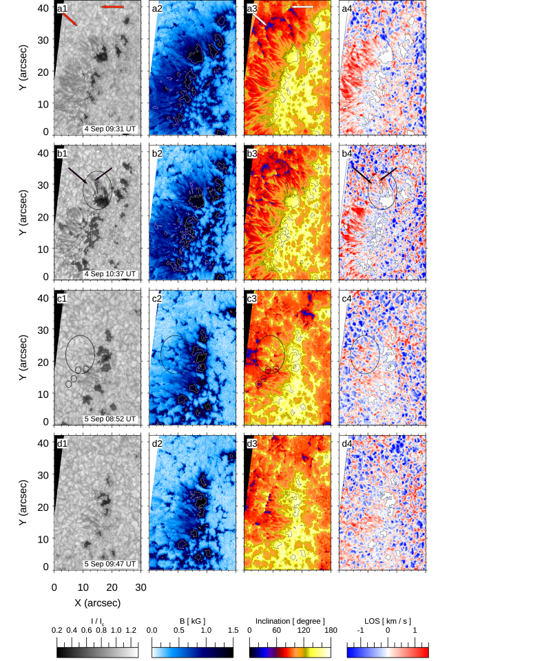
Figure 5: From left to right: Continuum intensity, magnetic field strength, magnetic field inclination, and LOS velocity maps from SST/CRISP observations at four representative times on September 4 and 5. Arrows and ovals mark features described in Sect. 3.2.

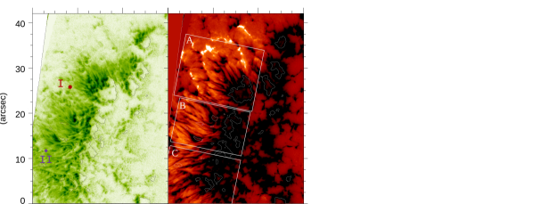
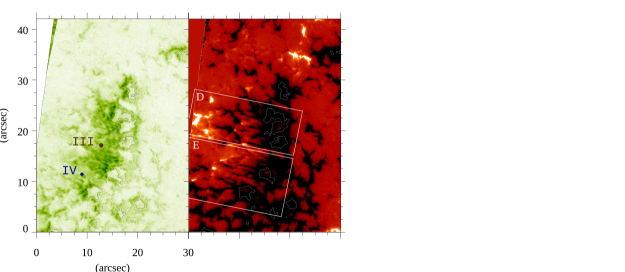
Figure 6: LP and CP maps from SST/CRISP data at 09:31 UT (top panels) and 08:52 UT (bottom panels) on September 4 and 5, respectively. The boxes drawn on the CP maps indicate where the magnetic flux evolution shown in Fig. 8 has been computed. The LP and CP maps are scaled to $0.05\,LP/I_{c}$ and $\pm 0.05\,CP/I_{c}$, respectively. The coloured symbols (I-IV) in LP panels refer to locations considered in Fig. 10. See Sect. 3.2 for more details.

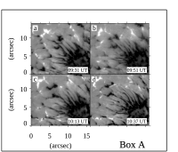
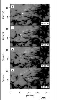
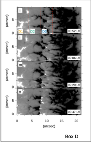
Figure 7: Zoomed CP maps of the box A (panels a-d), E (panels e-h) and D (panels i-n) from the SST/CRISP data at four representative times on September 4 and  5. The boxes are indicated in Fig. 6. All the CP maps are scaled to $\pm 0.05$ $CP/I_{c}$. The three red dashed lines in the first panel relevant to Box D indicate the three regions where the magnetic flux evolution reported in Fig. 9 has been computed.

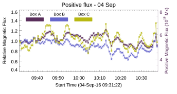
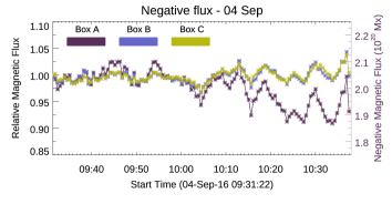
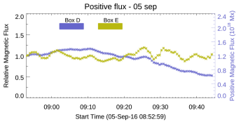
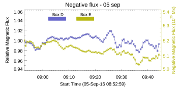
Figure 8: Evolution of the positive (left panels) and negative (right panels) magnetic flux inside the three boxes marked on the CP maps of Fig. 6 computed from the VFISV inversions of the SST/CRISP data on September 4 (top panels) and 5 (bottom panels). Symbols with different colours refer to the various analyzed boxes as specified in the legend.

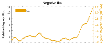
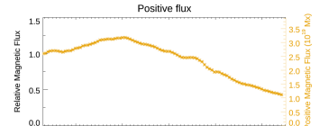
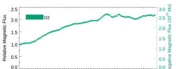
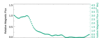
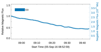
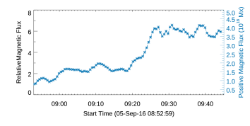
Figure 9: Evolution of the positive (left panels) and negative (right panels) magnetic flux inside the three regions D1, D2 and D3 marked on the CP map of Fig. 6 on September 5. Symbols with different colours refer to the various analyzed boxes as specified in the legend.

On September 5 (panels c and d of Fig. 5) only few penumbral filaments are visible in the southern part of the system. In the first temporal frame, at 08:52 UT, the area located at the northern part of the remaining penumbral sector displays elongated and stretched granules (see the area indicated by the ovals in panels c of Fig. 5). Panels c2 and c3 of Fig. 5 reveal a magnetic field with a sea-serpent-like configuration (Sainz Dalda & Bellot Rubio, 2008). We clearly see large patches of opposite polarity, for instance at X,Y=[5″,20″] and [25″,35″]. Moreover, at the edge of the penumbral filaments in the inclination map there are patches of opposite polarity with respect to the umbral field (see the small ovals in panel c1 and c3 of Fig. 5). In less than one hour, at 09:47 UT (panels d of Fig. 5), the remaining penumbral filaments become thinner and the large-scale opposite polarity patches at the edge of them shrink. Conversely, the structure inside the oval is characterized by coexisting opposite polarity features (see panels c2 and c3 of Fig. 5). This will be further investigated in the following (see Fig. 7).
In order to investigate the dynamics of the fine penumbral structures involved in the penumbral decay, we benefitted from polarization maps derived from CRISP measurements, shown in Fig. 6. In the analyzed region on September 4 horizontal magnetic fields and a large number of MMFs are detected in the time series of CP and LP maps. In particular, the movie available in the online material, relevant to LP map from September 4 data (top-left panel of Fig. 6), displays that the area of the LP signal cospatial to the region where the penumbral filaments are disappearing (near the red filled circle) shrinks along time, although it does not completely vanishes.
The zoomed panels (a-d) of Fig. 7, corresponding to the box A in the CP map from September 4 data (top-right panel of Fig. 6), show the interaction between the penumbral field and opposite polarity patches that could lead to cancel out part of the penumbra. In order to study this aspect, we examined the longitudinal magnetic flux evolution as retrieved from the VFISV inversions of the whole SST/CRISP data. The plots reported in the top panels of Fig. 8 present the relative positive (left panel) and negative (right panel) magnetic flux inside the three boxes drawn over the CP map of the top panels of Fig. 6. It is evident that the negative magnetic flux decreases by about $0.2\times 10^{20}$ Mx inside the box A only (dark violet curve, right panel), where the penumbral filaments disappear. Conversely, the bluish (box B) and yellowish (box C) curves remained almost constant with time. On the whole, the plot reported in the left panel of Fig. 8 reveals that a significant positive magnetic flux inside the box A remains almost constant, about $5.5\times 10^{18}$ Mx, twice as large as the average flux content in box B ($2.0\times 10^{18}$ Mx) and C ($2.3\times 10^{18}$ Mx). This result is in line with the the idea that part of the penumbral field, characterized by a negative polarity, is canceled out by the interaction with the positive polarity patches seen in the CP movie also available in the online material. Concerning the southern part of the region, the CP movie shows that there is no significant concentration of opposite polarity patches interacting with the penumbral field. Indeed, as already anticipated, in box B and box C there is no decrease of the negative magnetic flux producing the disappearance of the penumbra, even if the positive flux remains almost constant.
We used a similar approach to highlight how the penumbral decay process proceeds on September 5 (see bottom panels of Fig. 6). First, from the CP map, we note that the elongated granules, located at the northern part of the remaining penumbral sector and characterized by blueshifted elongated patches in the LOS velocity maps (see the panels c1 and c4 of Fig. 5), are exactly at the right edge of the sea-serpent-like configuration of the field (see the CP map in the bottom-right panel of Fig. 6), which is also visible in the inclination maps (panels c3 and d3 of Fig. 5). Although the penumbra has almost disappeared, LP signal is still detected around the small umbral cores where the filaments disappeared and elongated granules appear (see LP map in the bottom-left panel of Fig. 6). The box E is the only area where some penumbral filaments are still present, while decreasing in size with time. The zoomed panels (e-h) of Fig. 7 illustrate the evolution of this area within the one hour of SST/CRISP observations. As reported for September 4, numerous MMFs can be detected. The bottom panels of Fig. 8 contain the plots for the positive/negative magnetic flux evolution inside the two boxes D and E marked over the CP map in bottom-right panel of Fig. 6. According to this figure, the negative magnetic flux (right panel) in both boxes shows a decrease even if with different trends. Instead, the positive fluxes (left panel) have a different behavior. In fact, while in the box E the positive flux remains constant with time (yellowish curves), this is not the case for the box D (bluish curves). These results are consistent with the idea of the interaction between type III MMFs and the penumbral field.
To disentangle the various magnetic contributions occurring inside the Box D, we also studied the evolution of the positive (negative) flux variation inside three regions marked in panel (i) of Fig. 7. In particular, we considered the D1 region between X=0″and X=4″, the D2 region from X=4″to X=8″and the D3 region between X=8″and X=12″. Figure 9 displays the variation of the magnetic flux inside these three regions. The plots concerning the region D1 (first row of Fig. 9) show a decrease of positive magnetic flux and an increase of the negative one. It is worth noting that the positive flux could decrease because the positive polarity patches seen in this region were not longer included in the FOV. However, these changes in the evolution of the magnetic flux do not have relation with the penumbra and its disappearance. The other two regions (D2 and D3) include the area where the small-scale sea-serpent magnetic configuration is forming at about $2\arcsec-3\arcsec$ away along the prolongation of the penumbral filaments. A constant increase of the negative magnetic flux is detected for the area inside D2, while this region exhibits a decrease of the positive magnetic flux, although with different trends (see second row in Fig. 9). An opposite behaviour is found for the region D3. Indeed, a constant decrease of the negative magnetic flux is associated with a positive magnetic flux increase, even with different rates (see third row in Fig. 9). In particular, the emergence of the positive magnetic flux seen in this latter plot, due to an emerging region moving toward the negative polarity, cancels part of the pre-existing negative polarity flux. Unfortunately, we do not have data acquiring the evolution of this particular structure. However, in the zoomed panels (i-n) of Fig. 7, we observe the separation of type III MMFs that converge towards opposite polarity patches, forming in about one hour the complex, well-outlined structure like a magnetic wall, in line with the evolution of the flux reported above.

In Fig. 10 we present examples of the observed Stokes profiles in the pixels corresponding to the coloured symbols (I-IV) drawn on the LP maps of Fig. 6. The initial time is represented with a darker colour, while the ending time with a lighter colour. The red and blue symbols (I and II) on the LP map on September 4, are located inside the boxes A and C, respectively. In the case of the red symbol (i.e., position marked with I), we note that the Stokes $V$ signal slightly decreases with time while the penumbral filaments disappear in that location (see panel b1 of Fig. 5). At the same time, the Stokes $Q$ and $U$ profiles do not show significant variations. Conversely, the location labelled with the violet diamond symbol (i.e., position marked with II) displays the almost unchanged Stokes $Q$, $U$ and $V$ profiles. Similarly, the brown and blue coloured symbols (i.e., positions labelled with III and IV, respectively) identify special positions, both inside the box C, on 5 September (see the LP map on the bottom-left panel of Fig. 6). The main difference is that one of these pixel positions (the brown one) is located in the area where the penumbra is disappearing and where a large number of MMFs are seen. In this particular case the most important signature results in the decrease of the Stokes $V$ profiles, while the Stokes $Q$ and $U$ profiles do not display considerable changes. On the other hand, the blue symbol, which resides in a “quiet” area, display all the Stokes profiles unchanged, meaning that probably no opposite (positive) polarity patches interact.

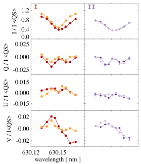
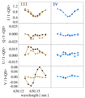
Figure 10: Stokes profiles observed in the pixels (I-IV) marked with coloured filled symbols in the LP maps of Fig. 6 from SST/CRISP observations on September 4 and 5. From top to bottom, we show the four I, Q, U and V Stokes profiles. The colours indicate initial (dark colours symbols) and final (light colours symbols) times of the observations.

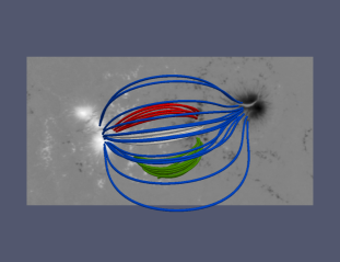
Figure 11: Potential field extrapolation obtained using SDO/HMI LOS magntogram taken on September 3 at 08:48 UT as boundary condition.

4 Discussion and Conclusion

Multi-instrument photospheric observations have allowed us to investigate the decay process of a penumbra in the central part of the AR NOAA 12585.

Thanks to the synoptic SDO/HMI observations, we have been able to follow the entire evolution of this AR from its appearance on the East solar limb on 2016 September 1 till the disappearance of the penumbral areas in its central part. During its evolution (from September 1 to 3), the AR first exhibits a $\beta$ magnetic configuration that changes with time becoming more complex and showing the formation of magnetic structures between the two main polarities. During this time interval, two not fully developed sunspots form in the central region. In this context, we remark a noteworthy aspect about the formation of the penumbra of these two structures: i.e., for both the structures, the penumbra forms only in the region towards the opposite polarity, whereas the area toward the leading spot does not show any penumbral sector. This finding, i.e. the penumbrae do not occur between nearby spots of the same polarity, was already noted by Künzel (1969).

The formation of a penumbra towards the opposite polarity in a flux emergence region occurs in apparent contrast with the observations of Schlichenmaier et al. (2010, 2012) and Rezaei et al. (2012). They found that during the penumbra formation process, penumbral filaments initially do not form in the side facing to the opposite polarity, where the ongoing emerging flux does not allow a stable penumbra to form. However, Murabito et al. (2017) found that the penumbra forms also on the side toward the opposite polarity, i.e. the flux emergence region. Even considering the photospheric evolution of bipolar ARs with the simplest magnetic configuration, i.e. $\beta$ type, a preferred penumbral formation side was not found so far (Murabito et al., 2018). On the other hand, this interpretation assumes that the penumbra formation is mainly linked to the emergence of the magnetic flux from the convection zone. Taking into account the scenario proposed by Romano et al. (2013, 2014, 2020), the penumbra settlement takes place after the magnetic flux emergence, when the magnetic canopy, already present in the upper layers of the solar atmosphere, changes the inclination of its magnetic field, reaching the photosphere and forming the penumbra. In this case, the preferred penumbral formation side does not depend on the location of the emerging magnetic bipole, but on the overlying magnetic field configuration and the magnetic connectivity. In this light, we performed a potential field extrapolation using the SDO/HMI LOS magnetogram taken on September 3 at 08:48 UT as boundary condition (see Fig. 11). The potential field shows the connectivities of the central part of the AR with some positive and diffused polarities located eastwards (see the red, white and green loop systems in Fig. 11). No positive polarities are visible near the leading polarity, therefore no field lines fill the region between the negative polarities of the central part of the AR and the main negative spot. The magnetic field configuration derived from our extrapolation of the HMI data suggests that the penumbra may not form without the presence of the overlying magnetic canopy.

With regard to the penumbal decay, we presented high-resolution measurements available on September 4 and 5 outlining the properties of vector magnetic field and LOS velocity during the disappearance of the different penumbral sectors in the central region of the AR. At that time, the penumbra looked like an orphan penumbra (Zirin & Wang, 1991; Jurčák et al., 2014; Zuccarello et al., 2014).

Although these high-resolution observations only cover a few short time intervals of the processes at work, we have found a number of remarkable and coherent aspects that could help in the understanding of the complex and poorly studied process of penumbral decay.

The main results of our study can be summarized as follow:

1. The negative magnetic flux of the central region decreases from September 3 to 5 with an average rate of $2\times 10^{16}\,\mathrm{Mx\,s}^{-1}$ (corresponding to $1.7\times 10^{21}\,\mathrm{Mx\,day}^{-1}$), till the penumbra completely disappears and only some pores survive.

2. Before the penumbra disappears, opposite polarity patches in the inclination maps are visible. These patches are associated with penumbral bright points in the continuum intensity.

3. Once the penumbral filaments disappear in the continuum intensity, the Evershed flow does not immediately cease to be, but it is only reduced. Furthermore, the area involved by the Evershed flow displays strong LP signals indicating that the field is not completely vertical. As a consequence, after the penumbra disappears, it is not immediately replaced by the granulation and the convective velocity field pattern.

4. The presence of MMFs, progressively located near the sectors which starts to disappear, as well as the magnetic flux evolution suggest that the penumbral magnetic flux may be removed by these features. Furthermore, the analysis of the Stokes profiles where the penumbra is disappearing displays a decrease of the Stokes $V$ profiles and unchanged Stokes $U$ and $Q$ profiles. This is in line with the idea of the flux removal due to the interaction between the negative penumbral field and opposite polarity features, as detected.

5. A small sea-serpent-like magnetic configuration of the magnetic field results from the detached type III MMFs converging toward opposite polarity patches as the penumbral filaments disappeared.

The reported decay rate ($1.7\times 10^{21}\,\mathrm{Mx\,day}^{-1}$) is one order of magnitude greater than that found by Deng et al. (2007), confirming that decay we have observed is faster in comparison with previous observed cases. However, we cannot neglect that Deng et al. (2007) have reported the decay rate of a regular sunspot with umbra and a complete penumbra, while we consider the decay process of a not fully developed sunspot embedded in a more complex magnetic configuration. On the other hand, the decay process simulated in Rempel (2015) for a naked spot reports a steady decay of about $10^{21}\,\mathrm{Mx\,day}^{-1}$, in good agreement with our observed decay rate. Our decay rate measurements is also in line with that reported in Benko et al. (2018), taking into account the appropriate corrections.

Concerning the large-scale opposite polarity patches, we can surely link them to the penumbra formation. Indeed, Romano et al. (2013, 2014) found that, during the formation process of a sunspot penumbra, opposite polarity patches with respect to the parent umbra move radially outward. They interpreted these results as the displacements of the footpoints of the field lines stretching and returning to the photosphere in order to form the penumbra from the inclined magnetic field. In our case, the opposite polarity patches are found also before the disappearance of the penumbra, around the penumbral filaments and associated with localized bright points. Furthermore, in Murabito et al. (2016) the opposite polarity features found around the umbra before the penumbra forms, migrate outward forming a ring that moves away from the spot with time. They suggested that this ring moves presumably driven by the moat flow. Bright features moving in the outer penumbra were also detected in the G-band during the decay of sunspots by Kubo et al. (2008). Their interpretation supports the idea that subsurface upwelling and diverging flows can destabilize the spot, linking MMFs and convective motions. In this perspective, further work should be done to better investigate this aspect and disentangle whether an analogous process happens during the disappearance stage of the penumbra or this signature suggests a role of convection motions in eroding the footpoints of sunspot.

The relationship between the presence of Evershed flow and sunspot decay was studied by Bellot Rubio et al. (2008), who suggested that the penumbra at photospheric level disappears when the penumbral field lines that no longer carry strong Evershed flows rise to the chromosphere. Our results display that the Evershed flow and horizontal fields do not completely vanish after the disappearance of penumbral filaments in the continuum. Therefore, we argue that the Evershed flow persists as long as the horizontal magnetic field lies in the photosphere, although the strength of the magnetic field is not able to keep the reduced heating transport typical of the sunspot penumbra. In addition, blue shifted patches have been detected at the location where penumbral filaments are disappearing. These might be the first indication of reappearance of granulation, or they can be the related to the remnant of the upflows in the inner penumbra (Rimmele, 1995) linked to the horizontal fields. We do not rule out that these blue-shifted patches might be related to counter-Evershed flows,as in turn observed by Murabito et al. (2016, 2018) during penumbra formation and by Siu-Tapia et al. (2017, 2018) in a well-developed sunspot penumbrae. At certain locations, it may even reverse, like during penumbra formation, suggesting an inverse process in temporal sense between penumbral formation and decay. Granulation as well as the convective velocity field pattern take a longer time to reappear as the penumbra disappears in the continuum intensity. In broader perspective, from the SST/CRISP observations, it was possible to highlight that the penumbra does not decay as whole, but different penumbral sectors disappear progressively. Indeed, we have caught the disappearance of two sectors of penumbra, one on the north-eastern side and the other one in the south-eastern side of the region. In such a perspective, the magnetic flux evolution, derived from the spectropolarimetric VFISV inversions of the whole SST/CRISP data, has disclosed useful information to explain this aspect. In fact, the negative magnetic flux decreases in the penumbral sector which firstly disappears on September 4 (the northern one, inside the box A) only. This is accompanied by an almost constant positive magnetic flux. Conversely, for the remaining penumbral sectors, there are no significant changes in the penumbral field, although a similar quantity of positive magnetic flux is found. This provides a robust suggestion that the interaction between opposity polarity fields (type III MMFs) and the penumbral field has a key role during the decay process observed in this AR. On the other hand, benefiting from the extrapolation shown in Fig. 11, we can argue that the different observed connectivities (red, white and green field lines in the extrapolation) may play a role in the onset of the penumbral decay, providing a possible explanation about why the penumbra disappears in sectors and not as a whole. Indeed, the different flux systems overlying the penumbra seem to be topologically separated, and this can be linked to the different instant of disconnection of the canopies leading to penumbral disappearance.

The structure where small-scale opposite polarity features coexist, seen in particular on September 5 in the SST/CRISP observations, could be explained with the schematic illustration resulting from the numerical simulations presented by Kitiashvili et al. (2010), where the sea-serpent configuration results as a consequence of solar overturning magnetoconvection in a highly inclined, strong magnetic field. In particular, the inclined magnetic field deforms the penumbral convective cells, the field lines are stretched and dragged down so that touching the surface form magnetic positive and negative polarities patches.

Finally, what role does the overlying canopy play in the decay of penumbra? The simulation work presented by Rempel (2015) suggested how the strength of the mixed polarity field is based on the strength of the canopy field. Hence, this canopy field, being more prominent for spots than for pores, can have different effects on the size and nature of the region. In the present study, it is difficult to identify whether it initially dominates by triggering the onset of the decay in some part of the penumbra over others or it also plays a role by enhancing the mixed polarity fields leading to flux decay as suggested by the simulations.

The present work brings a valuable contribution to understand the penumbral decay process. However, it is clear that we have not been able to disentangle between the three mechanisms proposed to explain the process, although the role of MMFs and overlying canopies seem to have different spheres of action. Future observations by using space- and ground-based coordinated data, such as those from the PHI instrument (Solanki et al., 2015, 2020) on board of the Solar Orbiter mission (Müller et al., 2013, 2020) and that from the existing (SST, GREGOR, and Goode Solar Telescope) and new 4-meter class telescopes (DKIST and EST) will be essential.

References

- Balthasar (1988) Balthasar, H. 1988, A&AS, 72, 473
- Balthasar et al. (2013) Balthasar, H., Beck, C., Gömöry, P., et al. 2013, Central European Astrophysical Bulletin, 37, 435
- Bellot Rubio et al. (2008) Bellot Rubio, L. R., Tritschler, A., & Martínez Pillet, V. 2008, ApJ, 676, 698. doi:10.1086/527366
- Benko et al. (2018) Benko, M., González Manrique, S. J., Balthasar, H., et al. 2018, A&A, 620, A191. doi:10.1051/0004-6361/201834296
- Bobra et al. (2014) Bobra, M. G., Sun, X., Hoeksema, J. T., et al. 2014, Sol. Phys., 289, 3549
- Borrero et al. (2011) Borrero, J. M., Tomczyk, S., Kubo, M., et al. 2011, Sol. Phys., 273, 267
- Collados et al. (2010) Collados, M., Bettonvil, F., Cavaller, L., et al. 2010, Astronomische Nachrichten, 331, 615. doi:10.1002/asna.201011386
- del Toro Iniesta et al. (1994) del Toro Iniesta, J. C., Tarbell, T. D., & Ruiz Cobo, B. 1994, ApJ, 436, 400
- de la Cruz Rodríguez et al. (2015) de la Cruz Rodríguez, J., Löfdahl, M. G., Sütterlin, P., et al. 2015, A&A, 573, A40. doi:10.1051/0004-6361/201424319
- Deng et al. (2007) Deng, N., Choudhary, D. P., Tritschler, A., et al. 2007, ApJ, 671, 1013. doi:10.1086/523102
- Dravins et al. (1981) Dravins, D., Lindegren, L., & Nordlund, A. 1981, A&A, 96, 345
- Ermolli et al. (2017) Ermolli, I., Cristaldi, A., Giorgi, F., et al. 2017, A&A, 600, A102. doi:10.1051/0004-6361/201526144
- Falco et al. (2016) Falco, M., Borrero, J. M., Guglielmino, S. L., et al. 2016, Sol. Phys., 291, 1939. doi:10.1007/s11207-016-0944-8
- Felipe et al. (2016) Felipe, T., Collados, M., Khomenko, E., et al. 2016, A&A, 596, A59. doi:10.1051/0004-6361/201629586
- Georgoulis (2005) Georgoulis, M. K. 2005, ApJ, 629, L69
- Guglielmino et al. (2017) Guglielmino, S. L., Romano, P., & Zuccarello, F. 2017, ApJ, 846, L16. doi:10.3847/2041-8213/aa835c
- Guglielmino et al. (2018) Guglielmino, S. L., Zuccarello, F., Young, P. R., et al. 2018, ApJ, 856, 127. doi:10.3847/1538-4357/aab2a8
- Guglielmino et al. (2019) Guglielmino, S. L., Romano, P., Ruiz Cobo, B., et al. 2019, ApJ, 880, 34. doi:10.3847/1538-4357/ab2635
- Jurčák et al. (2014) Jurčák, J., Bellot Rubio, L. R., & Sobotka, M. 2014, A&A, 564, A91. doi:10.1051/0004-6361/201322340
- Harvey & Harvey (1973) Harvey, K. & Harvey, J. 1973, Sol. Phys., 28, 61. doi:10.1007/BF00152912
- Keil et al. (2010) Keil, S. L., Rimmele, T. R., Wagner, J., et al. 2010, Astronomische Nachrichten, 331, 609. doi:10.1002/asna.201011385
- Kitiashvili et al. (2010) Kitiashvili, I. N., Bellot Rubio, L. R., Kosovichev, A. G., et al. 2010, ApJ, 716, L181. doi:10.1088/2041-8205/716/2/L181
- Kosugi et al. (2007) Kosugi, T., Matsuzaki, K., Sakao, T., et al. 2007, Sol. Phys., 243, 37
- Künzel (1969) Künzel, H. 1969, Astronomische Nachrichten, 291, 265
- Kubo et al. (2003) Kubo, M., Shimizu, T., & Lites, B. W. 2003, ApJ, 595, 465. doi:10.1086/377333
- Kubo et al. (2007) Kubo, M., Ichimoto, K., Shimizu, T., et al. 2007, PASJ, 59, S607. doi:10.1093/pasj/59.sp3.S607
- Kubo et al. (2008) Kubo, M., Ichimoto, K., Shimizu, T., et al. 2008, First Results From Hinode, 397, 79
- Leka & Skumanich (1998) Leka, K. D. & Skumanich, A. 1998, ApJ, 507, 454. doi:10.1086/306297
- Lites et al. (2013) Lites, B. W., Akin, D. L., Card, G., et al. 2013, Sol. Phys., 283, 579. doi:10.1007/s11207-012-0206-3
- Martínez Pillet et al. (2011) Martínez Pillet, V., Del Toro Iniesta, J. C., Álvarez-Herrero, A., et al. 2011, Sol. Phys., 268, 57. doi:10.1007/s11207-010-9644-y
- Müller et al. (2013) Müller, D., Marsden, R. G., St. Cyr, O. C., et al. 2013, Sol. Phys., 285, 25. doi:10.1007/s11207-012-0085-7
- Müller et al. (2020) Müller, D., St. Cyr, O. C., Zouganelis, I., et al. 2020, A&A, 642, A1. doi:10.1051/0004-6361/202038467
- Murabito et al. (2016) Murabito, M., Romano, P., Guglielmino, S. L., et al. 2016, ApJ, 825, 75
- Murabito et al. (2017) Murabito, M., Romano, P., Guglielmino, S. L., et al. 2017, ApJ, 834, 76. doi:10.3847/1538-4357/834/1/76
- Murabito et al. (2018) Murabito, M., Zuccarello, F., Guglielmino, S. L., et al. 2018, ApJ, 855, 58. doi:10.3847/1538-4357/aaac7c
- Murabito et al. (2020) Murabito, M., Shetye, J., Stangalini, M., et al. 2020, A&A, 639, A59. doi:10.1051/0004-6361/202038360
- Ortiz et al. (2020) Ortiz, A., Hansteen, V. H., Nóbrega-Siverio, D., et al. 2020, A&A, 633, A58. doi:10.1051/0004-6361/201936574
- Pesnell et al. (2012) Pesnell, W. D., Thompson, B. J., & Chamberlin, P. C. 2012, Sol. Phys., 275, 3. doi:10.1007/s11207-011-9841-3
- Quintero Noda et al. (2015) Quintero Noda, C., Asensio Ramos, A., Orozco Suárez, D., et al. 2015, A&A, 579, A3
- Quintero Noda et al. (2016) Quintero Noda, C., Shimizu, T., Ruiz Cobo, B., et al. 2016, MNRAS, 460, 1476
- Rast et al. (2021) Rast, M. P., Bello González, N., Bellot Rubio, L., et al. 2021, Sol. Phys., in press
- Rempel (2015) Rempel, M. 2015, ApJ, 814, 125. doi:10.1088/0004-637X/814/2/125
- Rezaei et al. (2012) Rezaei, R., Bello González, N., & Schlichenmaier, R. 2012, A&A, 537, A19. doi:10.1051/0004-6361/201117485
- Rimmele (1995) Rimmele, T. R. 1995, ApJ, 445, 511. doi:10.1086/175716
- Ruiz Cobo & Asensio Ramos (2013) Ruiz Cobo, B., & Asensio Ramos, A. 2013, A&A, 549, L4
- Romano et al. (2013) Romano, P., Frasca, D., Guglielmino, S. L., et al. 2013, ApJL, 771, L3. doi:10.1088/2041-8205/771/1/L3
- Romano et al. (2014) Romano, P., Guglielmino, S. L., Cristaldi, A., et al. 2014, ApJ, 784, 10. doi:10.1088/0004-637X/784/1/10
- Romano et al. (2020) Romano, P., Murabito, M., Guglielmino, S. L., et al. 2020, ApJ, 899, 129. doi:10.3847/1538-4357/aba18b
- Rouppe van der Voort et al. (2017) Rouppe van der Voort, L., De Pontieu, B., Scharmer, G. B., et al. 2017, ApJ, 851, L6. doi:10.3847/2041-8213/aa99dd
- Sainz Dalda & Bellot Rubio (2008) Sainz Dalda, A. & Bellot Rubio, L. R. 2008, A&A, 481, L21. doi:10.1051/0004-6361:20079115
- Scharmer et al. (2003) Scharmer, G. B., Bjelksjo, K., Korhonen, T. K., et al. 2003, Proc. SPIE, 341
- Scharmer et al. (2008) Scharmer, G. B., Narayan, G., Hillberg, T., et al. 2008, ApJ, 689, L69
- Scherrer et al. (2012) Scherrer, P. H., Schou, J., Bush, R. I., et al. 2012, Sol. Phys., 275, 207
- Schlichenmaier et al. (2010) Schlichenmaier, R., Rezaei, R., Bello González, N., et al. 2010, A&A, 512, L1. doi:10.1051/0004-6361/201014112
- Schlichenmaier et al. (2012) Schlichenmaier, R., Rezaei, R., & González, N. B. 2012, 4th Hinode Science Meeting: Unsolved Problems and Recent Insights, 455, 61
- Schlichenmaier et al. (2019) Schlichenmaier, R., Bellot Rubio, L. R., Collados, M., et al. 2019, arXiv:1912.08650
- Shimizu et al. (2012) Shimizu, T., Ichimoto, K., & Suematsu, Y. 2012, ApJ, 747, L18. doi:10.1088/2041-8205/747/2/L18
- Siu-Tapia et al. (2017) Siu-Tapia, A., Lagg, A., Solanki, S. K., et al. 2017, A&A, 607, A36. doi:10.1051/0004-6361/201730647
- Siu-Tapia et al. (2018) Siu-Tapia, A. L., Rempel, M., Lagg, A., et al. 2018, ApJ, 852, 66. doi:10.3847/1538-4357/aaa007
- Solanki et al. (2015) Solanki, S. K., del Toro Iniesta, J. C., Woch, J., et al. 2015, Polarimetry, 305, 108. doi:10.1017/S1743921315004615
- Solanki et al. (2020) Solanki, S. K., del Toro Iniesta, J. C., Woch, J., et al. 2020, A&A, 642, A11. doi:10.1051/0004-6361/201935325
- Tiwari (2017) Tiwari, S. K. 2017, arXiv:1712.07174
- Tsuneta et al. (2008) Tsuneta, S., Ichimoto, K., Katsukawa, Y., et al. 2008, Sol. Phys., 249, 167
- van Noort et al. (2005) van Noort, M., Rouppe van der Voort, L., & Löfdahl, M. G. 2005, Sol. Phys., 228, 191. doi:10.1007/s11207-005-5782-z
- Verma et al. (2018) Verma, M., Denker, C., Balthasar, H., et al. 2018, A&A, 614, A2. doi:10.1051/0004-6361/201731801
- Zirin & Wang (1991) Zirin, H. & Wang, H. 1991, Advances in Space Research, 11, 225. doi:10.1016/0273-1177(91)90382-T
- Zuccarello et al. (2014) Zuccarello, F., Guglielmino, S. L., & Romano, P. 2014, ApJ, 787, 57. doi:10.1088/0004-637X/787/1/57