Neural Supervised Domain Adaptation by Augmenting Pre-trained Models with Random Units

Abstract

Neural Transfer Learning (TL) is becoming ubiquitous in Natural Language Processing (NLP), thanks to its high performance on many tasks, especially in low-resourced scenarios. Notably, TL is widely used for neural domain adaptation to transfer valuable knowledge from high-resource to low-resource domains. In the standard fine-tuning scheme of TL, a model is initially pre-trained on a source domain and subsequently fine-tuned on a target domain and, therefore, source and target domains are trained using the same architecture. In this paper, we show through interpretation methods that such scheme, despite its efficiency, is suffering from a main limitation. Indeed, although capable of adapting to new domains, pre-trained neurons struggle with learning certain patterns that are specific to the target domain. Moreover, we shed light on the hidden negative transfer occurring despite the high relatedness between source and target domains, which may mitigate the final gain brought by transfer learning. To address these problems, we propose to augment the pre-trained model with normalised, weighted and randomly initialised units that foster a better adaptation while maintaining the valuable source knowledge. We show that our approach exhibits significant improvements to the standard fine-tuning scheme for neural domain adaptation from the news domain to the social media domain on four NLP tasks: part-of-speech tagging, chunking, named entity recognition and morphosyntactic tagging.

1 Introduction

NLP aims to produce resources and tools to understand texts coming from standard languages and their linguistic varieties, such as dialects or user-generated-content in social media platforms. This diversity is a challenge for developing high-level tools that are capable of understanding and generating all forms of human languages. Furthermore, in spite of the tremendous empirical results achieved by NLP models based on Neural Networks (NNs), these models are in most cases based on a supervised learning paradigm, i.e. trained from scratch on large amounts of labelled examples. Nevertheless, such training scheme is not fully optimal. Indeed, NLP neural models with high performance often require huge volumes of manually annotated data to produce powerful results and prevent over-fitting. However, manual data annotation is time-consuming. Besides, language changes over years (Eisenstein, 2019). Thus, most languages varieties are under-resourced (Baumann and Pierrehumbert, 2014; Duong, 2017).

Particularly, in spite of the valuable advantage of social media’s content analysis for a variety of applications (e.g. advertisement, health, or security), this large domain is still poor in terms of annotated data. Furthermore, it has been shown that models intended for news fail to work efficiently on Tweets (Owoputi et al., 2013). This is mainly due to the conversational nature of the text, the lack of conventional orthography, the noise, linguistic errors, spelling inconsistencies, informal abbreviations and the idiosyncratic style of these texts (Horsmann, 2018).

One of the best approaches to address this issue is Transfer Learning (TL); an approach that allows handling the problem of the lack of annotated data, whereby relevant knowledge previously learned in a source problem is leveraged to help in solving a new target problem (Pan et al., 2010). In the context of artificial NNs, TL relies on a model learned on a source-task with sufficient data, further adapted to the target-task of interest. TL has been shown to be powerful for NLP and outperforms the standard supervised learning from scratch paradigm, because it takes benefit from the pre-learned knowledge. Particularly, the standard fine-tuning (SFT) scheme of sequential transfer learning has been shown to be efficient for supervised domain adaptation from the source news domain to the target social media domain (Gui et al., 2017; Meftah et al., 2018b, a; März et al., 2019; Zhao et al., 2017; Lin and Lu, 2018).

In this work we first propose a series of analysis to spot the limits of the standard fine-tuning adaptation scheme of sequential transfer learning. We start by taking a step towards identifying and analysing the hidden negative transfer when transferring from the news domain to the social media domain. Negative transfer (Rosenstein et al., 2005; Wang et al., 2019) occurs when the knowledge learnt in the source domain hampers the learning of new knowledge from the target domain. Particularly, when the source and target domains are dissimilar, transfer learning may fail and hurt the performance, leading to a worse performance compared to the standard supervised training from scratch. In this work, we rather perceive the gain brought by the standard fine-tuning scheme compared to random initialisation as a combination of a positive transfer and a hidden negative transfer. We define positive transfer as the percentage of predictions that were wrongly predicted by random initialisation, but using transfer learning changed to the correct ones. The negative transfer represents the percentage of predictions that were tagged correctly by random initialisation, but using transfer learning gives incorrect predictions. Hence, the final gain brought by transfer learning would be the difference between positive and negative transfer. We show that despite the final positive gain brought by transfer learning from the high-resource news domain to the low-resource social media domain, the hidden negative transfer may mitigate the final gain.

Then we perform an interpretive analysis of individual pre-trained neurons behaviours in different settings. We find that some of pretrained neurons are biased by what they have learnt in the source-dataset. For instance, we observe a unit firing on proper nouns (e.g.“George” and “Washington”) before fine-tuning and on words with capitalised first-letter whether the word is a proper noun or not (e.g. “Man” and “Father”) during fine-tuning. Indeed, in news, only proper nouns start with an upper-case letter. Thus the pre-trained units fail to discard this pattern which is not always respected in user-generated-content in social media. As a consequence of this phenomenon, specific patterns to the target-dataset (e.g. “wanna” or “gonna”) are difficult to learn by pre-trained units. This phenomenon is non-desirable, since such specific units are essential, especially for target-specific classes (Zhou et al., 2018b; Lakretz et al., 2019).

Stemming from our analysis, we propose a new method to overcome the above-mentioned drawbacks of the standard fine-tuning scheme of transfer learning. Precisely, we propose a hybrid method that takes benefit from both worlds, random initialisation and transfer learning, without their drawbacks. It consists in augmenting the source-network (set of pre-trained units) with randomly initialised units (that are by design non-biased) and jointly learn them. We call our method PretRand (Pretrained and Random units). PretRand consists of three main ideas:

1. Augmenting the source-network (set of pre-trained units) with a random branch composed of randomly initialised units, and jointly learn them.

2. Normalising the outputs of both branches to balance their different behaviours and thus forcing the network to consider both.

3. Applying learnable attention weights on both branches predictors to let the network learn which of random or pre-trained one is better for every class.

Our experiments on 4 NLP tasks: Part-of-Speech tagging (POS), Chunking (CK), Named Entity Recognition (NER) and Morphosyntactic Tagging (MST) show that PretRand enhances considerably the performance compared to the standard fine-tuning adaptation scheme.

The remainder of this paper is organised as follows. Section 2 presents the background related to our work: transfer learning and interpretation methods for NLP. Section 3 presents the base neural architecture used for sequence labelling in NLP. Section 4 describes our proposed methods to analyse the standard fine-tuning scheme of sequential transfer learning. Section 5 describes our proposed approach PretRand. Section 6 reports the datasets and the experimental setup. Section 7 reports the experimental results of our proposed methods and is divided into two sub-sections: Sub-section 7.1 reports the empirical analysis of the standard fine-tuning scheme, highlighting its drawbacks. Sub-section 7.2 presents the experimental results of our proposed approach PretRand, showing the effectiveness of PretRand on different tasks and datasets and the impact of incorporating contextualised representations. Finally, section 8 wraps up by discussing our findings and future research directions.

2 Background

Since our work involves two research topics: Sequential Transfer Learning (STL) and Interpretation methods, we discuss in the following sub-sections the state-of-the-art of each topic with a positioning of our contributions regarding each one.

2.1 Sequential Transfer Learning

In STL, training is performed in two stages, sequentially: pretraining on the source task, followed by an adaptation on the downstream target tasks (Ruder, 2019). The purpose behind using STL techniques for NLP can be divided into two main research areas, universal representations and domain adaptation.

Universal representations aim to build neural features (e.g. words embeddings and sentence embeddings) that are transferable and beneficial to a wide range of downstream NLP tasks and domains. Indeed, the probabilistic language model proposed by Bengio et al. (2003) was the genesis of what we call words embedding in NLP, while Word2Vec (Mikolov et al., 2013) was its outbreak and a starting point for a surge of works on learning words embeddings: e.g. FastText (Bojanowski et al., 2017) enriches Word2Vec with subword information. Recently, universal representations re-emerged with contextualised representations, handling a major drawback of traditional words embedding. Indeed, these last learn a single context-independent representation for each word thus ignoring words polysemy. Therefore, contextualised words representations aim to learn context-dependent word embeddings, i.e. considering the entire sequence as input to produce each word’s embedding.

While universal representations seek to be propitious for any downstream task, domain adaptation is designed for particular target tasks. Domain adaptation consists in adapting NLP models designed for specific high-resourced source setting(s) (language, language variety, domain, task, etc) to work in a target low-resourced setting(s). It includes two categories. First, unsupervised domain adaptation assumes that labelled examples in the source domain are sufficiently available, but for the target domain, only unlabelled examples are available. Second, in supervised domain adaptation setting, a small number of labelled target examples are assumed to be available.

Pretraining

In the pretraining stage of STL, a crucial key for the success of transfer is the ruling about the pre-trained task and domain. For universal representations, the pre-trained task is expected to encode useful features for a wide number of target tasks and domains. In comparison, for domain adaptation, the pre-trained task is expected to be most suitable for the target task in mind. We classify pretraining methods into four main categories: unsupervised, supervised, multi-task and adversarial pretraining:

• Unsupervised pretraining uses raw unlabelled data for pretraining. Particularly, it has been successfully used in a wide range of seminal works to learn universal representations. Language modelling task has been particularly used thanks to its ability to capture general-purpose features of language. For instance, TagLM (Peters et al., 2017) is a pretrained model based on a bidirectional language model (biLM), also used to generate ELMo (Embeddings from Language Models) representations (Peters et al., 2018). With the recent emergence of the “Transformers” architectures (Vaswani et al., 2017), many works propose pretrained models based on these architectures (Devlin et al., 2019; Yang et al., 2019; Raffel et al., 2019). Unsupervised pretraining has also been used to improve sequence to sequence learning. We can cite the work of Ramachandran et al. (2017) who proposed to improve the performance of an encoder-decoder neural machine translation model by initialising both encoder and decoder parameters with pretrained weights from two language models.

• Supervised pretraining has been particularly used for cross-lingual transfer (e.g. machine translation (Zoph and Knight, 2016)), cross-task transfer from POS tagging to words segmentation task (Yang et al., 2017) and cross-domain transfer for biomedical texts for question answering by Wiese et al. (2017) and for NER by Giorgi and Bader (2018). Cross-domain transfer has also been used to transfer from news to social media texts for POS tagging (Meftah et al., 2017; März et al., 2019) and sentiment analysis (Zhao et al., 2017). Supervised pretraining has been also used effectively for universal representations learning, e.g. neural machine translation (McCann et al., 2017), language inference (Conneau et al., 2017) and discourse relations (Nie et al., 2017).

• Multi-task pretraining has been successfully applied to learn general universal sentence representations by a simultaneous pretraining on a set of supervised and unsupervised tasks (Subramanian et al., 2018; Cer et al., 2018). Subramanian et al. (2018), for instance, proposed to learn universal sentences representations by a joint pretraining on skip-thoughts, machine translation, constituency parsing, and natural language inference. For domain adaptation, we have performed in (Meftah et al., 2020) a multi-task pretraining for supervised domain adaptation from the news domain to the social media domain.

• Adversarial pretraining is particularly used for domain adaptation when some annotated examples from the target domain are available. Adversarial training (Ganin et al., 2016) is used as a pretraining step followed by an adaptation step on the target dataset. Adversarial pretraining demonstrated its effectiveness in several NLP tasks, e.g. cross-lingual sentiment analysis (Chen et al., 2018). Also, it has been used to learn cross-lingual words embeddings (Lample et al., 2018).

Adaptation

During the adaptation stage of STL, one or more layers from the pretrained model are transferred to the downstream task, and one or more randomly initialised layers are added on top of pretrained ones. Three main adaptation schemes are used in sequential transfer learning: Feature Extraction, Fine-Tuning and the recent Residual Adapters.

In a Feature Extraction scheme, the pretrained layers’ weights are frozen during adaptation, while in Fine-Tuning scheme weights are tuned. Accordingly, the former is computationally inexpensive while the last allows better adaptation to target domains peculiarities. In general, fine-tuning pretrained models begets better results, except in cases wherein the target domain’s annotations are sparse or noisy (Dhingra et al., 2017; Mou et al., 2016). Peters et al. (2019) found that for contextualised representations, both adaptation schemes are competitive, but the appropriate adaptation scheme to pick depends on the similarity between the source and target problems. Recently, Residual Adapters were proposed by Houlsby et al. (2019) to adapt pretrained models based on Transformers architecture, aiming to keep Fine-Tuning scheme’s advantages while reducing the number of parameters to update during the adaptation stage. This is achieved by adding adapters (intermediate layers with a small number of parameters) on top of each pretrained layer. Thus, pretrained layers are frozen, and only adapters are updated during training. Therefore, Residual Adapters performance is near to Fine-tuning while being computationally cheaper (Pfeiffer et al., 2020b, a, c).

Our work

Our work falls under supervised domain adaptation research area. Specifically, cross-domain adaptation from the news domain to the social media domain. The fine-tuning adaptation scheme has been successfully applied on domain adaptation from the news domain to the social media domain (e.g. adversarial pretraining (Gui et al., 2017) and supervised pretraining (Meftah et al., 2018a)). In this research, we highlight the aforementioned drawbacks (biased pre-trained units and the hidden negative transfer) of the standard fine-tuning adaptation scheme. Then, we propose a new adaptation scheme (PretRand) to handle these problems. Furthermore, while ELMo contextualised words representations efficiency has been proven for different tasks and datasets (Peters et al., 2019; Fecht et al., 2019; Schumacher and Dredze, 2019), here we investigate their impact when used, simultaneously, with a sequential transfer learning scheme for supervised domain adaptation.

2.2 Interpretation methods for NLP

Recently, a rising interest is devoted to peek inside black-box neural NLP models to interpret their internal representations and their functioning. A variety of methods were proposed in the literature, here we only discuss those that are most related to our research.

Probing tasks is a common approach for NLP models analysis used to investigate which linguistic properties are encoded in the latent representations of the neural model (Shi et al., 2016). Concretely, given a neural model $\mathbf{M}$ trained on a particular NLP task, whether it is unsupervised (e.g. language modelling (LM)) or supervised (e.g. Neural Machine Translation (NMT)), a shallow classifier is trained on top of the frozen $\mathbf{M}$ on a corpus annotated with the linguistic properties of interest. The aim is to examine whether $\mathbf{M}$’s hidden representations encode the property of interest. For instance, Shi et al. (2016) found that different levels of syntactic information are learned by NMT encoder’s layers. Adi et al. (2016) investigated what information (between sentence length, words order and word-content) is captured by different sentence embedding learning methods. Conneau et al. (2018) proposed 10 probing tasks annotated with fine-grained linguistic properties and compared different approaches for sentence embeddings. Zhu et al. (2018) inspected which semantic properties (e.g. negation, synonymy, etc.) are encoded by different sentence embeddings approaches. Furthermore, the emergence of contextualised words representations have triggered a surge of works on probing what these representations are learning (Liu et al., 2019a; Clark et al., 2019). This approach, however, suffers from two main flaws. First, probing tasks examine properties captured by the model at a coarse-grained level, i.e. layers representations, and thereby, will not identify features captured by individual neurons. Second, probing tasks will not identify linguistic properties that do not appear in the annotated probing datasets (Zhou et al., 2018a).

Individual units stimulus: Inspired by works on receptive fields of biological neurons (Hubel and Wiesel, 1965), much work has been devoted for interpreting and visualising individual hidden units stimulus-features in neural networks. Initially, in computer vision (Coates and Ng, 2011; Girshick et al., 2014; Zhou et al., 2015), and more recently in NLP, wherein units activations are visualised in heatmaps. For instance, Karpathy et al. (2016) visualised character-level Long Short-Term Memory (LSTM) cells learned in language modelling and found multiple interpretable units that track long-distance dependencies, such as line lengths and quotes; Radford et al. (2017) visualised a unit which performs sentiment analysis in a language model based on Recurrent Neural Networks (RNNs); Bau et al. (2019) visualised neurons specialised on tense, gender, number, etc. in NMT models; and Kádár et al. (2017) proposed top-k-contexts approach to identify sentences, an thus linguistic patterns, sparking the highest activation values of each unit in an RNNs-based model.

Neural representations correlation analysis: Cross-network and cross-layers correlation is a significant approach to gain insights on how internal representations may vary across networks, network-depth and training time. Suitable approaches are based on Correlation Canonical Analysis (CCA) (Hotelling, 1992; Uurtio et al., 2018), such as Singular Vector Canonical Correlation Analysis (Raghu et al., 2017) and Projected Weighted Canonical Correlation Analysis (Morcos et al., 2018), that were successfully used in NLP neural models analysis. For instance, it was used by Bau et al. (2019) to calculate cross-networks correlation for ranking important neurons in NMT and LM. Saphra and Lopez (2019) applied it to probe the evolution of syntactic, semantic, and topic representations cross-time and cross-layers. Raghu et al. (2019) compared the internal representations of models trained from scratch vs models initialised with pre-trained weights. CCA based methods aim to calculate similarity between neural representations at the coarse-grained level. In contrast, correlation analysis at the fine-grained level, i.e. between individual neurons, has also been explored in the literature. Initially, Li et al. (2015) used Pearson’s correlation to examine to which extent each individual unit is correlated to another unit, either within the same network or between different networks. The same correlation metric was used by Bau et al. (2019) to determine important neurons in NMT and LM tasks.

Our Work:

In this work, we propose two approaches (section 4.2) to highlight the bias effect in the standard fine-tuning scheme of transfer learning in NLP, the first method is based on individual units stimulus and the second on neural representations correlation analysis. To the best of our knowledge, we are the first to harness these interpretation methods to analyse individual units behaviour in a transfer learning scheme. Furthermore, the most analysed tasks in the literature are Natural Language Inference, NMT and LM (Belinkov and Glass, 2019), here we target under-explored tasks in visualisation works such as POS, MST, CK and NER.

3 Base Neural Sequence Labelling Model

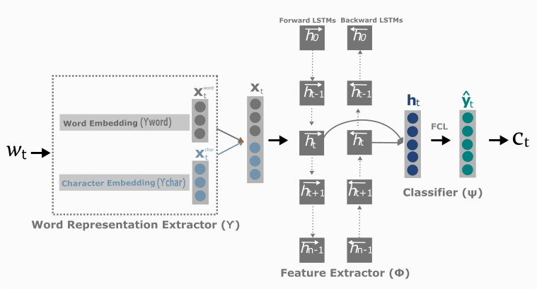
Figure 1: Illustrative scheme of the base neural model for sequence labelling tasks.

Given an input sentence $S$ of $n$ successive tokens $S=[w_{1},\ldots,w_{n}]$, the goal of sequence labelling is to predict the label $c_{t}$ $\in$ $\mathcal{C}$ of every $w_{t}$, with $\mathcal{C}$ being the tag-set. We use a commonly used end-to-end neural sequence labelling model (Ma and Hovy, 2016; Plank et al., 2016; Yang et al., 2018), which is composed of three components (illustrated in Figure 1). First, the Word Representation Extractor ($\mathbf{WRE}$), denoted $\Upsilon$, computes a vector representation $\mathbf{x}_{t}$ for each token $w_{t}$. Second, this representation is fed into a Feature Extractor ($\mathbf{FE}$) based on a bidirectional Long Short-Term Memory (biLSTM) network (Graves et al., 2013), denoted $\Phi$. It produces a hidden representation, $\mathbf{h}_{t}$, that is fed into a Classifier ($\mathbf{Cl}$): a fully-connected layer (FCL), denoted $\Psi$. Formally, given $w_{t}$, the logits are obtained using the following equation: $\hat{\mathbf{y}}_{t}=(\Psi\circ\Phi\circ\Upsilon)(w_{t})$.

In the standard supervised training scheme, the three modules are jointly trained from scratch by minimising the Softmax Cross-Entropy (SCE) loss using the Stochastic Gradient Descent (SGD) algorithm.

Let us consider a training set of $M$ annotated sentences, where each sentence $i$ is composed of $m_{i}$ tokens. Given a training word $(w_{i,t},y_{i,t})$ from the training sentence $i$, where $y_{i,t}$ is the gold standard label for the word $w_{i,t}$, the cross-entropy loss for this example is calculated as follows:

$$\mathcal{L}^{(i,t)}~{}=~{}-~{}y_{i,t}~{}\times~{}log(\hat{y}_{i,t})~{}.$$ (1)

Thus, during the training of the sequence labelling model on $M$ annotated sentences, the model’s loss is defined as follows:

$$\mathcal{L}~{}=~{}\sum_{i=1}^{M}~{}\sum_{t=1}^{m_{i}}~{}\mathcal{L}^{(i,t)}~{}.$$ (2)

4 Analysis of the Standard Fine-Tuning Scheme

The standard fine-tuning scheme consists in transferring a part of the learned weights from a source model to initialise the target model, which is further fine-tuned on the target task with a small number of training examples from the target domain. Given a source neural network $\mathcal{M}_{s}$ with a set of parameters $\theta_{s}$ split into two sets: $\theta_{s}=(\theta_{s}^{1},\theta_{s}^{2})$ and a target network $\mathcal{M}_{t}$ with a set of parameters $\theta_{t}$ split into two sets: $\theta_{t}=(\theta_{t}^{1},\theta_{t}^{2})$, the standard fine-tuning scheme of transfer learning includes three simple yet effective steps:

1. We train the source model on annotated data from the source domain on a source dataset.

2. We transfer the first set of parameters from the source network $\mathcal{M}_{s}$ to the target network $\mathcal{M}_{t}$: $\theta_{t}^{1}=\theta_{s}^{1}$, whereas the second set $\theta_{t}^{2}$ of parameters is randomly initialised.

3. Then, the target model is further fine-tuned on the small target data-set.

Source and target datasets may have different tag-sets, even within the same NLP task. Hence, transferring the parameters of the classifier ($\Psi$) may not be feasible in all cases. Therefore, in our experiments, WRE’s layers ($\Upsilon$) and FE’s layers ($\Phi$) are initialised with the source model’s weights and $\Psi$ is randomly initialised. Then, the three modules are further jointly trained on the target-dataset by minimising a SCE loss using the SGD algorithm.

4.1 The Hidden Negative Transfer

It has been shown in many works in the literature (Rosenstein et al., 2005; Ge et al., 2014; Ruder, 2019; Gui et al., 2018; Cao et al., 2018; Chen et al., 2019; Wang et al., 2019; O’Neill, 2019) that, when the source and target domains are less related (e.g. languages from different families), sequential transfer learning may lead to a negative effect on the performance, instead of improving it. This phenomenon is referred to as negative transfer. Precisely, negative transfer is considered when transfer learning is harmful to the target task/dataset, i.e. the performance when using transfer learning algorithm is lower than that with a solely supervised training on in-target data (Torrey and Shavlik, 2010).

In NLP, negative transfer phenomenon has only seldom been studied. We can cite the recent work of Kocmi (2020) who evaluated the negative transfer in transfer learning in neural machine translation when the transfer is performed between different language-pairs. They found that: 1) The distributions mismatch between source and target language-pairs does not beget a negative transfer. 2) The transfer may have a negative impact when the source language-pair is less-resourced compared to the target one, in terms of annotated examples.

Our experiments in (Meftah et al., 2018a, b) have shown that transfer learning techniques from the news domain to the social media domain using the standard fine-tuning scheme boosts the tagging performance. Hence, following the above definition, transfer learning from news to social media does not beget a negative transfer. Contrariwise, in this work, we instead consider the hidden negative transfer, i.e. the percentage of predictions that were correctly tagged by random initialisation, but using transfer learning gives wrong predictions.

Let us consider the gain $\mathcal{G}_{i}$ brought by the standard fine-tuning scheme (SFT) of transfer learning compared to the random initialisation for a dataset ${i}$. $\mathcal{G}_{i}$ is defined as the difference between positive transfer $\mathcal{PT}_{i}$ and negative transfer $\mathcal{NT}_{i}$:

$$\mathcal{G}_{i}=\mathcal{PT}_{i}-\mathcal{NT}_{i},$$ (3)

where positive transfer $\mathcal{PT}_{i}$ represents the percentage of tokens that were wrongly predicted by random initialisation, but the SFT changed to the correct ones. Negative transfer $\mathcal{NT}_{i}$ represents the percentage of words that were tagged correctly by random initialisation, but using SFT gives wrong predictions. $\mathcal{PT}_{i}$ and $\mathcal{NT}_{i}$ are defined as follows:

$$\mathcal{PT}_{i}=\frac{N^{corrected}_{i}}{N_{i}},$$ (4)

$$\mathcal{NT}_{i}=\frac{N^{falsified}_{i}}{N_{i}},$$ (5)

where $N_{i}$ is the total number of tokens in the validation-set, $N^{corrected}_{i}$ is the number of tokens from the validation-set that were wrongly tagged by the model trained from scratch but are correctly predicted by the SFT scheme, and $N^{falsified}_{i}$ is the number of tokens from the validation-set that were correctly tagged by the model trained from scratch but are wrongly predicted by the SFT scheme.

4.2 Interpretation of Pretrained Neurons

Here, we propose to perform a set of analysis techniques to gain some insights into how the inner pretrained representations are updated during fine-tuning on social media datasets when using the standard fine-tuning scheme of transfer learning. For this, we propose to analyse the feature extractor’s ($\Phi$) activations. Precisely, we attempt to visualise biased neurons, i.e. pre-trained neurons that do not change that much from their initial state.

Let us consider a validation-set of $N$ words, the feature extractor $\Phi$ generates a matrix ${\mathbf{h}}~{}\in~{}{\mathbf{M}_{N,H}(\mathbb{R})}$ of activations over all the words of the validation-set, where $\mathbf{\mathbf{M}_{f,g}(\mathbb{R})}$ is the space of $f~{}\times~{}g$ matrices over $\mathbb{R}$ and $H$ is the size of the hidden representation (number of neurons). Each element $h_{i,j}$ from the matrix represents the activation of the neuron $j$ on the word $w_{i}$.

Given two models, the first before fine-tuning and the second after fine-tuning, we obtain two matrices $\mathbf{h}^{before}~{}\in~{}{\mathbf{M}_{N,H}(\mathbb{R})}$ and $\mathbf{h}^{after}~{}\in~{}{\mathbf{M}_{N,H}(\mathbb{R})}$, which give the activations of $\Phi$ over all validation-set’s words before and after fine-tuning, respectively.

We aim to visualise and quantify the change of the representations generated by the model from the initial state, $\mathbf{h}^{before}$ (before fine-tuning), to the final state, $\mathbf{h}^{after}$ (after fine-tuning). For this purpose, we perform two experiments:

1. Quantifying the change of pretrained individual neurons (section 4.2.1);

2. Visualising the evolution of pretrained neurons stimulus during fine-tuning (section 4.2.2).

4.2.1 Quantifying the change of individual pretrained neurons

In order to quantify the change of the knowledge encoded in pretrained neurons after fine-tuning, we propose to calculate the similarity (correlation) between neurons activations before and after fine-tuning, when using the SFT adaptation scheme. Precisely, we calculate the correlation coefficient between each neuron’s activations on the target-domain validation-set before starting fine-tuning and at the end of fine-tuning.

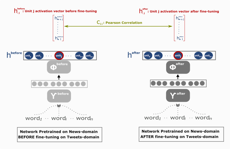
Figure 2: Illustrative scheme of the computation of the charge of unit $j$, i.e. the Pearson correlation between unit $j$ activations vector after fine-tuning to its activations vector before fine-tuning.

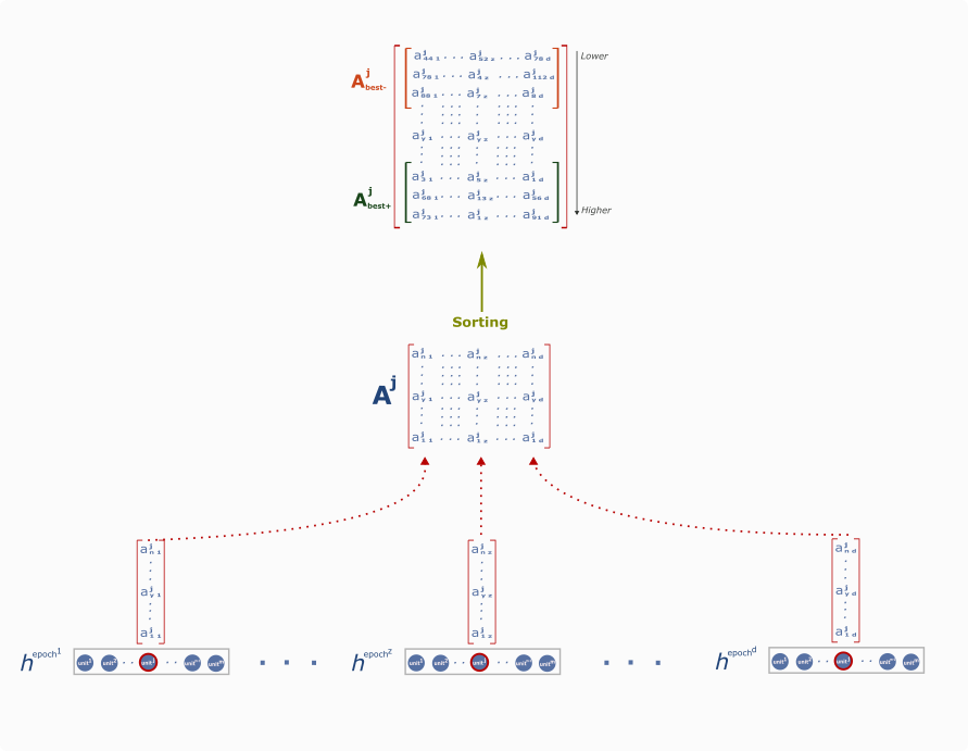
Figure 3: Illustrative scheme of the calculus of top-k-words activating unit $j$, positively ($\mathbf{A}^{(j)}_{best+}$) and negatively ($\mathbf{A}^{(j)}_{best-}$) during fine-tuning epochs. $\mathbf{h}^{epoch^{z}}$ states for $\Phi$’s outputs at epoch number $z$.

Following the above formulation and as illustrated in Figure 2, from $\mathbf{h}^{before}$ and $\mathbf{h}^{after}$ matrices, we extract two vectors $\mathbf{h}^{before}_{.j}~{}\in$ $\mathbb{R}^{N}$ and $\mathbf{h}^{after}_{.j}\in$ $\mathbb{R}^{N}$, representing respectively the activations of a unit $j$ over all validation-set’s words before and after fine-tuning. Next, we generate an asymmetric correlation matrix $\mathbf{C}\in$ ${\mathbf{M}_{H,H}(\mathbb{R})}$, where each element $\mathbf{c}_{jt}$ in the matrix represents the Pearson’s correlation between the activation vector of unit $j$ after fine-tuning ($\mathbf{h}^{after}_{.j}$) and the activation vector of unit $t$ before fine-tuning ($\mathbf{h}^{before}_{.t}$), computed as follows:

$$\mathbf{c}_{jt}=\frac{\mathbb{E}[(\mathbf{h}^{after}_{.j}-\mu^{after}_{j})(\mathbf{h}^{before}_{.t}-\mu^{before}_{t})]}{\sigma^{after}_{j}\sigma^{before}_{t}}~{}.$$ (6)

Here $\mu^{before}_{j}$ and $\sigma^{before}_{j}$ represent, respectively, the mean and the standard deviation of unit $j$ activations over the validation set. Clearly, we are interested by the matrix diagonal, where $c_{jj}$ represents the charge of each unit $j$ from $\Phi$, i.e. the correlation between each unit’s activations after fine-tuning to its activations before fine-tuning.

4.2.2 Visualising the Evolution of Pretrained Neurons Stimulus during Fine-tuning

Here, we perform units visualisation at the individual-level to gain insights on how the patterns encoded by individual units progress during fine-tuning when using the SFT scheme. To do this, we generate top-k activated words by each unit; i.e. words in the validation-set that fire the most the said unit, positively and negatively (since LSTMs generate positive and negative activations). In (Kádár et al., 2017), top-k activated contexts from the model were plotted at the end of training (the best model), which shows on what each unit is specialised, but it does not give insights about how the said unit is evolving and changing during training. Thus, taking into account only the final state of training does not reveal the whole picture. Here, we instead propose to generate and plot top-k words activating each unit throughout the adaptation stage. We follow two main steps (as illustrated in Figure 3):

1. We represent each unit $j$ from $\Phi$ with a random matrix $\mathbf{A}^{(j)}\in$ ${\mathbf{M}_{N,D}(\mathbb{R})}$ of the said unit’s activations on all the validation-set at different training epochs, where $D$ is the number of epochs and $N$ is the number of words in the validation-set. Thus, each element $a^{(j)}_{y,z}$ represents the activation of the unit $j$ on the word $w_{y}$ at the epoch $z$.

2. We carry out a sorting of each column of the matrix (each column represents an epoch) and pick the higher k words (for top-k words firing the unit positively) and the lowest k words (for top-k words firing the unit negatively), leading to two matrices, $\mathbf{A}^{(j)}_{best+}\in$ $\mathbf{\mathbf{M}_{D,k}(\mathbb{R})}$ and $\mathbf{A}^{(j)}_{best-}\in$ $\mathbf{\mathbf{M}_{D,k}(\mathbb{R})}$, the first for top-k words activating positively the unit $j$ at each training epoch, and the last for top-k words activating negatively the unit $j$ at each training epoch.

5 Joint Learning of Pretrained and Random Units: PretRand

We found from our analysis (in section 7.1) on pre-trained neurons behaviours, that the standard fine-tuning scheme suffers from a main limitation. Indeed, some pre-trained neurons still biased by what they have learned from the source domain despite the fine-tuning on target domain. We thus propose a new adaptation scheme, PretRand, to take benefit from both worlds, the pre-learned knowledge in the pretrained neurons and the target-specific features easily learnt by random neurons. PretRand, illustrated in Figure 4, consists of three steps:

1. Augmenting the pre-trained branch with a random one to facilitate the learning of new target-specific patterns (section 5.1);

2. Normalising both branches to balance their behaviours during fine-tuning (section 5.2);

3. Applying learnable weights on both branches to let the network learn which of random or pre-trained one is better for every class. (section 5.3).

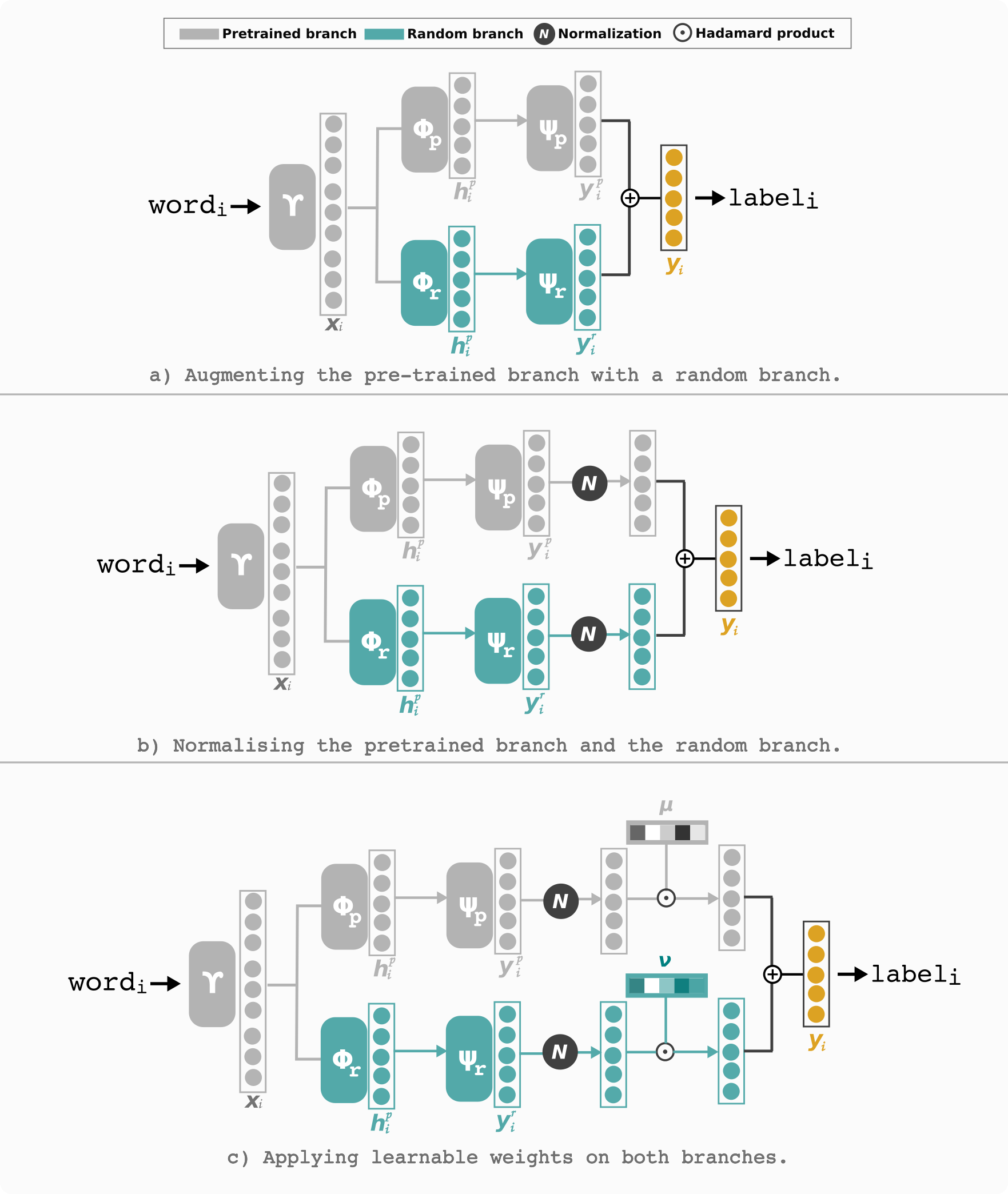
Figure 4: Illustrative scheme of the three ideas composing our proposed adaptation method, PretRand. a) We augment the pre-trained branch (grey branch) with a randomly initialised one (green branch) and jointly adapt them with pre-trained ones (grey branch). An element-wise sum is further applied to merge the two branches. b) Before merging, we balance the different behaviours of pre-trained and random units, using an independent normalisation ($\mathbf{N}$). c) Finally we let the network learn which of pre-trained or random neurons are more suited for every class, by performing an element-wise product of the FC layers with learnable weighting vectors ($\mathbf{u}$ and $\mathbf{v}$ initialised with 1-values).

5.1 Adding the Random Branch

We expect that augmenting the pretrained model with new randomly initialised neurons allows a better adaptation during fine-tuning. Thus, in the adaptation stage, we augment the pre-trained model with a random branch consisting of additional random units (as illustrated in the scheme “a” of Figure 4). Several works have shown that deep (top) layers are more task-specific than shallow (low) ones (Peters et al., 2018; Mou et al., 2016). Thus, deep layers learn generic features easily transferable between tasks. In addition, word embeddings (shallow layers) contain the majority of parameters. Based on these factors, we choose to expand only the top layers as a trade-off between performance and number of parameters (model complexity). In terms of the expanded layers, we add an extra biLSTM layer of $k$ units in the $\mathbf{FE}$ ($\Phi_{r}$ - $r$ for random); and a new fully-connected layer of $C$ units (called $\Psi_{r}$). With this choice, we increase the complexity of the model only $1.02\times$ compared to the base one (The standard fine-tuning scheme).

Concretely, for every $w_{i}$, two predictions vectors are computed; $\hat{\mathbf{y}}_{i}^{p}$ from the pre-trained branch and $\hat{\mathbf{y}}_{i}^{r}$ from the random one. Specifically, the pre-trained branch predicts class-probabilities following:

$$\hat{\mathbf{y}}^{p}_{i}=(\Psi_{p}\circ\Phi_{p})(\mathbf{x}_{i}),$$ (7)

with $\mathbf{x}_{i}=\Upsilon(w_{i})$. Likewise, the additional random branch predicts class-probabilities following:

$$\hat{\mathbf{y}}^{r}_{i}=(\Psi_{r}\circ\Phi_{r})(\mathbf{x}_{i}).$$ (8)

To get the final predictions, we simply apply an element-wise sum between the outputs of the pre-trained branch and the random branch:

$$\hat{\mathbf{y}}_{i}=\hat{\mathbf{y}}_{i}^{p}\oplus\hat{\mathbf{y}}_{i}^{r}.$$ (9)

As in the classical scheme, the SCE loss is minimised but here, both branches are trained jointly.

5.2 Independent Normalisation

Our first implementation of adding the random branch was less effective than expected. The main explanation is that the pre-trained units were dominating the random units, which means that the weights as well as the gradients and outputs of pre-trained units absorb those of the random units. As illustrated in the left plot of Figure 5, the absorption phenomenon stays true even at the end of the training process; we observe that random units weights are closer to zero. This absorption propriety handicaps the random units in firing on the words of the target dataset.

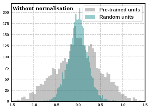
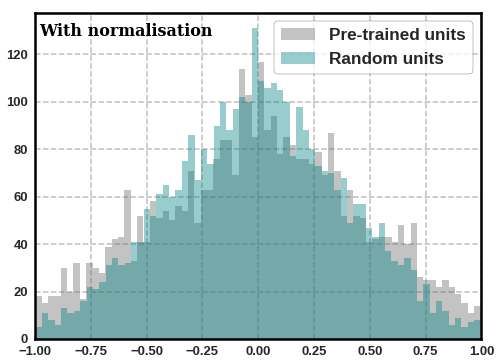
Figure 5: The distributions of the learnt weight-values for the randomly initialised (green) and pre-trained (grey) fully-connected layers after their joint training. Left: without normalisation, right: with normalisation.

To alleviate this absorption phenomenon and push the random units to be more competitive, we normalise the outputs of both branches ($\hat{\mathbf{y}}_{i}^{p}$ and $\hat{\mathbf{y}}_{i}^{r}$) using the $\ell_{2}$-norm, as illustrated in the scheme “b” of Figure 4. The normalisation of a vector “$\mathbf{x}$” is computed using the following formula:

$$\mathbf{N}_{2}(\mathbf{x})=[\frac{\mathbf{x}_{i}}{||\mathbf{x}||_{2}}]_{i=1}^{i=|\mathbf{x}|}.$$ (10)

Thanks to this normalisation, the absorption phenomenon was solved, and the random branch starts to be more effective (see the right distribution of Figure 5).

Furthermore, we have observed that despite the normalisation, the performance of the pre-trained classifiers is still much better than the randomly initialised ones. Thus, to make them more competitive, we propose to start with optimising only the randomly initialised units while freezing the pre-trained ones, then, we launch the joint training. We call this technique random++.

5.3 Attention Learnable Weighting Vectors

Heretofore, pre-trained and random branches participate equally for every class’ predictions, i.e. we do not weight the dimensions of $\hat{\mathbf{y}}_{i}^{p}$ and $\hat{\mathbf{y}}_{i}^{r}$ before merging them with an element-wise summation. Nevertheless, random classifiers may be more efficient for specific classes compared to pre-trained ones and vice-versa. In other terms, we do not know which of the two branches (random or pre-trained) is better for making a suitable decision for each class. For instance, if the random branch is more efficient for predicting a particular class $c_{j}$, it would be better to give more attention to its outputs concerning the class $c_{j}$ compared to the pretrained branch.

Therefore, instead of simply performing an element-wise sum between the random and pre-trained predictions, we first weight $\hat{\mathbf{y}}_{i}^{p}$ with a learnable weighting vector $\mathbf{u}~{}\in~{}\mathbb{R}^{C}$ and $\hat{\mathbf{y}}_{i}^{r}$ with a learnable weighting vector $\mathbf{v}~{}\in~{}\mathbb{R}^{C}$, where $C$ is the tagset size (number of classes). Such as, the element $\mathbf{u}_{j}$ from the vector $\mathbf{u}$ represents the random branch’s attention weight for the class $c_{j}$, and the element $\mathbf{v}_{j}$ from the vector $\mathbf{v}$ represents the pretrained branch’s attention weight for the class $c_{j}$. Then, we compute a Hadamard product with their associated normalised predictions (see the scheme “c” of Figure 4). Both vectors $\mathbf{u}$ and $\mathbf{v}$ are initialised with 1-values and are fine-tuned by back-propagation. Formally, the final predictions are computed as follows:

$$\hat{\mathbf{y}}_{i}=\mathbf{u}~{}\odot~{}\mathbf{N}_{p}(\hat{\mathbf{y}}_{i}^{p})~{}\oplus~{}\mathbf{v}~{}\odot~{}\mathbf{N}_{p}(\hat{\mathbf{y}}_{i}^{r}).$$ (11)

6 Experimental Settings

Task	#Classes	Sources	Eval. Metrics	# Tokens-splits (train - val - test)
POS: POS Tagging	36	WSJ	Top-1 Acc.	912,344 - 131,768 - 129,654
CK: Chunking	22	CONLL-2000	Top-1 Acc.	211,727 - n/a - 47,377
NER: Named Entity Recognition	4	CONLL-2003	Top-1 Exact-match F1.	203,621 - 51,362 - 46,435
MST: Morpho-syntactic Tagging	1304	Slovene-news	Top-1 Acc.	439k - 58k - 88k
	772	Croatian-news	Top-1 Acc.	379k - 50k - 75k
	557	Serbian-news	Top-1 Acc.	59k - 11k, 16k
POS: POS Tagging	40	TPoS	Top-1 Acc.	10,500 - 2,300 - 2,900
	25	ArK	Top-1 Acc.	26,500 - / - 7,700
	17	TweeBank	Top-1 Acc.	24,753 - 11,742 - 19,112
CK: Chunking	18	TChunk	Top-1 Top-1 Acc..	10,652 - 2,242 - 2,291
NER: Named Entity Recognition	6	WNUT-17	Top-1 Exact-match F1.	62,729 - 15,734 - 23,394
MST: Morpho-syntactic Tagging	1102	Slovene-sm	Top-1 Acc.	37,756 - 7,056 - 19,296
	654	Croatian-sm	Top-1 Acc.	45,609 - 8,886 - 21,412
	589	Serbian-sm	Top-1 Acc.	45,708- 9,581- 23,327

Table 1: Statistics of the used datasets. Top: datasets of the source domain. Bottom: datasets of the target domain.

6.1 Datasets

We conduct experiments on supervised domain adaptation from the news domain (formal texts) to the social media domain (noisy texts) for English Part-Of-Speech tagging (POS), Chunking (CK) and Named Entity Recognition (NER). In addition, we experiment on Morpho-syntactic Tagging (MST) of three South-Slavic languages: Slovene, Croatian and Serbian. For POS task, we use the WSJ part of Penn-Tree-Bank (PTB) (Marcus et al., 1993) news dataset for the source news domain and TPoS (Ritter et al., 2011), ArK (Owoputi et al., 2013) and TweeBank (Liu et al., 2018) for the target social media domain. For CK task, we use the CONLL2000 (Tjong Kim Sang and Buchholz, 2000) dataset for the news source domain and TChunk (Ritter et al., 2011) for the target domain. For NER task, we use the CONLL2003 dataset (Tjong Kim Sang and De Meulder, 2003) for the source news domain and WNUT-17 dataset (Derczynski et al., 2017) for the social media target domain. For MST, we use the MTT shared-task (Zampieri et al., 2018) benchmark containing two types of datasets: social media and news, for three south-Slavic languages: Slovene (sl), Croatian (hr) and Serbian (sr). Statistics of all the datasets are summarised in Table 1.

6.2 Evaluation Metrics

We evaluate our models using metrics that are commonly used by the community. Specifically, accuracy (acc.) for POS, MST and CK and entity-level F1 for NER.

Comparison criteria: A common approach to compare the performance between different approaches across different datasets and tasks is to take the average of each approach across all tasks and datasets. However, as it has been discussed in many research papers (Subramanian et al., 2018; Rebuffi et al., 2017; Tamaazousti, 2018), when tasks are not evaluated using the same metrics or results across datasets are not of the same order of magnitude, the simple average does not allow a “coherent aggregation”. For this, we use the average Normalized Relative Gain (aNRG) proposed by Tamaazousti et al. (2019), where a score $\mathbf{aNRG_{i}}$ for each approach $i$ is calculated compared to a reference approach (baseline) as follows:

$$\mathbf{aNRG_{i}}~{}=~{}\frac{1}{L}~{}\sum_{j=1}^{L}~{}\frac{(s_{j}^{i}~{}-~{}s_{j}^{ref})}{(s_{j}^{max}~{}-~{}s_{j}^{ref})}~{},$$ (12)

with $s^{i}_{j}$ being the score of the approach_i on the dataset_j, $s^{ref}_{j}$ being the score of the reference approach on the dataset_j and $s^{max}_{j}$ is the best achieved score across all approaches on the dataset_j.

6.3 Implementation Details

We use the following Hyper-Parameters (HP):

WRE’s HP: In the standard word-level embeddings, tokens are lower-cased while the character-level component still retains access to the capitalisation information. We set the randomly initialised character embedding dimension at 50, the dimension of hidden states of the character-level biLSTM at 100 and used 300-dimensional word-level embeddings. The latter were pre-loaded from publicly available GloVe pre-trained vectors on 42 billions words from a web crawling and containing 1.9M words (Pennington et al., 2014) for English experiments, and pre-loaded from publicly available FastText (Bojanowski et al., 2017) pre-trained vectors on common crawl for South-Slavic languages. These embeddings are also updated during training. For experiments with contextual words embeddings (section 7.2.3), we used ELMo (Embeddings from Language Models) embeddings (Peters et al., 2018). For English, we use the small official pre-trained ELMo model on 1 billion word benchmark (13.6M parameters). Regarding South-Slavic languages, ELMo pre-trained models are not available but for Croatian (Che et al., 2018). Note that, in all experiments contextual embeddings are frozen during training.

FE’s HP: we use a single biLSTM layer (token-level feature extractor) and set the number of units to 200.

PretRand’s random branch HP: we experiment our approach with $k=200$ added random-units.

Global HP: In all experiments, training (pretraining and fine-tuning) are performed using the SGD with momentum with early stopping, mini-batches of 16 sentences and learning rate of $1.5\times 10^{-2}$. All our models are implemented with the PyTorch library (Paszke et al., 2017).

7 Experimental Results

This section reports all our experimental results and analysis. First we analyse the standard fine-tuning scheme of transfer learning (section 7.1). Then we assess the performance of our proposed approach, PretRand (section 7.2).

7.1 Analysis of the Standard Fine-tuning Scheme

We report in Table 2 the results of the reference supervised training scheme from scratch, followed by the results of the standard fine-tuning scheme, which outperforms the reference. Precisely, transfer learning exhibits an improvement of $\sim$+3% acc. for TPoS, $\sim$+1.2% acc. for ArK, $\sim$+1.6% acc. for TweeBank, $\sim$+3.4% acc. for TChunk and $\sim$+4.5% F1 for WNUT.

	POS (Acc.)					CK (Acc.)		NER (F1)
	TPoS		ARK	Tweebank		TChunk		WNUT
	dev	test	test	dev	test	dev	test	test
From scratch	88.52	86.82	90.89	91.61	91.66	87.76	85.83	36.75
Standard Fine-tuning	90.95	89.79	92.09	93.04	93.29	90.71	89.21	41.25

Table 2: The main results of our proposed approach, transferring pretrained models, on social media datasets (Acc (%) for POS and CK and F1 (%) for NER). The best score for each dataset is highlighted in bold.

In the following we provide the results of our analysis of the standard fine-tuning scheme:

1. Analysis of the hidden negative transfer (section 7.1.1).

2. Quantifying the change of individual pretrained neurons after fine-tuning (section 7.1.2).

3. Visualising the evolution of pretrained neurons stimulus during fine-tuning (section 7.1.3).

7.1.1 Analysis of the Hidden Negative Transfer

To investigate the hidden negative transfer in the standard fine-tuning scheme of transfer learning, we propose the following experiments. First, we show that the final gain brought by the standard fine-tuning can be separated into two categories: positive transfer and negative transfer. Second, we provide some qualitative examples of negative transfer.

Quantifying Positive Transfer & Negative Transfer

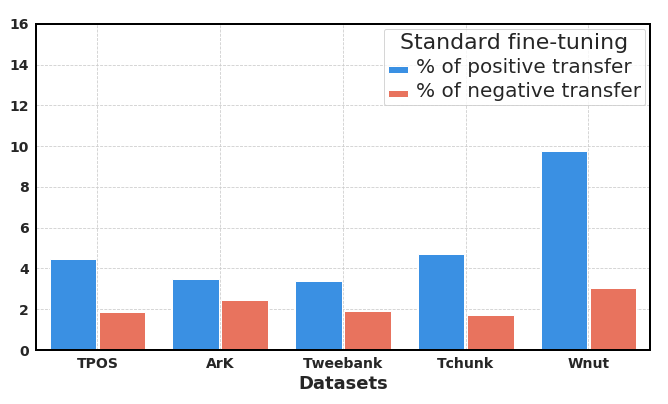
Figure 6: The percentage of negative transfer and positive transfer brought by the standard fine-tuning adaptation scheme compared to supervised training from scratch scheme.

We recall that we define positive transfer as the percentage of tokens that were wrongly predicted by random initialisation (supervised training from scratch), but the standard fine-tuning changed to the correct ones, while negative transfer represents the percentage of words that were tagged correctly by random initialisation, but using standard fine-tuning gives wrong predictions. Figure 6 shows the results on English social media datasets, first tagged with the classic supervised training scheme and then using the standard fine-tuning. Blue bars show the percentage of positive transfer and red bars give the percentage of negative transfer. We observe that even though the standard fine-tuning approach is effective since the resulting positive transfer is higher than the negative transfer in all cases, this last mitigates the final gain brought by the standard fine-tuning. For instance, for TChunk dataset, standard fine-tuning corrected $\sim$4.7% of predictions but falsified $\sim$1.7%, which reduces the final gain to $\sim$3%.

DataSet
TPoS	Award⋄	’s	its⋆	Mum	wont⋆	id⋆	Exactly
	nn	vbz	prp	nn	MD	prp	uh
	nnp	pos	prp$	uh	VBP	nn	rb
ArK	Charity⋄	I’M⋆	2pac×	2×	Titans⋆	wth×	nvr×
	noun	L	pnoun	P	Z	!	R
	pnoun	E	$	$	N	P	V
TweeBank	amazin∙	Night⋄	Angry⋄	stangs	#Trump	awsome∙	bout∙
	adj	noun	adj	propn	propn	adj	adp
	noun	propn	propn	noun	X	intj	verb
TChunk	luv×	**ROCKSTAR**THURSDAY		ONLY	Just⋄	wyd×	id⋆
	b-vp	b-np		i-np	b-advp	b-np	b-np
	i-intj	O		b-np	b-np	b-intj	i-np
Wnut	Hey⋄	Father⋄	&×	IMO×	UN	Glasgow	Supreme
	O	O	O	O	O	b-location	b-person
	b-person	b-person	i-group	b-group	b-group	b-group	b-corporation

nn=N=noun=common noun / nnp=pnoun=propn=proper noun / vbz=Verb, 3rd person singular present / pos=possessive ending / prp=personal pronoun / prp$=possessive pronoun / md=modal / VBP=Verb, non-3rd person singular present / uh=!=intj=interjection / rb=R=adverb / L=nominal + verbal or verbal + nominal / E=emoticon / $=numerical / P=pre- or postposition, or subordinating conjunction / Z=proper noun + possessive ending / V=verb / adj=adjective / adp=adposition

Table 3: Examples of falsified predictions by standard fine-tuning scheme when transferring from news domain to social media domain. Line 1: Some words from the validation-set of each data-set. Line 2: Correct labels predicted by the classic supervised setting (Random-200). Line 3: Wrong labels predicted by SFT setting. Mistake type: $\diamond$ for words with first capital letter, $\bullet$ for misspelling, $\star$ for contractions, $\times$ for abbreviations.

• ArK dataset                Tchunk dataset               Wnut dataset

Figure 7: Correlation results between $\Phi$ units’ activations before fine-tuning (columns) and after fine-tuning (rows). Brighter colours indicate higher correlation.

Qualitative Examples of Negative Transfer

We report in Table 3 concrete examples of words whose predictions were falsified when using the standard fine-tuning scheme compared to standard supervised training scheme. Among mistakes we have observed:

• Tokens with an upper-cased first letter: In news (formal English), only proper nouns start with an upper-case letter inside sentences. Consequently, when using transfer learning, the pre-trained units fail to slough this pattern which is not always respected in social media. Hence, we found that most of the tokens with an upper-cased first letter are mistakenly predicted as proper nouns (PROPN) in POS, e.g. Award, Charity, Night, etc. and as entities in NER, e.g. Father, Hey, etc., which is consistent with the findings of Seah et al. (2012): negative transfer is mainly due to conditional distribution differences between source and target domains.

• Contractions are frequently used in social media to shorten a set of words. For instance, in TPoS dataset, we found that “’s” is in most cases predicted as a “possessive ending (pos)” instead of “Verb, 3rd person singular present (vbz)”. Indeed, in formal English, “’s” is used in most cases to express the possessive form, e.g. “company’s decision”, but rarely in contractions that are frequently used in social media, e.g. “How’s it going with you?”. Similarly, “wont” is a frequent contraction for “will not”, e.g. “i wont get bday money lool”, predicted as “verb” instead of “modal (MD)” by the SFT scheme. The same for “id”, which stands for “I would”.

• Abbreviations are frequently used in social media to shorten the way a word is standardly written. We found that the standard fine-tuning scheme stumbles on abbreviations predictions, e.g. 2pac (Tupac), 2 (to), ur (your), wth (what the hell) and nvr (never) in ArK dataset; and luv (love) and wyd (what you doing?) in TChunk dataset.

• Misspellings: Likewise, we found that the standard fine-tuning scheme often gives wrong predictions for misspelt words, e.g. awsome, bout, amazin.

7.1.2 Quantifying the change of individual pretrained neurons

To visualise the bias phenomenon occurring when using the standard fine-tuning scheme, we quantify the charge of individual neurons. Precisely, we plot the asymmetric correlation matrix $\mathbf{C}$ (The method described in section 4.2.1) between the $\Phi$ layer’s units before and after fine-tuning for each social media dataset (ArK for POS, TChunk for CK and WNUT-17 for NER). From the resulting correlation matrices illustrated in Figure 7, we can observe the diagonal representing the charge of each unit, with most of the units having a high charge (light colour), alluding the fact that every unit after fine-tuning is highly correlated with itself before fine-tuning. Hypothesising that high correlation in the diagonal entails high bias, the results of this experiment confirm our initial motivation that pre-trained units are highly biased to what they have learnt in the source-dataset, making them limited to learn some patterns that are specific to the target-dataset. Our remarks were confirmed recently in the recent work of Merchant et al. (2020) who also found that fine-tuning is a “conservative process”.

7.1.3 Visualising the Evolution of Pretrained Neurons Stimulus during Fine-tuning

Here, we give concrete visualisations of the evolution of pretrained neurons stimulus during fine-tuning when transferring from the news domain to the social media domain. Following the method described in section 4.2.2, we plot the matrices of top-10 words activating each neuron $j$, positively ($\mathbf{A}^{(j)}_{best+}$) or negatively ($\mathbf{A}^{(j)}_{best-}$). The results are plotted in Figure 8 for ArK (POS) dataset and Figure 9 for TweeBank dataset (POS). Rows represent the top-10 words from the target dataset activating each unit, and columns represent fine-tuning epochs; before fine-tuning in column 0 (at this stage the model is only trained on the source-dataset), and during fine-tuning (columns 5 to 20). Additionally, to get an idea about each unit’s stimulus on source dataset, we also show, in the first column (Final-WSJ), top-10 words from the source dataset activating the same unit before fine-tuning. In the following, we describe the information encoded by each provided neuron.

• Ark - POS: (Figure 8)

  • Unit-196 is sensitive to contractions containing an apostrophe regardless of the contraction’s class. However, unlike news, in social media and particularly ArK dataset, apostrophes are used in different cases. For instance i’m, i’ll and it’s belong to the class “L” that stands for “nominal + verbal or verbal + nominal”, while the contractions can’t and don’t belong to the class “Verb”.

  • Unit-64 is sensitive to plural proper nouns on news-domain before fine-tuning, e.g. Koreans and Europeans, and also on ArK during fine-tuning, e.g. Titans and Patriots. However, in ArK dataset, “Z” is a special class for “proper noun + possessive ending”, e.g. Jay’s mum, and in some cases the apostrophe is omitted, e.g. Fergusons house for Ferguson’s house, which thus may bring ambiguity with plural proper nouns in formal English. Consequently, unit-64, initially sensitive to plural proper nouns, is also firing on words from the class “Z”, e.g. Timbers (Timber’s).

  • Unit-196: ArK dataset

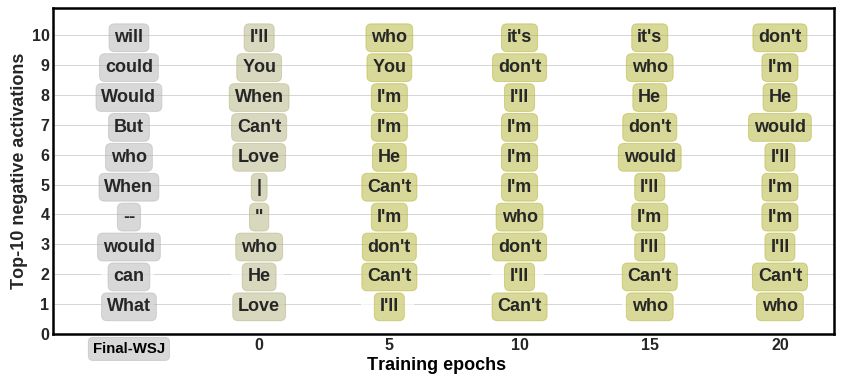
  • Unit-64: ArK dataset

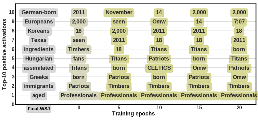
  Figure 8: Individual units activations before and during fine-tuning from ArK POS dataset. For each unit we show Top-10 words activating the said unit. The first column: top-10 words from the source validation-set (WSJ) before fine-tuning, Column 0: top-10 words from the target validation-set (ArK) before fine-tuning. Columns 5 to 20: top-10 words from the target validation-set during fine-tuning epochs.

• Tweebank - POS: (Figure 9)

  • Unit-37 is sensitive before and during fine-tuning on plural nouns, such as gazers and feminists. However, it is also firing on the word slangs because of the s ending, which is in fact a proper noun. This might explain the wrong prediction for the word slangs (noun instead of proper noun) given by the standard fine-tuning scheme (Table 3).

  • Unit-169 is highly sensitive to proper nouns (e.g. George and Washington) before fine-tuning, and to words with capitalised first-letter whether the word is a proper noun or not (e.g. Man and Father) during fine-tuning on the TweeBank dataset. Which may explain the frequent wrong predictions of tokens with upper-cased first letter as proper nouns by the standard fine-tuning scheme.

  • Unit-37: Tweebank dataset

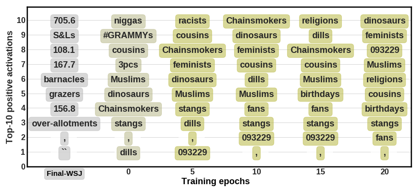
  • Unit-169: Tweebank dataset

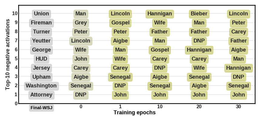
  Figure 9: Individual units activations before and during fine-tuning on Tweebank POS dataset. For each unit we show Top-10 words activating the said unit. The first column: top-10 words from the source validation-set (WSJ) before fine-tuning, Column 0: top-10 words from the target validation-set (Tweebank) before fine-tuning. Columns 5 to 20: top-10 words from the target validation-set during fine-tuning epochs.

7.2 PretRand’s Results

In this section, we present PretRand’s performance on POS, CK, NER and MST tasks on social media datasets:

1. We compare PretRand’s to baseline methods, in the scenario in which contextual representations (ELMo) are not used (section 7.2.1).

2. We measure the importance of each component of PretRand on the overall performance (section 7.2.2).

3. We investigate the impact of incorporating contextual representations, on baselines vs PretRand (section 7.2.3).

4. We compare PretRand to best state-of-the-art approaches (section 7.2.4).

5. We investigate in which scenarios PretRand is most advantageous (section 7.2.5).

6. We assess the impact of PretRand on the hidden negative transfer compared to the standard fine-tuning (section 7.2.6)

7.2.1 Comparison with Baseline Methods

In this section we assess the performance of PretRand through a comparison to six baseline-methods, illustrated in Figure 10. First, since PretRand is an amelioration of the standard fine-tuning (SFT) adaptation scheme, we mainly compare it to the SFT baseline. Besides, we assess whether the gain brought by PretRand is due to the increase in the number of parameters; thus we also compare with the standard supervised training scheme with a wider model. Finally, the final predictions of PretRand are the combination of the predictions of the two branches, randomly initialised and pretrained, which can make one think about ensemble methods (Dietterich, 2000). Thus we also compare with ensemble methods. The following items describe the different baseline-methods used for comparison:

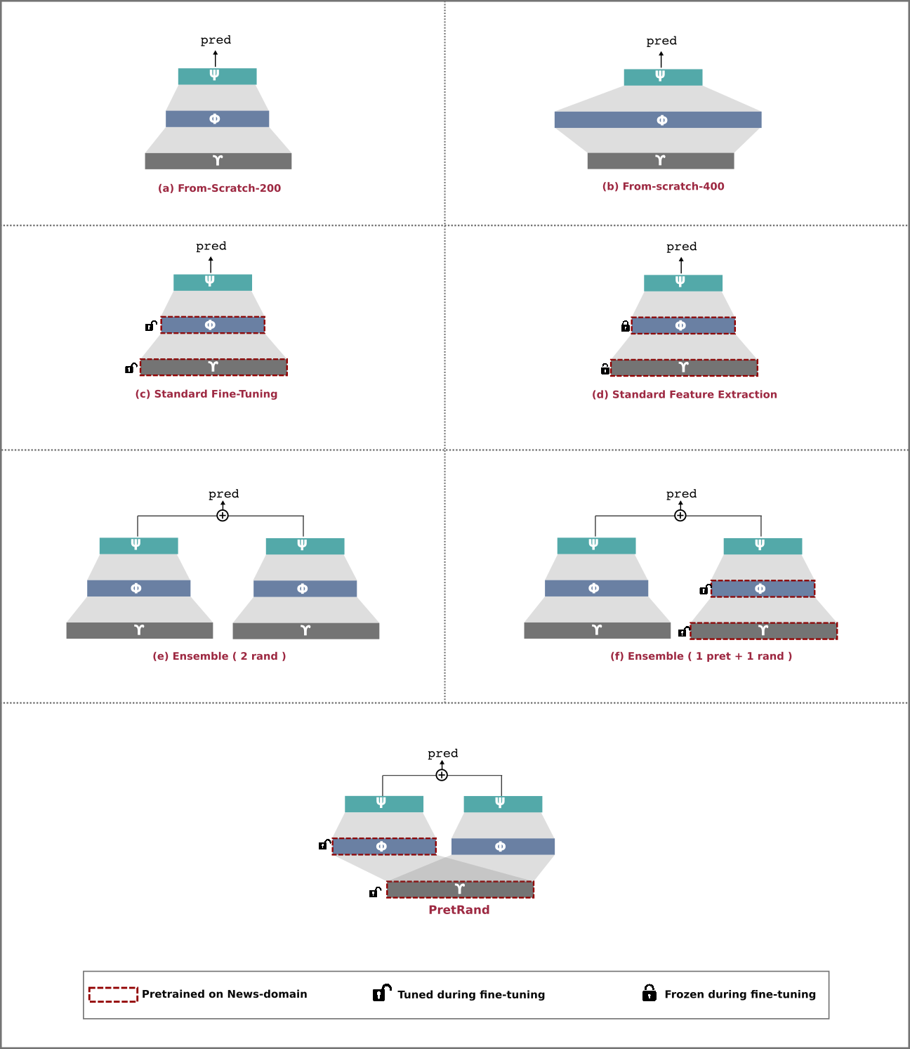
Figure 10: Illustrative schemes of baseline-methods and PretRand.

• (a) From-scratch₂₀₀: The base model described in section 1, trained from scratch using the standard supervised training scheme on social media dataset (without transfer learning). Here the number 200 refers to the dimensionality of the biLSTM network in the $\mathbf{FE}$ ($\Phi$).

• (b) From-scratch₄₀₀: The same as “From-scratch₂₀₀” baseline but with 400 instead of 200 biLSTM units in the $\mathbf{FE}$. Indeed, by experimenting with this baseline, we aim to highlight that the impact of PretRand is not due to the increase in the number of parameters.

• (c) Standard Fine-tuning (SFT): Pre-training the base model on the source-dataset, followed by an adaptation on the target-dataset with the standard fine-tuning scheme (section 4).

• (d) Standard Feature Extraction (SFE): The same as SFT, but the pretrained parameters are frozen during fine-tuning on the social media datasets.

• (e) Ensemble (2 rand): Averaging the predictions of two base models that are randomly initialised and learnt independently on the same target dataset, but with a different random initialisation.

• (f) Ensemble (1 pret + 1 rand): same as the previous but with one pre-trained on the source-domain (SFT baseline) and the other randomly initialised (From-scratch₂₀₀ baseline).

Method	#params	POS (acc.)			CK (acc.)	NER (F1)		aNRG
		TPoS	ArK	TweeBank	TChunk	WNUT
From-scratch200	$1\times$	86.82	91.10	91.66	85.96	36.75		0
From-scratch400	$1.03\times$	86.61	91.31	91.81	87.11	38.64		+2.7
1-11 Feature Extraction	$1\times$	86.08	85.25	87.93	81.49	27.83		-32.4
Fine-Tuning	$1\times$	89.57	92.09	93.23	88.86	41.25		+15.7
1-11 Ensemble (2 rand)	$2\times$	88.98	91.45	92.26	86.72	39.54		+7.5
Ensemble (1p+1r)	$2\times$	88.74	91.67	93.06	88.78	42.66		+13.4
1-11 PretRand	$1.02\times$	91.27	93.81	95.11	89.95	43.12		+28.8

Method	#params		MST (acc.)			aNRG
			Serbian	Slovene	Croatian
From-scratch200	$1\times$		86.18	84.42	85.67	0
From-scratch400	$1.03\times$		86.05	84.37	85.77	-0.2
1-11 Feature Extraction	$1\times$		73.56	70.22	79.11	-76.1
Fine-Tuning	$1\times$		87.59	88.76	88.79	+19.9
1-11 Ensemble (2 rand)	$2\times$		87.01	84.67	86.05	+3.4
Ensemble (1p+1r)	$2\times$		87.96	88.54	88.87	+20.6
1-11 PretRand	$1.02\times$		88.21	90.01	90.23	+27.5

Table 4: Comparison of PretRand to baselines methods. Comparison of our method to baselines in terms of token-level accuracy for POS, CK and MST and entity-level F1 for NER (in %) on social media test-sets. In the second column (#params), we highlight the number of parameters of each method compared to the reference From-scratch₂₀₀ baseline. In the last column, we report the aNRG score of each method compared to the reference From-scratch₂₀₀. Best score per dataset is in bold, and the second best score is underlined.

Method	POS			CK	NER	MST
	TPoS	ArK	TweeBank	TChnuk	WNUT	Serbian	Slovene	Croatian
PretRand	91.27	93.81	95.11	89.95	43.12	88.21	90.01	90.23
-learnVect	91.11	93.41	94.71	89.64	42.76	88.01	89.83	90.12
-learnVect -random++	90.84	93.56	94.26	89.05	42.70	87.85	89.39	89.51
-learnVect -random++ -l2 norm	90.54	92.19	93.28	88.66	41.84	87.66	88.64	88.49

Table 5: Diagnostic analysis of the importance of each component in PretRand. Accuracy for POS, CK and MST and F1 for NER (in %) when progressively ablating PretRand components.

We summarise the comparison of PretRand to the above baselines in Tables 4. In the first table, we report the results of POS, CK and NER English social media datasets. In the second table, we report the results of MST on Serbian, Slovene and Croatian social media datasets. We compare the different approaches using the aNRG metric (see equation 12) compared to the reference From-scratch₂₀₀. First, we observe that PretRand outperforms the popular standard fine-tuning baseline significantly by +13.1 aNRG (28.8-15.7). More importantly, PretRand outperforms the challenging Ensemble method across all tasks and datasets and by +15.4 (28.8-13.4) on aNRG, while using much fewer parameters. This highlights the difference between our method and the ensemble methods. Indeed, in addition to normalisation and weighting vectors, PretRand is conceptually different since the random and pretrained branches share the WRE component. Also, the results of From-scratch₄₀₀ compared to From-scratch₂₀₀ baseline confirm that the gain brought by PretRand is not due to the supplement parameters. In the following (section 7.2.2), we show that the gain brought by PretRand is mainly due to the shared word representation in combination with the normalisation and the learnable weighting vectors during training. Moreover, a key asset of PretRand is that it uses only 0.02% more parameters compared to the fine-tuning baseline.

7.2.2 Diagnostic Analysis of the Importance of PretRand’s Components

While in the precedent experiment we reported the best performance of PretRand, here we carry out an ablation study to diagnose the importance of each component in our proposed approach. Specifically, we successively ablate the main components of PretRand, namely, the learnable weighting vectors (learnVect), the longer training of the random branch (random++) and the normalisation ($\ell_{2}$-norm). From the results in Table 5, we can first observe that ablating each of them successively degrades the results across all datasets, which highlights the importance of each component. Second, the results are only marginally better than the SFT when ablating the three components from PretRand (the last line in Table 5). Third, ablating the normalisation layer significantly hurts the performance across all data-sets, confirming the importance of this step of making the two branches more competitive.

Method	#	Char⋄⋆	Word∙⋆	ELMo∙×	POS (acc.)			CK (acc.)	NER (F1.)	MST (acc.)
					TPoS	ArK	TweeB	TChunk	WNUT	Croatian
From-scratch	A				82.16	87.66	88.30	84.56	17.99	83.26
2-11	B				85.21	88.34	90.63	84.17	36.58	80.03
2-11	C				86.82	91.10	91.66	85.96	36.75	85.67
2-11	D				88.35	90.62	92.51	89.61	34.35	86.34
2-11	E				89.01	91.48	93.21	88.48	33.99	86.94
2-11	F				89.31	91.57	93.60	89.39	40.16	85.97
2-11	G				90.01	92.09	93.73	88.99	41.57	86.79
SFT	A				86.87	88.30	89.26	87.28	21.88	86.19
2-11	B				87.61	89.63	92.31	87.19	41.50	83.07
2-11	C				89.57	92.09	93.23	88.86	41.25	88.79
2-11	D				88.02	90.32	93.04	89.69	44.21	88.25
2-11	E				90.18	91.81	93.53	90.55	43.98	88.76
2-11	F				88.87	91.83	93.71	88.82	45.73	89.28
2-11	G				90.27	92.73	94.19	90.75	46.59	89.00
PretRand	A				88.01	90.11	91.16	88.49	22.12	87.63
2-11	B				88.56	90.56	93.99	88.55	42.87	93.67
2-11	C				91.27	93.81	95.11	89.95	43.12	90.23
2-11	D				88.15	90.26	93.41	89.84	45.54	88.94
2-11	E				91.12	92.94	94.89	91.36	45.13	89.93
2-11	F				89.54	93.16	94.15	89.37	46.62	90.16
2-11	G				91.45	94.18	95.22	91.49	47.33	90.33

Table 6: Diagnosis analysis of the impact of ELMo contextual representations.. From-scratch, SFT and PretRand results, on social media test-sets, when ablating one or more type of representations. $\diamond$: from scratch, $\bullet$: pre-loaded, $\star$: trained, $\times$: frozen.

7.2.3 Incorporating Contextualised Word Representations

So far in our experiments, we have used only the standard pre-loaded words embeddings and character-level embeddings in the $\mathbf{WRE}$ component. Here, we perform a further experiment that examines the effect of incorporating the ELMo contextualised word representations (Peters et al., 2018) in different tasks and training schemes (From-scratch, SFT and PretRand). Specifically, we carry out an ablation study of $\mathbf{WRE}$’s representations, namely, the standard pre-loaded words embeddings (word), character-level embeddings (char) and ELMo contextualised embeddings (ELMo). The ablation leads to 7 settings; in each, one or more representations are ablated. Results are provided in Table 6, “” means that the corresponding representation is used and “” means that it is ablated. For instance, in setting A only character-level representation is used.

Three important observations can be highlighted. First, in training from scratch scheme, as expected, contextualised ELMo embeddings have a considerable effect on all datasets and tasks. For instance, setting D (using ELMo solely) outperforms setting C (standard concatenation between character-level and word-level embeddings), considerably on Chunking and NER and slightly on POS tagging (except ArK). Furthermore, combining ELMo embeddings to the standard concatenation between character-level and word-level embeddings (setting G) gives the best results across all tasks and social media datasets. Second, when applying our transfer learning approaches, whether SFT or PretRand, the gain brought by ELMo embeddings (setting G) compared to standard concatenation between character-level and word-level embeddings (setting C) is slight on POS tagging (in average, SFT: +0.76% , PretRand: +0.22%) and Croatian MS tagging (SFT: +0.21% , PretRand: +0.10%), whilst is considerable on CK (SFT: +1.89% , PretRand: +1.54%) and major on NER (SFT: +5.3% , PretRand: +4.2%). Finally, it should be pointed out that using ELMo slows down the training and inferences processes; it becomes 10 times slower.

Method	POS (acc.)			CK (acc.)	NER (F1.)	MST (acc.)
	TPoS	ArK	TweeBank	TChunk	WNUT	Sr	Sl	Hr
CRF (Ritter et al., 2011)⋆	88.3	n/a	n/a	87.5	n/a	n/a	n/a	n/a
1-9 GATE (Derczynski et al., 2013)⋆	88.69	n/a	n/a	n/a	n/a	n/a	n/a	n/a
1-9 GATE-bootstrap⋆	90.54	n/a	n/a	n/a	n/a	n/a	n/a	n/a
1-9 ARK tagger (Owoputi et al., 2013)⋆	90.40	93.2	94.6	n/a	n/a	n/a	n/a	n/a
1-9 TPANN (Gui et al., 2017)${}^{\star~{}\times}$	90.92	92.8	n/a	n/a	n/a	n/a	n/a	n/a
1-9 Flairs (Akbik et al., 2019)⋄	n/a	n/a	n/a	n/a	49.59	n/a	n/a	n/a
1-9 MDMT (Mishra, 2019)${}^{\diamond~{}\times}$	91.70	91.61	92.44	n/a	49.86	n/a	n/a	n/a
1-9 DA-LSTM (Gu and Yu, 2020)×	89.16	n/a	n/a	n/a	n/a	n/a	n/a	n/a
1-9 DA-BERT (Gu and Yu, 2020)${}^{\bullet~{}\times}$	91.55	n/a	n/a	n/a	n/a	n/a	n/a	n/a
1-9 1-9 BertTweet (Nguyen et al., 2020)${}^{\bullet~{}\star}$	90.1	94.1	95.2	n/a	54.1	n/a	n/a	n/a
1-9 UH&UC	n/a	n/a	n/a	n/a	n/a	90.00	88.4	88.7
PretRand (our best)⋄	91.45	94.18	95.22	91.49	47.33	88.21	90.01	90.33

Table 7: Comparison of PretRand to the best published state-of-the-art methods in terms of token-level accuracy for POS, CK and MST and F1 for NER (in %) on social media datasets. $\diamond$: use of contextualised representations. $\bullet$: use of BERT pretrained model. $\star$: use of normalisation dictionaries, regular expressions or external knowledge. $\times$: use of a CRF classifier on top of the neural model.

7.2.4 Comparison to state-of-the-art

We compare our results to the following state-of-the-art methods:

• CRF (Ritter et al., 2011) is a Conditional Random Fields (CRF) (Lafferty et al., 2001) based model with Brown clusters. It was jointly trained on a mixture of hand-annotated social-media texts and labelled data from the news domain, in addition to annotated IRC chat data (Forsythand and Martell, 2007).

• GATE (Derczynski et al., 2013) is a model based on Hidden Markov Models with a set of normalisation rules, external dictionaries, lexical features and out-of-domain annotated data. The authors experimented it on TPoS, with WSJ and 32K tokens from the NPS IRC corpus. They also proposed a second variety (GATE-bootstrap) using 1.5M additional training tokens annotated by vote-constrained bootstrapping.

• ARK tagger (Owoputi et al., 2013) is a model based on first-order Maximum Entropy Markov Model with greedy decoding. Brown Clusters, regular expressions and careful hand-engineered lexical features were also used.

• TPANN (Gui et al., 2017) is a biLSTM-CRF model that uses adversarial pre-training (Ganin et al., 2016) to leverage huge amounts of unlabelled social media texts, in addition to labelled datasets from the news domain. Next, the pretrained model is further fine-tuned on social media annotated examples. Also, regular expressions were used to tag Twitter-specific classes (hashtags, usernames, urls and @-mentions).

• Flairs (Akbik et al., 2019) is a biLSTM-CRF sequence labelling architecture fed with the Pooled Contextual Embeddings (Akbik et al., 2018) (pre-trained on character-level language models).

• UH&CU (Silfverberg and Drobac, 2018) is a biLSTM-based sequence labelling model for MST, jointly trained on formal and informal texts. It is similar to our base model, but used 2-stacked biLSTM layers. In addition, the particularity of UH&CU is that the final predictions are generated as character sequences using an LSTM decoder, i.e. a character for each morpho-syntactic feature instead of an atomic label.

• Multi-dataset-multi-task (MDMT) (Mishra, 2019) consists in a multi-task training of 4 NLP tasks: POS, CK, super sense tagging and NER, on 20 Tweets datasets 7 POS, 10 NER, 1 CK, and 2 super sense–tagged datasets. The model is based on a biLSTM-CRF architecture and words representations are based on the pre-trained ELMo embeddings.

• Data Annealing (DA) (Gu and Yu, 2020) is a fine-tuning approach similar to our SFT baseline, but the passage from pretraining to fine-tuning is performed gradually, i.e. the training starts with only formal text data (news) at first; then, the proportion of the informal text data (social media) is gradually increased during the training process. They experiment with two architectural varieties, a biLSTM-based architecture (DA-LSTM) and a Transformer-based architecture (DA-BERT). In the last variety, the model is initialised with BERT_base pretrained model (110 million parameters). A CRF classifier is used as a classifier on the top of both varieties, biLSTM and BERT.

• BertTweet (Nguyen et al., 2020) is a large-scale model pretrained on an 80GB corpus of 850M English Tweets. The model is trained using BERT_base (Devlin et al., 2019) architecture and following the pretraining procedure of RoBERTa (Liu et al., 2019b). In order to perform POS tagging and NER, a randomly initialised linear prediction layer is appended on top of the last Transformer layer of BERTweet, and then the model is fine-tuned on target tasks examples. In addition, lexical dictionaries were used to normalise social media texts.

From Table 7, we observe that PretRand outperforms best state-of-the-art results on POS tagging datasets (except TPoS), Chunking (+4%), Slovene (+1.5%) and Croatian (1.6%) MS tagging. However, it performs worse than UH&UC for Serbian MS tagging. This could be explained by the fact that the Serbian source dataset (news) is small compared to Slovene and Croatian, reducing the gain brought by pretraining and thus that brought by PretRand. Likewise, Akbik et al. (2019) outperforms our approach on NER task, in addition to using a CRF on top of the biLSTM layer, they used Contextual string embeddings that have been shown to perform better on NER than ELMo (Akbik et al., 2019). Also, MDMT outperforms PretRand slightly on TPoS dataset. We can observe that BERT-based approaches (DA-BERT and BertTweet) achieve strong results, especially on NER, where BertTweet begets the best state-of-the-art score. Finally, we believe that adding a CRF classification layer on top of our models will boost our results (like TPANN, MDMT, DA-LSTM and DA-BERT), as it is able to model strong dependencies between adjacent words.

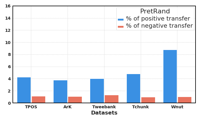
Figure 11: Positive and negative transfers brought by SFT (left) and PretRand (Right) compared to the standard supervised training scheme (From-scratch).

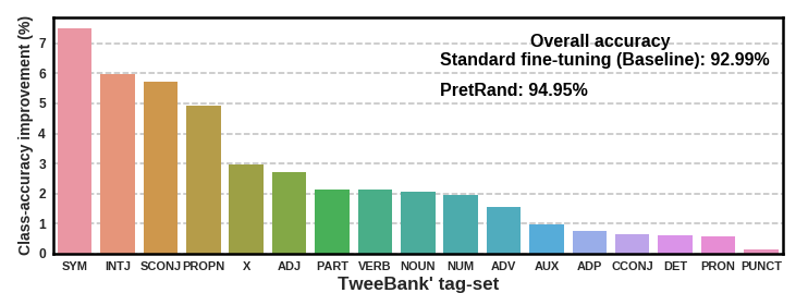
Figure 12: Sorted class-accuracy improvement (%) on TweeBank of PretRand compared to fine-tuning.

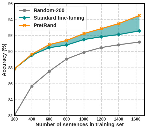
Figure 13: Performances (on dev-set of TweeBank) according different training-set sizes for the target-dataset. Transparent green highlights the difference between our PretRand and standard fine-tuning.

7.2.5 When and where PretRand is most Beneficial?

Here, we attempt to examine in which scenarios PretRand is most beneficial. We firstly explore in Figure 12, which class from TweeBank dataset benefits more from PretRand compared to SFT. After that, we evaluate in Figure 13 the gain on accuracy brought by PretRand compared to SFT, according to different target-datasets’ sizes. We observe that PretRand has desirably a bigger gain with bigger target-task datasets, which clearly means that the more target training-data, the more interesting our method will be. This observation may be because the random branch needs sufficient amounts of target training samples to become more competitive with the pretrained one.

7.2.6 Negative Transfer: PretRand vs SFT

Here, we resume the negative transfer experiment performed in section 7.1.1 . Precisely, we compare the results of PretRand to those of SFT. We show in Figure 11 the results on English social media datasets, first tagged with the classic training scheme (From-scratch₂₀₀) and then using SFT in the left plot (or using PretRand in the right plot). Blue bars show the percentage of positive transfer, i.e. predictions that were wrong, but the SFT (or PretRand) changed to the correct ones, and red bars give the percentage of negative transfer, i.e. predictions that were tagged correctly by From-scratch₂₀₀, but using SFT (or PretRand) gives the wrong predictions. We observe the high impact of PretRand on diminishing negative transfer vis-a-vis to SFT. Precisely, PretRand increases positive transfer by $\sim$0.45% and decreases the negative transfer by $\sim$0.94% on average.

8 Conclusion and Perspectives

We have started by analysing the results of the standard fine-tuning adaptation scheme of transfer learning. First, we were interested in the hidden negative transfer that arises when transferring from the news domain to the social media domain. Indeed, negative transfer has only seldom been tackled in sequential transfer learning works in NLP. In addition, earlier research papers evoke negative transfer only when the source domain has a negative impact on the target model. We found that despite the positive gain brought by transfer learning from the high-resource news domain to the low-resource social media domain, the hidden negative transfer mitigates the final gain brought by transfer learning. Second, we carried out an interpretive analysis of the evolution, during fine-tuning, of pretrained representations. We found that while fine-tuning necessarily makes some changes during fine-tuning on social media datasets, pretrained neurons still biased by what they have learnt in the source domain. In simple words, pretrained neurons tend to conserve much information from the source domain. Some of this information is undoubtedly beneficial for the social media domain (positive transfer), but some of it is indeed harmful (negative transfer). We hypothesise that this phenomenon of biased neurons restrains the pretrained model from learning some new features specific to the target domain (social media).

Stemming from our analysis, we have introduced a novel approach,PretRand, to overcome this problem using three main ideas: adding random units and jointly learn them with pre-trained ones; normalising the activations of both to balance their different behaviours; applying learnable weights on both predictors to let the network learn which of random or pre-trained one is better for every class. The underlying idea is to take advantage of both, target-specific features from the former and general knowledge from the latter. We carried out experiments on domain adaptation for 4 tasks: part-of-speech tagging, morpho-syntactic tagging, chunking and named entity recognition. Our approach exhibits performances significantly above standard fine-tuning scheme and is highly competitive when compared to the state-of-the-art.

Perspectives

We believe that many prosperous directions should be addressed in future research. More extensive experiments would be interesting to better understand the phenomenon of the hidden negative transfer and to confirm our observations. First, one can investigate the impact of the model’s hyper-parameters (size, activation functions, learning rate, etc.) as well as regulation methods (dropout, batch normalisation, weights decay, etc.). Second, we suppose that the hidden negative transfer would be more prominent when the target dataset is too small since the pre-learned source knowledge will be more preserved. Hence, it would be interesting to assess the impact of target-training size. Third, a promising experiment would be to study the impact of the similarity between the source and the target distributions. Fourth, a fruitful direction would be to explain this hidden negative transfer using explainability methods. Notably, one can use influence functions (Han et al., 2020) to identify source training examples that are responsible for the negative transfer. Further, to identify text pieces of the evaluated sentence that justify a prediction with a negative transfer, one can use for instance gradients based methods (Shrikumar et al., 2017).

Concerning the quantification of the change of pretrained individual neurons, it would also be interesting to perform a representation-level similarity analysis to gain more insights, as it has been shown by Wu et al. (2020) that representation-level similarity measures the distributional similarity while individual-level measures local similarity.

PretRand’s good results on sequence labelling tasks suggest to consider other kinds of NLP tasks, e.g. sequence-to-sequence and text classification tasks. Further, as negative transfer, and thus bias, is highly arising when transferring between less-related source-target domains (Wang et al., 2019), PretRand’s impact would be more interesting for cross-lingual transfer. Also, in this work, we experimented PretRand adaptation scheme on models pre-trained in a supervised manner, an important step forward is to examine its scalability with other pretraining methods, e.g. adversarial or unsupervised pretraining. In addition, the increasing omnipresence of Transformers architectures in a wide range of NLP tasks, due to their improved performances, motivates us to experiment with Transformer-based architecture instead of LSTM-based one. Last, a propitious continuity of our work to tackle the bias problem, would be to identify automatically biased neurons in the pre-trained model and proceed to a pruning of the most biased ones before fine-tuning.

References

- Adi et al. (2016) Yossi Adi, Einat Kermany, Yonatan Belinkov, Ofer Lavi, and Yoav Goldberg. 2016. Fine-grained analysis of sentence embeddings using auxiliary prediction tasks. Proceedings of ICLR Conference Track.
- Akbik et al. (2019) Alan Akbik, Tanja Bergmann, and Roland Vollgraf. 2019. Pooled contextualized embeddings for named entity recognition. In Proceedings of the 2019 Conference of the North American Chapter of the Association for Computational Linguistics: Human Language Technologies, Volume 1 (Long and Short Papers), pages 724–728.
- Akbik et al. (2018) Alan Akbik, Duncan Blythe, and Roland Vollgraf. 2018. Contextual string embeddings for sequence labeling. In Proceedings of the 27th International Conference on Computational Linguistics, pages 1638–1649.
- Bau et al. (2019) Anthony Bau, Yonatan Belinkov, Hassan Sajjad, Nadir Durrani, Fahim Dalvi, and James Glass. 2019. Identifying and controlling important neurons in neural machine translation. ICLR.
- Baumann and Pierrehumbert (2014) Peter Baumann and Janet B Pierrehumbert. 2014. Using resource-rich languages to improve morphological analysis of under-resourced languages. In LREC, pages 3355–3359.
- Belinkov and Glass (2019) Yonatan Belinkov and James Glass. 2019. Analysis methods in neural language processing: A survey. Transactions of the Association for Computational Linguistics, 7:49–72.
- Bengio et al. (2003) Yoshua Bengio, Réjean Ducharme, Pascal Vincent, and Christian Jauvin. 2003. A neural probabilistic language model. Journal of machine learning research, 3(Feb):1137–1155.
- Bojanowski et al. (2017) Piotr Bojanowski, Edouard Grave, Armand Joulin, and Tomas Mikolov. 2017. Enriching word vectors with subword information. Transactions of the Association for Computational Linguistics, 5:135–146.
- Cao et al. (2018) Zhangjie Cao, Mingsheng Long, Jianmin Wang, and Michael I Jordan. 2018. Partial transfer learning with selective adversarial networks. In Proceedings of the IEEE Conference on Computer Vision and Pattern Recognition, pages 2724–2732.
- Cer et al. (2018) Daniel Cer, Yinfei Yang, Sheng-yi Kong, Nan Hua, Nicole Limtiaco, Rhomni St John, Noah Constant, Mario Guajardo-Cespedes, Steve Yuan, Chris Tar, et al. 2018. Universal sentence encoder for english. In Proceedings of the 2018 Conference on Empirical Methods in Natural Language Processing: System Demonstrations, pages 169–174.
- Che et al. (2018) Wanxiang Che, Yijia Liu, Yuxuan Wang, Bo Zheng, and Ting Liu. 2018. Towards better ud parsing: Deep contextualized word embeddings, ensemble, and treebank concatenation. In Proceedings of the CoNLL 2018 Shared Task: Multilingual Parsing from Raw Text to Universal Dependencies, pages 55–64.
- Chen et al. (2018) Xilun Chen, Yu Sun, Ben Athiwaratkun, Claire Cardie, and Kilian Weinberger. 2018. Adversarial deep averaging networks for cross-lingual sentiment classification. Transactions of the Association for Computational Linguistics, 6:557–570.
- Chen et al. (2019) Xinyang Chen, Sinan Wang, Bo Fu, Mingsheng Long, and Jianmin Wang. 2019. Catastrophic forgetting meets negative transfer: Batch spectral shrinkage for safe transfer learning. In Advances in Neural Information Processing Systems, pages 1908–1918.
- Clark et al. (2019) Kevin Clark, Urvashi Khandelwal, Omer Levy, and Christopher D Manning. 2019. What does bert look at? an analysis of bert’s attention. arXiv preprint arXiv:1906.04341.
- Coates and Ng (2011) Adam Coates and Andrew Y Ng. 2011. Selecting receptive fields in deep networks. In Advances in neural information processing systems, pages 2528–2536.
- Conneau et al. (2017) Alexis Conneau, Douwe Kiela, Holger Schwenk, Loïc Barrault, and Antoine Bordes. 2017. Supervised learning of universal sentence representations from natural language inference data. In Proceedings of the 2017 Conference on Empirical Methods in Natural Language Processing, pages 670–680.
- Conneau et al. (2018) Alexis Conneau, Germán Kruszewski, Guillaume Lample, Loïc Barrault, and Marco Baroni. 2018. What you can cram into a single $ &!#* vector: Probing sentence embeddings for linguistic properties. In Proceedings of the 56th Annual Meeting of the Association for Computational Linguistics (Volume 1: Long Papers), pages 2126–2136.
- Derczynski et al. (2017) Leon Derczynski, Eric Nichols, Marieke van Erp, and Nut Limsopatham. 2017. Results of the wnut2017 shared task on novel and emerging entity recognition. In Proceedings of the 3rd Workshop on Noisy User-generated Text, pages 140–147.
- Derczynski et al. (2013) Leon Derczynski, Alan Ritter, Sam Clark, and Kalina Bontcheva. 2013. Twitter part-of-speech tagging for all: Overcoming sparse and noisy data. In Proceedings of the International Conference Recent Advances in Natural Language Processing RANLP 2013, pages 198–206.
- Devlin et al. (2019) Jacob Devlin, Ming-Wei Chang, Kenton Lee, and Kristina Toutanova. 2019. Bert: Pre-training of deep bidirectional transformers for language understanding. In Proceedings of the 2019 Conference of the North American Chapter of the Association for Computational Linguistics: Human Language Technologies, Volume 1 (Long and Short Papers), pages 4171–4186.
- Dhingra et al. (2017) Bhuwan Dhingra, Hanxiao Liu, Ruslan Salakhutdinov, and William W Cohen. 2017. A comparative study of word embeddings for reading comprehension. arXiv preprint arXiv:1703.00993.
- Dietterich (2000) Thomas G Dietterich. 2000. Ensemble methods in machine learning. In International workshop on multiple classifier systems, pages 1–15. Springer.
- Duong (2017) Long Duong. 2017. Natural language processing for resource-poor languages. Ph.D. thesis, University of Melbourne.
- Eisenstein (2019) Jacob Eisenstein. 2019. Measuring and modeling language change. In Proceedings of the 2019 Conference of the North American Chapter of the Association for Computational Linguistics: Tutorials, pages 9–14.
- Fecht et al. (2019) Pascal Fecht, Sebastian Blank, and Hans-Peter Zorn. 2019. Sequential transfer learning in nlp for german text summarization.
- Forsythand and Martell (2007) Eric N Forsythand and Craig H Martell. 2007. Lexical and discourse analysis of online chat dialog. In Semantic Computing, 2007. ICSC 2007. International Conference on, pages 19–26. IEEE.
- Ganin et al. (2016) Yaroslav Ganin, Evgeniya Ustinova, Hana Ajakan, Pascal Germain, Hugo Larochelle, François Laviolette, Mario Marchand, and Victor Lempitsky. 2016. Domain-adversarial training of neural networks. The Journal of Machine Learning Research, 17(1):2096–2030.
- Ge et al. (2014) Liang Ge, Jing Gao, Hung Ngo, Kang Li, and Aidong Zhang. 2014. On handling negative transfer and imbalanced distributions in multiple source transfer learning. Statistical Analysis and Data Mining: The ASA Data Science Journal, 7(4):254–271.
- Giorgi and Bader (2018) John M Giorgi and Gary D Bader. 2018. Transfer learning for biomedical named entity recognition with neural networks. Bioinformatics, 34(23):4087–4094.
- Girshick et al. (2014) Ross Girshick, Jeff Donahue, Trevor Darrell, and Jitendra Malik. 2014. Rich feature hierarchies for accurate object detection and semantic segmentation. In Proceedings of the IEEE conference on computer vision and pattern recognition, pages 580–587.
- Graves et al. (2013) Alex Graves, Navdeep Jaitly, and Abdel-rahman Mohamed. 2013. Hybrid speech recognition with deep bidirectional lstm. In 2013 IEEE workshop on automatic speech recognition and understanding, pages 273–278. IEEE.
- Gu and Yu (2020) Jing Gu and Zhou Yu. 2020. Data annealing for informal language understanding tasks. EMNLP2020 Findings.
- Gui et al. (2018) Lin Gui, Ruifeng Xu, Qin Lu, Jiachen Du, and Yu Zhou. 2018. Negative transfer detection in transductive transfer learning. International Journal of Machine Learning and Cybernetics, 9(2):185–197.
- Gui et al. (2017) Tao Gui, Qi Zhang, Haoran Huang, Minlong Peng, and Xuan-Jing Huang. 2017. Part-of-speech tagging for twitter with adversarial neural networks. In Proceedings of the 2017 Conference on Empirical Methods in Natural Language Processing, pages 2411–2420.
- Han et al. (2020) Xiaochuang Han, Byron C Wallace, and Yulia Tsvetkov. 2020. Explaining black box predictions and unveiling data artifacts through influence functions. arXiv preprint arXiv:2005.06676.
- Horsmann (2018) Tobias Horsmann. 2018. Robust part-of-speech tagging of social media text. Ph.D. thesis.
- Hotelling (1992) Harold Hotelling. 1992. Relations between two sets of variates. In Breakthroughs in statistics, pages 162–190. Springer.
- Houlsby et al. (2019) Neil Houlsby, Andrei Giurgiu, Stanislaw Jastrzebski, Bruna Morrone, Quentin De Laroussilhe, Andrea Gesmundo, Mona Attariyan, and Sylvain Gelly. 2019. Parameter-efficient transfer learning for nlp. In International Conference on Machine Learning, pages 2790–2799.
- Hubel and Wiesel (1965) David H Hubel and Torsten N Wiesel. 1965. Receptive fields and functional architecture in two nonstriate visual areas (18 and 19) of the cat. Journal of neurophysiology, 28(2):229–289.
- Kádár et al. (2017) Akos Kádár, Grzegorz Chrupała, and Afra Alishahi. 2017. Representation of linguistic form and function in recurrent neural networks. Computational Linguistics, 43(4):761–780.
- Karpathy et al. (2016) Andrej Karpathy, Justin Johnson, and Li Fei-Fei. 2016. Visualizing and understanding recurrent networks. Proceedings of ICLR Conference Track.
- Kocmi (2020) Tom Kocmi. 2020. Exploring Benefits of Transfer Learning in Neural Machine Translation. Ph.D. thesis, Univerzita Karlova, Matematicko-fyzikální fakulta.
- Lafferty et al. (2001) John D Lafferty, Andrew McCallum, and Fernando CN Pereira. 2001. Conditional random fields: Probabilistic models for segmenting and labeling sequence data. In Proceedings of the Eighteenth International Conference on Machine Learning, pages 282–289.
- Lakretz et al. (2019) Yair Lakretz, Germán Kruszewski, Théo Desbordes, Dieuwke Hupkes, Stanislas Dehaene, and Marco Baroni. 2019. The emergence of number and syntax units in lstm language models. In Proceedings of the 2019 Conference of the North American Chapter of the Association for Computational Linguistics: Human Language Technologies, Volume 1 (Long and Short Papers), pages 11–20.
- Lample et al. (2018) Guillaume Lample, Alexis Conneau, Marc’Aurelio Ranzato, Ludovic Denoyer, and Hervé Jégou. 2018. Word translation without parallel data. ICLR2018.
- Li et al. (2015) Yixuan Li, Jason Yosinski, Jeff Clune, Hod Lipson, and John Hopcroft. 2015. Convergent learning: Do different neural networks learn the same representations? In Feature Extraction: Modern Questions and Challenges, pages 196–212.
- Lin and Lu (2018) Bill Yuchen Lin and Wei Lu. 2018. Neural adaptation layers for cross-domain named entity recognition. In Proceedings of the 2018 Conference on Empirical Methods in Natural Language Processing, pages 2012–2022.
- Liu et al. (2019a) Nelson F Liu, Matt Gardner, Yonatan Belinkov, Matthew E Peters, and Noah A Smith. 2019a. Linguistic knowledge and transferability of contextual representations. In Proceedings of the 2019 Conference of the North American Chapter of the Association for Computational Linguistics: Human Language Technologies, Volume 1 (Long and Short Papers), pages 1073–1094.
- Liu et al. (2015) Wei Liu, Andrew Rabinovich, and Alexander C Berg. 2015. Parsenet: Looking wider to see better. arXiv preprint arXiv:1506.04579.
- Liu et al. (2018) Yijia Liu, Yi Zhu, Wanxiang Che, Bing Qin, Nathan Schneider, and Noah A Smith. 2018. Parsing tweets into universal dependencies. In Proceedings of the 2018 Conference of the North American Chapter of the Association for Computational Linguistics: Human Language Technologies, Volume 1 (Long Papers), pages 965–975.
- Liu et al. (2019b) Yinhan Liu, Myle Ott, Naman Goyal, Jingfei Du, Mandar Joshi, Danqi Chen, Omer Levy, Mike Lewis, Luke Zettlemoyer, and Veselin Stoyanov. 2019b. Roberta: A robustly optimized bert pretraining approach. arXiv preprint arXiv:1907.11692.
- Ma and Hovy (2016) Xuezhe Ma and Eduard Hovy. 2016. End-to-end sequence labeling via bi-directional lstm-cnns-crf. In Proceedings of the 54th Annual Meeting of the Association for Computational Linguistics (Volume 1: Long Papers), pages 1064–1074.
- Marcus et al. (1993) Mitchell Marcus, Beatrice Santorini, and Mary Ann Marcinkiewicz. 1993. Building a large annotated corpus of english: The penn treebank. Technical report, University of Pennsylvania Department of Computer and Information Science.
- März et al. (2019) Luisa März, Dietrich Trautmann, and Benjamin Roth. 2019. Domain adaptation for part-of-speech tagging of noisy user-generated text. In Proceedings of the 2019 Conference of the North American Chapter of the Association for Computational Linguistics: Human Language Technologies, Volume 1 (Long and Short Papers), pages 3415–3420.
- McCann et al. (2017) Bryan McCann, James Bradbury, Caiming Xiong, and Richard Socher. 2017. Learned in translation: Contextualized word vectors. In Advances in Neural Information Processing Systems, pages 6294–6305.
- Meftah et al. (2018a) Sara Meftah, Nasredine Semmar, and Fatiha Sadat. 2018a. A neural network model for part-of-speech tagging of social media texts. In Proceedings of the Eleventh International Conference on Language Resources and Evaluation (LREC 2018).
- Meftah et al. (2018b) Sara Meftah, Nasredine Semmar, Fatiha Sadat, and Stephan Raaijmakers. 2018b. Using neural transfer learning for morpho-syntactic tagging of south-slavic languages tweets. In Proceedings of the Fifth Workshop on NLP for Similar Languages, Varieties and Dialects (VarDial 2018), pages 235–243.
- Meftah et al. (2020) Sara Meftah, Nasredine Semmar, Mohamed-Ayoub Tahiri, Youssef Tamaazousti, Hassane Essafi, and Fatiha Sadat. 2020. Multi-task supervised pretraining for neural domain adaptation. In Proceedings of the Eighth International Workshop on Natural Language Processing for Social Media, pages 61–71.
- Meftah et al. (2017) Sara Meftah, Nasredine Semmar, Othmane Zennaki, and Fatiha Sadat. 2017. Supervised transfer learning for sequence tagging of user-generated-content in social media. In Language and Technology Conference, pages 43–57. Springer.
- Meftah et al. (2019) Sara Meftah, Youssef Tamaazousti, Nasredine Semmar, Hassane Essafi, and Fatiha Sadat. 2019. Joint learning of pre-trained and random units for domain adaptation in part-of-speech tagging. In Proceedings of the 2019 Conference of the North American Chapter of the Association for Computational Linguistics: Human Language Technologies, Volume 1 (Long and Short Papers), pages 4107–4112.
- Merchant et al. (2020) Amil Merchant, Elahe Rahimtoroghi, Ellie Pavlick, and Ian Tenney. 2020. What happens to bert embeddings during fine-tuning? arXiv preprint arXiv:2004.14448.
- Mikolov et al. (2013) Tomas Mikolov, Kai Chen, Greg Corrado, and Jeffrey Dean. 2013. Efficient estimation of word representations in vector space. Proceedings of the International Conference on Learning Representations (ICLR 2013).
- Mishra (2019) Shubhanshu Mishra. 2019. Multi-dataset-multi-task neural sequence tagging for information extraction from tweets. In Proceedings of the 30th ACM Conference on Hypertext and Social Media, pages 283–284. ACM.
- Morcos et al. (2018) Ari Morcos, Maithra Raghu, and Samy Bengio. 2018. Insights on representational similarity in neural networks with canonical correlation. In Advances in Neural Information Processing Systems, pages 5727–5736.
- Mou et al. (2016) Lili Mou, Zhao Meng, Rui Yan, Ge Li, Yan Xu, Lu Zhang, and Zhi Jin. 2016. How transferable are neural networks in nlp applications? In Proceedings of the 2016 Conference on Empirical Methods in Natural Language Processing, pages 479–489.
- Nguyen et al. (2020) Dat Quoc Nguyen, Thanh Vu, and Anh Tuan Nguyen. 2020. Bertweet: A pre-trained language model for english tweets. arXiv preprint arXiv:2005.10200.
- Nie et al. (2017) Allen Nie, Erin D Bennett, and Noah D Goodman. 2017. Dissent: Sentence representation learning from explicit discourse relations. arXiv preprint arXiv:1710.04334.
- O’Neill (2019) James O’Neill. 2019. Learning to avoid negative transfer in few shot transfer learning. openreview.net.
- Owoputi et al. (2013) Olutobi Owoputi, Brendan O’Connor, Chris Dyer, Kevin Gimpel, Nathan Schneider, and Noah A Smith. 2013. Improved part-of-speech tagging for online conversational text with word clusters. In Proceedings of the 2013 conference of the North American chapter of the association for computational linguistics: human language technologies, pages 380–390.
- Pan et al. (2010) Sinno Jialin Pan, Qiang Yang, et al. 2010. A survey on transfer learning. IEEE Transactions on knowledge and data engineering, 22(10):1345–1359.
- Paszke et al. (2017) Adam Paszke, Sam Gross, Soumith Chintala, Gregory Chanan, Edward Yang, Zachary DeVito, Zeming Lin, Alban Desmaison, Luca Antiga, and Adam Lerer. 2017. Automatic differentiation in pytorch.
- Pennington et al. (2014) Jeffrey Pennington, Richard Socher, and Christopher Manning. 2014. Glove: Global vectors for word representation. In Proceedings of the 2014 conference on empirical methods in natural language processing (EMNLP), pages 1532–1543.
- Peters et al. (2017) Matthew Peters, Waleed Ammar, Chandra Bhagavatula, and Russell Power. 2017. Semi-supervised sequence tagging with bidirectional language models. In Proceedings of the 55th Annual Meeting of the Association for Computational Linguistics (Volume 1: Long Papers), pages 1756–1765.
- Peters et al. (2019) Matthew Peters, Sebastian Ruder, and Noah A Smith. 2019. To tune or not to tune? adapting pretrained representations to diverse tasks. arXiv preprint arXiv:1903.05987.
- Peters et al. (2018) Matthew E Peters, Mark Neumann, Mohit Iyyer, Matt Gardner, Christopher Clark, Kenton Lee, and Luke Zettlemoyer. 2018. Deep contextualized word representations. In Proceedings of NAACL-HLT, pages 2227–2237.
- Pfeiffer et al. (2020a) Jonas Pfeiffer, Aishwarya Kamath, Andreas Rücklé, Kyunghyun Cho, and Iryna Gurevych. 2020a. Adapterfusion: Non-destructive task composition for transfer learning. arXiv preprint arXiv:2005.00247.
- Pfeiffer et al. (2020b) Jonas Pfeiffer, Andreas Rücklé, Clifton Poth, Aishwarya Kamath, Ivan Vulić, Sebastian Ruder, Kyunghyun Cho, and Iryna Gurevych. 2020b. Adapterhub: A framework for adapting transformers. arXiv preprint arXiv:2007.07779.
- Pfeiffer et al. (2020c) Jonas Pfeiffer, Ivan Vulić, Iryna Gurevych, and Sebastian Ruder. 2020c. Mad-x: An adapter-based framework for multi-task cross-lingual transfer. arXiv preprint arXiv:2005.00052.
- Plank et al. (2016) Barbara Plank, Anders Søgaard, and Yoav Goldberg. 2016. Multilingual part-of-speech tagging with bidirectional long short-term memory models and auxiliary loss. In Proceedings of the 54th Annual Meeting of the Association for Computational Linguistics (Volume 2: Short Papers), pages 412–418, Berlin, Germany. Association for Computational Linguistics.
- Radford et al. (2017) Alec Radford, Rafal Jozefowicz, and Ilya Sutskever. 2017. Learning to generate reviews and discovering sentiment. arXiv preprint arXiv:1704.01444.
- Raffel et al. (2019) Colin Raffel, Noam Shazeer, Adam Roberts, Katherine Lee, Sharan Narang, Michael Matena, Yanqi Zhou, Wei Li, and Peter J. Liu. 2019. Exploring the limits of transfer learning with a unified text-to-text transformer. arXiv e-prints.
- Raghu et al. (2017) Maithra Raghu, Justin Gilmer, Jason Yosinski, and Jascha Sohl-Dickstein. 2017. Svcca: Singular vector canonical correlation analysis for deep learning dynamics and interpretability. In Advances in Neural Information Processing Systems, pages 6076–6085.
- Raghu et al. (2019) Maithra Raghu, Chiyuan Zhang, Jon Kleinberg, and Samy Bengio. 2019. Transfusion: Understanding transfer learning with applications to medical imaging. NeurIPS.
- Ramachandran et al. (2017) Prajit Ramachandran, Peter J Liu, and Quoc Le. 2017. Unsupervised pretraining for sequence to sequence learning. In Proceedings of the 2017 Conference on Empirical Methods in Natural Language Processing, pages 383–391.
- Rebuffi et al. (2017) Sylvestre-Alvise Rebuffi, Hakan Bilen, and Andrea Vedaldi. 2017. Learning multiple visual domains with residual adapters. In Advances in Neural Information Processing Systems, pages 506–516.
- Ritter et al. (2011) Alan Ritter, Sam Clark, Oren Etzioni, et al. 2011. Named entity recognition in tweets: an experimental study. In Proceedings of the conference on empirical methods in natural language processing, pages 1524–1534. Association for Computational Linguistics.
- Rosenstein et al. (2005) Michael T Rosenstein, Zvika Marx, Leslie Pack Kaelbling, and Thomas G Dietterich. 2005. To transfer or not to transfer. In In NIPS’05 Workshop, Inductive Transfer: 10 Years Later. Citeseer.
- Ruder (2019) Sebastian Ruder. 2019. Neural Transfer Learning for Natural Language Processing. Ph.D. thesis, NATIONAL UNIVERSITY OF IRELAND, GALWAY.
- Saphra and Lopez (2019) Naomi Saphra and Adam Lopez. 2019. Understanding learning dynamics of language models with svcca. In Proceedings of the 2019 Conference of the North American Chapter of the Association for Computational Linguistics: Human Language Technologies, Volume 1 (Long and Short Papers), pages 3257–3267.
- Schumacher and Dredze (2019) Elliot Schumacher and Mark Dredze. 2019. Learning unsupervised contextual representations for medical synonym discovery. JAMIA Open.
- Seah et al. (2012) Chun-Wei Seah, Yew-Soon Ong, and Ivor W Tsang. 2012. Combating negative transfer from predictive distribution differences. IEEE transactions on cybernetics, 43(4):1153–1165.
- Shi et al. (2016) Xing Shi, Inkit Padhi, and Kevin Knight. 2016. Does string-based neural mt learn source syntax? In Proceedings of the 2016 Conference on Empirical Methods in Natural Language Processing, pages 1526–1534.
- Shrikumar et al. (2017) Avanti Shrikumar, Peyton Greenside, and Anshul Kundaje. 2017. Learning important features through propagating activation differences. In International Conference on Machine Learning, pages 3145–3153.
- Silfverberg and Drobac (2018) Miikka Silfverberg and Senka Drobac. 2018. Sub-label dependencies for neural morphological tagging–the joint submission of university of colorado and university of helsinki for vardial 2018. In Proceedings of the Fifth Workshop on NLP for Similar Languages, Varieties and Dialects (VarDial 2018), pages 37–45.
- Subramanian et al. (2018) Sandeep Subramanian, Adam Trischler, Yoshua Bengio, and Christopher J Pal. 2018. Learning general purpose distributed sentence representations via large scale multi-task learning. arXiv preprint arXiv:1804.00079.
- Tamaazousti (2018) Youssef Tamaazousti. 2018. On the universality of visual and multimodal representations. PhD thesis.
- Tamaazousti et al. (2017) Youssef Tamaazousti, Hervé Le Borgne, and Céline Hudelot. 2017. Mucale-net: Multi categorical-level networks to generate more discriminating features. In IEEE Computer Vision and Pattern Recognition.
- Tamaazousti et al. (2019) Youssef Tamaazousti, Hervé Le Borgne, Céline Hudelot, Mohamed El Amine Seddik, and Mohamed Tamaazousti. 2019. Learning more universal representations for transfer-learning. IEEE Transactions on Pattern Analysis and Machine Intelligence.
- Tjong Kim Sang and Buchholz (2000) Erik F Tjong Kim Sang and Sabine Buchholz. 2000. Introduction to the conll-2000 shared task: chunking. In Proceedings of the 2nd workshop on Learning language in logic and the 4th conference on Computational natural language learning-Volume 7, pages 127–132.
- Tjong Kim Sang and De Meulder (2003) Erik F Tjong Kim Sang and Fien De Meulder. 2003. Introduction to the conll-2003 shared task: language-independent named entity recognition. In Proceedings of the seventh conference on Natural language learning at HLT-NAACL 2003-Volume 4, pages 142–147.
- Torrey and Shavlik (2010) Lisa Torrey and Jude Shavlik. 2010. Transfer learning. In Handbook of research on machine learning applications and trends: algorithms, methods, and techniques, pages 242–264. IGI global.
- Uurtio et al. (2018) Viivi Uurtio, João M Monteiro, Jaz Kandola, John Shawe-Taylor, Delmiro Fernandez-Reyes, and Juho Rousu. 2018. A tutorial on canonical correlation methods. ACM Computing Surveys (CSUR), 50(6):95.
- Vaswani et al. (2017) Ashish Vaswani, Noam Shazeer, Niki Parmar, Jakob Uszkoreit, Llion Jones, Aidan N Gomez, Łukasz Kaiser, and Illia Polosukhin. 2017. Attention is all you need. In Advances in neural information processing systems, pages 5998–6008.
- Wang et al. (2017) Yu-Xiong Wang, Deva Ramanan, and Martial Hebert. 2017. Growing a brain: Fine-tuning by increasing model capacity. In CVPR, pages 2471–2480.
- Wang et al. (2019) Zirui Wang, Zihang Dai, Barnabás Póczos, and Jaime Carbonell. 2019. Characterizing and avoiding negative transfer. In Proceedings of the IEEE Conference on Computer Vision and Pattern Recognition, pages 11293–11302.
- Wiese et al. (2017) Georg Wiese, Dirk Weissenborn, and Mariana Neves. 2017. Neural domain adaptation for biomedical question answering. In Proceedings of the 21st Conference on Computational Natural Language Learning (CoNLL 2017), pages 281–289.
- Wu et al. (2020) John M Wu, Yonatan Belinkov, Hassan Sajjad, Nadir Durrani, Fahim Dalvi, and James Glass. 2020. Similarity analysis of contextual word representation models. arXiv preprint arXiv:2005.01172.
- Yang et al. (2018) Jie Yang, Shuailong Liang, and Yue Zhang. 2018. Design challenges and misconceptions in neural sequence labeling. In Proceedings of the 27th International Conference on Computational Linguistics (COLING).
- Yang et al. (2017) Jie Yang, Yue Zhang, and Fei Dong. 2017. Neural word segmentation with rich pretraining. In Proceedings of the 55th Annual Meeting of the Association for Computational Linguistics (Volume 1: Long Papers), pages 839–849.
- Yang et al. (2019) Zhilin Yang, Zihang Dai, Yiming Yang, Jaime Carbonell, Ruslan Salakhutdinov, and Quoc V Le. 2019. Xlnet: Generalized autoregressive pretraining for language understanding. arXiv preprint arXiv:1906.08237.
- Zampieri et al. (2018) Marcos Zampieri, Shervin Malmasi, Preslav Nakov, Ahmed Ali, Suwon Shon, James Glass, Yves Scherrer, Tanja Samardžić, Nikola Ljubešić, Jörg Tiedemann, et al. 2018. Language identification and morphosyntactic tagging: The second vardial evaluation campaign. In Proceedings of the Fifth Workshop on NLP for Similar Languages, Varieties and Dialects (VarDial 2018), pages 1–17.
- Zhao et al. (2017) Chuanjun Zhao, Suge Wang, and Deyu Li. 2017. Deep transfer learning for social media cross-domain sentiment classification. In Chinese National Conference on Social Media Processing, pages 232–243. Springer.
- Zhou et al. (2018a) Bolei Zhou, David Bau, Aude Oliva, and Antonio Torralba. 2018a. Interpreting deep visual representations via network dissection. IEEE Transactions on Pattern Analysis and Machine Intelligence.
- Zhou et al. (2015) Bolei Zhou, Aditya Khosla, Agata Lapedriza, Aude Oliva, and Antonio Torralba. 2015. Object detectors emerge in deep scene cnns. ICLR2015.
- Zhou et al. (2018b) Bolei Zhou, Yiyou Sun, David Bau, and Antonio Torralba. 2018b. Revisiting the importance of individual units in cnns via ablation. arXiv preprint arXiv:1806.02891.
- Zhu et al. (2018) Xunjie Zhu, Tingfeng Li, and Gerard De Melo. 2018. Exploring semantic properties of sentence embeddings. In Proceedings of the 56th Annual Meeting of the Association for Computational Linguistics (Volume 2: Short Papers), pages 632–637.
- Zoph and Knight (2016) Barret Zoph and Kevin Knight. 2016. Multi-source neural translation. In Proceedings of NAACL-HLT, pages 30–34.