Ghosts in Neural Networks: Existence, Structure and Role
of Infinite-Dimensional Null Space

Abstract

Overparametrization has been remarkably successful for deep learning studies. This study investigates an overlooked but important aspect of overparametrized neural networks, that is, the null components in the parameters of neural networks, or the ghosts. Since deep learning is not explicitly regularized, typical deep learning solutions contain null components. In this paper, we present a structure theorem of the null space for a general class of neural networks. Specifically, we show that any null element can be uniquely written by the linear combination of ridgelet transforms. In general, it is quite difficult to fully characterize the null space of an arbitrarily given operator. Therefore, the structure theorem is a great advantage for understanding a complicated landscape of neural network parameters. As applications, we discuss the roles of ghosts on the generalization performance of deep learning.

1 Introduction

Overparametrization attracts attention in theoretical study of deep learning. It is an assumption about the learning condition that the parameter dimension $p$ is sufficiently larger than the sample size $n$. Infinitely wide models ($p\to\infty$) are also considered for the sake of theoretical simplicity. Since overparametrization often implies ill-conditioned, traditional theories have rather studied ways to avoid it. Nonetheless, real deep neural networks are typically overparametrized, and now it has been recognized as a key condition for deep learning. For example, in the optimization theory, it is revealed to be a sufficient condition to attain global optima in deep learning (Nguyen and Hein, , 2017; Chizat and Bach, , 2018; Wu et al., , 2019; Du and Hu, , 2019; Lee et al., , 2019; Suzuki et al., , 2020); and in the estimation theory, multiple overparametrization theories have been developed to explain a good generalization performance of deep learning (Neyshabur, , 2017; Zhang et al., , 2017; Arora et al., , 2018; Belkin et al., , 2019; Hastie et al., , 2019; Bartlett et al., , 2020). See Appendix A.1 for more detailed overview of overparametrization theories.

In this study, we investigate an overlooked but important aspect in recent overparametrization theories, that is, the nontrivial null components in the neural network parameters, or the ghosts. As the famous experiments by Zhang et al., (2017) suggests, the impact of explicit regularization is limited in deep learning (Zhang et al., , 2017; Arora et al., , 2018; Nagarajan and Kolter, , 2019). Therefore, typical deep learning solutions inevitably contain null components. Nevertheless, the structure of ghosts have not been well investigated. For example, the neural tangent kernel (NTK) theory (Jacot et al., , 2018; Lee et al., , 2018; Chizat and Bach, , 2018) approximates neural networks as a kernel, which cannot contain null components since those kernels are (assumed to be) full rank. The double descent theory and benign overfitting theory (Belkin et al., , 2019; Hastie et al., , 2019; Bartlett et al., , 2020) formulate neural networks as an element of abstract Hilbert space where the specific structure of the null space is not reflected. The mean-field theory (Rotskoff and Vanden-Eijnden, , 2018; Mei et al., , 2018; Sirignano and Spiliopoulos, , 2020) formulates neural network parameters as a probability distribution on the parameter space, which cannot capture null components because, as we reveal in this study, a distribution of parameters are not always positive.

In order to take a closeup picture of the ghosts, we specify the feature map as a fully-connected neuron given by the form ${\bm{x}}\mapsto\sigma({\bm{a}}\cdot{\bm{x}}-b)$, and preserve it without any approximation. We formulate neural network parameters as a signed (or complex, if needed) distribution, written $\gamma({\bm{a}},b)$, on the parameter space; and formulate neural networks as an integral operator, written $S$, that maps a parameter distribution $\gamma$ to a function $f$. The operator $S$ is the so-called integral representation (Barron, , 1993; Murata, , 1996; Candès, , 1998; Sonoda and Murata, , 2017; Savarese et al., , 2019; Kumagai and Sannai, , 2020). In this formulation, the ghosts are formulated as (the elements of) the null space $\ker S$, and thus our ultimate goal is formulated as the investigation of this space. In the main results, we present a structure theorem of the null space for a wide range of activation functions $\sigma$ involving ReLU, for the first time. To our surprise, we found that the null component in a single neural network is so huge that it can store a sequence $\{f_{i}\}_{i\in\mathbb{N}}$ of $L^{2}$-functions, while the network itself only represents a single $L^{2}$-function $f$. Although the integral representation we consider is a continuous model (i.e., $p=\infty$), we have shown that finite models (i.e., $p<\infty$) have the same structure by embedding them in the space of continuous models. In the discussion, we further investigate the effect of ghosts on the generalization performance of deep learning. Specifically, we have shown that the so-called norm-based generalization error bounds (Neyshabur et al., , 2015; Bartlett et al., , 2017; Golowich et al., , 2018), which do not consider null components either, can be improved by carefully eliminating the effect of ghosts. We should emphasize that generalization analysis is not only for shallow networks, but also for deep networks.

In general, it is very difficult to determine/characterize the null space of an arbitrary given integral transform. For example, the $L^{2}$-Fourier transform is known to be bijective, which implies that the null space is trivial. On the other hand, for those of the wavelet transform and the Radon transform, which are related to neural networks, many problems remain unresolved. (The term “ghost” comes from a famous paper by Louis and Törnig, (1981), who first studied the detailed structure of the null space of the Radon transform.) Therefore, the structure theorem is a great advantage for understanding a complicated landscape of neural network parameters. Technically speaking, key findings are the disentangled Fourier expression, Lemma 8, and the ridgelet expansion, Lemma 11. A summary note in Appendix A.3 would greatly enhance our understanding of neural network parameters.

1.1 Contributions of this study

Structure theorem (Theorem 10)

The main theorem provides a complete characterization of the null space $\ker S$ when the network is given by $S[\gamma]:=\int\gamma({\bm{a}},b)\sigma({\bm{a}}\cdot{\bm{x}}-b)\mathrm{d}{\bm{a}}\mathrm{d}b$, covering a wide range of activation functions involving not only ReLU but all the tempered distributions ($\mathcal{S}^{\prime}$). Specifically, for any function $f\in\mathcal{F}:=L^{2}(\mathbb{R}^{m})$ and parameter distribution $\gamma_{f}\in\mathcal{G}\subset L^{2}(\mathbb{R}^{m}\times\mathbb{R})$ satisfying $S[\gamma_{f}]=f$, then it is uniquely written as

$$\gamma_{f}=S^{*}[f]+\sum_{i=1}^{\infty}c_{i}R[e_{i};\rho_{i}]\quad\mbox{in}\quad L^{2}(\mathbb{R}^{m}\times\mathbb{R}).$$ (1)

The first term, the adjoint transform $S^{*}[f]$ of function $f$, is a principal term that appears in the real domain, i.e. $S[S^{*}[f]]=f$, satisfies the Plancherel formula $\|f\|_{\mathcal{F}}=\|S^{*}[f]\|_{\mathcal{G}}$, and thus does not contain any null components. The second term, an infinite sum of the ridgelet transform $R[e_{i};\rho_{i}]$ of a basis function $e_{i}\in\mathcal{F}$ with respect to ridgelet function $\rho_{i}$, represents the null components, or the ghosts, that disappears in the real domain, i.e. $S[R[e_{i};\rho_{i}]]=0$.

Augmented capacity of networks with the aid of ghosts (§ 4)

The infinite sum further yields that the ghosts in a single network can encode a series $\{f_{i}\}_{i\in\mathbb{N}}\in\mathcal{F}^{\mathbb{N}}$ of functions. We found that each individual ghost $f_{i}$ can be “read out” into the real domain by modulating the distribution, i.e. $S[A[\gamma]]=f_{i}$; and we have derived a simple condition on $A$. Therefore, we can conclude that with the aid of ghosts, neural networks are universal “function-series” approximators.

$L^{2}$-embedding of finite models (§ 5)

We have derived a new formula that clarifies the relation among the finite-dimensional parameter $\{({\bm{a}}_{k},b_{k})\}_{k\in[p]}$, parameter distribution $\gamma({\bm{a}},b)$ and the function $f$ the network represents in the real domain.

$L^{2}$-integral representation theory involving $\mathcal{S}^{\prime}$-activations (§ 2)

To deal with a null space, the adjoint operator is a key tool. However, for most of modern activation functions such as ReLU, $S$ cannot have the adjoint $S^{*}$ in the classical setting. By carefully designing function classes, we have established a full set of new integral representation theory.

Disentangled Fourier expression (Lemma 8) and ridgelet series expansion (Lemma 11)

In the disentangled Fourier expression all the four quantities—function $f$, ridgelet function $\rho$, parameter distribution $\gamma$, and activation function $\sigma$—are disentangled. This further motivates the ridgelet series expansion claiming that the parameter distributions are spanned by ridgelet spectra.

Reviewing of deep learning theory (§ 6)

As an application, we have briefly reviewed the role of ghosts in lazy learning, and derived an improved norm-based generalization error bounds for not only shallow but also deep networks.

2 Preliminaries

In this section, we introduce the integral representation operator $S$, the ridgelet transform $R$, disentangled Fourier expression, and the adjoint operator $S^{*}$. Here, $S$ is the subject of this study, and $S^{*}$ is the goal of this section because $S^{*}$ is a key tool to investigate the null space $\ker S$, but there are no such $S^{*}$ that involves modern activation functions such as ReLU. Hence, through this section, we aim to build up a full set of new ridgelet analysis, in order for $S^{*}$ to involve tempered distributions $\mathcal{S}^{\prime}$ as activation function. Due to space limitations, all the proofs are provided in Supplementary Materials.

We refer to Grafakos, (2008), Adams and Fournier, (2003), and Gel’fand and Shilov, (1964) for more details on Fourier analysis, Sobolev spaces, and Schwartz distributions; and refer to Kostadinova et al., (2014) and Sonoda and Murata, (2017) for modern ridgelet analysis.

Notations

$|\cdot|$ denotes the Euclidean norm, and $\langle\cdot\rangle:=(1+|\cdot|^{2})^{1/2}$ denotes the japanese bracket, which satisfies $|{\bm{x}}|\leq\langle{\bm{x}}\rangle$ for any ${\bm{x}}\in\mathbb{R}^{m}$.

Hereafter, two Fourier transforms of different dimensions appear simultaneously, thus we use $\widehat{\;\cdot\;}$ for the $m$-dimensional Fourier transform $\widehat{f}({\bm{\xi}}):=\int_{\mathbb{R}^{m}}f({\bm{x}})\exp(-i{\bm{x}}\cdot{\bm{\xi}})\mathrm{d}{\bm{x}}$, and $\;\cdot\;^{\sharp}$ for the $1$-dimensional Fourier transform $\sigma^{\sharp}(\omega):=\int_{\mathbb{R}}\sigma(t)\exp(-it\omega)\mathrm{d}t$. In addition, we use $\widecheck{\;\cdot\;}$ and $\;\cdot\;^{\flat}$ for the Fourier inverse transform of $\widehat{\;\cdot\;}$ and $\cdot^{\sharp}$ respectively. In particular, the Plancherel formula is given by $\|\widehat{f}\|_{L^{2}(\mathbb{R}^{m})}^{2}=(2\pi)^{m}\|f\|_{L^{2}(\mathbb{R}^{m})}^{2}$ for any $f\in L^{2}(\mathbb{R}^{m})$.

$\mathcal{S}(\mathbb{R}^{m})$ denotes the space of all rapidly decreasing functions, or all Schwartz test functions, on $\mathbb{R}^{m}$; and $\mathcal{S}^{\prime}(\mathbb{R}^{m})$ denotes the space of all tempered distributions, or the topological dual space of $\mathcal{S}(\mathbb{R}^{m})$. For any $s\in\mathbb{R}$, $H^{s}(\mathbb{R}^{m})$ denotes the $L^{2}(\mathbb{R}^{m})$-based Sobolev space of fractional order $s$. Namely, $H^{s}(\mathbb{R}^{m}):=\{f\in\mathcal{S}^{\prime}(\mathbb{R}^{m})\mid\exists g\in L^{2}(\mathbb{R}^{m})\mbox{ s.t. }\widehat{g}=\langle\cdot\rangle^{s}\widehat{f}\}$ induced by the norm $\|f\|_{H^{s}(\mathbb{R}^{m})}^{2}:=\int_{\mathbb{R}^{m}}|\widehat{f}({\bm{\xi}})|^{2}\langle{\bm{\xi}}\rangle^{2s}\mathrm{d}{\bm{\xi}}$.

2.1 Integral representation

Definition 1 (Integral representation).

Let $\mathcal{V}\subset\mathbb{R}^{m}\times\mathbb{R}$ denote the space of parameters. For any functions $\sigma:\mathbb{R}\to\mathbb{C}$ and $\gamma:\mathcal{V}\to\mathbb{C}$, the integral representation of a neural network with and activation function $\sigma$ and a parameter distribution $\gamma$ is given as an integral

$$S[\gamma]({\bm{x}}):=\int_{\mathcal{V}}\gamma({\bm{a}},b)\sigma({\bm{a}}\cdot{\bm{x}}-b)\mathrm{d}{\bm{a}}\mathrm{d}b,\quad{\bm{x}}\in\mathbb{R}^{m}.$$ (2)

To avoid potential confusion, we call tuple $({\bm{a}},b)\in\mathcal{V}$ a parameter, while function $\gamma({\bm{a}},b)\in\mathcal{G}$ a parameter distribution; similarly, we call subset $\mathcal{V}\subset\mathbb{R}^{m}\times\mathbb{R}$ a space of parameters $({\bm{a}},b)$, and function space $\mathcal{G}\subset L^{2}(\mathcal{V})$ a space of parameter distributions $\gamma:\mathcal{V}\to\mathbb{C}$. Unless otherwise noted, we assume $\mathcal{V}=\mathbb{R}^{m}\times\mathbb{R}$.

The integral representation is a model of an (overparametrized) neural network composing of a single hidden layer. For each hidden parameter $({\bm{a}},b)\in\mathcal{V}$, the feature map ${\bm{x}}\mapsto\sigma({\bm{a}}\cdot{\bm{x}}-b)$ corresponds to a single neuron, and the function value $\gamma({\bm{a}},b)$ corresponds to a scalar-output parameter. Since $\gamma$ is a function, we can understand it as a continuous model, or an infinitely wide neural network. We remark that extensions to vector-valued, deep, and/or finite models are explained in Appendix A.2.

The ultimate goal of this study is to characterize the null space $\ker S$. Since a null space $\ker S$ is the solution space of the integral equation $S[\gamma]=0$, it amounts to solving this equation.

Class $\mathcal{A}$ of activation functions

Throughout this study, we set $\mathcal{A}:=\langle\cdot\rangle^{t}H^{s}(\mathbb{R})$ for some fixed $t,s\in\mathbb{R}$, which is (1) a subclass of tempered distributions $\mathcal{S}^{\prime}(\mathbb{R})$ and (2) a weighted Sobolev space. In the main pages, we do not step into the details on this space, and thus we simply write it $\mathcal{A}$.

In order to cover modern activation functions, tempered distribution is a natural choice because it is a very large class of generalized functions that include almost all possible activation functions, such as Gaussian $\sigma(b)=\exp(-|b|^{2}/2)$, step function $\sigma(b)=b_{+}^{0}$, hyperbolic tangent $\sigma(b)=\tanh(b)$, and rectified linear unit (ReLU) $\sigma(b)=b_{+}$. However, as explained later, in order $\mathcal{G}$ (and $S$) to be well-defined, we need $\mathcal{A}$ to be an appropriately regularized Hilbert space. Hence we cannot simply put $\mathcal{A}=\mathcal{S}^{\prime}$ as it is not a Hilbert space.

According to the Schwartz representation theorem, any tempered distribution $\sigma\in\mathcal{S}^{\prime}$ can be expressed as a product $\sigma(b)=\langle b\rangle^{t}\phi(b)$ of a fractional polynomial function $\langle b\rangle^{t}$ of degree $t$ and a Sobolev function $\phi(b)$ of order $s$, for some $t,s\in\mathbb{R}$ (allowing negative numbers); summarized as a single expression: $\mathcal{S}^{\prime}(\mathbb{R})=\bigcup_{t,s\in\mathbb{R}}\langle\cdot\rangle^{t}H^{s}(\mathbb{R})$. Hence, we come to suppose $\sigma\in\langle\cdot\rangle^{t}H^{s}(\mathbb{R})$.

For example, ReLU $\sigma(b)=b_{+}$ is in $\langle\cdot\rangle^{t}H^{s}(\mathbb{R})$ at least when $t>3/2$ and $s\leq 0$, because $\sigma/\langle\cdot\rangle^{t}\in L^{2}(\mathbb{R})=H^{0}(\mathbb{R})$ when $t>3/2$, and $H^{0}(\mathbb{R})\subset H^{s}(\mathbb{R})$ when $s\leq 0$.

Class $\mathcal{G}$ of parameter distributions

Throughout this study, we set $\mathcal{G}:=H^{-s}\partial^{t}(\mathbb{R}^{m}\times\mathbb{R})$ depending on the $s,t$ of $\mathcal{A}=\langle\cdot\rangle^{t}H^{s}(\mathbb{R})$, since (1) on this domain $S$ is continuous (bounded) and (2) it is a Hilbert subspace of $L^{2}(\mathbb{R}^{m}\times\mathbb{R})$. The definition of $H^{s}\partial^{t}(\mathbb{R}^{m}\times\mathbb{R})$ is given in Appendix B.2. Again, in the main pages, we do not step into the details on this space, and thus we simply write it $\mathcal{G}$.

Without continuity (boundedness), we cannot change the order of limits such as $\lim_{p\to\infty}S[\gamma_{p}]=S[\lim_{p\to\infty}\gamma_{p}]$ and $S[\sum_{i=1}^{\infty}\gamma_{i}]=\sum_{i=1}^{\infty}S[\gamma_{i}]$, which are unavoidable in the overparametrized regime. Nonetheless, linear maps are not always bounded on the infinite-dimensional space. In fact, $S:L^{2}(\mathbb{R}^{m}\times\mathbb{R})\to L^{2}(\mathbb{R}^{m})$ cannot be bounded when $\sigma$ is ReLU. Thus, we need to verify on which domain $\mathcal{G}$ the given operator is bounded. In addition, in order to define the adjoint operator $S^{*}$, we need $\mathcal{G}$ to be a Hilbert space. (To be exact, when $\sigma\in\mathcal{A}$ is sufficiently smooth so that it is involved in the class $L_{m}^{2}(\mathbb{R})$ of “ridgelet functions”, which is defined later, then we can simply set $\mathcal{G}=L^{2}(\mathbb{R}^{m}\times\mathbb{R})$. This assumption corresponds to the classic definition of ridgelet transform by Candès, (1998). However, typical ridgelet functions are highly oscillated, and modern activation functions such as ReLU cannot be a ridgelet function. In other words, we are interested in less smooth cases such as $s\leq 0$.)

Based on to the following lemmas, we come to suppose $\mathcal{G}:=H^{-s}\partial^{t}(\mathbb{R}^{m}\times\mathbb{R})$ as a natural choice.

Lemma 2.

Provided $s\leq-m/2$ and $t\geq 0$, then $H^{-s}\partial^{t}(\mathbb{R}^{m}\times\mathbb{R})$ can be continuously embedded in $L^{2}(\mathbb{R}^{m}\times\mathbb{R})$. Namely, $H^{-s}\partial^{t}(\mathbb{R}^{m}\times\mathbb{R})\hookrightarrow L^{2}(\mathbb{R}^{m}\times\mathbb{R})$.

Lemma 3.

Given an activation function $\sigma\in\langle\cdot\rangle^{t}H^{s}(\mathbb{R})$. Then, the integral representation operator $S:H^{-s}\partial^{t}(\mathbb{R}^{m}\times\mathbb{R})\to L^{2}(\mathbb{R}^{m})$ is bounded with Lipschitz constant $\|\sigma\|_{\langle\cdot\rangle^{t}H^{s}(\mathbb{R})}$.

2.2 Ridgelet transform

The ridgelet transform is formally a right inverse operator of the integral representation operator $S$, which has been independently discovered by Murata, (1996), Candès, (1998) and Rubin, 1998b . In general, the inverse of an arbitrary given operator is rarely written explicitly. Nevertheless, when the feature map is given in the specific form ${\bm{x}}\mapsto\sigma({\bm{a}}\cdot{\bm{x}}-b)$, it is written explicitly as follows:

Definition 4 (Ridgelet transform).

For any $f:\mathbb{R}^{m}\to\mathbb{C},\rho:\mathbb{R}\to\mathbb{C}$,

$$R[f;\rho]({\bm{a}},b):=\int_{\mathbb{R}^{m}}f({\bm{x}})\overline{\rho({\bm{a}}\cdot{\bm{x}}-b)}\mathrm{d}{\bm{x}},\quad({\bm{a}},b)\in\mathcal{V}.$$ (3)

When the ridgelet function $\rho$ is obvious from the context, we simply write $R[f]$. In principle, $\rho$ can be chosen independently of the activation function $\sigma$ of a neural network $S$. Before stating the reconstruction formula, let us introduce an auxiliary metric.

Definition 5 ($|\omega|^{-m}$-weighted scalar product).

For any functions $\rho,\sigma:\mathbb{R}\to\mathbb{C}$,

$$\langle\!\langle\sigma,\rho\rangle\!\rangle:=(2\pi)^{m-1}\int_{\mathbb{R}}\sigma^{\sharp}(\omega)\overline{\rho^{\sharp}(\omega)}|\omega|^{-m}\mathrm{d}\omega.$$ (4)

Specifically, let $L_{m}^{2}(\mathbb{R}):=\{\rho\in\mathcal{S}^{\prime}(\mathbb{R})\mid\|\rho\|_{L_{m}^{2}(\mathbb{R})}^{2}:=\langle\!\langle\rho,\rho\rangle\!\rangle<\infty\}$.

Theorem 6 (Reconstruction formula).

Suppose $f\in L^{2}(\mathbb{R}^{m}),\sigma\in\mathcal{A}$ and $\rho\in L_{m}^{2}(\mathbb{R})$. Then,

$$S[R[f;\rho]]=\langle\!\langle\sigma,\rho\rangle\!\rangle f\quad\mbox{in}\quad L^{2}(\mathbb{R}^{m}).$$ (5)

We say $\rho$ and $\sigma$ are admissible if $\langle\!\langle\sigma,\rho\rangle\!\rangle\neq 0$ nor $\infty$. Namely, when $\sigma$ and $\rho$ are admissible, a network $S[\gamma]$ can reproduce any function $f$ by letting $\gamma=\langle\!\langle\sigma,\rho\rangle\!\rangle^{-1}R[f;\rho]$. In other words, $R$ with an admissible $\rho$ is a right inverse satisfying $SR=\langle\!\langle\sigma,\rho\rangle\!\rangle\mathrm{id}_{L^{2}(\mathbb{R}^{m})}$. On the other hand, when $\sigma$ and $\rho$ are not admissible with $\langle\!\langle\sigma,\rho\rangle\!\rangle=0$, then the network $S[\gamma]$ degenerates to zero, namely $S[\gamma]=0$ even when $\gamma=R[f;\rho]\neq 0$. In other words, $R$ with non-admissible (degenerate, or orthogonal) $\rho$ is a generator of null elements, i.e. $R:L^{2}(\mathbb{R}^{m})\to\ker S$. See Appendix C for some visualization results.

To enhance our understanding, we explain three ways for finding non-admissible elements $\langle\!\langle\sigma,\rho\rangle\!\rangle=0$. (i) Suppose that $\sigma^{\sharp}$ is supported in a compact set $K\subset\mathbb{R}$ in the Fourier domain, then any function $\rho_{0}^{\sharp}$ that is supported in the complement $K^{c}:=\mathbb{R}\setminus K$ is non-admissible. (ii) Suppose that we have two different admissible functions $\rho$ and $\rho^{\prime}$ normalized as $\langle\!\langle\sigma,\rho\rangle\!\rangle=\langle\!\langle\sigma,\rho^{\prime}\rangle\!\rangle$, then their difference $\rho_{0}:=\rho-\rho^{\prime}$ is non-admissible because $\langle\!\langle\sigma,\rho-\rho^{\prime}\rangle\!\rangle=0$. (iii) Suppose that we have two different non-admissible functions $\rho_{0}$ and $\rho_{0}^{\prime}$, then any linear combination $\alpha\rho_{0}+\beta\rho_{0}^{\prime}$ is non-admissible because $\langle\!\langle\sigma,\alpha\rho_{0}+\beta\rho_{0}^{\prime}\rangle\!\rangle=0$.

Class $L_{m}^{2}(\mathbb{R})$ of ridgelet functions

Unless otherwise noted, we suppose $\rho\in L_{m}^{2}(\mathbb{R})$. We have two remarks. First, since any fractional derivative $\rho:=(|\cdot|^{m/2}\rho_{0}^{\sharp})^{\flat}$ of function $\rho_{0}\in L^{2}(\mathbb{R})$ is an element of $L_{m}^{2}(\mathbb{R})$, it is a nontrivial separable Hilbert space. Second, since modern activation functions $\sigma$ such as ReLU and $\tanh$ are not in $L_{m}^{2}(\mathbb{R})$, the product $\langle\!\langle\sigma,\rho\rangle\!\rangle$ in the reconstruction formula is not an inner product, say $L_{m}^{2}(\mathbb{R})\times L_{m}^{2}(\mathbb{R})\to\mathbb{C}$, but a dual paring, say $\mathcal{A}\times\mathcal{A}^{\prime}\to\mathbb{C}$.

Class $\mathcal{F}$ of functions

Based on the reconstruction formula and the following lemma, we set $\mathcal{F}:=L^{2}(\mathbb{R}^{m})$, which is the domain of $R:\mathcal{F}\to\mathcal{G}$ as well as the range of $S:\mathcal{G}\to\mathcal{F}$. Again, we need $\mathcal{F}$ to be a Hilbert space, to define $S^{*}$.

Lemma 7.

Suppose $\rho\in L_{m}^{2}(\mathbb{R})$. Then, $R[\cdot;\rho]:L^{2}(\mathbb{R}^{m})\to L^{2}(\mathbb{R}^{m}\times\mathbb{R})$ is bounded with a Lipschitz constant $\|\rho\|_{L_{m}^{2}(\mathbb{R})}$.

2.3 Disentangled Fourier expressions

The following expressions frustratingly simplify the landscape of neural network parameters.

Lemma 8 (Disentangled Fourier expressions of $S$ and $R$).

Suppose $f\in L^{2}(\mathbb{R}^{m}),\rho\in L_{m}^{2}(\mathbb{R}),\sigma\in\mathcal{A}$ and $\gamma\in\mathcal{G}$. Then, the following equalities hold in $L^{2}$.

$$R[f;\rho]^{\sharp}({\bm{a}}/\omega,\omega)=\widehat{f}({\bm{a}})\overline{\rho^{\sharp}(\omega)}, \widehat{S[\gamma]}({\bm{a}})=(2\pi)^{m-1}\int_{\mathbb{R}}\gamma^{\sharp}({\bm{a}}/\omega,\omega)\sigma^{\sharp}(\omega)|\omega|^{-m}\mathrm{d}\omega.$$ (6)

Namely, just as the convolution theorem, a ridgelet spectrum $R[f;\rho]$ is disentangled in the Fourier domain (with additional coordinate transformation). To our surprise, we can prove the reconstruction formula literally in one line:

$$\widehat{S[R[f]]}({\bm{a}})=(2\pi)^{m-1}\int_{\mathbb{R}}\widehat{f}({\bm{a}})\overline{\rho^{\sharp}(\omega)}\sigma^{\sharp}(\omega)|\omega|^{-m}\mathrm{d}\omega=\langle\!\langle\sigma,\rho\rangle\!\rangle\widehat{f}({\bm{a}}).$$ (7)

Since $S$ is bounded, substitution is valid; and since $L^{2}$-Fourier transform is bijective, the equation yields $S[R[f]]=f$ in $L^{2}$. Therefore, the proof is indeed completed. In Supplementary Materials, these expressions play a central role. For example, not only the reconstruction formula, but the boundedness of $S$ and $R$ are also shown via Fourier expressions. We remark that the Fourier expression for $R$ is sometimes called the Fourier slice theorem for ridgelet transform (Kostadinova et al., , 2014), but it is a generic term and Lemma 8 is mathematically new results.

2.4 Adjoint operator

In general, an adjoint operator $S^{*}:\mathcal{F}\to\mathcal{G}$ of a given bounded operator $S:\mathcal{G}\to\mathcal{F}$ on Hilbert spaces $\mathcal{G}$ and $\mathcal{H}$ has a preferable property for characterizing null spaces, that is, the range of the adjoint is the orthocomplement of the null space: $\mathrm{im}\,S^{*}=(\ker S)^{\perp}$. Furthermore, $P:=S^{*}\circ S$ and $1-P$ instantiate the orthogonal projections of $\gamma\in\mathcal{G}$ onto $(\ker S)^{\perp}$ and $\ker S$ respectively.

However, in the classic formulation (Candès, , 1998), some modern activation functions such as ReLU are excluded, because $\sigma$ is assumed to be the ridgelet function: $\sigma\in L_{m}^{2}(\mathbb{R})$. In the previous sections, we have relaxed the assumption to $\sigma\in\mathcal{A}$ by carefully restricting $\mathcal{G}$, so that modern activation functions be included. To our surprise, the obtained adjoint operator $S^{*}:\mathcal{G}\to L^{2}(\mathbb{R}^{m})$ is explicitly given as a ridgelet transform.

Lemma 9.

Suppose $\sigma\in\mathcal{A}$. Then, there uniquely exists $\sigma_{*}\in\mathcal{A}$ such that $S^{*}=R[\cdot;\sigma_{*}]$ satisfying $\langle\!\langle\sigma,\sigma_{*}\rangle\!\rangle=\|\sigma\|_{\mathcal{A}}^{2}$. Specifically, it satisfies $\langle f,S[\gamma]\rangle_{L^{2}(\mathbb{R}^{m})}=\langle S^{*}[f],\gamma\rangle_{\mathcal{G}}$.

Since $S^{*}$ is a ridgelet transform with admissible $\rho:=\sigma_{*}$, we can immediately check the following reconstruction and Plancherel formulas:

$$S[S^{*}[f]]=\|\sigma\|_{\mathcal{A}}^{2}f\quad\mbox{in}\quad L^{2}, \|S^{*}[f]\|_{\mathcal{G}}^{2}=\|\sigma\|_{\mathcal{A}}^{2}\|f\|_{L^{2}(\mathbb{R}^{m})}^{2},$$ (8)

for any $f\in L^{2}(\mathbb{R}^{m})$. As a consequence, $S^{*}:\mathcal{F}\to\mathcal{G}$ is an isometry, and thus $\mathrm{im}\,S^{*}$ cannot contain null elements, namely $\mathrm{im}\,S^{*}=(\ker S)^{\perp}$. In particular, now we can use $P:=S^{*}\circ S$ as the orthogonal projection $\mathcal{G}\to(\ker S)^{\perp}$.

3 Main results

According to the reconstruction formula $S[R[f;\rho]]=\langle\!\langle\sigma,\rho\rangle\!\rangle f$, for any ridgelet spectrum $\gamma:=R[f;\rho]$, if $\langle\!\langle\sigma,\rho\rangle\!\rangle=0$, then $\gamma\in\ker S$. That is, the orthogonality $\langle\!\langle\sigma,\rho\rangle\!\rangle=0$ is a sufficient condition for a ridgelet spectrum to be a ghost. The main theorem below is understood as the converse since any ghost $\gamma\in\ker S$ is uniquely represented by using ridgelet spectra $R[e_{i};\rho_{i}]$ with $\langle\!\langle\sigma,\rho_{i}\rangle\!\rangle=0$.

3.1 Structure theorem

Theorem 10 (A structure theorem of parameter distributions).

Let $\{e_{i}\}_{i\in\mathbb{N}}$ be an arbitrary orthonormal system of $L^{2}(\mathbb{R}^{m})$. Suppose $\sigma\in\mathcal{A}$ and consider $S:\mathcal{G}\to L^{2}(\mathbb{R}^{m})$. Then, for any $\gamma\in\mathcal{G}$ and $f\in L^{2}(\mathbb{R}^{m})$ satisfying $S[\gamma]=f$, there uniquely exists an $\ell^{2}$-sequence $\{c_{i}\}_{i\in\mathbb{N}}$ satisfying $\sum_{i}c_{i}^{2}=2\pi\|(I-P)[\gamma]\|_{L^{2}(\mathbb{R}^{m}\times\mathbb{R})}^{2}$ and a sequence of non-admissible ridgelet functions $\{\rho_{i}\}_{i\in\mathbb{N}}$ satisfying $\|\rho_{i}\|_{L_{m}^{2}}=1$ and $\langle\!\langle\sigma,\rho_{i}\rangle\!\rangle=0$ such that

$$\gamma=S^{*}[f]+\sum_{i=1}^{\infty}c_{i}R[e_{i};\rho_{i}]\quad\mbox{in}\quad L^{2}(\mathbb{R}^{m}\times\mathbb{R}).$$ (9)

Here, we put $P:=S^{*}\circ S$, so that $I-P$ is the orthogonal projection from $\mathcal{G}$ onto $\ker S$. The specific case when $f=0$ corresponds to the structure theorem of the null space.

For example, we can calculate it as

$$S[\gamma]=S[S^{*}[f]]+\sum_{i}c_{i}S[R[e_{i};\rho_{i}]]=f+\sum_{i}c_{i}\langle\!\langle\sigma,\rho_{i}\rangle\!\rangle e_{i}=f+0.$$ (10)

Namely, the first term is the principal term that represents the function $f$ in a minimum norm manner with respect to $\|\cdot\|_{\mathcal{G}}$, which is a consequence of the Plancherel formula; and the second term is a canonical $\ell^{2}$-expansion of null components, or the ghosts. The following Fourier expression may further enhance our understanding:

$$\gamma^{\sharp}({\bm{a}}/\omega,\omega)=\widehat{f}({\bm{a}})\overline{\sigma_{*}^{\sharp}(\omega)}+\sum_{i}c_{i}\widehat{e_{i}}({\bm{a}})\overline{\rho_{i}^{\sharp}(\omega)}.$$ (11)

Now it is clear that, the first term corresponds to the $1$-dimension subspace parallel to $\sigma_{*}$, say $\mathbb{C}\sigma_{*}$, while the second term corresponds to the rest infinite- dimensional subspace normal to $\sigma$, say $(\mathbb{C}\sigma_{*})^{\perp}$. Since the orthonormal system $\{e_{i}\}_{i\in\mathbb{N}}$ spans the entire space $\mathcal{F}=L^{2}(\mathbb{R}^{m})$, the structure theorem is understood as the sum: $\mathcal{G}=\mathcal{F}\otimes\mathbb{C}\sigma_{*}+\mathcal{F}\otimes(\mathbb{C}\sigma_{*})^{\perp}$. In other words, the ghosts potentially have the same expressive power as $\mathcal{F}\otimes(\mathbb{C}\sigma_{*})^{\perp}$. We discuss the role of ghosts in the following sections.

3.2 Ridgelet series expansion

The proof is based on the following density result claiming that (not a restricted subspace $\mathcal{G}$ but) the entire space $L^{2}(\mathbb{R}^{m}\times\mathbb{R})$ is spanned by ridgelet spectra $R[f;\rho]$.

Lemma 11 (A ridgelet series expansion of parameter distributions).

Let $\{e_{i}\}_{i\in\mathbb{N}}$ and $\{\rho_{j}\}_{j\in\mathbb{N}}$ be arbitrary orthonormal systems of $L^{2}(\mathbb{R}^{m})$ and $L_{m}^{2}(\mathbb{R})$ respectively. Then, for any $\gamma\in L^{2}(\mathbb{R}^{m}\times\mathbb{R})$, there exists a unique $\ell^{2}$-sequence $\{c_{ij}\}_{i,j\in\mathbb{N}}$ such that

$$\gamma=\sum_{i,j=1}^{\infty}c_{ij}R[e_{i};\rho_{j}]\quad\mbox{in}\quad L^{2}(\mathbb{R}^{m}\times\mathbb{R}).$$ (12)

Specifically, $c_{ij}$ is given by $(2\pi)\langle\gamma,R[e_{i},\rho_{j}]\rangle_{L^{2}(\mathbb{R}^{m}\times\mathbb{R})}$ satisfying $\sum_{ij}c_{ij}^{2}=2\pi\|\gamma\|_{L^{2}(\mathbb{R}^{m}\times\mathbb{R})}^{2}$.

In other words, a countable set of ridgelet spectra $\{R[e_{i};\rho_{j}]\}_{i,j\in\mathbb{N}}$ is dense in $L^{2}(\mathbb{R}^{m}\times\mathbb{R})$. It is worth noting that this expansion is independent of the settings of neural network $S:\mathcal{G}\to\mathcal{F}$ and activation function $\sigma\in\mathcal{A}$. Furthermore, the ridgelet functions $\rho_{j}$ are independent of $e_{i}$ and $\gamma$, which means a higher degree of freedom than the $\rho_{j}$’s in the structure theorem. The following expressions may enhance our understanding of the lemma.

$$\gamma^{\sharp}({\bm{a}}/\omega,\omega)=\sum_{i,j=1}^{\infty}c_{ij}\widehat{e_{i}}({\bm{a}})\overline{\rho_{j}^{\sharp}(\omega)}, S[\gamma]({\bm{x}})=\sum_{i,j=1}^{\infty}c_{ij}\langle\!\langle\sigma,\rho_{j}\rangle\!\rangle e_{i}({\bm{x}}).$$ (13)

The first expression suggests that it is an extended version of the disentangled Fourier expression Lemma 8, namely, all $e_{i}$ and $\rho_{j}$ are disentangled. The second expression means that in the real domain, $\rho_{j}$ behaves as a scalar $\langle\!\langle\sigma,\rho_{j}\rangle\!\rangle$, while $e_{i}$ behaves as a function itself. Note that the second equation can diverge when $\langle\!\langle\sigma,\rho_{j}\rangle\!\rangle=\infty$ for some $j$.

4 Ghosts in the real domain

The ghosts in a single parameter distribution $\gamma$ can have a huge capacity (or expressive power) to store a series $F:=\{f_{i}\}_{i\in\mathbb{N}}$ of functions in $\mathcal{F}=L^{2}(\mathbb{R}^{m})$. In fact, let $\{\rho_{i}\}_{i\in\mathbb{N}\cup\{0\}}$ be an orthonormal system of $L_{m}^{2}(\mathbb{R})$ satisftying $\langle\!\langle\sigma,\rho_{0}\rangle\!\rangle=1$ and $\langle\!\langle\sigma,\rho_{i}\rangle\!\rangle=0$ for all $i\in\mathbb{N}$; and let $\gamma_{F}:=\sum_{i=0}^{\infty}R[f_{i};\rho_{i}]$ with additional $f_{0}\in\mathcal{F}$. Then, $\gamma_{F}$ stores the sequence $F$ as its ghosts. However, if we simply act $S$ on $\gamma_{F}$, then all the ghosts disappear. In this section, we discuss how ghosts come to appear in the real domain. One obvious scenario is to switch the activation function $\sigma$ of $S$ with $\rho_{i}$ so that the mutated network, say $S_{i}$, can “read out” the $i$-th ghost as $S_{i}[\gamma]=f_{i}$. In the following, we describe another scenario by applying a modulation $A:\mathcal{G}\to\mathcal{G}$ of distributions.

Here, we consider a modulation $A$ because we can regard it as a single step of a learning process, and thus it results in to understanding the role of ghosts in the learning process. Recall that a typical learning algorithm generates a sequence $\{\gamma_{t}\}_{t\in\mathbb{N}}$ of parameter distributions. For example, SGD gradually moves parameter distribution $\gamma_{t}$ from the initial state $\gamma_{0}=\gamma_{init.}$ to the final state $\gamma_{fin.}$. We can regard each step $\gamma_{t}\mapsto\gamma_{t+1}$ as the action of an update map $A_{t}:\mathcal{G}\to\mathcal{G}$. Although such a map can be nonlinear, here we consider a bounded linear transform as a first step.

Then, as a dual statement of the ridgelet expansion $\gamma=\sum_{pi}c_{pi}R[e_{p};\rho_{i}]$, any bounded linear transform $A:\mathcal{G}\to\mathcal{G}$ can be uniquely written as

$$A=\sum_{ijpq}c^{ijpq}R_{j}\circ U_{pq}\circ S_{i},$$ (14)

for some coefficients $c^{ijpq}\in\mathbb{C}$. Here, we put $R_{j}:\mathcal{F}\to\mathcal{G}$ a ridgelet transform $R[\cdot;\rho_{j}]$, $S_{i}:\mathcal{G}\to\mathcal{F}$ an integral representation operator with activation function $\rho_{i}$, and $U_{pq}:\mathcal{F}\to\mathcal{F}$ a canonical basis map defined by $U_{pq}[f]:=\langle f,e_{p}\rangle_{L^{2}(\mathbb{R}^{m})}e_{q}$, which maps $e_{p}$ to $e_{q}$. As a whole, $R_{j}\circ U_{pq}\circ S_{i}$ maps $R[e_{p};\rho_{i}]$ to $R[e_{q};\rho_{j}]$. The uniqueness and completeness follow from the fact that if expressed in the disentangled Fourier expression, then (14) becomes a tensor product of linear maps.

In this expression, we can clearly predict that the $(p,i)$-th ghost $c_{pi}R[e_{p};\rho_{i}](i\neq 0)$ in $\gamma$ comes to appear after applying $A$ when and only when it is mapped to the $j=0$-th position, namely, when the transition coefficient satisfies $c^{i0pq}\neq 0$ for some $q$. Specifically, a ghost $c_{pi}R[e_{p};\rho_{i}](i\neq 0)$ in $\gamma$ comes to appear in the real domain as a function $S[c^{i0pq}c_{pi}R[e_{q};\rho_{0}]]$.

To sum up, we have seen that each individual ghost $f_{i}$ can be “read out” into the real domain by modulating the distribution as $S[A[\gamma]]=f_{i}$. In other words, with the aid of ghosts, neural networks are augmented to be universal “function-series” approximators. Investigation of a specific learning step $A$ would be an interesting future work.

5 Ghosts in the finite models

In the main result, we have assumed that a parameter distribution $\gamma$ is an $L^{2}$-function. On the other hand, real neural networks are a finite model, such as $\gamma_{p}=\sum_{k=1}^{p}c_{k}\delta_{({\bm{a}}_{k},b_{k})}$, or equivalently, $S[\gamma_{p}]=\sum_{k=1}^{p}c_{k}\sigma({\bm{a}}_{k}\cdot{\bm{x}}-b_{k})$. The basic conclusion of real analysis is that Dirac measures, and thus $\gamma_{p}$, fall into the classes of Radon measures (written $\mathcal{M}$) and tempered distributions ($\mathcal{S}^{\prime}$), but not into the class of functions. In fact, $L^{p}$-functions can be continuously embedded both in $\mathcal{M}$ and $\mathcal{S}^{\prime}$. In this sense, $\gamma_{p}$ is literally outside of $\mathcal{G}$. Similarly, $S[\gamma_{p}]$ is also outside of the class $\mathcal{F}=L^{2}(\mathbb{R}^{m})$, simply because a single neuron ${\bm{x}}\mapsto\sigma({\bm{a}}\cdot{\bm{x}}-b)$ is not in $L^{2}(\mathbb{R}^{m})$ due to the inner product ${\bm{a}}\cdot{\bm{x}}$. One natural way is to replace the Dirac measure $\delta$ with an approximate sequence $\{\delta^{\varepsilon}\}_{\varepsilon>0}$ of functions. In the following, by using $\delta^{\varepsilon}$, we see that finite models can be embedded in $L^{2}$ at any precision $\epsilon>0$. Furthermore, we derive a new expression that connects finite-dimensional parameters $({\bm{a}}_{k},b_{k})$ with infinite-dimensional expression $S[\gamma]\in\mathcal{F}$.

5.1 $L^{2}$-embedding of finite models

We first consider an $\varepsilon$-mollified finite model

$$\gamma^{\varepsilon}_{p}({\bm{a}},b):=\frac{1}{p}\sum_{k=1}^{p}\gamma({\bm{a}}_{k},b_{k})\delta^{\varepsilon}({\bm{a}}-{\bm{a}}_{k},b-b_{k}),$$ (15)

Here, $\{\delta^{\varepsilon}\}_{\varepsilon>0}$ denotes the so-called nascent delta function, which satisfies (D1) $\delta^{\varepsilon}\in L^{1}(\mathbb{R}^{m}\times\mathbb{R})\cap L^{2}(\mathbb{R}^{m}\times\mathbb{R})$ for all $\varepsilon>0$, (D2) $\delta^{\varepsilon}\to\delta$ (Dirac measure) weakly as $\varepsilon\to+0$, and (D3) $\gamma*\delta_{\varepsilon}\to\gamma$ in $L^{2}$ as $\varepsilon\to+0$ for any $\gamma\in L^{2}(\mathbb{R}^{m}\times\mathbb{R})$. Such a $\delta^{\varepsilon}$ is quite often used in real analysis, and it can be constructed as follows: Take any integrable function $\phi\in L^{1}(\mathbb{R}^{m}\times\mathbb{R})\cap L^{2}(\mathbb{R}^{m}\times\mathbb{R})$ satisfying $\int\phi({\bm{a}},b)\mathrm{d}{\bm{a}}\mathrm{d}b=1$, put $\delta^{\varepsilon}({\bm{a}},b):=\phi({\bm{a}}/\varepsilon,b/\varepsilon)/\varepsilon^{m+1}$.

By (D1), $\gamma^{\varepsilon}_{p}\in L^{2}(\mathbb{R}^{m}\times\mathbb{R})$ for every $p\in\mathbb{N}$ and $\varepsilon>0$; and by (D2), $\lim_{\varepsilon\to+0}\gamma^{\varepsilon}_{p}=\gamma_{p}$ in the weak sense. These facts mean that $\{\gamma_{p}^{\varepsilon}\}_{\varepsilon>0}$ is an $\varepsilon$-approximate embedding of $\gamma_{p}$ into $L^{2}(\mathbb{R}^{m}\times\mathbb{R})$. In addition, by the construction of $\gamma^{\varepsilon}_{p}$,

$$\int_{(\mathbb{R}^{m}\times\mathbb{R})^{p}}\gamma^{\varepsilon}_{p}({\bm{a}},b)\mathrm{d}{\bm{a}}_{1}\mathrm{d}b_{1}\cdots\mathrm{d}{\bm{a}}_{p}\mathrm{d}b_{p}=(\gamma*\delta^{\varepsilon})({\bm{a}},b),\quad({\bm{a}},b)\in\mathbb{R}^{m}\times\mathbb{R}$$ (16)

which we can regard as an $L^{2}$-analogy of “expectation”. Therefore, if needed, it is natural to further assume that the sequence $\{({\bm{a}}_{k},b_{k})\}_{k=1}^{p}$ is generated so that

$$\lim_{p\to\infty}\gamma_{p}^{\varepsilon}=\gamma*\delta^{\varepsilon}\mbox{ in $L^{2}$},$$ (17)

namely an $L^{2}$-analogy of the “law of large number”, to hold. For example, this assumption is essential for overparametrization: $\lim_{p\to\infty}S[\gamma^{\varepsilon}_{p}]=S[\gamma*\delta^{\varepsilon}]$ in $L^{2}$, which further yields by (D3) that $\lim_{\varepsilon\to+0}S[\gamma*\delta^{\varepsilon}]=S[\gamma]$ in $L^{2}$. The assumption can be satisfied when $({\bm{a}}_{k},b_{k})$ is sampled from the probability density proportional to $|(\gamma*\delta^{\varepsilon})({\bm{a}},b)|$.

5.2 Ridgelet expansion of finite models

By the ridgelet expansion, using arbitrary orthonormal systems $\{e_{i}\}_{i\in\mathbb{N}}\subset L^{2}(\mathbb{R}^{m})$ and $\{\rho_{j}\}_{j\in\mathbb{N}}\subset L_{m}^{2}(\mathbb{R})$, $\gamma^{\varepsilon}_{p}$ can be expanded as $\gamma^{\varepsilon}_{p}=\sum_{ij}c^{\varepsilon}_{pij}R[e_{i};\rho_{j}]$ for each $\varepsilon>0$ and $p$ with coefficients

$$c^{\varepsilon}_{pij}:=\langle\gamma^{\varepsilon}_{p},R[e_{i};\rho_{j}]\rangle_{L^{2}(\mathbb{R}^{m}\times\mathbb{R})}=\frac{1}{p}\sum_{k=1}^{p}\gamma({\bm{a}}_{k},b_{k})R^{\varepsilon}[e_{i};\rho_{j}]({\bm{a}}_{k},b_{k}),$$ (18)

where we put $R^{\varepsilon}[e_{i},\rho_{j}]:=\delta^{\varepsilon}*R[e_{i},\rho_{j}]$. Since $R[e_{i},\rho_{j}]\in L^{2}(\mathbb{R}^{m}\times\mathbb{R})$, $\lim_{\varepsilon\to+0}R^{\varepsilon}[e_{i},\rho_{j}]=R[e_{i},\rho_{j}]$ in $L^{2}$. As a result, by formally changing the order of $\lim_{\varepsilon\to+0}$ and $\sum_{ij}$, we have formal series expansions:

$$\lim_{\varepsilon\to+0}\gamma^{\varepsilon}_{p} =\frac{1}{p}\sum_{ij}\sum_{k=1}^{p}\gamma({\bm{a}}_{k},b_{k})R[e_{i},\rho_{j}]({\bm{a}}_{k},b_{k})R[e_{i};\rho_{j}],$$ (19)

$$\lim_{\varepsilon\to+0}S[\gamma^{\varepsilon}_{p}] =\frac{1}{p}\sum_{ij}\sum_{k=1}^{p}\gamma({\bm{a}}_{k},b_{k})R[e_{i};\rho_{j}]({\bm{a}}_{k},b_{k})\langle\!\langle\sigma,\rho_{j}\rangle\!\rangle e_{i}.$$ (20)

Recall that both $\gamma_{p}$ and $S[\gamma_{p}]$ are not in $L^{2}$. Hence, both (19) and (20) converge not in $L^{2}$ but in the weak sense. This situation is somewhat parallel to the Fourier series expansion of the delta function: $\delta({\bm{x}})=(2\pi)^{-m}\sum_{\bm{n}\in\mathbb{Z}^{m}}e^{i\bm{n}\cdot{\bm{x}}}$, which cannot converge in $L^{2}$, either. In fact, if we cut off the infinite series into a finite sum, then it converges in $L^{2}$. It is worth noting that the “weak” convergence may not be so much weak, as it means that any projection $\langle\gamma^{\varepsilon}_{p},\gamma\rangle_{L^{2}(\mathbb{R}^{m}\times\mathbb{R})}$ (similarly $\langle S[\gamma^{\varepsilon}_{p}],f\rangle_{L^{2}(\mathbb{R}^{m})}$) with any bounded continuous function $\gamma$ (similarly $f$) converges as $\varepsilon\to 0$.

Since we can take arbitrary systems $e_{i}$ and $\rho_{j}$, the obtained expansions could strongly help our understanding of finite models, much better than the original formulation (15). For example, if we take $\rho_{j}$ to be non-admissible functions, namely $\langle\!\langle\sigma,\rho_{j}\rangle\!\rangle=0$, then (19) represents a ghost with $p$-term, which clearly means that ghosts do exist even for finite models.

6 Discussion

Figure 1 summarizes the implications of the main results. The adjoint $S^{*}$ induces the orthogonal decomposition of the space $\mathcal{G}\subset L^{2}(\mathbb{R}^{m}\times\mathbb{R})$ of parameter distributions, with $P:=S^{*}\circ S$ being the canonical orthogonal projection onto the orthocomplement $(\ker S)^{\perp}$ of the null space. Note that both axes depict infinite-dimensional spaces. While the range $\mathrm{im}\,S^{*}$ is isomorphic to $\mathcal{F}=L^{2}(\mathbb{R}^{m})$ (since (8)), we have seen that the null space $\ker S$ is as large as the space $\mathcal{F}^{\mathbb{N}}$ of function series (§ 4). Since finite models can be $\varepsilon$-embedded in this space (§ 5), we can identify a variety of learning processes of neural networks as a curve in $\mathcal{G}$. Given a function $f\in\mathcal{F}$, the solution space of $S[\gamma]=f$ spans a hyperplane (rose line) in $\mathcal{G}$, or $\gamma^{*}+\ker S$, and thus if we start from the initial parameter $\gamma_{init.}$, the foot $\gamma_{foot}$ of perpendicular line seems to be better than the minimum norm solution $\gamma^{*}$. In fact, in the following, we see that the lazy learning solution corresponds to $\gamma_{foot}$, and the generalization error bound can be improved by focusing not on $\gamma^{*}$ but on $\gamma_{foot}$. In spite of those facts, we should stress that as mentioned in the introduction, the existence, structure and role of ghosts have not been well investigated in the conventional theories.

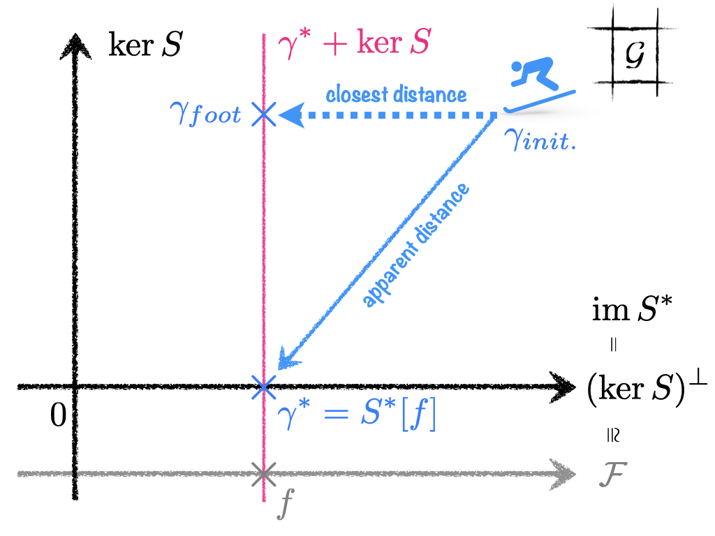
Figure 1: Orthogonal decomposition of space $\mathcal{G}$ of parameter distributions. The orthogonal projection onto abscissa, or $(\ker S)^{\perp}$, is given by $P:=S^{*}\circ S$. The range $\mathrm{im}\,S^{*}$ of the adjoint is identical to the orthocomplement $(\ker S)^{\perp}$ of the null space, and ismorphic to space $\mathcal{F}$ of functions. Note that both axes $\ker S$ and $(\ker S)^{\perp}$ are infinite-dimensional because $(\ker S)^{\perp}\cong\mathcal{F}$ and $\ker S\cong\mathcal{F}^{\mathbb{N}}$ (the structure theorem). All the distributions on the rose line $\gamma^{*}+\ker S$ indicate the same function $f$, namely, $S[\gamma^{*}+\ker S]=f$. While $\gamma^{*}=S^{*}[f]$ attains the minimum norm solution with respect to the norm $\|\cdot\|_{\mathcal{G}}$, the foot $\gamma_{foot}$ of the perpendicular line is the closest solution from the initial parameter at $\gamma_{init.}$.

Characterizing lazy learning solutions

Let us formulate lazy learning as a minimization problem of the following lazy loss:

$$J_{lazy}[\gamma]:=\|f-S[\gamma]\|_{\mathcal{F}}^{2}+\beta\|\gamma-\gamma_{init}\|_{\mathcal{G}}^{2},$$

where $\gamma_{init}$ is a given initial parameter distribution. Then, immediately because $J_{lazy}[\gamma]=J_{exp}[\gamma-\gamma_{init}]$ with the explicitly regularized loss $J_{exp}[\gamma]:=\|f-S[\gamma]\|_{\mathcal{F}}^{2}+\beta\|\gamma\|_{\mathcal{G}}^{2}$, the minimizer $\gamma_{lazy}$ of $J_{lazy}$ is given by

$$\gamma_{lazy}=S^{*}[f]+\mathrm{proj}_{\mathcal{G}\to\ker S}[\gamma_{init}]$$

as $\beta\to 0$, because the minimizer of $J_{exp}$ is given by the minimum norm solution $S^{*}[f]$ (see Sonoda et al., (2021) for example). As a result, the lazy solution $\gamma_{lazy}$ coincides with the $\gamma_{foot}$.

Improvements in generalization bounds

It has been criticized that the generalization error bounds based on the norm of parameters, or norm-based bounds (Neyshabur et al., , 2015; Bartlett et al., , 2017; Golowich et al., , 2018), tend to be extremely conservative (Zhang et al., , 2017; Nagarajan and Kolter, , 2019). On the other hand, it has also been found that those based on data-dependent (semi-)norms obtained by compressing the learned parameters, or the compression-based bounds (Arora et al., , 2018; Suzuki et al., , 2020), could provide a more realistic estimate. These findings indicate that the learned parameters obtained by deep learning are generally extremely redundant. If we suppose that some of the learned parameters only contribute to the null components, then we may understand how the norm-based bounds become extremely conservative. In fact, typical norm-based bounds regularize the norm $\|\gamma\|$ of parameter distribution $\gamma$ including the null components, while in Appendix D, we show that it is sufficient for obtaining a norm-based bound to regularize the norm $\|P[\gamma]\|$ excluding the null components. Since the null space is much larger than $\mathcal{F}$, this improvement drastically reduces the redundancy in the conventional bounds. We note that the obtained bound (Theorem 20) is not only for shallow models, but also for deep models.

Acknowledgements

This work was supported by JSPS KAKENHI 18K18113 and JST CREST JPMJCR2015.

Appendix A Further backgrounds

A.1 Overparametrization

Let us explain the background to the emergence of overparametrization in three contexts: optimization, estimation, and approximation. It was in the context of optimization that overparametrization first came to be recognized as an important factor. In spite of the fact that it is a non-convex optimization, deep learning achieves zero-training error. In the course of addressing this mystery, it was discovered that overparametrization is a sufficient condition for proving global convergence in non-convex optimization problems (Nguyen and Hein, , 2017; Chizat and Bach, , 2018; Wu et al., , 2019; Du and Hu, , 2019; Lee et al., , 2019).

In the context of estimation theory (involving statistical learning theory), it has been a great mystery that overparametrized neural networks show tremendous generalization performance on test data, because the generalization error of a typical learning model is bounded from above by $O(\sqrt{p/n})$, and thus good generalization performance cannot be expected for overparametrized models, where $n\ll p$. Therefore, instead of the parameter number $p$, several norms of the parameters are taken as a complexity $C$ of parameters that does not depend on $p$ explicitly, has been studied to obtain the generalization error bound $O(\sqrt{C/n})$ (Neyshabur et al., , 2015; Bartlett et al., , 2017; Golowich et al., , 2018). However, it has often been criticized that these norm-based bounds are still very loose, motivating a further review of generalization theory itself (Zhang et al., , 2017; Arora et al., , 2018; Nagarajan and Kolter, , 2019). Specifically, based on the fact that the regularization term is not explicitly added in typical deep learning, the idea that learning algorithms such as stochastic gradient descent (SGD) implicitly impose regularization has gained ground (Neyshabur, , 2017; Zhang et al., , 2017). In accordance with the idea of implicit regularization, two theories appeared: mean-field theory and lazy learning theory, based on the analysis of learning dynamics. Similarly, the double descent theory and benign overfitting theory have also emerged to review the idea of traditional bias-variance decomposition under overparametrization (Belkin et al., , 2019; Hastie et al., , 2019; Bartlett et al., , 2020). In Appendix D, we show that the norm-based bounds can be improved by carefully considering the null components.

On the other hand, in the context of approximation theory, infinite-width overparametrization (at $p\to\infty$) has been studied as a desirable property to simplify the analysis since the 1980s, eg., Barron’s integral representation (Barron, , 1993), Murata-Candès-Rubin’s ridgelet analysis (Murata, , 1996; Candès, , 1998; Rubin, 1998a, ) and Le Roux-Bengio’s continuous neural network (Bengio et al., , 2006). At a higher level, an integral representation can be simply defined as a $\gamma$-weighted integral $S[\gamma]({\bm{x}})=\int\gamma(\bm{v})\phi({\bm{x}},\bm{v})\mathrm{d}\bm{v}$ of a feature map $\phi({\bm{x}},\bm{v})$ parametrized by $\bm{v}$, and thus many learning machines are covered in this formulation. For example, if we assume $\gamma$ to be a probability distribution and $\phi$ to be a neuron, then it is a Bayesian neural network or a mean-field network, and if we assume $\phi$ to be a positive definite function, then it is a kernel machine. The essential benefit of the integral representation is that it transforms nonlinear maps, namely $\phi(\cdot,\bm{v})$, into linear operators, namely $S[\gamma]$. That is, the feature map $\phi$ is a nonlinear function of an original parameter $\bm{v}$, while the integral representation $S[\gamma]$ is a linear map of a distribution $\gamma$ of parameters. This linearizing effect drastically improves the perspective of theories, as already known in the theory of kernel methods. (In fact, the support vector machine was invented as a result of the functional analytic abstraction of neural networks). With the progress of overparametrization theory, the integral representation theory itself has also developed in many fields, such as the representer theorem for ReLU neural networks (Savarese et al., , 2019; Ongie et al., , 2020) and the expressive power analysis of group equivariant networks (Kumagai and Sannai, , 2020). In § 2, we develop a full set of new ridgelet analysis to involve tempered distributions $\mathcal{S}^{\prime}$ as activation function.

A.2 Basic understanding of integral representation

The integral representation is a model of a neural network composing of a single hidden layer. For each hidden parameter $({\bm{a}},b)\in\mathcal{V}$, the feature map ${\bm{x}}\mapsto\sigma({\bm{a}}\cdot{\bm{x}}-b)$ corresponds to a single neuron, and the function value $\gamma({\bm{a}},b)$ corresponds to a scalar-output parameter (weighting of the neuron).

In the integral representation, all the available neurons $\{{\bm{x}}\mapsto\sigma({\bm{a}}\cdot{\bm{x}}-b)\mid({\bm{a}},b)\in\mathcal{V}\}$ are added together. Thus, we can see that $S[\gamma]$ represents an infinitely-wide neural network, or a continuous model for short. Nonetheless, it can also represent an ordinary finite neural network, or a finite model for short, by using the Dirac measure $\delta$ on $\mathcal{V}$ to prepare a singular measure $\gamma_{p}:=\sum_{i=1}^{p}c_{i}\delta_{({\bm{a}}_{i},b_{i})}$, and plugging in it as follows:

$$S[\gamma_{p}]({\bm{x}})=\sum_{i=1}^{p}c_{i}\sigma({\bm{a}}_{i}\cdot{\bm{x}}-b_{i}),\quad{\bm{x}}\in\mathbb{R}^{m}$$ (21)

which is also equivalent to the so-called “matrix” representation such as $C\sigma(A{\bm{x}}-\bm{b})$ with matrices $A\in\mathbb{R}^{p\times m},C\in\mathbb{R}^{1\times p}$ and vector $\bm{b}\in\mathbb{R}^{p}$ followed by “element-wise” activation $\sigma$. Singular measures such as $\gamma_{p}$ can be justified without any inconsistency if we extend the class $\mathcal{G}$ of the parameter distributions to a class of Borel measures or Schwartz distributions. In the end, the integral representation can represent both continuous and finite models in the same form.

As already described, one strength of the integral representation is the so-called linearization trick. That is, while a neural network is nonlinear with respect to the naive parameter $({\bm{a}},b)$, it is linear with respect to the parameter distribution $\gamma$. This trick of embedding nonlinear objects into a linear space has been studied since the age of Frobenius, who developed the representation theory of groups. In the context of neural network study, either the integral representation by Barron, (1993) or the convex neural network by Bengio et al., (2006) are often referred.

Extension to vector-output networks is straightforward: Replacing $\gamma$ with a vector-valued one, say $\bm{\gamma}$, and acting the same operations for each component. In refappgbound, we consider vector-valued networks to deal with a function composite, namely a deep network, such as $S[\bm{\gamma}_{2}]\circ S[\bm{\gamma}_{1}]$.

A.3 How to find the ridgelet transform in a natural and inevitable manner

Historically, the ridgelet transform has been found heuristically. In the course of this study, we found that if we use the Fourier expression, then we can naturally and inevitably find the ridgelet transform as follows.

To begin with, recall that the Fourier expression of the integral representation is given by

$$S[\gamma]({\bm{x}}) :=\int_{\mathbb{R}^{m}\times\mathbb{R}}\gamma({\bm{a}},b)\sigma({\bm{a}}\cdot{\bm{x}}-b)\mathrm{d}{\bm{a}}\mathrm{d}b$$ (22)

$$=\int_{\mathbb{R}^{m}}[\gamma({\bm{a}},\cdot)*_{b}\sigma]({\bm{a}}\cdot{\bm{x}})\mathrm{d}{\bm{a}}$$ (23)

by using the identity $$\phi(b)=\frac{1}{2\pi}\int_{\mathbb{R}}\phi^{\sharp}(\omega)e^{i\omega b}\mathrm{d}\omega\,(\forall b\in\mathbb{R}) \phi(b)\leftarrow[\gamma({\bm{a}},)*_{b}\sigma](b) b\leftarrow{\bm{a}}\cdot{\bm{x}}$$ with and ,

$$=\frac{1}{2\pi}\int_{\mathbb{R}^{m}\times\mathbb{R}}\gamma^{\sharp}({\bm{a}},\omega)\sigma^{\sharp}(\omega)e^{i\omega{\bm{a}}\cdot{\bm{x}}}\mathrm{d}{\bm{a}}\mathrm{d}\omega$$ (24)

by changing the variables $$({\bm{a}},\omega)\leftarrow({\bm{a}}^{\prime}/\omega,\omega) \mathrm{d}{\bm{a}}\mathrm{d}\omega=|\omega|^{-m}\mathrm{d}{\bm{a}}^{\prime}\mathrm{d}\omega$$ with ,

$$=(2\pi)^{m-1}\int_{\mathbb{R}}\left[\frac{1}{(2\pi)^{m}}\int_{\mathbb{R}^{m}}\gamma^{\sharp}({\bm{a}}^{\prime}/\omega,\omega)e^{i{\bm{a}}^{\prime}\cdot{\bm{x}}}\mathrm{d}{\bm{a}}^{\prime}\right]\sigma^{\sharp}(\omega)|\omega|^{-m}\mathrm{d}\omega.$$ (25)

Since it contains the Fourier inversion with respect to ${\bm{a}}^{\prime}$, it is natural to consider plugging in $\gamma$ to a separation-of-variables expression as

$$\gamma^{\sharp}({\bm{a}}/\omega,\omega)\leftarrow\widehat{f}({\bm{a}})\overline{\rho^{\sharp}(\omega)},$$ (26)

with an arbitrary function $f\in L^{2}(\mathbb{R}^{m})$ and $\rho\in L_{m}^{2}(\mathbb{R})$. Then, we can see that

$$S[\gamma]({\bm{x}}) =(2\pi)^{m-1}\int_{\mathbb{R}}\left[\frac{1}{(2\pi)^{m}}\int_{\mathbb{R}^{m}}\widehat{f}({\bm{a}})e^{i{\bm{a}}\cdot{\bm{x}}}\mathrm{d}{\bm{a}}\right]\sigma^{\sharp}(\omega)\overline{\rho^{\sharp}(\omega)}|\omega|^{-m}\mathrm{d}\omega$$ (27)

$$=\langle\!\langle\sigma,\rho\rangle\!\rangle\frac{1}{(2\pi)^{m}}\int_{\mathbb{R}^{m}}\widehat{f}({\bm{a}})e^{i{\bm{a}}\cdot{\bm{x}}}\mathrm{d}{\bm{a}}\mathrm{d}\omega$$ (28)

$$=\langle\!\langle\sigma,\rho\rangle\!\rangle f({\bm{x}}).$$ (29)

Namely, we have seen that (26) provides a particular solution to the integral equation $S[\gamma]=cf$ for any given $f$ with a factor $c\in\mathbb{R}$. In fact, we can see that the RHS of (26) is (the Fourier transform of) a ridgelet transform because it is rewritten as

$$\gamma^{\sharp}({\bm{a}},\omega)=\widehat{f}(\omega{\bm{a}})\overline{\rho^{\sharp}(\omega)},$$ (30)

and thus calculated as

$$\gamma({\bm{a}},b) =\frac{1}{2\pi}\int_{\mathbb{R}}\widehat{f}(\omega{\bm{a}})\overline{\rho^{\sharp}(\omega)e^{-i\omega b}}\mathrm{d}\omega$$ (31)

$$=\frac{1}{2\pi}\int_{\mathbb{R}^{m}\times\mathbb{R}}f({\bm{x}})\overline{\rho^{\sharp}(\omega)e^{i\omega({\bm{a}}\cdot{\bm{x}}-b)}}\mathrm{d}\omega$$ (32)

$$=\int_{\mathbb{R}^{m}\times\mathbb{R}}f({\bm{x}})\overline{\rho({\bm{a}}\cdot{\bm{x}}-b)}\mathrm{d}{\bm{x}},$$ (33)

which is exactly the definition of the ridfgelet transform $R[f;\rho]$. In brief, the separation-of-variables expression (26) is the way to find the ridgelet transform.

Appendix B Theoretical Details and Proofs

In addition to $L_{m}^{2}(\mathbb{R}):=L^{2}(\mathbb{R};|\omega|^{-m}\mathrm{d}\omega)$, which is already used in the main pages, we write $L_{m}^{2}(\mathbb{R}^{m}\times\mathbb{R}):=L^{2}(\mathbb{R}^{m}\times\mathbb{R};|\omega|^{-m}\mathrm{d}{\bm{a}}\mathrm{d}\omega)$.

Remark on “$f=g$ in $L^{2}$”

An equality “$f=g$ in $L^{2}$” does not imply an equality “$f({\bm{x}})=g({\bm{x}})$ at given ${\bm{x}}$”, or the equality in the pointwise sense. By virtue of $L^{2}$-equality, we can make use of $L^{2}$-theories such as $L^{2}$-Fourier transform and $L^{2}$-inner product of functions. The ultimate goal of this study is to reveal $L^{2}$-structures of parameter distributions, such as “orthogonal decomposition,” and thus we need to employ $L^{2}$-equality.

B.1 Details on the change-of-variable $(a,\omega)\leftarrow(a/\omega,\omega)$.

To clarify the notation, we introduce an auxiliary set $U_{0}=\{({\bm{a}},\omega)\in\mathbb{R}^{m}\times\mathbb{R}\mid\omega\neq 0\}$, and a map $\varphi:\mathbb{R}^{m}\times\mathbb{R}\to\mathbb{R}^{m}\times\mathbb{R}$ defined by

$$\varphi({\bm{a}},\omega)=({\bm{a}}/\omega,\omega),\quad({\bm{a}},\omega)\in U_{0}$$ (34)

which is a continuously differentiable injection on the open set $U_{0}$. In particular, $\varphi(U_{0})=U_{0}$.

Lemma 12.

For any measurable function $\gamma:\mathbb{R}^{m}\times\mathbb{R}\to\mathbb{C}$, $\gamma\in L^{2}(\mathbb{R}^{m}\times\mathbb{R})$ if and only if $\gamma\circ\varphi\in L_{m}^{2}(\mathbb{R}^{m}\times\mathbb{R})$.

Proof.

Suppose $\gamma\in L^{2}(\mathbb{R}^{m}\times\mathbb{R})$. Since $\varphi$ is in $C^{1}(U_{0})$ and injective, change-of-variables yields

$$\int_{\varphi(U_{0})}|\gamma({\bm{a}},\omega)|^{2}\mathrm{d}{\bm{a}}\mathrm{d}\omega =\int_{U_{0}}|\gamma\circ\varphi({\bm{a}},\omega)|^{2}|\det D_{\varphi}({\bm{a}},\omega)|\mathrm{d}{\bm{a}}\mathrm{d}\omega$$ (35)

$$=\int_{U_{0}}|\gamma({\bm{a}}/\omega,\omega)|^{2}|\omega|^{-m}\mathrm{d}{\bm{a}}\mathrm{d}\omega,$$ (36)

but it yields

$$\int_{\mathbb{R}^{m}\times\mathbb{R}}|\gamma({\bm{a}},\omega)|^{2}\mathrm{d}{\bm{a}}\mathrm{d}\omega =\int_{\mathbb{R}^{m}\times\mathbb{R}}|\gamma({\bm{a}}/\omega,\omega)|^{2}|\omega|^{-m}\mathrm{d}{\bm{a}}\mathrm{d}\omega,$$ (37)

because the difference set $(\mathbb{R}^{m}\times\mathbb{R})\setminus U_{0}$ has measure-zero. Hence, we can conclude $\gamma\circ\varphi\in L_{m}^{2}(\mathbb{R})$. On the other hand, we can show the converse: If $\gamma\in L_{m}^{2}(\mathbb{R})$, then $\gamma\circ\varphi^{-1}\in L^{2}(\mathbb{R}^{m}\times\mathbb{R})$ in a similar manner. ∎

Lemma 13.

The weighted space $L_{m}^{2}(\mathbb{R}^{m}\times\mathbb{R})$ is decomposed into a topological tensor product $L^{2}(\mathbb{R}^{m})\otimes L_{m}^{2}(\mathbb{R})$.

Proof.

We write $\mathcal{G}:=L_{m}^{2}(\mathbb{R}^{m}\times\mathbb{R})$ and $\mathcal{H}:=L_{m}^{2}(\mathbb{R})$ for short. First, we can identify $\mathcal{G}$ as a vector-valued space $L^{2}(\mathbb{R}^{m};\mathcal{H})$ by identifying $\gamma\in\mathcal{G}$ as a vector-valued map $\mathbb{R}^{m}\ni{\bm{a}}\mapsto\gamma({\bm{a}},\cdot)\in\mathcal{H}$. In general, given an arbitrary measurable space $X$ and separable Hilbert space $\mathcal{H}$, a separable Hilbert space $L^{2}(X;\mathcal{H})$ can be decomposed into a topological tensor product $L^{2}(X)\otimes\mathcal{H}$ of two separable Hilbert spaces $L^{2}(X)$ and $\mathcal{H}$, namely, $L^{2}(X;\mathcal{H})=L^{2}(X)\otimes\mathcal{H}$. Therefore, we can conclude $\mathcal{G}=L^{2}(\mathbb{R}^{m};\mathcal{H})=L^{2}(\mathbb{R}^{m})\otimes\mathcal{H}$. ∎

B.2 Details on the weighted Sobolev space $H^{s}\partial^{t}(\mathbb{R}^{m}\times\mathbb{R})$

Definition 14.

For any $s,t\in\mathbb{R}$, let

$$\|\gamma\|_{H^{s}\partial^{t}}^{2}:=\int_{\mathbb{R}^{m}\times\mathbb{R}}\big{|}\langle\partial_{\omega}\rangle^{t}\left[\widecheck{\gamma}^{\sharp}(\omega{\bm{x}},\omega)\right]\big{|}^{2}\langle\omega\rangle^{2s}\mathrm{d}{\bm{x}}\mathrm{d}\omega,\quad\gamma\in\mathcal{S}^{\prime}(\mathbb{R}^{m}\times\mathbb{R}).$$ (38)

We write the corresponding Hilbert space as $H^{s}\partial^{t}(\mathbb{R}^{m}\times\mathbb{R}):=\{\gamma\in\mathcal{S}^{\prime}(\mathbb{R}^{m}\times\mathbb{R})\mid\|\gamma\|_{H^{s}\partial^{t}}<\infty\}$.

Here, the fractional operator $\langle\partial_{\omega}\rangle^{t}$ with any $t\in\mathbb{R}$ is understood as a Fourier multiplier

$$\langle\partial_{\omega}\rangle^{t}[\phi^{\sharp}(\omega)]:=\left(\langle\cdot\rangle^{t}\phi\right)^{\sharp}(\omega)=\int_{\mathbb{R}}\langle\omega\rangle^{t}\phi(\omega)e^{-i\omega\omega}\mathrm{d}\omega.$$ (39)

In particular, it satisfies

$$\int_{\mathbb{R}}\phi^{\sharp}(\omega)\overline{\langle\partial_{\omega}\rangle^{t}[\psi^{\sharp}(\omega)]}\mathrm{d}\omega=\int_{\mathbb{R}}\langle\omega\rangle^{t}\phi(\omega)\overline{\psi(\omega)}\mathrm{d}\omega=\int_{\mathbb{R}}\langle\partial_{\omega}\rangle^{t}[\phi^{\sharp}(\omega)]\overline{\psi^{\sharp}(\omega)}\mathrm{d}\omega.$$ (40)

B.3 Lemma 2

Proof.

Fix an arbitrary $\gamma\in L^{2}(\mathbb{R}^{m}\times\mathbb{R})$. Using the Plancherel formula twice, we can switch to $\widecheck{\gamma}^{\sharp}({\bm{x}},\omega)$ as below.

$$(2\pi)^{m+1}\|\gamma\|_{L^{2}(\mathbb{R}^{m}\times\mathbb{R})}^{2} =2\pi\|\widecheck{\gamma}\|_{L^{2}(\mathbb{R}^{m}\times\mathbb{R})}^{2}$$ (41)

$$=2\pi\int_{\mathbb{R}^{m}\times\mathbb{R}}|\langle b\rangle^{-t}\langle b\rangle^{t}\widecheck{\gamma}({\bm{x}},b)|^{2}\mathrm{d}{\bm{x}}\mathrm{d}b$$ (42)

since $$\langle b\rangle^{-t}\leq 1 t\geq 0$$ when ,

$$\leq 2\pi\int_{\mathbb{R}^{m}\times\mathbb{R}}|\langle b\rangle^{t}\widecheck{\gamma}({\bm{x}},b)|^{2}\mathrm{d}{\bm{x}}\mathrm{d}b$$ (43)

using the Plancherel formula,

$$=\int_{\mathbb{R}^{m}\times\mathbb{R}}|\langle\partial_{\omega}\rangle^{t}[\widecheck{\gamma}^{\sharp}({\bm{x}},\omega)]|^{2}\mathrm{d}{\bm{x}}\mathrm{d}\omega$$ (44)

letting $$({\bm{x}},\omega)\leftarrow(\omega{\bm{x}}^{\prime},\omega) \mathrm{d}{\bm{x}}\mathrm{d}\omega=|\omega|^{m}\mathrm{d}{\bm{x}}^{\prime}\mathrm{d}\omega$$ with ,

$$=\int_{\mathbb{R}^{m}\times\mathbb{R}}|\langle\partial_{\omega}\rangle^{t}[\widecheck{\gamma}^{\sharp}(\omega{\bm{x}},\omega)]|^{2}|\omega|^{m}\mathrm{d}{\bm{x}}\mathrm{d}\omega$$ (45)

since $$|\omega|^{m}\leq\langle\omega\rangle^{m}\leq\langle\omega\rangle^{2s} m\leq 2s$$ when ,

$$\leq\int_{\mathbb{R}^{m}\times\mathbb{R}}|\langle\partial_{\omega}\rangle^{t}[\widecheck{\gamma}^{\sharp}(\omega{\bm{x}},\omega)]|^{2}\langle\omega\rangle^{2s}\mathrm{d}{\bm{x}}\mathrm{d}\omega$$ (46)

$$=\|\gamma\|_{H^{s}\partial^{t}}^{2}(\mathbb{R}^{m}\times\mathbb{R}).\qed$$ (47)

B.4 Lemma 3

Fix $s,t\in\mathbb{R}$. Then, the bilinear map $S:H^{-s}\partial^{t}(\mathbb{R}^{m}\times\mathbb{R})\times\langle\cdot\rangle^{t}H^{s}(\mathbb{R})\to L^{2}(\mathbb{R}^{m})$ is bounded. Specifically,

$$\|S[\gamma]\|_{L^{2}(\mathbb{R}^{m})}\leq(2\pi)^{m-1}\|\sigma\|_{\langle\cdot\rangle^{t}H^{s}}\|\gamma\|_{H^{-s}\partial^{t}}.$$ (48)

Proof.

It is shown in Lemma 8, at (80) ∎

B.5 Lemma 7

The bilinear map $R:L^{2}(\mathbb{R}^{m})\times L_{m}^{2}(\mathbb{R})\to L^{2}(\mathbb{R}^{m}\times\mathbb{R})$ is bounded. Specifically,

$$\|R[f;\rho]\|_{L^{2}(\mathbb{R}^{m}\times\mathbb{R})}\leq(2\pi)^{m-1}\|f\|_{L^{2}(\mathbb{R}^{m})}^{2}\|\rho\|_{L_{m}^{2}(\mathbb{R})}^{2}$$ (49)

Proof.

It is shown in Lemma 8, at (64) ∎

B.6 Lemma 8

Before stepping into rigorous calculus, we present a sketch. The key step is passing to the Fourier domain via identity:

$$\phi({\bm{a}}\cdot{\bm{x}}-b)=\frac{1}{2\pi}\int_{\mathbb{R}}\phi^{\sharp}(\omega)e^{i\omega({\bm{a}}\cdot{\bm{x}}-b)}\mathrm{d}\omega,\quad({\bm{a}},b,{\bm{x}})\in\mathbb{R}^{m}\times\mathbb{R}\times\mathbb{R}^{m}.$$ (50)

We can easily check it by plugging in a number $t={\bm{a}}\cdot{\bm{x}}-b$ for the Fourier inversion formula $\phi(t)=\frac{1}{2\pi}\int_{\mathbb{R}}\phi^{\sharp}(\omega)e^{it\omega}\mathrm{d}\omega$. This is valid under a variety of assumptions on $\phi$, e.g., when $\phi\in\mathcal{S}(\mathbb{R})$.

Hence, we can rewrite the ridgelet transform as below.

$$R[f;\rho]({\bm{a}},b) =\int_{\mathbb{R}^{m}}f({\bm{x}})\overline{\rho({\bm{a}}\cdot{\bm{x}}-b)}\mathrm{d}{\bm{x}}$$ (51)

$$=\frac{1}{2\pi}\int_{\mathbb{R}^{m}\times\mathbb{R}}f({\bm{x}})\overline{\rho^{\sharp}(\omega)}e^{-i\omega({\bm{a}}\cdot{\bm{x}}-b)}\mathrm{d}\omega\mathrm{d}{\bm{x}}$$ (52)

$$=\frac{1}{2\pi}\int_{\mathbb{R}}\widehat{f}(\omega{\bm{a}})\overline{\rho^{\sharp}(\omega)}e^{i\omega b}\mathrm{d}\omega,$$ (53)

where we applied the identity (50) in the second equation, then applied a similar identity: $\int f({\bm{x}})e^{-i\omega{\bm{a}}\cdot{\bm{x}}}\mathrm{d}{\bm{x}}=\widehat{f}(\omega{\bm{a}})$ in the third equation. Finally, by taking the Fourier inversion in $b$, we have

$$R[f;\rho]^{\sharp}({\bm{a}},\omega) =\widehat{f}(\omega{\bm{a}})\overline{\rho^{\sharp}(\omega)}.$$ (54)

We note that these kind of calculus are typical in harmonic analysis involving Fourier calculus, computed tomography, and wavelet analysis.

Similarly, we can rewrite $S$ as follows:

$$S[\gamma]({\bm{x}}) =\int_{\mathbb{R}^{m}\times\mathbb{R}}\gamma({\bm{a}},b)\sigma({\bm{a}}\cdot{\bm{x}}-b)\mathrm{d}{\bm{a}}\mathrm{d}b$$ (55)

$$=\frac{1}{2\pi}\int_{\mathbb{R}^{m}\times\mathbb{R}\times\mathbb{R}}\gamma({\bm{a}},b)\sigma^{\sharp}(\omega)e^{i\omega({\bm{a}}\cdot{\bm{x}}-b)}\mathrm{d}\omega\mathrm{d}{\bm{a}}\mathrm{d}b$$ (56)

$$=\frac{1}{2\pi}\int_{\mathbb{R}^{m}\times\mathbb{R}}\gamma^{\sharp}({\bm{a}},\omega)\sigma^{\sharp}(\omega)e^{i\omega{\bm{a}}\cdot{\bm{x}}}\mathrm{d}\omega\mathrm{d}{\bm{a}},$$ (57)

where we again applied the identity (50) in the second equation, then applied an identity: $\int\gamma({\bm{a}},b)e^{-i\omega b}\mathrm{d}b=\gamma^{\sharp}({\bm{a}},\omega)$, which is simply the definition of the Fourier transform, in the third equation. In this study, we use two versions of expressions:

$$\eqref{eq:fourierS.0} =(2\pi)^{m-1}\int_{\mathbb{R}}\widecheck{\gamma}^{\sharp}(\omega{\bm{x}},\omega)\sigma^{\sharp}(\omega)\mathrm{d}\omega,$$ (58)

which is obtained by applying $(2\pi)^{-m}\int\gamma({\bm{a}},\cdot)e^{i\omega{\bm{a}}\cdot{\bm{x}}}\mathrm{d}{\bm{a}}=\widecheck{\gamma}(\omega{\bm{x}},\cdot)$; and

$$\eqref{eq:fourierS.0} =\frac{1}{2\pi}\int_{\mathbb{R}^{m}\times\mathbb{R}}\gamma^{\sharp}({\bm{a}}/\omega,\omega)\sigma^{\sharp}(\omega)|\omega|^{-m}e^{i{\bm{a}}\cdot{\bm{x}}}\mathrm{d}\omega\mathrm{d}{\bm{a}},$$ (59)

which is obtained by changing the variables $({\bm{a}},\omega)\leftarrow({\bm{a}}^{\prime}/\omega,\omega)$ with $\mathrm{d}{\bm{a}}\mathrm{d}\omega=|\omega|^{-m}\mathrm{d}{\bm{a}}^{\prime}\mathrm{d}\omega$. The second expression is convenient to make the dependence on the weight $|\omega|^{-m}$ explicit, which is a specific structure associated with the feature map ${\bm{x}}\mapsto\sigma({\bm{a}}\cdot{\bm{x}}-b)$. Finally, by taking the Fourier inversion in ${\bm{x}}$ for the second expression, we have

$$\widehat{S[\gamma]}({\bm{a}}) =(2\pi)^{m-1}\int_{\mathbb{R}}\gamma^{\sharp}({\bm{a}}/\omega,\omega)\sigma^{\sharp}(\omega)|\omega|^{-m}\mathrm{d}\omega.$$ (60)

Proof.

Here, we check that the Fourier expressions (54) and (57) hold in the sense of $L^{2}$ for the case of $\sigma\in\langle\cdot\rangle^{t}H^{s}(\mathbb{R}),\rho\in L_{m}^{2}(\mathbb{R}),\gamma\in H^{-s}\partial^{t}(\mathbb{R}^{m}\times\mathbb{R})$ and $f\in L^{2}(\mathbb{R}^{m})$.

Fourier expression of $R$

Fix an arbitary $f\in L^{2}(\mathbb{R}^{m})$ and $\rho\in L_{m}^{2}(\mathbb{R})$. We start from a function defined in a pointwise manner as

$$\gamma({\bm{a}},\omega):=\widehat{f}(\omega{\bm{a}})\overline{\rho^{\sharp}(\omega)},\quad({\bm{a}},\omega)\in\mathbb{R}^{m}\times\mathbb{R}$$ (61)

to show the equality $(2\pi)\gamma^{\sharp}=R[f;\rho]$ in the sense of $L^{2}$. First, we can verify that $\gamma\in L^{2}(\mathbb{R}^{m}\times\mathbb{R})$ because

$$\|\gamma\|_{L^{2}(\mathbb{R}^{m}\times\mathbb{R})}^{2} =\int_{\mathbb{R}^{m}\times\mathbb{R}}|\widehat{f}(\omega{\bm{a}})\overline{\rho^{\sharp}(\omega)}|^{2}\mathrm{d}{\bm{a}}\mathrm{d}\omega$$ (62)

$$=\int_{\mathbb{R}^{m}\times\mathbb{R}}|\widehat{f}({\bm{a}})\overline{\rho^{\sharp}(\omega)}|^{2}|\omega|^{-m}\mathrm{d}{\bm{a}}\mathrm{d}\omega$$ (63)

$$=(2\pi)^{m}\|f\|_{L^{2}(\mathbb{R}^{m})}^{2}\|\rho\|_{L_{m}^{2}(\mathbb{R})}^{2}<\infty,$$ (64)

where we used the Plancherel formula for $f$. Now, we can apply $L^{2}$-Fourier transform in $({\bm{a}},\omega)$ freely. Then, for any $\phi^{\sharp}\in L^{2}(\mathbb{R}^{m}\times\mathbb{R})$,

$$\langle\phi^{\sharp},\gamma\rangle_{L^{2}(\mathbb{R}^{m}\times\mathbb{R})} =\int_{\mathbb{R}^{m}\times\mathbb{R}}\overline{\phi^{\sharp}({\bm{a}},\omega)}\widehat{f}(\omega{\bm{a}})\overline{\rho^{\sharp}(\omega)}\mathrm{d}{\bm{a}}\mathrm{d}\omega$$ (65)

$$=\int_{\mathbb{R}^{m}\times\mathbb{R}}\overline{\phi^{\sharp}({\bm{a}}/\omega,\omega)}\widehat{f}({\bm{a}})\overline{\rho^{\sharp}(\omega)}|\omega|^{-m}\mathrm{d}{\bm{a}}\mathrm{d}\omega$$ (66)

$$=\int_{\mathbb{R}^{m}\times\mathbb{R}\times\mathbb{R}^{m}}\overline{\phi^{\sharp}({\bm{a}}/\omega,\omega)}f({\bm{x}})\overline{\rho^{\sharp}(\omega)}|\omega|^{-m}e^{-i{\bm{x}}\cdot{\bm{a}}}\mathrm{d}{\bm{a}}\mathrm{d}\omega\mathrm{d}{\bm{x}}$$ (67)

$$=\int_{\mathbb{R}^{m}\times\mathbb{R}\times\mathbb{R}^{m}}\overline{\phi^{\sharp}({\bm{a}},\omega)}f({\bm{x}})\overline{\rho^{\sharp}(\omega)}e^{-i\omega{\bm{x}}\cdot{\bm{a}}}\mathrm{d}{\bm{a}}\mathrm{d}\omega\mathrm{d}{\bm{x}}$$ (68)

$$=(2\pi)\int_{\mathbb{R}^{m}\times\mathbb{R}\times\mathbb{R}^{m}}\overline{\phi({\bm{a}},b)}f({\bm{x}})\overline{\rho({\bm{x}}\cdot{\bm{a}}-b)}\mathrm{d}{\bm{a}}\mathrm{d}b\mathrm{d}{\bm{x}}$$ (69)

$$=(2\pi)\langle\phi,R[f;\rho]\rangle_{L^{2}(\mathbb{R}^{m}\times\mathbb{R})}=\langle\phi^{\sharp},R[f;\rho]^{\sharp}\rangle_{L^{2}(\mathbb{R}^{m}\times\mathbb{R})}.$$ (70)

Here, we changed the variable ${\bm{a}}\leftarrow{\bm{a}}^{\prime}/\omega$ in the second equation, and changed again the variable ${\bm{a}}\leftarrow\omega{\bm{a}}^{\prime}$ in the forth equation, then applied the Plancherel formula in the fifth and seventh equations. Specifically, we can change the order of integrals freely because (67) is absolutely convergent. Namely,

$$\eqref{eq:abs conv01} \leq\|\phi({\bm{a}}/\omega,\omega)\|_{L_{m}^{2}(\mathbb{R}^{m}\times\mathbb{R})}\|f\|_{L^{2}(\mathbb{R}^{m})}\|\rho\|_{L_{m}^{2}(\mathbb{R})}.$$ (71)

Since $\langle\phi^{\sharp},\gamma\rangle=\langle\phi^{\sharp},R[f;\rho]^{\sharp}\rangle$ for any $\phi$, we can conclude $\gamma=R[f;\rho]$ in $L^{2}$.

Fourier expression of $S$

Fix $s,t\in\mathbb{R}$, $\sigma\in\langle\cdot\rangle^{t}H^{s}(\mathbb{R})$ and $\gamma\in H^{-s}\partial^{t}(\mathbb{R}^{m}\times\mathbb{R})$. We begin with (58), namely, a function defined in a pointwise manner as

$$f({\bm{x}}) :=\int_{\mathbb{R}}\widecheck{\gamma}^{\sharp}(\omega{\bm{x}},\omega)\sigma^{\sharp}(\omega)\mathrm{d}\omega,\quad{\bm{x}}\in\mathbb{R}^{m}$$ (72)

to show the equality $f=(2\pi)^{1-m}S[\gamma]$ in $L^{2}$. To be exact, the integration is understood as the action of a distribution $\sigma^{\sharp}\in\mathcal{S}^{\prime}(\mathbb{R})$. Namely,

$$f({\bm{x}})=\sigma^{\sharp}\left[\widecheck{\gamma}^{\sharp}(\cdot{\bm{x}},\cdot)\right],\quad{\bm{x}}\in\mathbb{R}^{m}.$$ (73)

First, we see that $f\in L^{2}(\mathbb{R}^{m})$. By the assumption that $\sigma\in\langle\cdot\rangle^{t}H^{s}(\mathbb{R})$, there exists $\psi\in L^{2}(\mathbb{R})$ such that $\sigma^{\sharp}(\omega)=\langle\partial_{\omega}\rangle^{t}\langle\omega\rangle^{-s}\psi^{\sharp}(\omega)$, and $\|\sigma\|_{\langle\cdot\rangle^{t}H^{s}(\mathbb{R})}=\|\psi\|_{L^{2}(\mathbb{R})}$. Hence, $f$ is rewritten as

$$f({\bm{x}}) =\int_{\mathbb{R}}\widecheck{\gamma}^{\sharp}(\omega{\bm{x}},\omega)\langle\partial_{\omega}\rangle^{t}\left[\langle\omega\rangle^{-s}\psi^{\sharp}(\omega)\right]\mathrm{d}\omega$$ (74)

$$=\int_{\mathbb{R}}\Gamma({\bm{x}},\omega)\psi^{\sharp}(\omega)\mathrm{d}\omega,$$ (75)

where we put

$$\Gamma({\bm{x}},\omega):=\langle\omega\rangle^{-s}\langle\partial_{\omega}\rangle^{t}\left[\widecheck{\gamma}^{\sharp}(\omega{\bm{x}},\omega)\right].$$ (76)

Then, the norm is bounded as

$$\|f\|_{L^{2}(\mathbb{R}^{m})}$$ (77)

$$\leq\int_{\mathbb{R}}\left(\int_{\mathbb{R}^{m}}|\Gamma({\bm{x}},\omega)|^{2}\mathrm{d}{\bm{x}}\right)^{1/2}|\psi^{\sharp}(\omega)|\mathrm{d}\omega$$ (78)

$$\leq\left(\int_{\mathbb{R}^{m}\times\mathbb{R}}|\Gamma({\bm{x}},\omega)|^{2}\mathrm{d}{\bm{x}}\mathrm{d}\omega\right)^{1/2}\left(\int_{\mathbb{R}}|\psi^{\sharp}(\omega)|^{2}\mathrm{d}\omega\right)^{1/2}$$ (79)

$$=\|\gamma\|_{H^{-s}\partial^{t}}\|\sigma\|_{\langle\cdot\rangle^{t}H^{s}}.$$ (80)

Note that since $\gamma\in L^{2}(\mathbb{R}^{m}\times\mathbb{R})$, the following equalities hold in the sense of $L^{2}$:

$$\widecheck{\gamma}^{\sharp}(\omega{\bm{x}},\omega) =(2\pi)^{-m}\int_{\mathbb{R}^{m}\times\mathbb{R}}\gamma({\bm{a}},b)e^{i\omega({\bm{a}}\cdot{\bm{x}}-b)}\mathrm{d}{\bm{a}}\mathrm{d}b$$ (81)

$$=(2\pi)^{-m}\int_{\mathbb{R}^{m}\times\mathbb{R}}\gamma({\bm{a}},{\bm{a}}\cdot{\bm{x}}-b)e^{i\omega b}\mathrm{d}{\bm{a}}\mathrm{d}b,$$ (82)

and

$$\eqref{eq:bunki} =(2\pi)^{-m}\int_{\mathbb{R}^{m}\times\mathbb{R}}\gamma({\bm{a}}/\omega,b)e^{i{\bm{a}}\cdot{\bm{x}}-i\omega b}|\omega|^{-m}\mathrm{d}{\bm{a}}\mathrm{d}b$$ (83)

$$=(2\pi)^{-m}\int_{\mathbb{R}^{m}}\gamma^{\sharp}({\bm{a}}/\omega,\omega)|\omega|^{-m}e^{i{\bm{a}}\cdot{\bm{x}}}\mathrm{d}{\bm{a}}.$$ (84)

Then, contrary to the case of $R$, we can directly calculate $f({\bm{x}})$ at any given ${\bm{x}}\in\mathbb{R}^{m}$ as follows:

$$f({\bm{x}}) =\sigma^{\sharp}\left[\widecheck{\gamma}^{\sharp}(\omega{\bm{x}},\omega)\right]$$ (85)

$$=(2\pi)^{-m}\sigma^{\sharp}\left[\int_{\mathbb{R}^{m}\times\mathbb{R}}\gamma({\bm{a}},{\bm{a}}\cdot{\bm{x}}-b)e^{i\omega b}\mathrm{d}{\bm{a}}\mathrm{d}b\right]$$ (86)

$$=(2\pi)^{1-m}\sigma\left[\int_{\mathbb{R}^{m}}\gamma({\bm{a}},{\bm{a}}\cdot{\bm{x}}-b)\mathrm{d}{\bm{a}}\right]$$ (87)

$$=(2\pi)^{1-m}\int_{\mathbb{R}}\left[\int_{\mathbb{R}^{m}}\gamma({\bm{a}},{\bm{a}}\cdot{\bm{x}}-b)\mathrm{d}{\bm{a}}\right]\sigma(b)\mathrm{d}b$$ (88)

$$=(2\pi)^{1-m}S[\gamma]({\bm{x}}),$$ (89)

where we applied the definition of Fourier transform for distributions: $\sigma^{\sharp}[\phi]:=\sigma[\phi^{\sharp}]$ for any test function $\phi$, in the forth equation. As we noted before, the second equality is in the sense of $L^{2}$. Hence, we have $f=(2\pi)^{1-m}S[\gamma]$ in $L^{2}$.

Finally, we check $\eqref{eq:fourierS.2}$. Again, for any ${\bm{x}}\in\mathbb{R}^{m}$,

$$f({\bm{x}}) =\sigma^{\sharp}\left[\widecheck{\gamma}^{\sharp}(\omega{\bm{x}},\omega)\right]$$ (90)

$$=(2\pi)^{-m}\sigma^{\sharp}\left[\int_{\mathbb{R}^{m}}\gamma^{\sharp}({\bm{a}}/\omega,\omega)|\omega|^{-m}e^{i{\bm{a}}\cdot{\bm{x}}}\mathrm{d}{\bm{a}}\right]$$ (91)

$$=(2\pi)^{-m}\int_{\mathbb{R}^{m}}\sigma^{\sharp}\left[\gamma^{\sharp}({\bm{a}}/\omega,\omega)|\omega|^{-m}\right]e^{i{\bm{a}}\cdot{\bm{x}}}\mathrm{d}{\bm{a}},$$ (92)

where the third equation is valid because $\gamma^{\sharp}({\bm{a}}/\omega,\omega)|\omega|^{-m}\in L^{2}(\mathbb{R}^{m}\times\mathbb{R})$. Therefore, by taking $L^{2}$-Fourier inversion, we have $(2\pi)^{1-m}\widehat{S[\gamma]}=\sigma^{\sharp}[\gamma^{\sharp}({\bm{a}}/\omega,\omega)|\omega|^{-m}]$ in $L^{2}$. ∎

B.7 Lemma 9

Suppose $\sigma\in\langle\cdot\rangle^{t}H^{s}(\mathbb{R})$ for some $t,s\in\mathbb{R}$. Then, the adjoint operator $S^{*}$ of $S:H^{-s}\partial^{t}(\mathbb{R}^{m}\times\mathbb{R})\to L^{2}(\mathbb{R}^{m})$ is given by $S^{*}[f]=R[f;\sigma_{*}]$ where

$$\sigma_{*}^{\sharp}(\omega):=(2\pi)^{m-1}|\omega|^{m}\langle\partial_{\omega}\rangle^{-t}\langle\omega\rangle^{2s}\langle\partial_{\omega}\rangle^{-t}\sigma^{\sharp}(\omega).$$ (93)

Specifically, it satisfies

$$\langle f,S[\gamma]\rangle_{L^{2}(\mathbb{R}^{m})} =\langle S^{*}[f],\gamma\rangle_{H^{-s}\partial^{t}}.$$ (94)

Proof.

We use the Fourier expression of $S$ given by

$$S[\gamma]({\bm{x}})=(2\pi)^{m-1}\int_{\mathbb{R}}\widecheck{\gamma}^{\sharp}(\omega{\bm{x}},\omega)\sigma^{\sharp}(\omega)\mathrm{d}\omega.$$ (95)

Then,

$$\langle f,S[\gamma]\rangle_{L^{2}(\mathbb{R}^{m})} =(2\pi)^{m-1}\int_{\mathbb{R}^{m}\times\mathbb{R}}f({\bm{x}})\overline{\widecheck{\gamma}^{\sharp}(\omega{\bm{x}},\omega)\sigma^{\sharp}(\omega)}\mathrm{d}\omega\mathrm{d}{\bm{x}}.$$ (96)

On the other hand, writing $S^{*}[f]$ as $\phi$ for brevity,

$$\langle S^{*}[f],\gamma\rangle_{H^{-s}\partial^{t}} =\int_{\mathbb{R}^{m}\times\mathbb{R}}\langle\partial_{\omega}\rangle^{t}[\widecheck{\phi}^{\sharp}(\omega{\bm{x}},\omega)]\overline{\langle\partial_{\omega}\rangle^{t}[\widecheck{\gamma}^{\sharp}(\omega{\bm{x}},\omega)]}\langle\omega\rangle^{-2s}\mathrm{d}\omega\mathrm{d}{\bm{x}}$$ (97)

$$=\int_{\mathbb{R}^{m}\times\mathbb{R}}\langle\partial_{\omega}\rangle^{t}\langle\omega\rangle^{-2s}\langle\partial_{\omega}\rangle^{t}[\widecheck{\phi}^{\sharp}(\omega{\bm{x}},\omega)]\overline{\widecheck{\gamma}^{\sharp}(\omega{\bm{x}},\omega)}\mathrm{d}\omega\mathrm{d}{\bm{x}}.$$ (98)

Hence, it suffices to take

$$\langle\partial_{\omega}\rangle^{t}\langle\omega\rangle^{-2s}\langle\partial_{\omega}\rangle^{t}[\widecheck{\phi}^{\sharp}(\omega{\bm{x}},\omega)]=(2\pi)^{m-1}f({\bm{x}})\overline{\sigma^{\sharp}(\omega)}.$$ (99)

Thus, putting $$\sigma_{*}^{\sharp}(\omega):=(2\pi)^{m-1}|\omega|^{m}\langle\partial_{\omega}\rangle^{-t}\langle\omega\rangle^{2s}\langle\partial_{\omega}\rangle^{-t}\sigma^{\sharp}(\omega) {\bm{x}}\leftarrow{\bm{x}}^{\prime}/\omega$$, and letting , we have

$$\widecheck{\phi}^{\sharp}({\bm{x}},\omega)=f({\bm{x}}/\omega)\overline{\sigma_{*}^{\sharp}(\omega)}|\omega|^{-m}.$$ (100)

By taking the Fourier transform,

$$\phi^{\sharp}({\bm{a}},\omega)=\widehat{f}(\omega{\bm{a}})\overline{\sigma_{*}^{\sharp}(\omega)}.$$ (101)

Since the RHS is a Fourier expression $R[f;\sigma_{*}]^{\sharp}({\bm{a}},\omega)$ of the ridgelet transform, we can conclude $S^{*}[f]({\bm{a}},b)=R[f;\sigma_{*}]({\bm{a}},b)$. ∎

B.8 Lemma 11

Proof.

Fix an arbitrary $\gamma\in L^{2}(\mathbb{R}^{m}\times\mathbb{R})$. Since $L^{2}$-Fourier transform is a bijection, $\gamma^{\sharp}\in L^{2}(\mathbb{R}^{m}\times\mathbb{R})$. Then, by Lemma 12, $\gamma^{\sharp}\circ\varphi\in L_{m}^{2}(\mathbb{R}^{m}\times\mathbb{R})$. Therefore, by Lemma 13, given orthonormal systems $\{\widehat{e_{i}}\}_{i\in\mathbb{N}}$ and $\{\rho^{\sharp}_{j}\}_{j\in\mathbb{N}}$ of $L^{2}(\mathbb{R}^{m})$ and $L_{m}^{2}(\mathbb{R})$ respectively, there uniquely exists an $\ell^{2}$-sequence $\{c_{ij}\}_{i,j\in\mathbb{N}}$ such that

$$\gamma^{\sharp}({\bm{a}}/\omega,\omega)=\sum_{ij}c_{ij}\widehat{e_{i}}({\bm{a}})\overline{\rho_{j}^{\sharp}(\omega)},$$ (102)

where the convergence is in $L_{m}^{2}(\mathbb{R}^{m}\times\mathbb{R})$. Specifically, the coefficients is given by

$$c_{ij} :=\int_{\mathbb{R}^{m}\times\mathbb{R}}\gamma^{\sharp}({\bm{a}}/\omega,\omega)\overline{\widehat{e_{i}}({\bm{a}})}\rho_{j}^{\sharp}(\omega)|\omega|^{-m}\mathrm{d}{\bm{a}}\mathrm{d}\omega$$ (103)

$$=\int_{\mathbb{R}^{m}\times\mathbb{R}}\gamma^{\sharp}({\bm{a}},\omega)\overline{\widehat{e_{i}}(\omega{\bm{a}})}\rho_{j}^{\sharp}(\omega)\mathrm{d}{\bm{a}}\mathrm{d}\omega$$ (104)

$$=\int_{\mathbb{R}^{m}\times\mathbb{R}}\gamma^{\sharp}({\bm{a}},\omega)\overline{R^{\sharp}[e_{i};\rho_{j}]({\bm{a}},\omega)}\mathrm{d}{\bm{a}}\mathrm{d}\omega$$ (105)

$$=(2\pi)\langle\gamma,R[e_{i};\rho_{j}]\rangle_{L^{2}(\mathbb{R}^{m}\times\mathbb{R})},$$ (106)

and satisfies

$$\sum_{ij}|c_{ij}|^{2} =\int_{\mathbb{R}^{m}\times\mathbb{R}}|\gamma^{\sharp}({\bm{a}}/\omega,\omega)|^{2}|\omega|^{-m}\mathrm{d}{\bm{a}}\mathrm{d}\omega$$ (107)

$$=\int_{\mathbb{R}^{m}\times\mathbb{R}}|\gamma^{\sharp}({\bm{a}},\omega)|^{2}\mathrm{d}{\bm{a}}\mathrm{d}\omega$$ (108)

$$=2\pi\|\gamma\|_{L^{2}(\mathbb{R}^{m}\times\mathbb{R})}^{2}.$$ (109)

By Lemma 12, the pullback $\gamma\mapsto\gamma\circ\varphi$ is bounded. Therefore, (102) yields

$$\gamma^{\sharp}({\bm{a}},\omega) =\sum_{ij}c_{ij}\widehat{e_{i}}(\omega{\bm{a}})\overline{\rho_{j}^{\sharp}(\omega)}$$ (110)

$$=\sum_{ij}c_{ij}R^{\sharp}[e_{i};\rho_{j}]({\bm{a}},\omega),$$ (111)

where the convergence is in $L^{2}(\mathbb{R}^{m}\times\mathbb{R})$. Finally, by the continuity of $L^{2}$-Fourier transform, we have

$$\gamma({\bm{a}},b)=\sum_{ij}c_{ij}R[e_{i};\rho_{j}]({\bm{a}},b),$$ (112)

where the convergence is in $L^{2}(\mathbb{R}^{m}\times\mathbb{R})$.

∎

B.9 Theorem 10

Proof.

Let $\{\widehat{e_{i}}\}_{i\in\mathbb{N}}\subset L^{2}(\mathbb{R}^{m})$ and $\{\rho^{\sharp}_{j}\}_{j\in\mathbb{N}}\subset L_{m}^{2}(\mathbb{R})$ be arbitrary orthonormal systems. Suppose $\gamma_{0}\in L^{2}(\mathbb{R}^{m}\times\mathbb{R})$ be an arbitrary null element, namely $\gamma_{0}\in\ker S$. Then, by Lemma 11, we have a unique expansion

$$\gamma_{0}=\sum_{ij}c_{ij}R[e_{i};\rho_{j}]\mbox{ in }L^{2}(\mathbb{R}^{m}\times\mathbb{R}).$$ (113)

Put

$$c^{\prime}_{i}\overline{\rho^{\prime}_{i}}:=\sum_{j}c_{ij}\overline{\rho_{j}},$$ (114)

where $\rho^{\prime}_{i}$ is normalized to $\langle\!\langle\rho^{\prime}_{i},\rho^{\prime}_{i}\rangle\!\rangle=1$ by adjusting $c^{\prime}_{i}$. Specifically, it satisfies $(c^{\prime}_{i})^{2}=\sum_{j}|c_{ij}|^{2}$ and $\sum_{i}(c^{\prime}_{i})^{2}=\|\gamma\|_{L^{2}(\mathbb{R}^{m}\times\mathbb{R})}^{2}$. It is worth noting that the obtained set $B^{\prime}:=\{\rho^{\prime}_{i}\}_{i\in\mathbb{N}}$, which may not be a basis though, is independent of the original system $B=\{\rho_{j}\}_{j\in\mathbb{N}}$ because in the Fourier expression, we can calculate $\rho^{\prime}_{i}$ as

$$c^{\prime}_{i}\overline{(\rho^{\prime}_{i})^{\sharp}(\omega)}=\sum_{j}c_{ij}\overline{\rho_{j}^{\sharp}(\omega)} =\int_{\mathbb{R}^{m}}\gamma^{\sharp}({\bm{a}}/\omega,\omega)\overline{\widehat{e_{i}}({\bm{a}})}\mathrm{d}{\bm{a}}$$ (115)

$$=(2\pi)^{-m}\int_{\mathbb{R}^{m}}\widecheck{\gamma}^{\sharp}({\bm{x}}\omega,\omega)|\omega|^{m}\overline{e_{i}({\bm{x}})}\mathrm{d}{\bm{x}}$$ (116)

$$=(2\pi)^{-m}\langle\widecheck{\gamma}^{\sharp}\circ\varphi^{-1}(\cdot,\omega),e_{i}\rangle_{L^{2}(\mathbb{R}^{m})}|\omega|^{m}.$$ (117)

By using $\rho_{i}^{\prime}$, we have another expansion

$$\gamma_{0}=\sum_{i}c^{\prime}_{i}R[e_{i};\rho^{\prime}_{i}]\mbox{ in }L^{2}(\mathbb{R}^{m}\times\mathbb{R}).$$ (118)

By the continuity of $S$, we have

$$S[\gamma_{0}]=\sum_{i}c^{\prime}_{i}S[R[e_{i};\rho^{\prime}_{i}]]=\sum_{i}c^{\prime}_{i}\langle\!\langle\sigma,\rho^{\prime}_{i}\rangle\!\rangle e_{i}=0.$$ (119)

Since $\{e_{i}\}_{i\in\mathbb{N}}$ is a basis, we have either $c^{\prime}_{i}=0$ or $\langle\!\langle\sigma,\rho^{\prime}_{i}\rangle\!\rangle=0$ for each $i\in\mathbb{N}$. But it implies the assertion.

∎

Appendix C Visualization of ridgelet spectra and reconstruction results

We present some examples of the ridgelet transforms, or the ridgelet spectra $R[f;\rho](a,b)$; and the reconstruction results $S[R[f;\rho]](x)$ for the case $\sigma(t)=\tanh t$ by using numerical integration. For visualization purposes, the data generating function is a 1-dimensional function $f(x)=\sin(2\pi x)$ for $x\in[-1,1]$. Then, the ridgelet spectrum $R[f](a,b)$ becomes a 2-dimensional function.

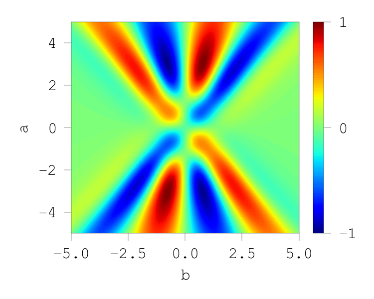
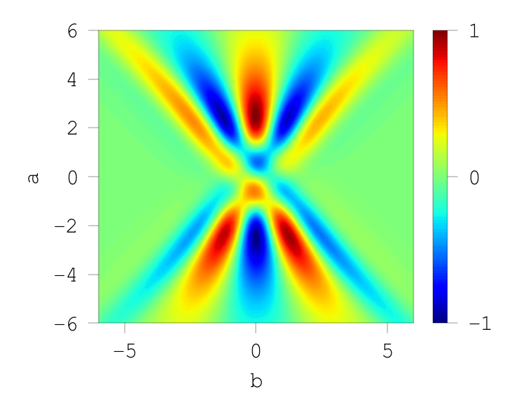
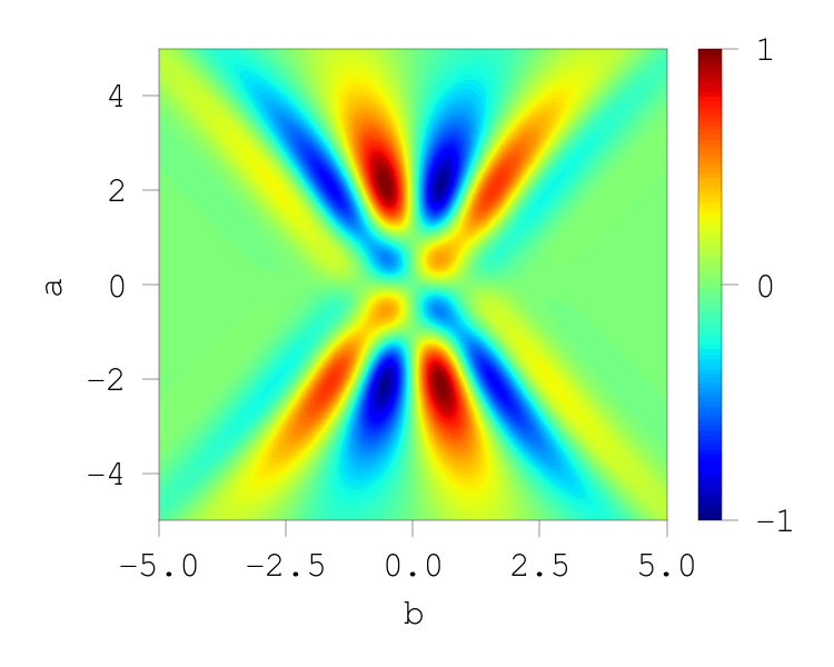
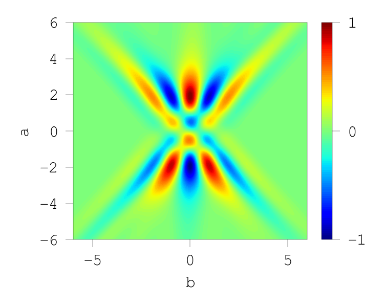
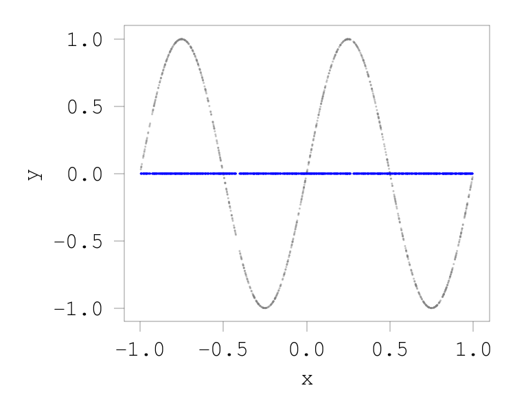
(a) $\rho_{1}$ (not a’ble)

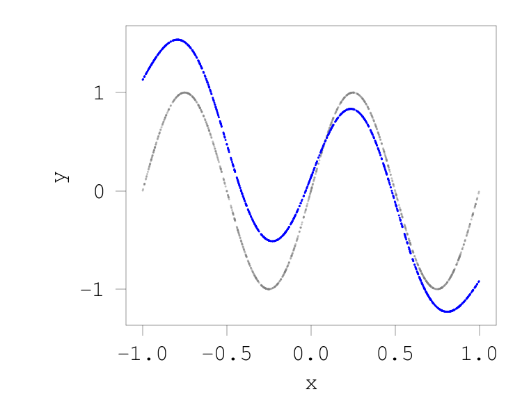
(b) $\rho_{2}$ (a’ble)

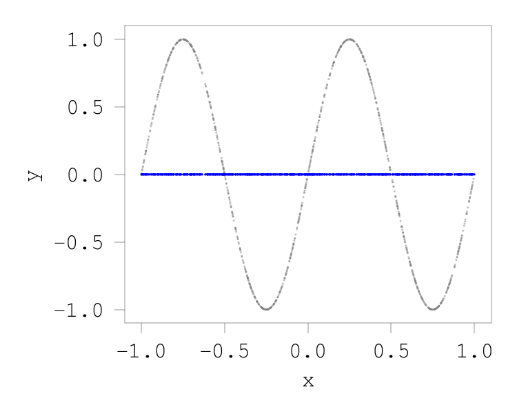
(c) $\rho_{3}$ (not a’ble)

(d) $\rho_{4}$ (a’ble)

Figure 2: Ridgelet spectra $R[f;\rho](a,b)$ (up) and reconstruction results $S[R[f;\rho]](x)$ (bottom) for $f(x)=\sin(2\pi x),x\in[-1,1]$

Construction of (non-)admissible functions

First, put the reference function as $\rho_{0}^{\sharp}(\omega):=\mathrm{sign}\,(\omega)\exp(-\omega^{2}/2)$. Here, $\rho_{0}$ is the Hilbert transform of Gaussian. In the real domain, it is a special function called the Dawson function. The Dawson function is included in several standard numerical packages for special functions, so it is easy to implement. Next, using the higher-order derivatives, set $\rho_{k}:=c_{k}\rho_{0}^{(k)}$ for $k\in\{1,2,3,4\}$. Here, $c_{k}$ are normalizing constants so that $\langle\!\langle\sigma,\rho_{k}\rangle\!\rangle=1$ (when admissible). Then, both $\rho_{2}$ and $\rho_{4}$ are admissible, while neither $\rho_{1}$ nor $\rho_{3}$ are not admissible no matter how the coefficients are set.

Proof.

The Fourier transform of $\sigma(t)=\tanh t$ is give by $\sigma^{\sharp}(\omega)=-i\pi/\sinh(\pi\omega/2)$, which is an odd function. Hence, for each $k\in\{1,2,3,4\}$, we have $(\rho_{0}^{(k)})^{\sharp}(\omega)=(i\omega)^{k}\mathrm{sign}\,(\omega)\exp(-\omega^{2}/2)$ and

$$\langle\!\langle\sigma,\rho_{k}\rangle\!\rangle =(-i)^{k}\overline{c_{k}}\int_{\mathbb{R}}\frac{\,\mathrm{sign}\,(\omega)\omega^{k-2}\exp(-\omega^{2}/2)}{\sinh(\pi\omega/2)}\mathrm{d}\omega=\begin{cases}0,&k=1,\\ \neq 0,&k=2,\\ 0,&k=3,\\ \neq 0,&k=4.\end{cases}$$ (120)

Here, the second equalities can be determined by simply checking whether the integrand is even or odd. As a result, we can see that $\rho_{2}$ and $\rho_{4}$ are admissible. On the other hand, we can see that $\rho_{1}$ and $\rho_{3}$ cannot be admissible. ∎

Details of implementation

Both $R[f](a,b)$ and $S[R[f]](x)$ were calculated by pointwise Monte Carlo integration at every sample point $(a,b)\in[-6,6]^{2}$ and $x\in[-1,1]$ resp. Namely, $R[f](a,b)\approx\frac{1}{n}\sum_{i=1}^{n}\sin(2\pi x_{i})\rho_{k}(ax_{i}-b)\Delta x$ with uniformly random $x_{i}\in[-1,1]$ and $\Delta x=1/2$; and $S[R[f]](x)\approx\frac{1}{p}\sum_{i=1}^{p}R[f](a_{i},b_{i})\sigma(a_{i}x-b_{i})\Delta a\Delta b$ with uniformly random $(a_{i},b_{i})\in[-6,6]^{2}$ and $\Delta a=\Delta b=1/12$. We used Python and especially scipy.special.dawsn for computing the Dawson function.

Visualization results

In Figure 2, we see that the ridgelet spectra (upper row) are generally signed and not compactly supported even though the data generating function $f$ is compactly supported; and that the reconstruction results (bottom row) reproduce the original function $f$ when the $\rho_{k}$ is admissible ($k=2,4$), or degenerates to zero function when the $\rho$ is not admissible ($k=1,3$). Due to numerical errors, reconstruction results contain artifacts. Nonetheless, the reconstruction results with $\rho_{1}$ and $\rho_{3}$ clearly degenerate to zero function. It is worth noting that all the four ridgelet spectra differ from each other. These differences arise from null components. In particular, the ridgelet spectra of $R[f;\rho_{1}]$ and $R[f;\rho_{3}]$ present pure nontrivial null elements.

Appendix D Improving norm-based generalization error bounds

In this section, following the conventional arguments by Golowich et al., (2018), we present an improvement of a norm-based generalization error bound in Theorem 20. (To be exact, we only provide an improved estimate of the Rademacher complexity, since it is an essential part of the generalization error bounds.)

As already mentioned, norm-based generalization error bounds, or the norm-based bounds (Neyshabur et al., , 2015; Bartlett et al., , 2017; Golowich et al., , 2018), are often loose in practice (Zhang et al., , 2017; Nagarajan and Kolter, , 2019). Using vector-valued parameter distributions $\bm{\gamma}_{i}:\mathcal{V}_{i}\to\mathbb{R}^{m_{i+1}}\,(i\in[d])$, let us consider a depth-$(d+1)$ continuous network

$$S_{d}[\bm{\gamma}_{d}]\circ\cdots\circ S_{1}[\bm{\gamma}_{1}].$$ (121)

Here, we assume that each parameter space $\mathcal{V}_{i}$ to be a subset of $\mathbb{R}^{m_{i}}\times\mathbb{R}$, so that each intermediate network becomes a vector-valued map $S_{i}[\bm{\gamma}_{i}]:\mathbb{R}^{m_{i}}\to\mathbb{R}^{m_{i+1}}$, with $m_{1}=m$ (input dimension) and $m_{d+1}=1$ (scalar output). Then, according to the conventional arguments by Golowich et al., (2018), a high-probability norm-based bound is given as follows

$$O\left(\frac{\sqrt{d}\prod_{i=1}^{d}G_{i}}{\sqrt{n}}\right).$$ (122)

(See the remarks on Theorem 20 for more details). Here, each $G_{i}$ is the upper bound of a norm $\|\bm{\gamma}_{i}\|_{L^{2}(\mathcal{V}_{i})}$ of the vector-valued parameter distribution $\bm{\gamma}_{i}$ for the $i$-th layer, and $n$ is the sample size. For a $p$-term finite vector-valued distribution $\bm{\gamma}_{i,p}:=\sum_{i=1}^{p}{\bm{c}}_{i}\delta_{({\bm{a}}_{i},b_{i})}$, the norm is attributed to the Frobenius norm $(\sum_{i=1}^{p}|{\bm{c}}_{i}|^{2})^{1/2}$. Thus, a typical norm-based generalization error bounds obtained by computing the norm of matrix parameters, such as $|C|_{F}$ and $(|A|_{F}^{2}+|b|^{2})^{1/2}$ of $C\sigma(A{\bm{x}}-{\bm{b}})$, is understood as an empirical estimate of (122). Recall here that by the structure theorem, each $\bm{\gamma}_{i}$ can be decomposed into the principal component $\bm{\gamma}_{i,\bm{f}}=S_{i}^{*}[\bm{f}_{i}]$ that can appear in the real domain as $S_{i}[\bm{\gamma}_{i,\bm{f}}]=\bm{f}_{i}$, and the null component $\bm{\gamma}_{i,0}$ that cannot appear in the real domain. In fact, by carefully reviewing the standard arguments, the upper bound $G_{i}$ of $\bm{\gamma}_{i,\bm{f}}+\bm{\gamma}_{i,0}$ can be replaced by the upper bound $G^{\prime}_{i}$ of the principal component $\bm{\gamma}_{i,\bm{f}}$ as

$$O\left(\frac{\sqrt{d}\prod_{i=1}^{d}G_{i}^{\prime}}{\sqrt{n}}\right).$$ (123)

(See Theorem 20 for more details). In other words, the conventional bound (122) obviously overestimates the error. In fact, since the null components $\bm{\gamma}_{i,0}$ are infinite-dimensional, the conventional bounds can be meaninglessly loose.

D.1 Preliminaries

Here, we recall the definition of the Rademacher complexity, and its usage for bounding the generalization error.

Definition 15 (Rademacher complexity).

Given a real-valued function class $\mathcal{H}\subset\mathbb{R}^{\mathcal{X}}$, and a set of data points ${\bm{x}}_{1:n}:=\{{\bm{x}}_{i}\}_{i=1}^{n}\subset\mathcal{X}$, the empirical Rademacher complexity is defined as

$$\widehat{\mathfrak{R}_{n}}(\mathcal{H}):=\mathbb{E}_{\epsilon_{1:n}}\left[\sup_{h\in\mathcal{H}}\frac{1}{n}\sum_{i=1}^{n}\epsilon_{i}h({\bm{x}}_{i})\right],$$ (124)

where $\epsilon_{1:n}$ is the Rademacher sequence of length $n$, or the sequence of independent uniform $\{\pm 1\}$-valued random variables. Then, the (expected) Rademacher complexity is

$$\mathfrak{R}_{n}(\mathcal{H}):=\mathbb{E}_{{\bm{x}}_{1:n}}\left[\widehat{\mathfrak{R}_{n}}(\mathcal{H})\right].$$ (125)

See Definition 2 of Bartlett and Mendelson, (2002) for more details.

Usage (Application for generalization bounds)

Theorem 16 (Mohri et al., (2018, Theorem 3.3)).

Let $\mathcal{H}$ be a class of functions $\mathcal{Z}\to[0,1]$. Then, for any $\delta>0$, with probability at least $1-\delta$ over the draw of i.i.d. sample ${\bm{z}}_{1:n}\subset\mathcal{Z}$ of size $n$, each of the following holds for all $h\in\mathcal{H}$:

$$\mathbb{E}[h({\bm{z}})] \leq\frac{1}{n}\sum_{i=1}^{n}h({\bm{z}}_{i})+2\mathfrak{R}_{n}(\mathcal{H})+\sqrt{\frac{\log(1/\delta)}{2n}},$$ (126)

$$\mathbb{E}[h({\bm{z}})] \leq\frac{1}{n}\sum_{i=1}^{n}h({\bm{z}}_{i})+2\widehat{\mathfrak{R}_{n}}(\mathcal{H})+3\sqrt{\frac{\log(2/\delta)}{2n}}.$$ (127)

Theorem 17 (Golowich et al., (2018, Theorem 4)).

Let $\mathcal{H}$ be a class of functions $\mathbb{R}^{d}\to[-R,R]$. Let $\mathcal{F}_{L,a}$ be the class of $L$-Lipschitz functions $[-R,R]\to\mathbb{R}$ satisfying $f(0)=a$. Letting $\mathcal{F}_{L,a}\circ\mathcal{H}:=\{f\circ h\mid f\in\mathcal{F}_{L,a},h\in\mathcal{H}\}$, the Rademather complexity is given by

$$\widehat{\mathfrak{R}_{n}}(\mathcal{F}_{L,a}\circ\mathcal{H})\leq cL\left(\frac{R}{\sqrt{n}}+\log^{3/2}(n)\widehat{\mathfrak{R}_{n}}(\mathcal{H})\right),$$ (128)

for some universal constant $c>0$.

D.2 Rademacher complexity for deep continuous models

Given a sequence $\{\mathcal{G}_{i}\}_{i\in[j]}$ of the spaces $\mathcal{G}_{i}$ of parameter distributions, let

$$\mathcal{H}_{j}:=\{S_{j}[\bm{\gamma}_{j}]\circ\cdots\circ S_{1}[\bm{\gamma}_{1}]\mid\bm{\gamma}_{i}\in\mathcal{G}_{i},i\in[j]\}$$ (129)

be the class of depth-$(j+1)$ vector-valued continuous networks, and with a slight abuse of notation, let $\mathcal{H}_{0}:=\{\mathrm{id}_{\mathcal{X}}\}$ be the singlet composed of the identity map on the input domain $\mathcal{X}\subset\mathbb{R}^{m}$. In the following, we use a norm

$$\|\gamma^{\prime}\|_{L^{p}(\bm{\gamma})}^{p} :=\int_{\mathcal{V}}|\gamma^{\prime}(\bm{v})|^{p}|\bm{\gamma}(\bm{v})|\mathrm{d}\bm{v},\quad p\in[1,\infty)$$ (130)

namely, a $|\bm{\gamma}|$-weighted $L^{p}$-norm.

Lemma 18 (Golowich et al., (2018, Lemma 1), modified for continuous model).

Let $\sigma$ be a 1-Lipschitz, positive-homogeneous activation function which applied element-wise (such as ReLU). Suppose that $M:=\sup_{\bm{v}\in\mathcal{V}}|\bm{v}|$ and $V:=\int_{\mathcal{V}}\mathrm{d}\bm{v}$ exist. For any class $\mathcal{H}$ of vector-valued functions on the input domain $\mathcal{X}$, any class $\mathcal{G}$ of vector-valued parameter distributions on $\mathcal{V}$ satisfying $\int_{\mathcal{V}}|\bm{\gamma}|^{2}(\bm{v})\mathrm{d}\bm{v}\leq G^{2}$ for some positive number $G$, and any convex and monotonically increasing function $g:\mathbb{R}\to\mathbb{R}_{\geq 0}$,

$$\mathbb{E}_{\epsilon_{1:n}}\left[\sup_{{\bm{h}}\in\mathcal{H},\bm{\gamma}\in\mathcal{G}}g\left(\Bigg{\|}\frac{1}{n}\sum_{i=1}^{n}\epsilon_{i}\sigma(\bm{v}\cdot{\bm{h}}({\bm{x}}_{i}))\Bigg{\|}_{L^{1}(\bm{\gamma})}\right)\right] \leq 2\mathbb{E}_{\epsilon_{1:n}}\left[\sup_{{\bm{h}}\in\mathcal{H}}g\left(MG\sqrt{V}\Bigg{|}\frac{1}{n}\sum_{i=1}^{n}\epsilon_{i}{\bm{h}}({\bm{x}}_{i})\Bigg{|}\right)\right]$$ (131)

Proof.

By Hölder’s inequality,

$$\Bigg{\|}\frac{1}{n}\sum_{i=1}^{n}\epsilon_{i}\sigma(\bm{v}\cdot{\bm{h}}({\bm{x}}_{i}))\Bigg{\|}_{L^{1}(\bm{\gamma})} :=\int_{\mathcal{V}}\Bigg{|}\frac{1}{n}\sum_{i=1}^{n}\epsilon_{i}\sigma(\bm{v}\cdot{\bm{h}}({\bm{x}}_{i}))\Bigg{|}|\bm{\gamma}|(\bm{v})\mathrm{d}\bm{v}$$ (132)

$$\leq\left(\int_{\mathcal{V}}\Bigg{|}\frac{1}{n}\sum_{i=1}^{n}\epsilon_{i}\sigma(\bm{v}\cdot{\bm{h}}({\bm{x}}_{i}))\Bigg{|}^{2}\mathrm{d}\bm{v}\right)^{1/2}\left(\int_{\mathcal{V}}|\bm{\gamma}(\bm{v})|^{2}\mathrm{d}\bm{v}\right)^{1/2}$$ (133)

$$\leq\left(\left(\int_{\mathcal{V}}\mathrm{d}\bm{v}\right)\sup_{\bm{v}\in\mathcal{V}}\Bigg{|}\frac{1}{n}\sum_{i=1}^{n}\epsilon_{i}\sigma(\bm{v}\cdot{\bm{h}}({\bm{x}}_{i}))\Bigg{|}^{2}\right)^{1/2}\left(\int_{\mathcal{V}}|\bm{\gamma}(\bm{v})|^{2}\mathrm{d}\bm{v}\right)^{1/2}$$ (134)

$$\leq G\sqrt{V}\sup_{\bm{v}\in\mathcal{V}}\Bigg{|}\frac{1}{n}\sum_{i=1}^{n}\epsilon_{i}\sigma(\bm{v}\cdot{\bm{h}}({\bm{x}}_{i}))\Bigg{|}.$$ (135)

Thus,

$$\mathbb{E}_{\epsilon_{1:n}}\left[\sup_{{\bm{h}}\in\mathcal{H},\bm{\gamma}\in\mathcal{G}}g\left(\Bigg{\|}\frac{1}{n}\sum_{i=1}^{n}\epsilon_{i}\sigma(\bm{v}\cdot{\bm{h}}({\bm{x}}_{i}))\Bigg{\|}_{L^{1}(\bm{\gamma})}\right)\right]$$ (136)

$$\leq\mathbb{E}_{\epsilon_{1:n}}\left[\sup_{h\in\mathcal{H}}g\left(G\sqrt{V}\sup_{\bm{v}\in\mathcal{V}}\Bigg{|}\frac{1}{n}\sum_{i=1}^{n}\epsilon_{i}\sigma(\bm{v}\cdot{\bm{h}}({\bm{x}}_{i}))\Bigg{|}\right)\right]$$ (137)

Since $$g(|z|)\leq g(z)+g(-z) \epsilon_{i}$$, using the symmetry of ,

$$\leq 2\mathbb{E}_{\epsilon_{1:n}}\left[\sup_{{\bm{h}}\in\mathcal{H},\bm{v}\in\mathcal{V}}g\left(G\sqrt{V}\frac{1}{n}\sum_{i=1}^{n}\epsilon_{i}\sigma(\bm{v}\cdot{\bm{h}}({\bm{x}}_{i}))\right)\right]$$ (138)

$$\leq 2\mathbb{E}_{\epsilon_{1:n}}\left[\sup_{{\bm{h}}\in\mathcal{H},\bm{v}\in\mathcal{V}}g\left(G\sqrt{V}\frac{1}{n}\sum_{i=1}^{n}\epsilon_{i}\bm{v}\cdot{\bm{h}}({\bm{x}}_{i})\right)\right]$$ (139)

$$\leq 2\mathbb{E}_{\epsilon_{1:n}}\left[\sup_{{\bm{h}}\in\mathcal{H}}g\left(MG\sqrt{V}\Bigg{|}\frac{1}{n}\sum_{i=1}^{n}\epsilon_{i}{\bm{h}}({\bm{x}}_{i})\Bigg{|}\right)\right].$$ (140)

See also Theorem 4.12 of Ledoux and Talagrand, (1991). ∎

In addition, even though we do not use the following lemma (where $\|\bm{\gamma}\|_{2}\leq G^{2}$ is replaced with $\|\bm{\gamma}\|_{1}\leq G^{p}$), if we employ it instead of the previous lemma, then we do not need the bound $V_{j}$ in Theorem 20.

Lemma 19 (Golowich et al., (2018, Lemma 1), modified for continuous model).

Let $\sigma$ be a 1-Lipschitz, positive-homogeneous activation function which applied element-wise (such as ReLU). Suppose that $M:=\sup_{\bm{v}\in\mathcal{V}}|\bm{v}|$ exists. For any class $\mathcal{H}$ of vector-valued functions on $\mathcal{X}$, any class $\mathcal{G}$ of vector-valued parameter distributions on $\mathcal{V}$ satisfying $\int_{\mathcal{V}}|\gamma|(\bm{v})\mathrm{d}\bm{v}\leq G^{p}$ for some positive number $G$, and any convex and monotonically increasing function $g:\mathbb{R}\to\mathbb{R}_{\geq 0}$,

$$\mathbb{E}_{\epsilon_{1:n}}\left[\sup_{{\bm{h}}\in\mathcal{H},\bm{\gamma}\in\mathcal{G}}g\left(\Bigg{\|}\frac{1}{n}\sum_{i=1}^{n}\epsilon_{i}\sigma(\bm{v}\cdot{\bm{h}}({\bm{x}}_{i}))\Bigg{\|}_{L^{p}(\bm{\gamma})}\right)\right] \leq 2\mathbb{E}_{\epsilon_{1:n}}\left[\sup_{{\bm{h}}\in\mathcal{H}}g\left(MG\Bigg{|}\frac{1}{n}\sum_{i=1}^{n}\epsilon_{i}{\bm{h}}({\bm{x}}_{i})\Bigg{|}\right)\right]$$ (141)

Proof.

By Hölder’s inequality,

$$\Bigg{\|}\frac{1}{n}\sum_{i=1}^{n}\epsilon_{i}\sigma(\bm{v}\cdot{\bm{h}}({\bm{x}}_{i}))\Bigg{\|}_{L^{p}(\bm{\gamma})}^{p} :=\int_{\mathcal{V}}\Bigg{|}\frac{1}{n}\sum_{i=1}^{n}\epsilon_{i}\sigma(\bm{v}\cdot{\bm{h}}({\bm{x}}_{i}))\Bigg{|}^{p}|\bm{\gamma}|(\bm{v})\mathrm{d}\bm{v}$$ (142)

$$\leq G^{p}\sup_{\bm{v}\in\mathcal{V}}\Bigg{|}\frac{1}{n}\sum_{i=1}^{n}\epsilon_{i}\sigma(\bm{v}\cdot{\bm{h}}({\bm{x}}_{i}))\Bigg{|}^{p}.$$ (143)

Thus,

$$\mathbb{E}_{\epsilon_{1:n}}\left[\sup_{{\bm{h}}\in\mathcal{H},\bm{\gamma}\in\mathcal{G}}g\left(\Bigg{\|}\frac{1}{n}\sum_{i=1}^{n}\epsilon_{i}\sigma(\bm{v}\cdot{\bm{h}}({\bm{x}}_{i}))\Bigg{\|}_{L^{p}(\bm{\gamma})}\right)\right]$$ (144)

$$\leq\mathbb{E}_{\epsilon_{1:n}}\left[\sup_{h\in\mathcal{H},\bm{v}\in\mathcal{V}}g\left(G\Bigg{|}\frac{1}{n}\sum_{i=1}^{n}\epsilon_{i}\sigma(\bm{v}\cdot{\bm{h}}({\bm{x}}_{i}))\Bigg{|}\right)\right]$$ (145)

Since $$g(|z|)\leq g(z)+g(-z) \epsilon_{i}$$, using the symmetry of ,

$$\leq 2\mathbb{E}_{\epsilon_{1:n}}\left[\sup_{{\bm{h}}\in\mathcal{H},\bm{v}\in\mathcal{V}}g\left(G\frac{1}{n}\sum_{i=1}^{n}\epsilon_{i}\sigma(\bm{v}\cdot{\bm{h}}({\bm{x}}_{i}))\right)\right]$$ (146)

By the $$1$$-Lipschitz continuity and using Ledoux and Talagrand, (1991, Theorem 4.12),

$$\leq 2\mathbb{E}_{\epsilon_{1:n}}\left[\sup_{{\bm{h}}\in\mathcal{H},\bm{v}\in\mathcal{V}}g\left(G\frac{1}{n}\sum_{i=1}^{n}\epsilon_{i}\bm{v}\cdot{\bm{h}}({\bm{x}}_{i})\right)\right]$$ (147)

$$\leq 2\mathbb{E}_{\epsilon_{1:n}}\left[\sup_{{\bm{h}}\in\mathcal{H}}g\left(MG\Bigg{|}\frac{1}{n}\sum_{i=1}^{n}\epsilon_{i}{\bm{h}}({\bm{x}}_{i})\Bigg{|}\right)\right]\qed$$ (148)

Theorem 20 (Golowich et al., (2018, Theorem 1), modified for continuous model).

Let $\mathcal{H}_{d}$ be the class of real-valued networks of depth-$(d+1)$ over a bounded domain $\mathcal{X}\subset\{{\bm{x}}\in\mathbb{R}^{m}\mid|{\bm{x}}|\leq B\}$. Suppose that the activation functions satisfy the assumptions in Lemma 18; and suppose that each parameter distribution $\bm{\gamma}_{j}\in\mathcal{G}_{j}$ is uniformly restricted to $\int_{\mathcal{V}_{j}}|P_{j}[\bm{\gamma}_{j}](\bm{v})|^{2}\mathrm{d}\bm{v}\leq G_{j}^{2}$ with some universal constant $G_{j}>0$ by using the orthogonal projection $P_{j}=S_{j}^{*}\circ S_{j}$ onto $(\ker S_{j})^{\perp}$, and that it is supported in a bounded domain $\mathcal{V}_{j}\subset\{\bm{v}\in\mathbb{R}^{h_{j}}\mid|\bm{v}|\leq M_{j}\}$ with volume $V_{j}:=\int_{\mathcal{V}_{j}}\mathrm{d}\bm{v}$. Then, the Rademacher complexity is estimated as

$$\widehat{\mathfrak{R}_{n}}(\mathcal{H}_{d})\leq\frac{B(\sqrt{2d\log 2}+1)\prod_{j=1}^{d}M_{j}\sqrt{V_{j}}G_{j}}{\sqrt{n}}.$$ (149)

Proof.

Fix $t>0$ to be chosen later. Then, the Rademacher complexity of $\mathcal{H}_{j}$ can be upper bounded as follows:

$$\widehat{\mathfrak{R}_{n}}(\mathcal{H}_{j}) =\mathbb{E}_{\epsilon_{1:n}}\left[\sup_{\gamma\in\mathcal{G}_{j},{\bm{h}}\in\mathcal{H}_{j-1}}\frac{1}{n}\sum_{i=1}^{n}\epsilon_{i}S_{j}[P_{j}[\bm{\gamma}]]({\bm{h}}({\bm{x}}_{i}))\right]$$ (150)

$$=\frac{1}{t}\log\circ\exp\left(\mathbb{E}_{\epsilon_{1:n}}\left[\sup_{\gamma\in\mathcal{G}_{j},{\bm{h}}\in\mathcal{H}_{j-1}}\frac{t}{n}\sum_{i=1}^{n}\epsilon_{i}S_{j}[P_{j}[\bm{\gamma}]]({\bm{h}}({\bm{x}}_{i}))\right]\right)$$ (151)

By Jensen’s inequality,

$$\leq\frac{1}{t}\log\left(\mathbb{E}_{\epsilon_{1:n}}\left[\sup_{\gamma\in\mathcal{G}_{j},{\bm{h}}\in\mathcal{H}_{j-1}}\exp\left(\frac{t}{n}\sum_{i=1}^{n}\epsilon_{i}S_{j}[P_{j}[\bm{\gamma}]]({\bm{h}}({\bm{x}}_{i}))\right)\right]\right)$$ (152)

$$=\frac{1}{t}\log\left(\mathbb{E}_{\epsilon_{1:n}}\left[\sup_{\gamma\in\mathcal{G}_{j},{\bm{h}}\in\mathcal{H}_{j-1}}\exp\left(\int_{\mathcal{V}}\frac{t}{n}\sum_{i=1}^{n}\epsilon_{i}\sigma(\bm{v}\cdot{\bm{h}}({\bm{x}}_{i}))P_{j}[\bm{\gamma}](\bm{v})\mathrm{d}\bm{v}\right)\right]\right)$$ (153)

$$\leq\frac{1}{t}\log\left(\mathbb{E}_{\epsilon_{1:n}}\left[\sup_{\gamma\in\mathcal{G}_{j},{\bm{h}}\in\mathcal{H}_{j-1}}\exp\left(t\int_{\mathcal{V}}\Bigg{|}\frac{1}{n}\sum_{i=1}^{n}\epsilon_{i}\sigma(\bm{v}\cdot{\bm{h}}({\bm{x}}_{i}))\Bigg{|}|P_{j}[\bm{\gamma}](\bm{v})|\mathrm{d}\bm{v}\right)\right]\right)$$ (154)

$$=\frac{1}{t}\log\left(\mathbb{E}_{\epsilon_{1:n}}\left[\sup_{\gamma\in\mathcal{G}_{j},{\bm{h}}\in\mathcal{H}_{j-1}}\exp\left(t\Bigg{\|}\frac{1}{n}\sum_{i=1}^{n}\epsilon_{i}\sigma(\bm{v}\cdot{\bm{h}}({\bm{x}}_{i}))\Bigg{\|}_{L^{1}(P_{j}[\bm{\gamma}])}\right)\right]\right)$$ (155)

By Lemma 18,

$$\leq\frac{1}{t}\log\left(2\mathbb{E}_{\epsilon_{1:n}}\left[\sup_{{\bm{h}}\in\mathcal{H}_{j-1}}\exp\left(tM_{j}G_{j}\sqrt{V_{j}}\Bigg{|}\frac{1}{n}\sum_{i=1}^{n}\epsilon_{i}{\bm{h}}({\bm{x}}_{i})\Bigg{|}\right)\right]\right)$$ (156)

Hence, letting ${\bm{h}}=S_{j-1}[\bm{\gamma}]\circ{\bm{h}}^{\prime}$ and repeating the process from $j=d$ to $1$, we have

$$\widehat{\mathfrak{R}_{n}}(\mathcal{H}_{d}) \leq\frac{1}{t}\log\left(2^{d}\mathbb{E}_{\epsilon_{1:n}}\left[\exp\left(tC\Bigg{|}\frac{1}{n}\sum_{i=1}^{n}\epsilon_{i}{\bm{x}}_{i}\Bigg{|}\right)\right]\right),$$ (157)

where we put $C:=\prod_{j=1}^{d}M_{j}\sqrt{V_{j}}G_{j}$. (Following the same arguments with Theorem 1, Golowich et al., (2018) to conclude the claim.) ∎

Remark

By using $S_{j}[P_{j}[\bm{\gamma}]]=S_{j}[\bm{\gamma}]$, we can replace the exclusive norm $\|P_{j}[\bm{\gamma}_{j}]\|_{L^{2}(\mathcal{V}_{j})}=\|\bm{\gamma}_{j,\bm{f}}\|_{L^{2}(\mathcal{V}_{j})}$ in the proof with the inclusive norm $\|\bm{\gamma}_{j}\|_{L^{2}(\mathcal{V}_{j})}=\|\bm{\gamma}_{j,\bm{f}}+\bm{\gamma}_{j,0}\|_{L^{2}(\mathcal{V}_{j})}$, leading to the conventional (loose) bound as shown in (122).