\forLoop

126calBbCounter

Submodular + Concave
 

Siddharth Mitra
Yale University
siddharth.mitra@yale.edu
   Moran Feldman
University of Haifa
moranfe@cs.haifa.ac.il
   Amin Karbasi
Yale University
amin.karbasi@yale.edu
Abstract

It has been well established that first order optimization methods can converge to the maximal objective value of concave functions and provide constant factor approximation guarantees for (non-convex/non-concave) continuous submodular functions. In this work, we initiate the study of the maximization of functions of the form F(x)=G(x)+C(x)𝐹𝑥𝐺𝑥𝐶𝑥F(x)=G(x)+C(x) over a solvable convex body P𝑃P, where G𝐺G is a smooth DR-submodular function and C𝐶C is a smooth concave function. This class of functions is a strict extension of both concave and continuous DR-submodular functions for which no theoretical guarantee is known. We provide a suite of Frank-Wolfe style algorithms, which, depending on the nature of the objective function (i.e., if G𝐺G and C𝐶C are monotone or not, and non-negative or not) and on the nature of the set P𝑃P (i.e., whether it is downward closed or not), provide 11/e11𝑒1-1/e, 1/e1𝑒1/e, or 1/2121/2 approximation guarantees. We then use our algorithms to get a framework to smoothly interpolate between choosing a diverse set of elements from a given ground set (corresponding to the mode of a determinantal point process) and choosing a clustered set of elements (corresponding to the maxima of a suitable concave function). Additionally, we apply our algorithms to various functions in the above class (DR-submodular + concave) in both constrained and unconstrained settings, and show that our algorithms consistently outperform natural baselines.

1 Introduction

Despite their simplicity, first-order optimization methods (such as gradient descent and its variants, Frank-Wolfe, momentum based methods, and others) have shown great success in many machine learning applications. A large body of research in the operations research and machine learning communities has fully demystified the convergence rate of such methods in minimizing well behaved convex objectives (Bubeck, 2015; Nesterov, 2018). More recently, a new surge of rigorous results has also shown that gradient descent methods can find the global minima of specific non-convex objective functions arisen from non-negative matrix factorization (Arora et al., 2012), robust PCA (Netrapalli et al., 2014), phase retrieval (Chen et al., 2019b), matrix completion (Sun and Luo, 2016), and the training of wide neural networks (Du et al., 2019; Jacot et al., 2018; Allen-Zhu et al., 2019), to name a few. It is also very well known that finding the global minimum of a general non-convex function is indeed computationally intractable (Murty and Kabadi, 1987). To avoid such impossibility results, simpler goals have been pursued by the community: either developing algorithms that can escape saddle points and reach local minima (Ge et al., 2015) or describing structural properties which guarantee that reaching a local minimizer ensures optimality (Sun et al., 2016; Bian et al., 2017b; Hazan et al., 2016). In the same spirit, this paper quantifies a large class of non-convex functions for which first-order optimization methods provably achieve near optimal solutions.

More specifically, we consider objective functions that are formed by the sum of a continuous DR-submodular function G(x)𝐺𝑥G(x) and a concave function C(x)𝐶𝑥C(x). Recent research in non-convex optimization has shown that first-order optimization methods provide constant factor approximation guarantees for maximizing continuous submodular functions Bian et al. (2017b); Hassani et al. (2017); Bian et al. (2017a); Niazadeh et al. (2018); Hassani et al. (2020a); Mokhtari et al. (2018a). Similarly, such methods find the global maximizer of concave functions. However, the class of F(x)=G(x)+C(x)𝐹𝑥𝐺𝑥𝐶𝑥F(x)=G(x)+C(x) functions is strictly larger than both concave and continuous DR-submodular functions. More specifically, F(x)𝐹𝑥F(x) is not concave nor continuous DR-submodular in general (Figure 1 illustrates an example). In this paper, we show that first-order methods provably provide strong theoretical guarantees for maximizing such functions.

The combinations of continuous submodular and concave functions naturally arise in many ML applications such as maximizing a regularized submodular function (Kazemi et al., 2020a) or finding the mode of distributions (Kazemi et al., 2020a; Robinson et al., 2019). For instance, it is common to add a regularizer to a D-optimal design objective function to increase the stability of the final solution against perturbations (He, 2010; Derezinski et al., 2020; Lattimore and Szepesvari, 2020). Similarly, many instances of log-submodular distributions, such as determinantal point processes (DPPs), have been studied in depth in order to sample a diverse set of items from a ground set (Kulesza, 2012; Rebeschini and Karbasi, 2015; Anari et al., 2016). In order to control the level of diversity, one natural recipe is to consider the combination of a log-concave (e.g., normal distribution, exponential distribution and Laplace distribution) (Dwivedi et al., 2019; Robinson et al., 2019) and log-submodular distributions (Djolonga and Krause, 2014; Bresler et al., 2019), i.e., Pr(\vx)exp(λC(\vx)+(1λ)G(\vx))proportional-toPr\vx𝜆𝐶\vx1𝜆𝐺\vx\Pr(\vx)\propto\exp(\lambda C(\vx)+(1-\lambda)G(\vx)) for some λ[0,1]𝜆01\lambda\in[0,1]. In this way, we can obtain a class of distributions that contains log-concave and log-submodular distributions as special cases. However, this class of distributions is strictly more expressive than both log-concave and log-submodular models, e.g., in contrast to log-concave distributions, they are not uni-modal in general. Finding the mode of such distributions amounts to maximizing a combination of a continuous DR-submodular function and a concave function. The contributions of this paper are as follows.

  • Assuming first-order oracle access for the function F𝐹F, we develop the algorithms: Greedy Frank-Wolfe (Algorithm 1) and Measured Greedy Frank-Wolfe (Algorithm 2) which achieve constant factors approximation guarantees between 11/e11𝑒1-1/e and 1/e1𝑒1/e depending on the setting, i.e. depending on the monotonicity and non-negativity of G𝐺G and C𝐶C, and depending on the constraint set having the down-closeness property or not.

  • Furthermore, if we have access to the individual gradients of G𝐺G and C𝐶C, then we are able to make the guarantee with respect to C𝐶C exact using the algorithms: Gradient Combining Frank-wolfe (Algorithm 3) and Non-oblivious Frank-Wolfe (Algorithm 4). These results are summarized and made more precise in Table 1 and Section 3.

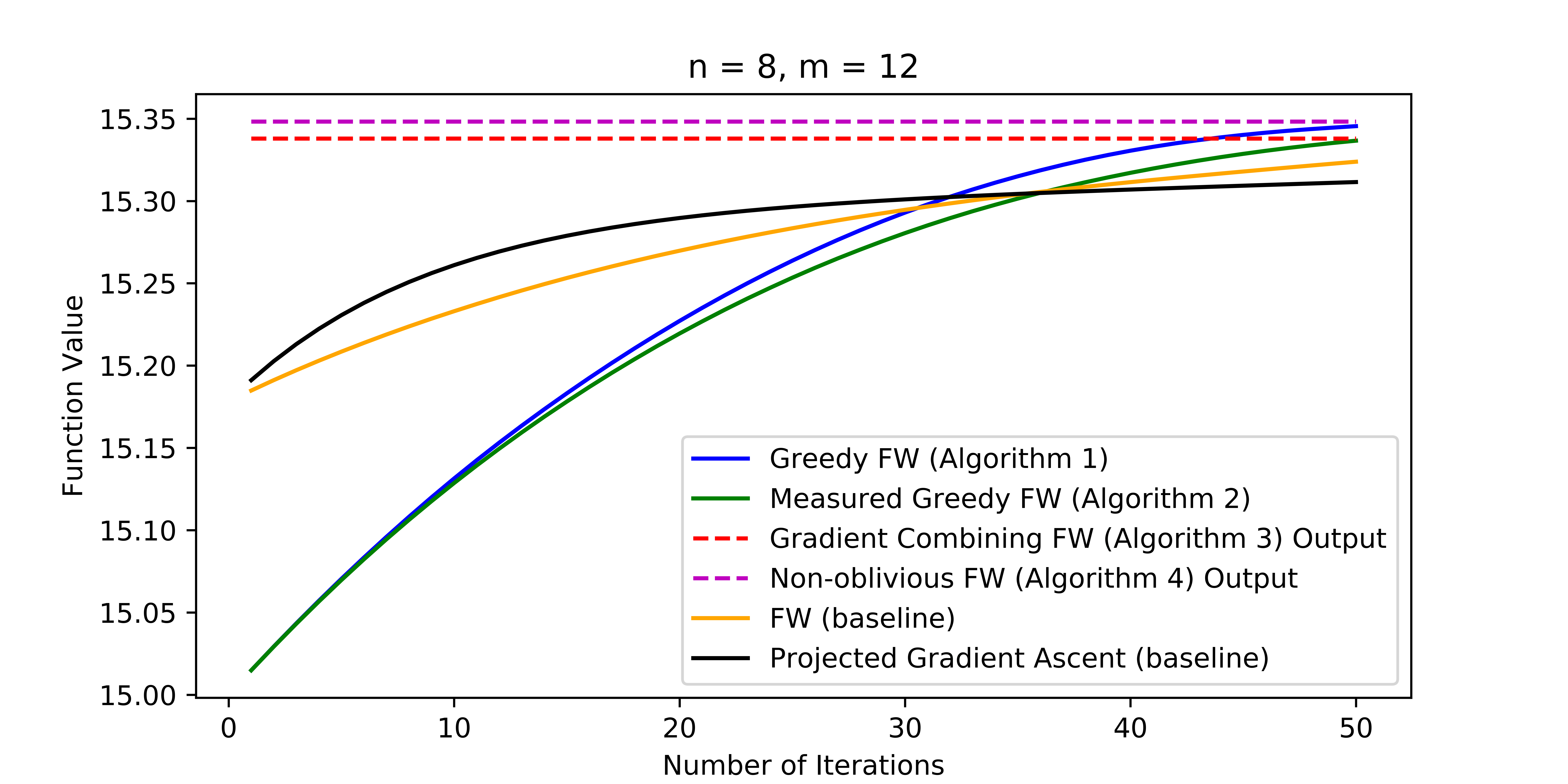
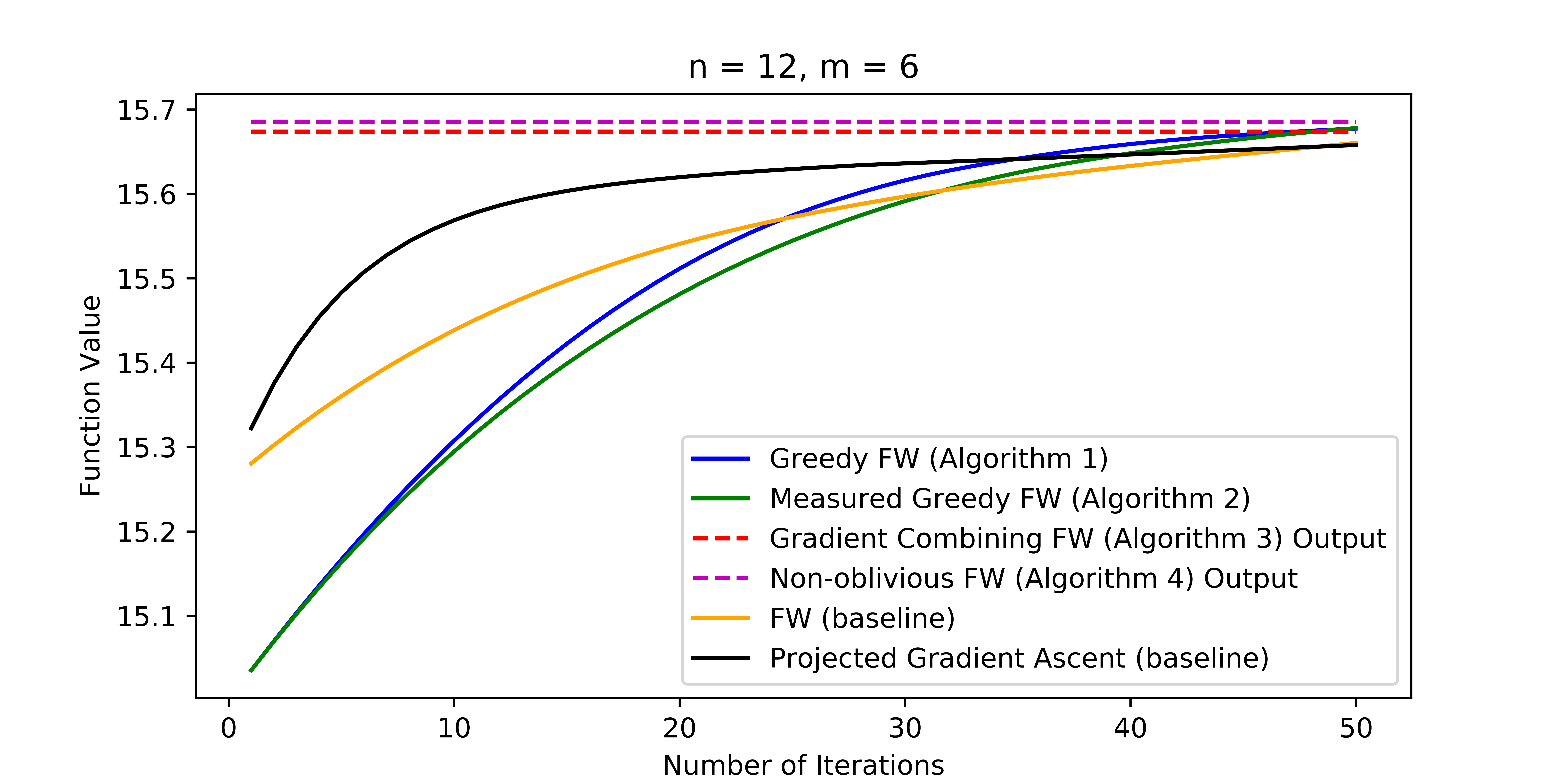
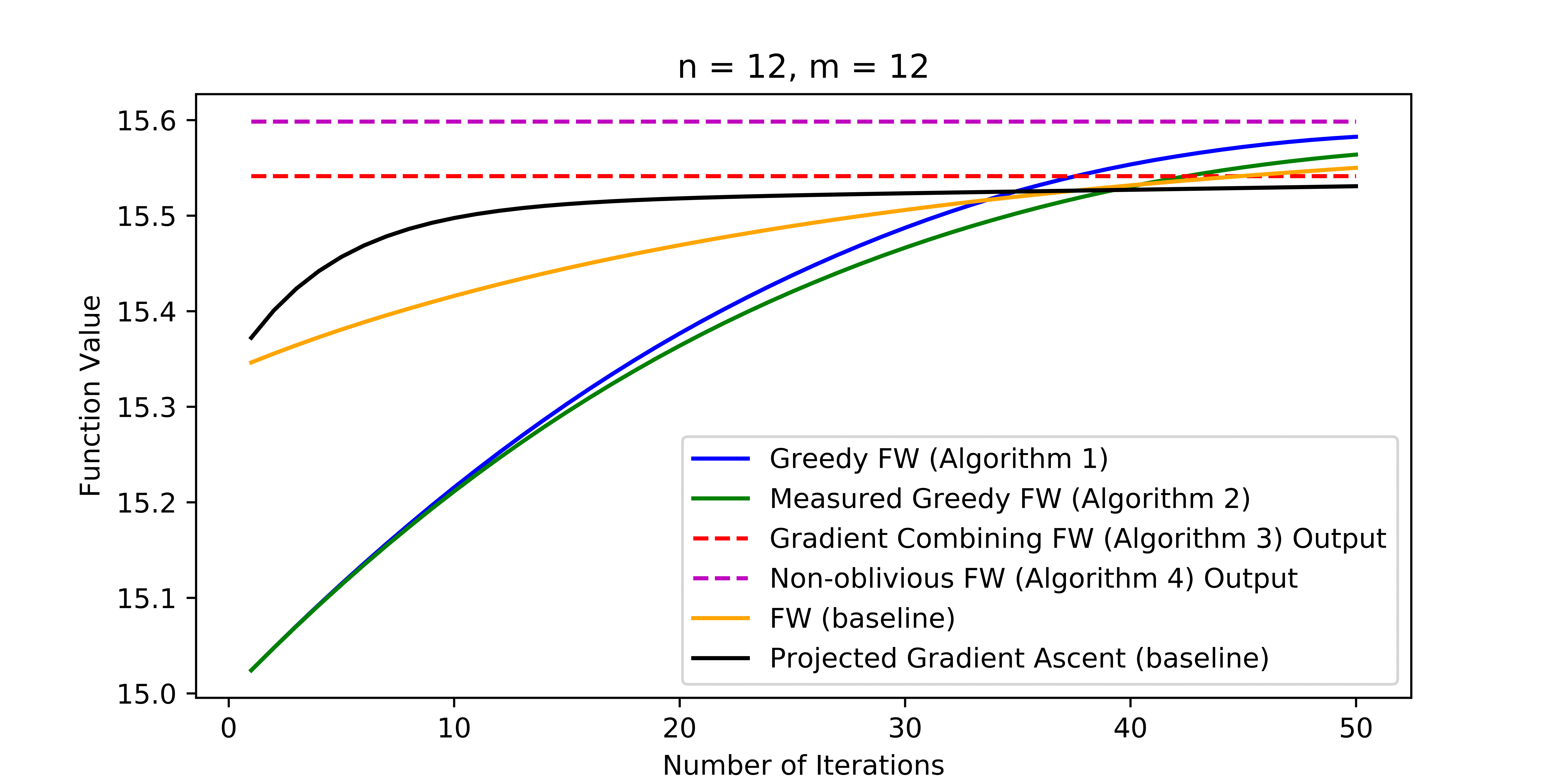
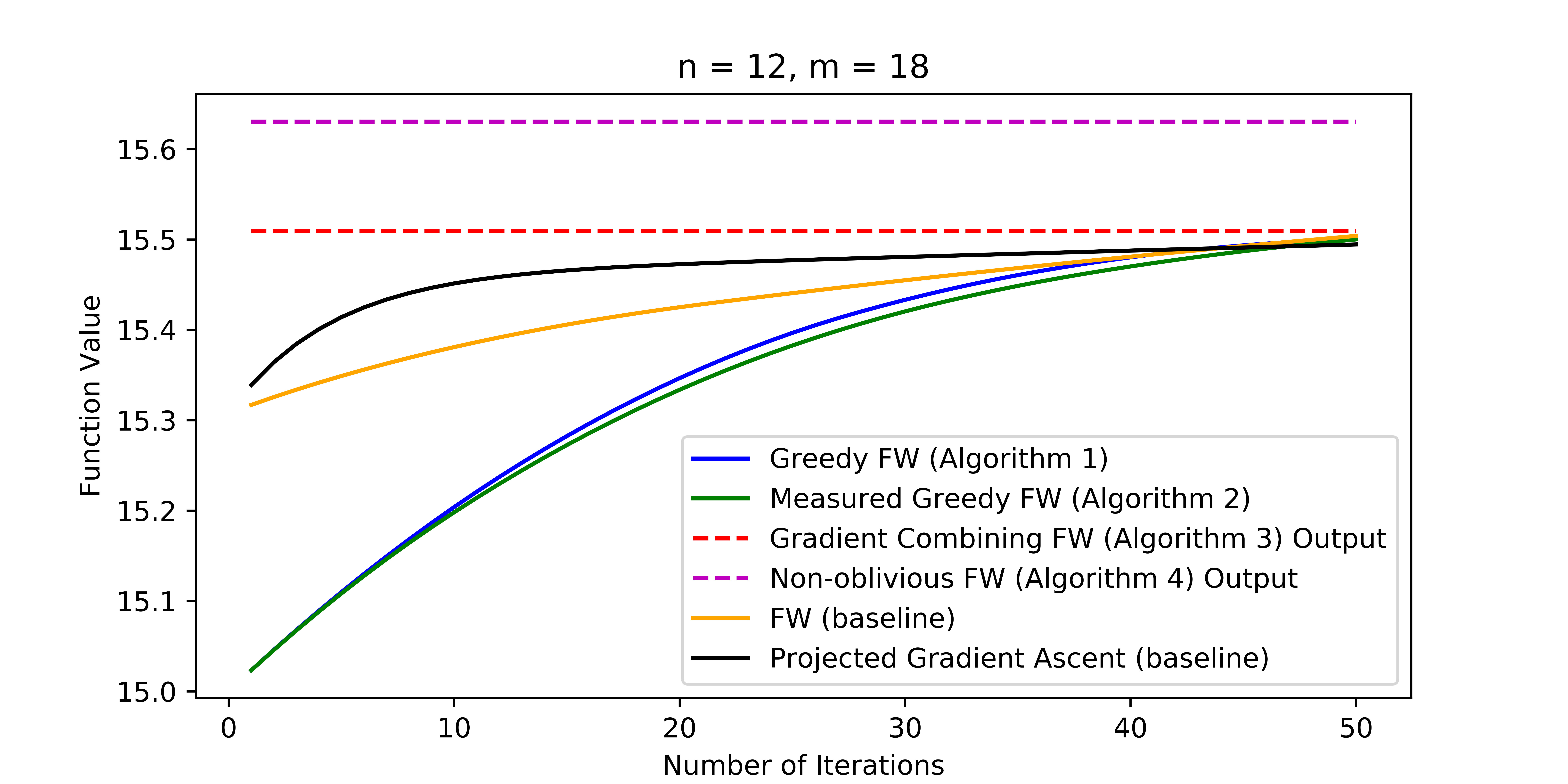
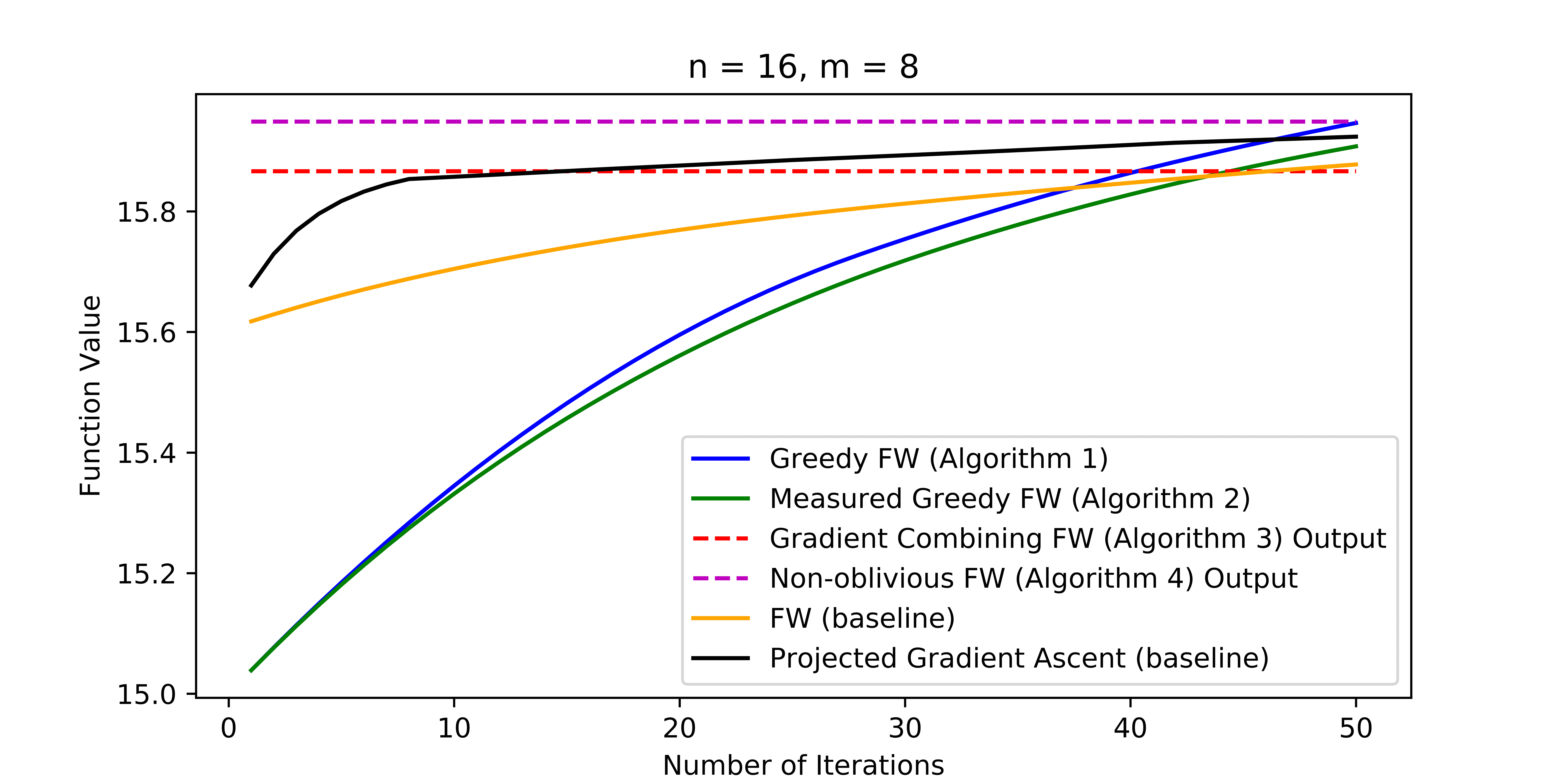
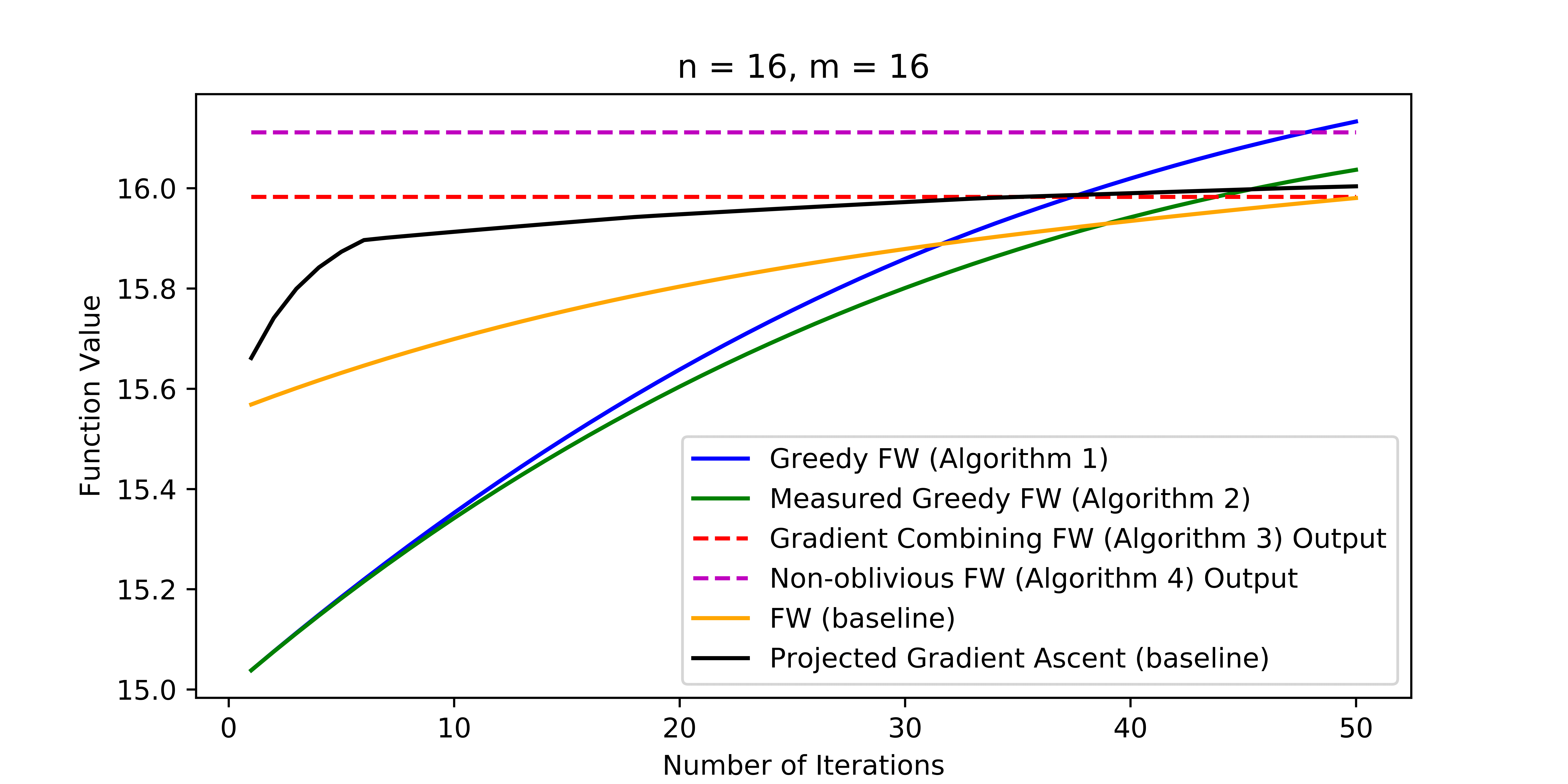
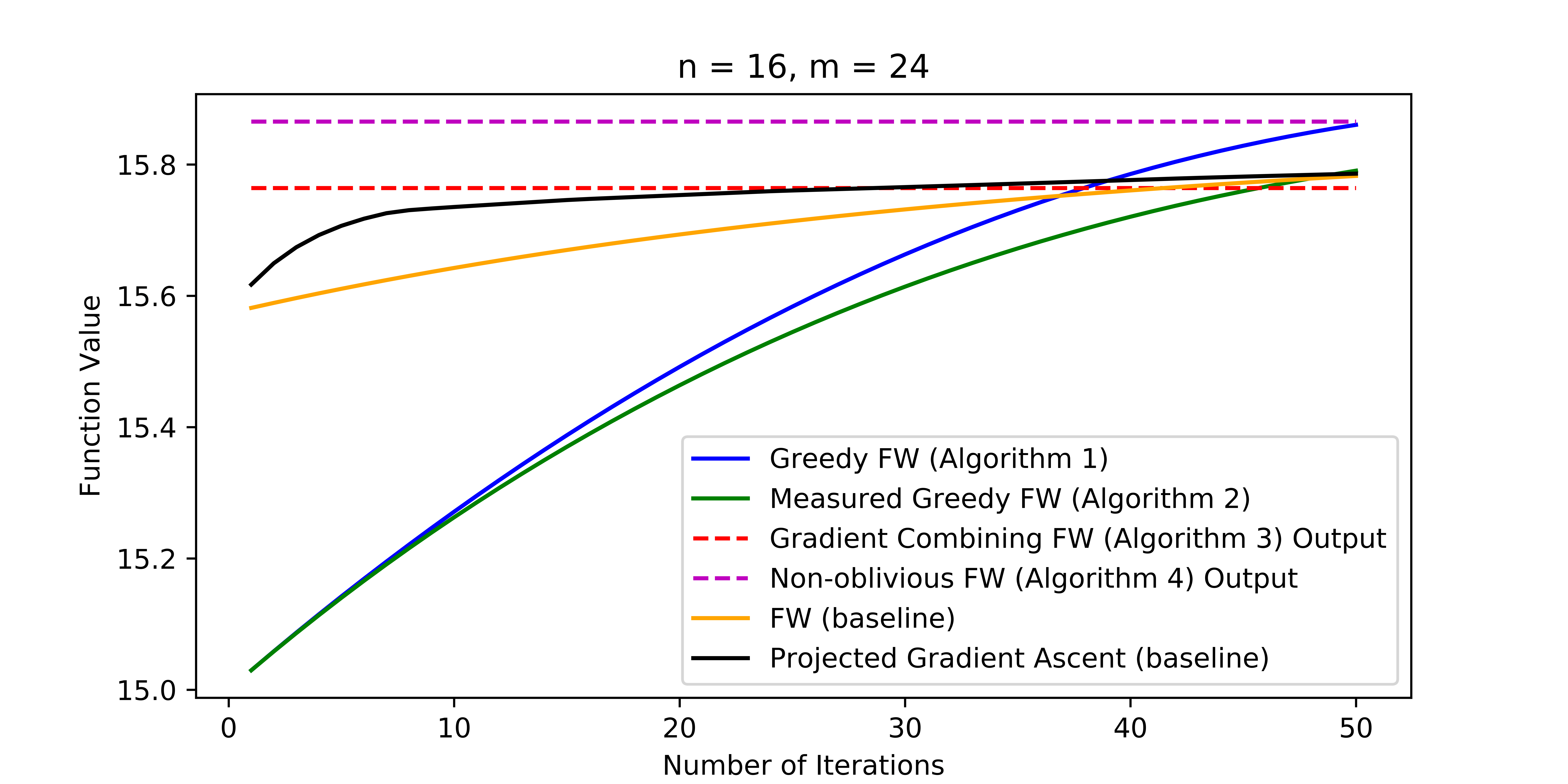
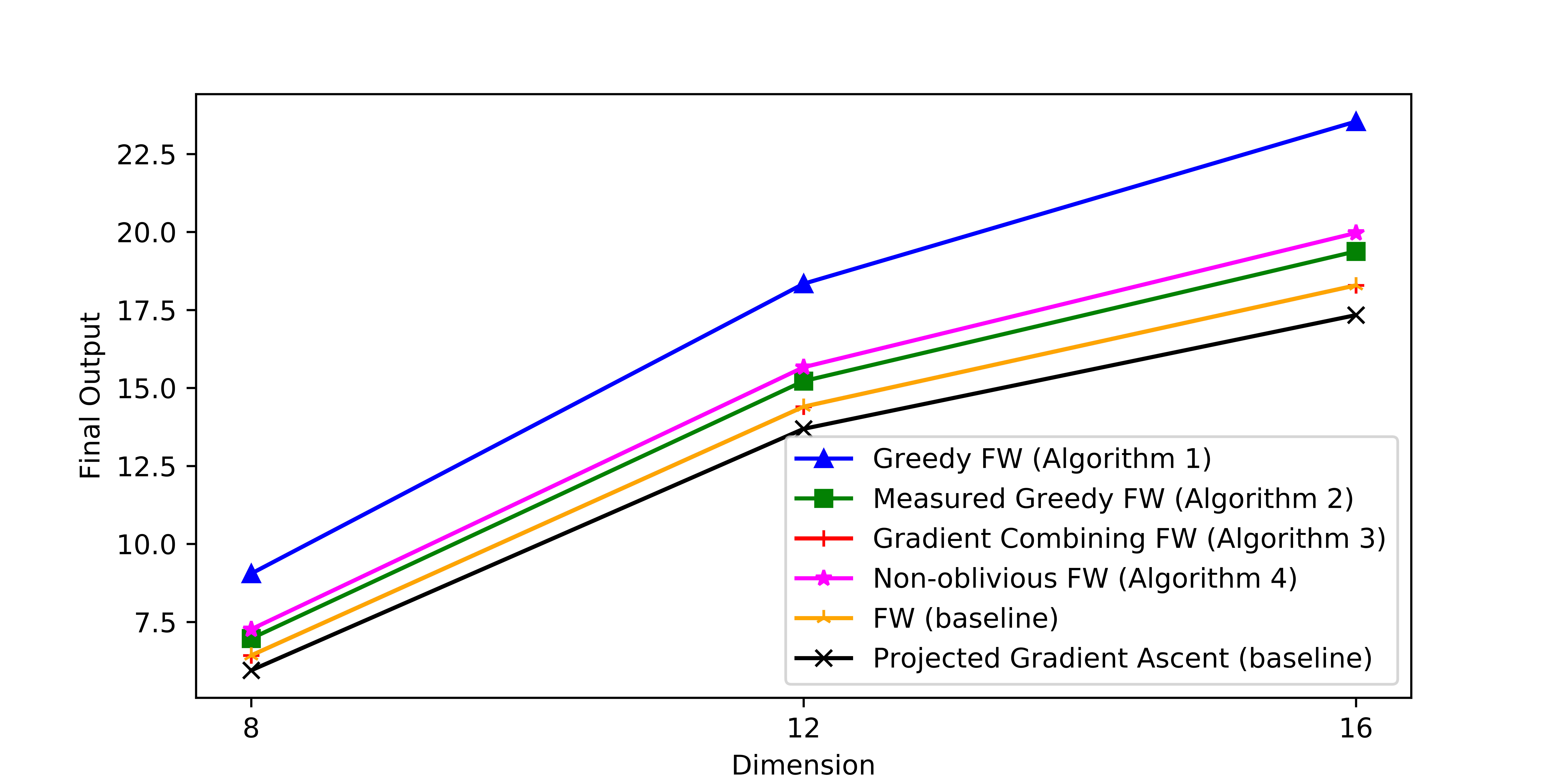
  • We then present experiments designed to use our algorithms to smoothly interpolate between contrasting objectives such as picking a diverse set of elements and picking a clustered set of elements. This smooth interpolation provides a way to control the amount of diversity in the final solution. We also demonstrate the use of our algorithms to maximize a large class of (non-convex/non-concave) quadratic programming problems.

Refer to caption
Figure 1: Left: (continuous) DR-submodular softmax extension. Middle: concave quadratic function. Right: sum of both.
Related Work.

The study of discrete submodular maximization has flourished in the last decade through far reaching applications in machine learning and and artificial intelligence including viral marketing (Kempe et al., 2003), dictionary learning (Krause and Cevher, 2010), sparse regression (Elenberg et al., 2016), neural network interoperability (Elenberg et al., 2017), crowd teaching (Singla et al., 2014), sequential decision making (Alieva et al., 2021), active learning (Wei et al., 2015), and data summarization (Mirzasoleiman et al., 2013). We refer the interested reader to a recent survey by Tohidi et al. (2020) and the references therein.

Recently, Bian et al. (2017b) proposed an extension of discrete submodular functions to the continuous domains that can be of use in machine learning applications. Notably, this class of (non-convex/non-concave) functions, so called continuous DR-submodular, contains the continuous multilinear extension of discrete submodular functions Călinescu et al. (2011) as a special case. Continuous DR-submodular functions can reliably model revenue maximization (Bian et al., 2017b), robust budget allocation (Staib and Jegelka, 2017), experimental design (Chen et al., 2018), MAP inference for DPPs (Gillenwater et al., 2012; Hassani et al., 2020b), energy allocation (Wilder, 2018a), classes of zero-sum games (Wilder, 2018b), online welfare maximization and online task assignment (Sadeghi et al., 2020), as well as many other settings of interest.

The research on maximizing continuous DR-submodular functions in the last few years has established strong theoretical results in different optimization settings including unconstrained (Niazadeh et al., 2018; Bian et al., 2019), stochastic Mokhtari et al. (2018a); Hassani et al. (2017), online (Chen et al., 2018; Zhang et al., 2019; Sadeghi and Fazel, 2019; Raut et al., 2021), and parallel models of computation (Chen et al., 2019a; Mokhtari et al., 2018b; Xie et al., 2019; Ene and Nguyen, 2019).

A different line of works study the maximization of discrete functions that can be represented as the sum of a non-negative monotone submodular function and a linear function. The ability to do so is useful in practice since the linear function can be viewed as a soft constraint, and it also has theoretical applications as is argued by the first work in this line (Sviridenko et al., 2017) (for example, the problem of maximization of a monotone submodular function with a bounded curvature can be reduced to the maximization of the sum of a monotone submodular function and a linear function). In terms of the approximation guarantee, the algorithms suggested by Sviridenko et al. (2017) were optimal. However, more recent works improve over the time complexities of these algorithms (Feldman, 2021; Harshaw et al., 2019; Ene et al., 2020), generalize them to weakly-submodular functions (Harshaw et al., 2019), and adapt them to other computational models such as the data stream and MapReduce models (Kazemi et al., 2020b; Ene et al., 2020).

2 Setting and Notation

Let us now formally define the setting we consider. Fix a subset \cX\cX\cX of Rnsuperscript𝑅𝑛R^{n} of the form i=1n\cXisuperscriptsubscriptproduct𝑖1𝑛subscript\cX𝑖\prod_{i=1}^{n}\cX_{i}, where \cXisubscript\cX𝑖\cX_{i} is a closed range in \bR\bR\bR. Intuitively, a function G:\cX\bR:𝐺\cX\bRG\colon\cX\to\bR is called (continuous) DR-submodular if it exhibits diminishing returns in the sense that given a vector \vx\cX\vx\cX\vx\in\cX, the increase in G(\vx)𝐺\vxG(\vx) obtained by increasing xisubscript𝑥𝑖x_{i} (for any i[n]𝑖delimited-[]𝑛i\in[n]) by ε>0𝜀0\varepsilon>0 is negatively correlated with the original values of the coordinates of \vx\vx\vx. This intuition is captured by the following definition. In this definition \veisubscript\ve𝑖\ve_{i} denotes the standard basis vector in the ithsuperscript𝑖thi^{\text{th}} direction.

Definition 2.1 (DR-submodular function).

A function G:\cX\bR:𝐺\cX\bRG\colon\cX\to\bR is DR-submodular if for every two vectors \va,\vb\cX\va\vb\cX\va,\vb\in\cX, positive value k𝑘k and coordinate i[n]𝑖delimited-[]𝑛i\in[n] we have

G(\va+k\vei)G(\va)G(\vb+k\vei)G(\vb)𝐺\va𝑘subscript\ve𝑖𝐺\va𝐺\vb𝑘subscript\ve𝑖𝐺\vbG(\va+k\ve_{i})-G(\va)\geq G(\vb+k\ve_{i})-G(\vb)

whenever \va\vb\va\vb\va\leq\vb and \va+k\vei,\vb+k\vei\cX\va𝑘subscript\ve𝑖\vb𝑘subscript\ve𝑖\cX\va+k\ve_{i},\vb+k\ve_{i}\in\cX.111Throughout the paper, inequalities between vectors should be understood as holding coordinate-wise.

It is well known that when G𝐺G is continuously differentiable, then it is DR-submodular if and only if G(\va)G(\vb)𝐺\va𝐺\vb\nabla G(\va)\geq\nabla G(\vb) for every two vectors \va,\vb\cX\va\vb\cX\va,\vb\in\cX that obey \va\vb\va\vb\va\leq\vb. And when G𝐺G is a twice differentiable function, it is DR-submodular if and only if its hessian is non-positive at every vector \vx\cX\vx\cX\vx\in\cX. Furthermore, for the sake of simplicity we assume in this work that \cX=[0,1]n\cXsuperscript01𝑛\cX=[0,1]^{n}. This assumption is without loss of generality because the natural mapping from \cX\cX\cX to [0,1]nsuperscript01𝑛[0,1]^{n} preserves all our results.

We are interested in the problem of finding the point in some convex body P[0,1]n𝑃superscript01𝑛P\subseteq[0,1]^{n} that maximizes a given function F:[0,1]n\bR:𝐹superscript01𝑛\bRF\colon[0,1]^{n}\to\bR that can be expressed as the sum of a DR-submodular function G:[0,1]n\bR:𝐺superscript01𝑛\bRG\colon[0,1]^{n}\to\bR and a concave function C:[0,1]n\bR:𝐶superscript01𝑛\bRC\colon[0,1]^{n}\to\bR. To get meaningful results for this problem, we need to make some assumptions. Here we describe three basic assumptions that we make throughout the paper. The quality of the results that we obtain improves if additional assumptions are made, as is described in Section 3.

Our first basic assumption is that G𝐺G is non-negative. This assumption is necessary since we obtain multiplicative approximation guarantees with respect to G𝐺G, and such guarantees do not make sense when G𝐺G is allowed to take negative values.222We note that almost all the literature on submodular maximization of both discrete and continuous functions assumes non-negativity for the same reason. Our second basic assumption is that P𝑃P is solvable, i.e., that one can efficiently optimize linear functions subject to it. Intuitively, this assumption makes sense because one should not expect to be able to optimize a complex function such as F𝐹F subject to P𝑃P if one cannot optimize linear functions subject to it (nevertheless, it is possible to adapt our algorithms to obtain some guarantee even when linear functions can only be approximately optimized subject to P𝑃P). Our final basic assumption is that both functions G𝐺G and C𝐶C are L𝐿L-smooth, which means that they are differentiable, and moreover, their gradients are L𝐿L-Lipschitz, i.e.,

f(\va)f(\vb)2L\va\vb2\va,\vb[0,1]n.formulae-sequencesubscriptnorm𝑓\va𝑓\vb2𝐿subscriptnorm\va\vb2for-all\va\vbsuperscript01𝑛\|\nabla f(\va)-\nabla f(\vb)\|_{2}\leq L\|\va-\vb\|_{2}\quad\forall\;\va,\vb\in[0,1]^{n}\enspace.

We conclude this section by introducing some additional notation that we need. We denote by \vo\vo\vo an arbitrary optimal solution for the problem described above, and define D=max\vxP\vx2𝐷subscript\vx𝑃subscriptnorm\vx2D=\max_{\vx\in P}\|\vx\|_{2}. Additionally, given two vectors \va,\vb\bRn\va\vbsuperscript\bR𝑛\va,\vb\in\bR^{n}, we denote by \va\vbdirect-product\va\vb\va\odot\vb their coordinate-wise multiplication, and by \va,\vb\va\vb\left\langle{\va,\vb}\right\rangle their standard Euclidean inner product.

3 Main Algorithms and Results

In this section we present our (first-order) algorithms for solving the problem described in Section 2. In general, these algorithms are all Frank-Wolfe type algorithms, but they differ in the exact linear function which is maximized in each iteration (step 1 of the while/for loop), and in the formula used to update the solution (step 2 of the while/for loop). As mentioned previously, we assume everywhere that G𝐺G is a non-negative L𝐿L-smooth DR-submodular function, C𝐶C is an L𝐿L-smooth concave function, and P𝑃P is a solvable convex body. Some of our algorithms require additional non-negativity and/or monotonicity assumptions on the functions G𝐺G and C𝐶C, and occasionally they also require a downward closed assumption on P𝑃P. A summary of which settings each algorithm is applicable to can be found in Table 1. Each algorithm listed in the table outputs a point xP𝑥𝑃x\in P which is guaranteed to obey F(x)αG(\vo)+βC(\vo)E𝐹𝑥𝛼𝐺\vo𝛽𝐶\vo𝐸F(x)\geq\alpha\cdot G(\vo)+\beta\cdot C(\vo)-E for the constants α𝛼\alpha and β𝛽\beta given in Table 1 and some error term E𝐸E.

Table 1: Summary of algorithms, settings, and guarantees (“non-neg.” is a shorthand for “non-negative”). All of the conditions stated in the table are in addition to the continuity and smoothness of G𝐺G and C𝐶C, and the convexity of P𝑃P. α𝛼\alpha and β𝛽\beta are the constants preceding G(\vo)𝐺\voG(\vo) and C(\vo)𝐶\voC(\vo) respectively in the lower bound on the output of the algorithm.

Algorithm (Section) G𝐺G C𝐶C P𝑃P α𝛼\alpha β𝛽\beta
Greedy monotone monotone general 11/e11𝑒1-1/e 11/e11𝑒1-1/e
Frank-Wolfe  & non-neg.  & non-neg.
Measured Greedy monotone non-neg. down-closed 11/e11𝑒1-1/e 1/e1𝑒1/e
Frank-Wolfe & non-neg.
Measured Greedy non-neg. monotone down-closed 1/e1𝑒1/e 11/e11𝑒1-1/e
Frank-Wolfe & non-neg.
Measured Greedy monotone monotone down-closed 11/e11𝑒1-1/e 11/e11𝑒1-1/e
Frank-Wolfe & non-neg. & non-neg.
Measured Greedy non-neg. non-neg. down-closed 1/e1𝑒1/e 1/e1𝑒1/e
Frank-Wolfe
Gradient Combining monotone General General 1/2ε12𝜀1/2-\varepsilon 1
Frank-Wolfe & non-neg.
Non-Oblivious monotone non-neg. General 11/eε11𝑒𝜀1-1/e-\varepsilon 1ε1𝜀1-\varepsilon
Frank-Wolfe & non-neg.

3.1 Greedy Frank-Wolfe Algorithm

In this section we assume that both G𝐺G and C𝐶C are monotone and non-negative functions (in addition to their other properties). Given this assumption, we analyze the guarantee of the greedy Frank-Wolfe variant appearing as Algorithm 1. This algorithm is related to the Continuous Greedy algorithm for discrete objective functions due to Călinescu et al. (2011), and it gets a quality control parameter ε(0,1)𝜀01\varepsilon\in(0,1). We assume in the algorithm that ε1superscript𝜀1\varepsilon^{-1} is an integer. This assumption is without loss of generality because, if ε𝜀\varepsilon violates the assumption, then it can be replaced with a value from the range [ε/2,ε]𝜀2𝜀[\varepsilon/2,\varepsilon] that obeys it.

  Let t0𝑡0t\leftarrow 0 and \vy(t)0¯superscript\vy𝑡¯0\vy^{(t)}\leftarrow{\bar{0}}
  while t<1𝑡1t<1 do
     \vs(t)argmax\vxPF(\vy(t)),\vxsuperscript\vs𝑡subscript\vx𝑃𝐹superscript\vy𝑡\vx\vs^{(t)}\leftarrow\arg\max_{\vx\in P}\left\langle{\nabla F(\vy^{(t)}),\vx}\right\rangle
     \vy(t+ε)\vy(t)+ε\vs(t)superscript\vy𝑡𝜀superscript\vy𝑡𝜀superscript\vs𝑡\vy^{(t+\varepsilon)}\leftarrow\vy^{(t)}+\varepsilon\cdot\vs^{(t)}
     tt+ε𝑡𝑡𝜀t\leftarrow t+\varepsilon
  end while
  return  \vy(1)superscript\vy1\vy^{(1)}
Algorithm 1 Greedy Frank-Wolfe (ε)𝜀(\varepsilon)

One can observe that the output \vy(1)superscript\vy1\vy^{(1)} of Algorithm 1 is within the convex body P𝑃P because it is a convex combination of the vectors \vs(0),\vs(ε),\vs(2ε),,\vs1εsuperscript\vs0superscript\vs𝜀superscript\vs2𝜀superscript\vs1𝜀\vs^{(0)},\vs^{(\varepsilon)},\vs^{(2\varepsilon)},\dotsc,\vs^{1-\varepsilon}, which are all vectors in P𝑃P. Let us now analyze the value of the output of Algorithm 1. The next lemma is the first step towards this goal. It provides a lower bounds on the increase in the value of \vy(t)superscript\vy𝑡\vy^{(t)} as a function of t𝑡t.

Lemma 3.1.

For every 0i<ε10𝑖superscript𝜀10\leq i<\varepsilon^{-1}, F(\vy(ε(i+1)))F(\vy(εi))ε[F(\vo)F(\vy(εi))]ε2LD2𝐹superscript\vy𝜀𝑖1𝐹superscript\vy𝜀𝑖𝜀delimited-[]𝐹\vo𝐹superscript\vy𝜀𝑖superscript𝜀2𝐿superscript𝐷2F(\vy^{(\varepsilon(i+1))})-F(\vy^{(\varepsilon i)})\geq\varepsilon\cdot[F(\vo)-F(\vy^{(\varepsilon i)})]-\varepsilon^{2}LD^{2}.

Proof.

Observe that

F(\vy(ε(i+1)))F(\displaystyle F(\vy^{(\varepsilon(i+1))})-F( \vy(εi))=F(\vy(εi)+ε\vs(εi))F(\vy(εi))=0εdF(\vy(εi)+z\vs(εi))dz|z=rdr\displaystyle\vy^{(\varepsilon i)})=F(\vy^{(\varepsilon i)}+\varepsilon\cdot\vs^{(\varepsilon i)})-F(\vy^{(\varepsilon i)})=\int_{0}^{\varepsilon}\left.\frac{dF(\vy^{(\varepsilon i)}+z\cdot\vs^{(\varepsilon i)})}{dz}\right|_{z=r}dr
=\displaystyle={} 0ε\vs(εi),F(\vy(εi)+r\vs(εi))𝑑r0ε{\vs(εi),F(\vy(εi))2rLD2}𝑑rsuperscriptsubscript0𝜀superscript\vs𝜀𝑖𝐹superscript\vy𝜀𝑖𝑟superscript\vs𝜀𝑖differential-d𝑟superscriptsubscript0𝜀superscript\vs𝜀𝑖𝐹superscript\vy𝜀𝑖2𝑟𝐿superscript𝐷2differential-d𝑟\displaystyle\int_{0}^{\varepsilon}\left\langle{\vs^{(\varepsilon i)},\nabla F(\vy^{(\varepsilon i)}+r\cdot\vs^{(\varepsilon i)})}\right\rangle dr\geq\int_{0}^{\varepsilon}\left\{\left\langle{\vs^{(\varepsilon i)},\nabla F(\vy^{(\varepsilon i)})}\right\rangle-2rLD^{2}\right\}dr
=\displaystyle={} ε\vs(εi),F(\vy(εi))ε2LD2ε\vo,F(\vy(εi))ε2LD2.𝜀superscript\vs𝜀𝑖𝐹superscript\vy𝜀𝑖superscript𝜀2𝐿superscript𝐷2𝜀\vo𝐹superscript\vy𝜀𝑖superscript𝜀2𝐿superscript𝐷2\displaystyle\left\langle{\varepsilon\vs^{(\varepsilon i)},\nabla F(\vy^{(\varepsilon i)})}\right\rangle-\varepsilon^{2}LD^{2}\geq\left\langle{\varepsilon\vo,\nabla F(\vy^{(\varepsilon i)})}\right\rangle-\varepsilon^{2}LD^{2}\enspace.

where the last inequality follows since \vs(εi)superscript\vs𝜀𝑖\vs^{(\varepsilon i)} is the maximizer found by Algorithm 1. Therefore, to prove the lemma it only remains to show that \vo,F(\vy(εi))F(\vo)F(\vy(εi))\vo𝐹superscript\vy𝜀𝑖𝐹\vo𝐹superscript\vy𝜀𝑖\left\langle{\vo,\nabla F(\vy^{(\varepsilon i)})}\right\rangle\geq F(\vo)-F(\vy^{(\varepsilon i)}).

Since C𝐶C is concave and monotone,

C(\vo)C(\vo\vy(εi))C(\vy(εi))+\vo\vy(εi)\vy(εi),C(\vy(εi))C(\vy(εi))+\vo,C(\vy(εi)).𝐶\vo𝐶\vosuperscript\vy𝜀𝑖𝐶superscript\vy𝜀𝑖\vosuperscript\vy𝜀𝑖superscript\vy𝜀𝑖𝐶superscript\vy𝜀𝑖𝐶superscript\vy𝜀𝑖\vo𝐶superscript\vy𝜀𝑖C(\vo)\leq C(\vo\vee\vy^{(\varepsilon i)})\leq C(\vy^{(\varepsilon i)})+\left\langle{\vo\vee\vy^{(\varepsilon i)}-\vy^{(\varepsilon i)},\nabla C(\vy^{(\varepsilon i)})}\right\rangle\leq C(\vy^{(\varepsilon i)})+\left\langle{\vo,\nabla C(\vy^{(\varepsilon i)})}\right\rangle\enspace.

Similarly, since G𝐺G is DR-submodular and monotone,

G(\vo)𝐺\voabsent\displaystyle G(\vo)\leq{} G(\vo\vy(εi))=G(\vy(εi))+01dG(y(εi)+z(\vo\vy(εi)\vy(εi)))dz|z=rdr𝐺\vosuperscript\vy𝜀𝑖𝐺superscript\vy𝜀𝑖evaluated-atsuperscriptsubscript01𝑑𝐺superscript𝑦𝜀𝑖𝑧\vosuperscript\vy𝜀𝑖superscript\vy𝜀𝑖𝑑𝑧𝑧𝑟𝑑𝑟\displaystyle G(\vo\vee\vy^{(\varepsilon i)})=G(\vy^{(\varepsilon i)})+\int_{0}^{1}\left.\frac{dG(y^{(\varepsilon i)}+z\cdot(\vo\vee\vy^{(\varepsilon i)}-\vy^{(\varepsilon i)}))}{dz}\right|_{z=r}dr
=\displaystyle={} G(\vy(εi))+01\vo\vy(εi)\vy(εi),G(\vy(εi)+r(\vo\vy(εi)\vy(εi)))𝑑r𝐺superscript\vy𝜀𝑖superscriptsubscript01\vosuperscript\vy𝜀𝑖superscript\vy𝜀𝑖𝐺superscript\vy𝜀𝑖𝑟\vosuperscript\vy𝜀𝑖superscript\vy𝜀𝑖differential-d𝑟\displaystyle G(\vy^{(\varepsilon i)})+\int_{0}^{1}\left\langle{\vo\vee\vy^{(\varepsilon i)}-\vy^{(\varepsilon i)},\nabla G(\vy^{(\varepsilon i)}+r\cdot(\vo\vee\vy^{(\varepsilon i)}-\vy^{(\varepsilon i)}))}\right\rangle dr
\displaystyle\leq{} G(\vy(εi))+\vo\vy(εi)\vy(εi),G(\vy(εi))G(\vy(εi))+\vo,G(\vy(εi)).𝐺superscript\vy𝜀𝑖\vosuperscript\vy𝜀𝑖superscript\vy𝜀𝑖𝐺superscript\vy𝜀𝑖𝐺superscript\vy𝜀𝑖\vo𝐺superscript\vy𝜀𝑖\displaystyle G(\vy^{(\varepsilon i)})+\left\langle{\vo\vee\vy^{(\varepsilon i)}-\vy^{(\varepsilon i)},\nabla G(\vy^{(\varepsilon i)})}\right\rangle\leq G(\vy^{(\varepsilon i)})+\left\langle{\vo,\nabla G(\vy^{(\varepsilon i)})}\right\rangle\enspace.

Adding the last two inequalities and rearranging gives the inequality \vo,F(\vy(εi))F(\vo)F(\vy(εi))\vo𝐹superscript\vy𝜀𝑖𝐹\vo𝐹superscript\vy𝜀𝑖\left\langle{\vo,\nabla F(\vy^{(\varepsilon i)})}\right\rangle\geq F(\vo)-F(\vy^{(\varepsilon i)}) that we wanted to prove. ∎

The corollary below follows by showing (via induction) that the inequality F(\vy(εi))[1(1ε)i]F(\vo)iε2LD2𝐹superscript\vy𝜀𝑖delimited-[]1superscript1𝜀𝑖𝐹\vo𝑖superscript𝜀2𝐿superscript𝐷2F(\vy^{(\varepsilon i)})\geq\big{[}1-\left(1-\varepsilon\right)^{i}\big{]}\cdot F(\vo)-i\cdot\varepsilon^{2}LD^{2} holds for every integer 0iε10𝑖superscript𝜀10\leq i\leq\varepsilon^{-1}, and then plugging in i=ε1𝑖superscript𝜀1i=\varepsilon^{-1}. The inductive step is proven using Lemma 3.1.

Corollary 3.2.

F(\vy(1))(1e1)F(\vo)O(εLD2)𝐹superscript\vy11superscript𝑒1𝐹\vo𝑂𝜀𝐿superscript𝐷2F(\vy^{(1)})\geq(1-e^{-1})\cdot F(\vo)-O(\varepsilon LD^{2}).

Proof.

We prove by induction that for every integer 0iε10𝑖superscript𝜀10\leq i\leq\varepsilon^{-1} we have

F(\vy(εi))[1(1ε)i]F(\vo)iε2LD2.𝐹superscript\vy𝜀𝑖delimited-[]1superscript1𝜀𝑖𝐹\vo𝑖superscript𝜀2𝐿superscript𝐷2F(\vy^{(\varepsilon i)})\geq\left[1-\left(1-\varepsilon\right)^{i}\right]\cdot F(\vo)-i\cdot\varepsilon^{2}LD^{2}\enspace. (1)

One can note that the corollary follows from this inequality by plugging i=ε1𝑖superscript𝜀1i=\varepsilon^{-1} since (1ε)ε1e1superscript1𝜀superscript𝜀1superscript𝑒1(1-\varepsilon)^{\varepsilon^{-1}}\leq e^{-1}.

For i=0𝑖0i=0, Inequality (1) follows from the non-negativity of F𝐹F (which follows from the non-negativity of G𝐺G and C𝐶C). Next, let us prove Inequality (1) for 1iε11𝑖superscript𝜀11\leq i\leq\varepsilon^{-1} assuming it holds for i1𝑖1i-1. By Lemma 3.1,

F(\vy(εi))𝐹superscript\vy𝜀𝑖absent\displaystyle F(\vy^{(\varepsilon i)})\geq{} F(\vy(ε(i1)))+ε[F(\vo)F(\vy(ε(i1)))]ε2LD2𝐹superscript\vy𝜀𝑖1𝜀delimited-[]𝐹\vo𝐹superscript\vy𝜀𝑖1superscript𝜀2𝐿superscript𝐷2\displaystyle F(\vy^{(\varepsilon(i-1))})+\varepsilon\cdot[F(\vo)-F(\vy^{(\varepsilon(i-1))})]-\varepsilon^{2}LD^{2}
=\displaystyle={} (1ε)F(\vy(ε(i1)))+εF(\vo)ε2LD21𝜀𝐹superscript\vy𝜀𝑖1𝜀𝐹\vosuperscript𝜀2𝐿superscript𝐷2\displaystyle(1-\varepsilon)\cdot F(\vy^{(\varepsilon(i-1))})+\varepsilon\cdot F(\vo)-\varepsilon^{2}LD^{2}
\displaystyle\geq{} (1ε){[1(1ε)i1]F(\vo)(i1)ε2LD2}+εF(\vo)ε2LD21𝜀delimited-[]1superscript1𝜀𝑖1𝐹\vo𝑖1superscript𝜀2𝐿superscript𝐷2𝜀𝐹\vosuperscript𝜀2𝐿superscript𝐷2\displaystyle(1-\varepsilon)\cdot\left\{\left[1-\left(1-\varepsilon\right)^{i-1}\right]\cdot F(\vo)-(i-1)\cdot\varepsilon^{2}LD^{2}\right\}+\varepsilon\cdot F(\vo)-\varepsilon^{2}LD^{2}
\displaystyle\geq{} [1(1ε)i]F(\vo)iε2LD2,delimited-[]1superscript1𝜀𝑖𝐹\vo𝑖superscript𝜀2𝐿superscript𝐷2\displaystyle\left[1-\left(1-\varepsilon\right)^{i}\right]\cdot F(\vo)-i\cdot\varepsilon^{2}LD^{2}\enspace,

where the second inequality holds due to the induction hypothesis. ∎

We are now ready to summarize the properties of Algorithm 1 in a theorem.

Theorem 3.3.

Let S𝑆S be the time it takes to find a point in P𝑃P maximizing a given liner function, then Algorithm 1 runs in O(ε1(n+S))𝑂superscript𝜀1𝑛𝑆O(\varepsilon^{-1}(n+S)) time, makes O(1/ε)𝑂1𝜀O(1/\varepsilon) calls to the gradient oracle, and outputs a vector \vy\vy\vy such that F(\vy)(11/e)F(\vo)O(εLD2)𝐹\vy11𝑒𝐹\vo𝑂𝜀𝐿superscript𝐷2F(\vy)\geq(1-1/e)\cdot F(\vo)-O(\varepsilon LD^{2}).

Proof.

The output guarantee of Theorem 3.3 follows directly from Corollary 3.2. The time and oracle complexity follows by observing that the algorithm’s while loop makes ε1superscript𝜀1\varepsilon^{-1} iterations, and each iteration requires O(n+S)𝑂𝑛𝑆O(n+S) time, in addition to making a single call to the gradient oracle. ∎

3.2 Measured Greedy Frank-Wolfe Algorithm

In this section we assume that P𝑃P is a down-closed body (in addition to being convex) and that G𝐺G and C𝐶C are both non-negative. Given these assumptions, we analyze the guarantee of the variant of Frank-Wolfe appearing as Algorithm 2, which is motivated by the Measured Continuous Greedy algorithm for discrete objective functions due to Feldman et al. (2011). We again have a quality control parameter ε(0,1)𝜀01\varepsilon\in(0,1), and assume (without loss of generality) that ε1superscript𝜀1\varepsilon^{-1} is an integer.

  Let t0𝑡0t\leftarrow 0 and \vy(t)0¯superscript\vy𝑡¯0\vy^{(t)}\leftarrow{\bar{0}}
  while t<1𝑡1t<1 do
     \vs(t)argmax\vxP(1¯\vy(t))F(\vy(t)),\vxsuperscript\vs𝑡subscript\vx𝑃direct-product¯1superscript\vy𝑡𝐹superscript\vy𝑡\vx\vs^{(t)}\leftarrow\arg\max_{\vx\in P}\langle({\bar{1}}-\vy^{(t)})\odot\nabla F(\vy^{(t)}),\vx\rangle
     \vy(t+ε)\vy(t)+ε(1¯\vy(t))\vs(t)superscript\vy𝑡𝜀superscript\vy𝑡direct-product𝜀¯1superscript\vy𝑡superscript\vs𝑡\vy^{(t+\varepsilon)}\leftarrow\vy^{(t)}+\varepsilon\cdot({\bar{1}}-\vy^{(t)})\odot\vs^{(t)}
     tt+ε𝑡𝑡𝜀t\leftarrow t+\varepsilon
  end while
  return  \vy(1)superscript\vy1\vy^{(1)}
Algorithm 2 Measured Greedy Frank-Wolfe (ε)𝜀(\varepsilon)

We begin the analysis of Algorithm 2 by bounding the range of the entries of the vectors \vy(t)superscript\vy𝑡\vy^{(t)}, which is proven by induction.

Lemma 3.4.

For every two integers 0iε10𝑖superscript𝜀10\leq i\leq\varepsilon^{-1} and 1jn1𝑗𝑛1\leq j\leq n, 0yj(εi)1(1ε)i10subscriptsuperscript𝑦𝜀𝑖𝑗1superscript1𝜀𝑖10\leq y^{(\varepsilon i)}_{j}\leq 1-(1-\varepsilon)^{i}\leq 1.

Proof.

We prove the lemma by induction on i𝑖i. For i=0𝑖0i=0 the lemma is trivial since yj(0)=0subscriptsuperscript𝑦0𝑗0y^{(0)}_{j}=0 by the initialization of \vy(0)superscript\vy0\vy^{(0)}. Assume now that the lemma holds for i1𝑖1i-1, and let us prove it for 1iε11𝑖superscript𝜀11\leq i\leq\varepsilon^{-1}. Observe that

yj(εi)=yj(ε(i1))+ε(1yj(ε(i1)))sj(εi)yj(ε(i1))0,subscriptsuperscript𝑦𝜀𝑖𝑗subscriptsuperscript𝑦𝜀𝑖1𝑗𝜀1subscriptsuperscript𝑦𝜀𝑖1𝑗subscriptsuperscript𝑠𝜀𝑖𝑗subscriptsuperscript𝑦𝜀𝑖1𝑗0y^{(\varepsilon i)}_{j}=y^{(\varepsilon(i-1))}_{j}+\varepsilon\cdot(1-y^{(\varepsilon(i-1))}_{j})\cdot s^{(\varepsilon i)}_{j}\geq y^{(\varepsilon(i-1))}_{j}\geq 0\enspace,

where the first inequality holds since yj(ε(i1))1subscriptsuperscript𝑦𝜀𝑖1𝑗1y^{(\varepsilon(i-1))}_{j}\leq 1 by the induction hypothesis and sj(εi)0subscriptsuperscript𝑠𝜀𝑖𝑗0s^{(\varepsilon i)}_{j}\geq 0 since \vs(εi)Psuperscript\vs𝜀𝑖𝑃\vs^{(\varepsilon i)}\in P. Similarly,

yj(εi)=subscriptsuperscript𝑦𝜀𝑖𝑗absent\displaystyle y^{(\varepsilon i)}_{j}={} yj(ε(i1))+ε(1yj(ε(i1)))sj(εi)yj(ε(i1))+ε(1yj(ε(i1)))subscriptsuperscript𝑦𝜀𝑖1𝑗𝜀1subscriptsuperscript𝑦𝜀𝑖1𝑗subscriptsuperscript𝑠𝜀𝑖𝑗subscriptsuperscript𝑦𝜀𝑖1𝑗𝜀1subscriptsuperscript𝑦𝜀𝑖1𝑗\displaystyle y^{(\varepsilon(i-1))}_{j}+\varepsilon\cdot(1-y^{(\varepsilon(i-1))}_{j})\cdot s^{(\varepsilon i)}_{j}\leq y^{(\varepsilon(i-1))}_{j}+\varepsilon\cdot(1-y^{(\varepsilon(i-1))}_{j})
=\displaystyle={} ε+(1ε)yj(ε(i1))ε+(1ε)[1(1ε)i1]=1(1ε)i,𝜀1𝜀subscriptsuperscript𝑦𝜀𝑖1𝑗𝜀1𝜀delimited-[]1superscript1𝜀𝑖11superscript1𝜀𝑖\displaystyle\varepsilon+(1-\varepsilon)\cdot y^{(\varepsilon(i-1))}_{j}\leq\varepsilon+(1-\varepsilon)\cdot[1-(1-\varepsilon)^{i-1}]=1-(1-\varepsilon)^{i}\enspace,

where the first inequality holds because sj(εi)1subscriptsuperscript𝑠𝜀𝑖𝑗1s^{(\varepsilon i)}_{j}\leq 1 since \vs(εi)Psuperscript\vs𝜀𝑖𝑃\vs^{(\varepsilon i)}\in P, and the second inequality holds by the induction hypothesis. ∎

Using the last lemma, we can see why the output of Algorithm 2 must be in P𝑃P. Recall that the output of Algorithm 2 is \vy(1)=i=1ε1ε(1¯\vyε(i1))\vs(εi)εi=1ε1\vs(εi),superscript\vy1superscriptsubscript𝑖1superscript𝜀1direct-product𝜀¯1superscript\vy𝜀𝑖1superscript\vs𝜀𝑖𝜀superscriptsubscript𝑖1superscript𝜀1superscript\vs𝜀𝑖\vy^{(1)}=\sum_{i=1}^{\varepsilon^{-1}}\varepsilon\cdot({\bar{1}}-\vy^{\varepsilon(i-1)})\odot\vs^{(\varepsilon i)}\leq\varepsilon\cdot\sum_{i=1}^{\varepsilon^{-1}}\vs^{(\varepsilon i)}, where the inequality follows due to Lemma 3.4 and the fact that \vs(εi)superscript\vs𝜀𝑖\vs^{(\varepsilon i)} (as a vector in P𝑃P) is non-negative. Since εi=1ε1\vs(εi)𝜀superscriptsubscript𝑖1superscript𝜀1superscript\vs𝜀𝑖\varepsilon\cdot\sum_{i=1}^{\varepsilon^{-1}}\vs^{(\varepsilon i)} is a convex combination of points in P𝑃P, it also belongs to P𝑃P. Since the vector \vy(1)superscript\vy1\vy^{(1)} is coordinate-wise dominated by this combination, the down-closeness of P𝑃P implies \vy(1)Psuperscript\vy1𝑃\vy^{(1)}\in P.

Our next objective is to prove an approximation guarantee for Algorithm 2. Towards this goal, let us define, for every function H𝐻H, the expression M(H,i)𝑀𝐻𝑖M(H,i) to be 111 when H𝐻H is monotone and (1ε)isuperscript1𝜀𝑖(1-\varepsilon)^{i} when H𝐻H is non-monotone. Using this definition, we can state the following lemma and corollary, which are counterparts of Lemma 3.1 and Corollary 3.2 from Section 3.1.

Lemma 3.5.

For every integer 0i<ε10𝑖superscript𝜀10\leq i<\varepsilon^{-1}, F(\vy(ε(i+1)))F(\vy(εi))ε{[M(G,i)G(\vo)G(\vy(εi))]+[M(C,i)C(\vo)C(\vy(εi))]}ε2LD2𝐹superscript\vy𝜀𝑖1𝐹superscript\vy𝜀𝑖𝜀delimited-[]𝑀𝐺𝑖𝐺\vo𝐺superscript\vy𝜀𝑖delimited-[]𝑀𝐶𝑖𝐶\vo𝐶superscript\vy𝜀𝑖superscript𝜀2𝐿superscript𝐷2F(\vy^{(\varepsilon(i+1))})-F(\vy^{(\varepsilon i)})\geq\varepsilon\cdot\{[M(G,i)\cdot G(\vo)-G(\vy^{(\varepsilon i)})]+[M(C,i)\cdot C(\vo)-C(\vy^{(\varepsilon i)})]\}-\varepsilon^{2}LD^{2}.

Proof.

Observe that

F(\vy(ε(i+1)))F(\vy(εi))=𝐹superscript\vy𝜀𝑖1𝐹superscript\vy𝜀𝑖absent\displaystyle F(\vy^{(\varepsilon(i+1))})-F(\vy^{(\varepsilon i)})={} F(\vy(εi)+ε(1¯\vy(εi))\vs(εi))F(\vy(εi))𝐹superscript\vy𝜀𝑖direct-product𝜀¯1superscript\vy𝜀𝑖superscript\vs𝜀𝑖𝐹superscript\vy𝜀𝑖\displaystyle F(\vy^{(\varepsilon i)}+\varepsilon\cdot({\bar{1}}-\vy^{(\varepsilon i)})\odot\vs^{(\varepsilon i)})-F(\vy^{(\varepsilon i)})
=\displaystyle={} 0εdF(\vy(εi)+z(1¯\vy(εi))\vs(εi))dz|z=rdrevaluated-atsuperscriptsubscript0𝜀𝑑𝐹superscript\vy𝜀𝑖direct-product𝑧¯1superscript\vy𝜀𝑖superscript\vs𝜀𝑖𝑑𝑧𝑧𝑟𝑑𝑟\displaystyle\int_{0}^{\varepsilon}\left.\frac{dF(\vy^{(\varepsilon i)}+z\cdot({\bar{1}}-\vy^{(\varepsilon i)})\odot\vs^{(\varepsilon i)})}{dz}\right|_{z=r}dr
=\displaystyle={} 0ε(1¯\vy(εi))\vs(εi),F(\vy(εi)+r(1¯\vy(t))\vs(εi))𝑑rsuperscriptsubscript0𝜀direct-product¯1superscript\vy𝜀𝑖superscript\vs𝜀𝑖𝐹superscript\vy𝜀𝑖direct-product𝑟¯1superscript\vy𝑡superscript\vs𝜀𝑖differential-d𝑟\displaystyle\int_{0}^{\varepsilon}\left\langle{({\bar{1}}-\vy^{(\varepsilon i)})\odot\vs^{(\varepsilon i)},\nabla F(\vy^{(\varepsilon i)}+r\cdot({\bar{1}}-\vy^{(t)})\odot\vs^{(\varepsilon i)})}\right\rangle dr
\displaystyle\geq{} 0ε{((1¯\vy(εi))\vs(εi),F(\vy(εi))2rLD2}dr\displaystyle\int_{0}^{\varepsilon}\left\{\left\langle{(({\bar{1}}-\vy^{(\varepsilon i)})\odot\vs^{(\varepsilon i)},\nabla F(\vy^{(\varepsilon i)})}\right\rangle-2rLD^{2}\right\}dr
=\displaystyle={} ε(1¯\vy(εi))\vs(εi),F(\vy(εi))ε2LD2.direct-product𝜀¯1superscript\vy𝜀𝑖superscript\vs𝜀𝑖𝐹superscript\vy𝜀𝑖superscript𝜀2𝐿superscript𝐷2\displaystyle\left\langle{\varepsilon({\bar{1}}-\vy^{(\varepsilon i)})\odot\vs^{(\varepsilon i)},\nabla F(\vy^{(\varepsilon i)})}\right\rangle-\varepsilon^{2}LD^{2}\enspace.

Furthermore, we also have

(1¯\vy(εi))\vs(εi),F(\vy(εi))=direct-product¯1superscript\vy𝜀𝑖superscript\vs𝜀𝑖𝐹superscript\vy𝜀𝑖absent\displaystyle\left\langle{({\bar{1}}-\vy^{(\varepsilon i)})\odot\vs^{(\varepsilon i)},\nabla F(\vy^{(\varepsilon i)})}\right\rangle={} \vs(εi),(1¯\vy(εi))F(\vy(εi))superscript\vs𝜀𝑖direct-product¯1superscript\vy𝜀𝑖𝐹superscript\vy𝜀𝑖\displaystyle\left\langle{\vs^{(\varepsilon i)},({\bar{1}}-\vy^{(\varepsilon i)})\odot\nabla F(\vy^{(\varepsilon i)})}\right\rangle
\displaystyle\geq{} \vo,(1¯\vy(εi))F(\vy(εi)),\vodirect-product¯1superscript\vy𝜀𝑖𝐹superscript\vy𝜀𝑖\displaystyle\left\langle{\vo,({\bar{1}}-\vy^{(\varepsilon i)})\odot\nabla F(\vy^{(\varepsilon i)})}\right\rangle\enspace,

where the inequality holds since s(εi)superscript𝑠𝜀𝑖s^{(\varepsilon i)} is the maximizer found by Algorithm 2. Combining the last two inequalities, we get

F(\vy(ε(i+1)))F(\vy(εi))ε\vo,(1¯\vy(εi))F(\vy(εi))ε2LD2.𝐹superscript\vy𝜀𝑖1𝐹superscript\vy𝜀𝑖𝜀\vodirect-product¯1superscript\vy𝜀𝑖𝐹superscript\vy𝜀𝑖superscript𝜀2𝐿superscript𝐷2F(\vy^{(\varepsilon(i+1))})-F(\vy^{(\varepsilon i)})\geq\left\langle{\varepsilon\vo,({\bar{1}}-\vy^{(\varepsilon i)})\odot\nabla F(\vy^{(\varepsilon i)})}\right\rangle-\varepsilon^{2}LD^{2}\enspace. (2)

Let us now find a lower bound on the expression \vo,(1¯\vy(εi))F(\vy(εi))\vodirect-product¯1superscript\vy𝜀𝑖𝐹superscript\vy𝜀𝑖\left\langle{\vo,({\bar{1}}-\vy^{(\varepsilon i)})\odot\nabla F(\vy^{(\varepsilon i)})}\right\rangle in the above inequality. Since C𝐶C is concave,

C(\vo(1¯\vy(εi))+\vy(εi))C(\vy(εi))𝐶direct-product\vo¯1superscript\vy𝜀𝑖superscript\vy𝜀𝑖𝐶superscript\vy𝜀𝑖absent\displaystyle C(\vo\odot({\bar{1}}-\vy^{(\varepsilon i)})+\vy^{(\varepsilon i)})-C(\vy^{(\varepsilon i)})\leq{} \vo(1¯\vy(εi)),C(\vy(εi))direct-product\vo¯1superscript\vy𝜀𝑖𝐶superscript\vy𝜀𝑖\displaystyle\left\langle{\vo\odot({\bar{1}}-\vy^{(\varepsilon i)}),\nabla C(\vy^{(\varepsilon i)})}\right\rangle
=\displaystyle={} \vo,(1¯\vy(εi))C(\vy(εi)).\vodirect-product¯1superscript\vy𝜀𝑖𝐶superscript\vy𝜀𝑖\displaystyle\left\langle{\vo,({\bar{1}}-\vy^{(\varepsilon i)})\odot\nabla C(\vy^{(\varepsilon i)})}\right\rangle\enspace.

Similarly, since G𝐺G is DR-submodular,

G(\vo(1¯\vy(εi))+\vy(εi))𝐺direct-product\vo¯1superscript\vy𝜀𝑖superscript\vy𝜀𝑖\displaystyle G(\vo\odot({\bar{1}}-\vy^{(\varepsilon i)})+\vy^{(\varepsilon i)}) G(\vy(εi))=01dG(\vy(εi)+z\vo(1¯\vy(εi))dz|z=rdr\displaystyle{}-G(\vy^{(\varepsilon i)})=\int_{0}^{1}\left.\frac{dG(\vy^{(\varepsilon i)}+z\cdot\vo\odot({\bar{1}}-\vy^{(\varepsilon i)})}{dz}\right|_{z=r}dr
=\displaystyle={} 01\vo(1¯\vy(εi)),G(\vy(εi)+r\vo(1¯\vy(εi)))𝑑rsuperscriptsubscript01direct-product\vo¯1superscript\vy𝜀𝑖𝐺superscript\vy𝜀𝑖direct-product𝑟\vo¯1superscript\vy𝜀𝑖differential-d𝑟\displaystyle\int_{0}^{1}\left\langle{\vo\odot({\bar{1}}-\vy^{(\varepsilon i)}),\nabla G(\vy^{(\varepsilon i)}+r\cdot\vo\odot({\bar{1}}-\vy^{(\varepsilon i)}))}\right\rangle dr
\displaystyle\leq{} \vo(1¯\vy(εi)),G(\vy(εi))\vo,(1¯\vy(t))G(\vy(εi)).direct-product\vo¯1superscript\vy𝜀𝑖𝐺superscript\vy𝜀𝑖\vodirect-product¯1superscript\vy𝑡𝐺superscript\vy𝜀𝑖\displaystyle\left\langle{\vo\odot({\bar{1}}-\vy^{(\varepsilon i)}),\nabla G(\vy^{(\varepsilon i)})}\right\rangle\leq\left\langle{\vo,({\bar{1}}-\vy^{(t)})\odot\nabla G(\vy^{(\varepsilon i)})}\right\rangle\enspace.

Adding the last two inequalities provides the promised lower bound on \vo,(1¯\vy(t))F(\vy(εi))\vodirect-product¯1superscript\vy𝑡𝐹superscript\vy𝜀𝑖\left\langle{\vo,({\bar{1}}-\vy^{(t)})\odot\nabla F(\vy^{(\varepsilon i)})}\right\rangle. Plugging this lower bound into Inequality (2) yields

F(\vy(ε(i+1)))F(\vy(εi))ε{\displaystyle F(\vy^{(\varepsilon(i+1))})-F(\vy^{(\varepsilon i)})\geq\varepsilon\cdot\{ [G(\vo(1¯\vy(εi))+\vy(εi))G(\vy(εi))]delimited-[]𝐺direct-product\vo¯1superscript\vy𝜀𝑖superscript\vy𝜀𝑖𝐺superscript\vy𝜀𝑖\displaystyle[G(\vo\odot({\bar{1}}-\vy^{(\varepsilon i)})+\vy^{(\varepsilon i)})-G(\vy^{(\varepsilon i)})]
+[C(\vo(1¯\vy(εi))+\vy(εi))C(\vy(εi))]}ε2LD2.\displaystyle+[C(\vo\odot({\bar{1}}-\vy^{(\varepsilon i)})+\vy^{(\varepsilon i)})-C(\vy^{(\varepsilon i)})]\}-\varepsilon^{2}LD^{2}\enspace.

Given the last inequality, to prove the lemma it remains to show that G(\vo(1¯\vy(εi))+\vy(εi))M(G,i)G(\vo)𝐺direct-product\vo¯1superscript\vy𝜀𝑖superscript\vy𝜀𝑖𝑀𝐺𝑖𝐺\voG(\vo\odot({\bar{1}}-\vy^{(\varepsilon i)})+\vy^{(\varepsilon i)})\geq M(G,i)\cdot G(\vo) and C(\vo(1¯\vy(εi))+\vy(εi))M(C,i)C(\vo)𝐶direct-product\vo¯1superscript\vy𝜀𝑖superscript\vy𝜀𝑖𝑀𝐶𝑖𝐶\voC(\vo\odot({\bar{1}}-\vy^{(\varepsilon i)})+\vy^{(\varepsilon i)})\geq M(C,i)\cdot C(\vo). Since \vo(1¯\vy(εi))+\vy(εi)\vodirect-product\vo¯1superscript\vy𝜀𝑖superscript\vy𝜀𝑖\vo\vo\odot({\bar{1}}-\vy^{(\varepsilon i)})+\vy^{(\varepsilon i)}\geq\vo, these inequalities follow immediately when G𝐺G and C𝐶C are monotone, respectively. Therefore, we concentrate on proving these inequalities when G𝐺G and C𝐶C are non-monotone. Since C𝐶C is concave,

C(\vo(1¯\displaystyle C(\vo\odot({\bar{1}}-{} \vy(εi))+\vy(εi))\displaystyle\vy^{(\varepsilon i)})+\vy^{(\varepsilon i)})
=\displaystyle={} C(M(C,i)\vo+(1M(C,i))((1M(C,i))1¯\vy(εi))\vo+\vy(εi)1M(C,i))𝐶𝑀𝐶𝑖\vo1𝑀𝐶𝑖direct-product1𝑀𝐶𝑖¯1superscript\vy𝜀𝑖\vosuperscript\vy𝜀𝑖1𝑀𝐶𝑖\displaystyle C\left(\mspace{-6.0mu}M(C,i)\cdot\vo+(1-M(C,i))\cdot\frac{((1-M(C,i))\cdot{\bar{1}}-\vy^{(\varepsilon i)})\odot\vo+\vy^{(\varepsilon i)}}{1-M(C,i)}\right)
\displaystyle\geq{} M(C,i)C(\vo)+(1M(C,i))C(((1M(C,i))1¯\vy(εi))\vo+\vy(εi)1M(C,i))𝑀𝐶𝑖𝐶\vo1𝑀𝐶𝑖𝐶direct-product1𝑀𝐶𝑖¯1superscript\vy𝜀𝑖\vosuperscript\vy𝜀𝑖1𝑀𝐶𝑖\displaystyle M(C,i)\cdot C(\vo)+(1-M(C,i))\cdot C\left(\frac{((1-M(C,i))\cdot{\bar{1}}-\vy^{(\varepsilon i)})\odot\vo+\vy^{(\varepsilon i)}}{1-M(C,i)}\right)
\displaystyle\geq{} M(C,i)C(\vo),𝑀𝐶𝑖𝐶\vo\displaystyle M(C,i)\cdot C(\vo)\enspace,

where the second inequality follows from the non-negativity of C𝐶C. We also note that

((1M(C,i))1¯\vy(εi))\vo+\vy(εi)1M(C,i)[0,1]ndirect-product1𝑀𝐶𝑖¯1superscript\vy𝜀𝑖\vosuperscript\vy𝜀𝑖1𝑀𝐶𝑖superscript01𝑛\frac{((1-M(C,i))\cdot{\bar{1}}-\vy^{(\varepsilon i)})\odot\vo+\vy^{(\varepsilon i)}}{1-M(C,i)}\in[0,1]^{n}

since 0\vy(εi)(1M(C,i))1¯0superscript\vy𝜀𝑖1𝑀𝐶𝑖¯10\leq\vy^{(\varepsilon i)}\leq(1-M(C,i))\cdot{\bar{1}} by Lemma 3.4. Similarly, since G𝐺G is DR-submodular,

G(\vo(1¯\displaystyle G(\vo\odot({\bar{1}} \vy(εi))+\vy(εi))=G(\vo+(1¯\vo)\vy(εi))\displaystyle{}-\vy^{(\varepsilon i)})+\vy^{(\varepsilon i)})=G(\vo+({\bar{1}}-\vo)\odot\vy^{(\varepsilon i)})
=\displaystyle={} G(\vo)+01dG(\vo+z(1¯\vo)\vy(εi))dz|z=rdr𝐺\voevaluated-atsuperscriptsubscript01𝑑𝐺\vodirect-product𝑧¯1\vosuperscript\vy𝜀𝑖𝑑𝑧𝑧𝑟𝑑𝑟\displaystyle G(\vo)+\int_{0}^{1}\left.\frac{dG(\vo+z\cdot({\bar{1}}-\vo)\odot\vy^{(\varepsilon i)})}{dz}\right|_{z=r}dr
\displaystyle\geq{} G(\vo)+(1M(G,i))0(1M(G,i))1dG(\vo+z(1¯\vo)\vy(εi))dz|z=rdr𝐺\voevaluated-at1𝑀𝐺𝑖superscriptsubscript0superscript1𝑀𝐺𝑖1𝑑𝐺\vodirect-product𝑧¯1\vosuperscript\vy𝜀𝑖𝑑𝑧𝑧𝑟𝑑𝑟\displaystyle G(\vo)+(1-M(G,i))\cdot\int_{0}^{(1-M(G,i))^{-1}}\left.\frac{dG(\vo+z\cdot({\bar{1}}-\vo)\odot\vy^{(\varepsilon i)})}{dz}\right|_{z=r}dr
=\displaystyle={} M(G,i)G(\vo)+(1M(G,i))G(\vo+11M(G,i)(1¯\vo)\vy(εi))𝑀𝐺𝑖𝐺\vo1𝑀𝐺𝑖𝐺\vodirect-product11𝑀𝐺𝑖¯1\vosuperscript\vy𝜀𝑖\displaystyle M(G,i)\cdot G(\vo)+(1-M(G,i))\cdot G\left(\vo+\frac{1}{1-M(G,i)}\cdot({\bar{1}}-\vo)\odot\vy^{(\varepsilon i)}\right)
\displaystyle\geq{} M(G,i)G(\vo),𝑀𝐺𝑖𝐺\vo\displaystyle M(G,i)\cdot G(\vo)\enspace,

where the second inequality follows from the non-negativity of G𝐺G, and the first inequality holds since

\vo+11M(G,i)(1¯\vo)\vy(εi)[0,1]n\vodirect-product11𝑀𝐺𝑖¯1\vosuperscript\vy𝜀𝑖superscript01𝑛\vo+\frac{1}{1-M(G,i)}\cdot({\bar{1}}-\vo)\odot\vy^{(\varepsilon i)}\in[0,1]^{n}

because 0\vy(εi)(1M(C,i))1¯0superscript\vy𝜀𝑖1𝑀𝐶𝑖¯10\leq\vy^{(\varepsilon i)}\leq(1-M(C,i))\cdot{\bar{1}} by Lemma 3.4. ∎

Corollary 3.6.
F(\vy(1)){1e1if G is monotonee1otherwise}G(\vo)+{1e1if C is monotonee1otherwise}C(\vo)O(εLD2).𝐹superscript\vy11superscript𝑒1if G is monotonesuperscript𝑒1otherwise𝐺\vo1superscript𝑒1if C is monotonesuperscript𝑒1otherwise𝐶\vo𝑂𝜀𝐿superscript𝐷2F(\vy^{(1)})\mspace{-3.0mu}\geq\mspace{-3.0mu}\left\{\begin{array}[]{ll}\mspace{-8.0mu}1-e^{-1}\mspace{-7.0mu}&\text{if $G$ is monotone}\mspace{-8.0mu}\\ \mspace{-8.0mu}e^{-1}&\text{otherwise}\end{array}\right\}\cdot G(\vo)+\left\{\begin{array}[]{ll}\mspace{-8.0mu}1-e^{-1}\mspace{-7.0mu}&\text{if $C$ is monotone}\mspace{-8.0mu}\\ \mspace{-8.0mu}e^{-1}&\text{otherwise}\end{array}\right\}\cdot C(\vo)-O(\varepsilon LD^{2})\mspace{-2.0mu}\enspace.
Proof.

For every function H𝐻H, let S(H,i)𝑆𝐻𝑖S(H,i) be 1(1ε)i1superscript1𝜀𝑖1-(1-\varepsilon)^{i} if H𝐻H is monotone, and (εi)(1ε)i1𝜀𝑖superscript1𝜀𝑖1(\varepsilon i)\cdot(1-\varepsilon)^{i-1} if H𝐻H is non-monotone. We prove by induction that for every integer 0iε10𝑖superscript𝜀10\leq i\leq\varepsilon^{-1} we have

F(\vy(εi))S(G,i)G(\vo)+S(C,i)C(\vo)iε2LD2.𝐹superscript\vy𝜀𝑖𝑆𝐺𝑖𝐺\vo𝑆𝐶𝑖𝐶\vo𝑖superscript𝜀2𝐿superscript𝐷2F(\vy^{(\varepsilon i)})\geq S(G,i)\cdot G(\vo)+S(C,i)\cdot C(\vo)-i\cdot\varepsilon^{2}LD^{2}\enspace. (3)

One can note that the corollary follows from this inequality by plugging i=ε1𝑖superscript𝜀1i=\varepsilon^{-1} since S(H,ε1)=1(1ε)ε11e1𝑆𝐻superscript𝜀11superscript1𝜀superscript𝜀11superscript𝑒1S(H,\varepsilon^{-1})=1-(1-\varepsilon)^{\varepsilon^{-1}}\geq 1-e^{-1} when H𝐻H is monotone and S(H,ε1)=(1ε)ε11e1𝑆𝐻superscript𝜀1superscript1𝜀superscript𝜀11superscript𝑒1S(H,\varepsilon^{-1})=(1-\varepsilon)^{\varepsilon^{-1}-1}\geq e^{-1} when H𝐻H is non-monotone.

For i=0𝑖0i=0, Inequality (3) follows from the non-negativity of F𝐹F since S(H,0)=0𝑆𝐻00S(H,0)=0 both when H𝐻H is monotone and non-monotone. Next, let us prove Inequality (3) for 1iε11𝑖superscript𝜀11\leq i\leq\varepsilon^{-1} assuming it holds for i1𝑖1i-1. We note that (1ε)S(H,i1)+εM(H,i1)=S(H,i)1𝜀𝑆𝐻𝑖1𝜀𝑀𝐻𝑖1𝑆𝐻𝑖(1-\varepsilon)\cdot S(H,i-1)+\varepsilon\cdot M(H,i-1)=S(H,i). For a monotone H𝐻H this is true since

(1ε)S(H,i1)+εM(H,i1)=(1ε)[1(1ε)i1]+ε=1(1ε)i=S(H,i),1𝜀𝑆𝐻𝑖1𝜀𝑀𝐻𝑖11𝜀delimited-[]1superscript1𝜀𝑖1𝜀1superscript1𝜀𝑖𝑆𝐻𝑖(1-\varepsilon)\cdot S(H,i-1)+\varepsilon\cdot M(H,i-1)=(1-\varepsilon)\cdot[1-(1-\varepsilon)^{i-1}]+\varepsilon=1-(1-\varepsilon)^{i}=S(H,i)\enspace,

and for a non-monotone H𝐻H this is true since

(1ε)S(H,i1)+εM(H,i1)=1𝜀𝑆𝐻𝑖1𝜀𝑀𝐻𝑖1absent\displaystyle(1-\varepsilon)\cdot S(H,i-1)+\varepsilon\cdot M(H,i-1)={} (1ε)(ε(i1))(1ε)i2+ε(1ε)i11𝜀𝜀𝑖1superscript1𝜀𝑖2𝜀superscript1𝜀𝑖1\displaystyle(1-\varepsilon)\cdot(\varepsilon(i-1))\cdot(1-\varepsilon)^{i-2}+\varepsilon\cdot(1-\varepsilon)^{i-1}
=\displaystyle={} (εi)(1ε)i1=S(H,i).𝜀𝑖superscript1𝜀𝑖1𝑆𝐻𝑖\displaystyle(\varepsilon i)\cdot(1-\varepsilon)^{i-1}=S(H,i)\enspace.

Using Lemma 3.5, we now get

F(\vy(εi))𝐹superscript\vy𝜀𝑖absent\displaystyle F(\vy^{(\varepsilon i)})\geq{} F(\vy(ε(i1)))+ε{[M(G,i1)G(\vo)G(\vy(ε(i1)))]\displaystyle F(\vy^{(\varepsilon(i-1))})+\varepsilon\cdot\{[M(G,i-1)\cdot G(\vo)-G(\vy^{(\varepsilon(i-1))})]
+[M(C,i1)C(\vo)C(\vy(ε(i1)))]}ε2LD2\displaystyle\mspace{200.0mu}+[M(C,i-1)\cdot C(\vo)-C(\vy^{(\varepsilon(i-1))})]\}-\varepsilon^{2}LD^{2}
=\displaystyle={} (1ε)F(\vy(ε(i1)))+ε{M(G,i1)G(\vo)+M(C,i1)C(\vo)}ε2LD21𝜀𝐹superscript\vy𝜀𝑖1𝜀𝑀𝐺𝑖1𝐺\vo𝑀𝐶𝑖1𝐶\vosuperscript𝜀2𝐿superscript𝐷2\displaystyle(1-\varepsilon)\cdot F(\vy^{(\varepsilon(i-1))})+\varepsilon\cdot\{M(G,i-1)\cdot G(\vo)+M(C,i-1)\cdot C(\vo)\}-\varepsilon^{2}LD^{2}
\displaystyle\geq{} [(1ε)S(G,i1)G(\vo)+εM(G,i1)G(\vo)]delimited-[]1𝜀𝑆𝐺𝑖1𝐺\vo𝜀𝑀𝐺𝑖1𝐺\vo\displaystyle[(1-\varepsilon)\cdot S(G,i-1)\cdot G(\vo)+\varepsilon\cdot M(G,i-1)\cdot G(\vo)]
+[(1ε)S(C,i1)C(\vo)+εM(C,i1)C(\vo)]delimited-[]1𝜀𝑆𝐶𝑖1𝐶\vo𝜀𝑀𝐶𝑖1𝐶\vo\displaystyle\mspace{200.0mu}+[(1-\varepsilon)\cdot S(C,i-1)\cdot C(\vo)+\varepsilon\cdot M(C,i-1)\cdot C(\vo)]
[(1ε)(i1)ε2LD2+ε2LD2]delimited-[]1𝜀𝑖1superscript𝜀2𝐿superscript𝐷2superscript𝜀2𝐿superscript𝐷2\displaystyle\mspace{200.0mu}-[(1-\varepsilon)\cdot(i-1)\cdot\varepsilon^{2}LD^{2}+\varepsilon^{2}LD^{2}]
\displaystyle\geq{} S(G,i)G(\vo)+S(C,i)C(\vo)iε2LD2,𝑆𝐺𝑖𝐺\vo𝑆𝐶𝑖𝐶\vo𝑖superscript𝜀2𝐿superscript𝐷2\displaystyle S(G,i)\cdot G(\vo)+S(C,i)\cdot C(\vo)-i\cdot\varepsilon^{2}LD^{2}\enspace,

where the second inequality holds due to the induction hypothesis. ∎

We are now ready to state and prove our main theorem for Algorithm 2.

{restatable}

theoremthmMeasuredContinuousGreedy Let S𝑆S be the time it takes to find a point in P𝑃P maximizing a given liner function, then Algorithm 2 runs in O(ε1(n+S))𝑂superscript𝜀1𝑛𝑆O(\varepsilon^{-1}(n+S)) time, makes O(1/ε)𝑂1𝜀O(1/\varepsilon) calls to the gradient oracle, and outputs a vector \vy\vy\vy such that

F(\vy){1e1if G is monotonee1otherwise}G(\vo)+{1e1if C is monotonee1otherwise}C(\vo)O(εLD2).𝐹\vy1superscript𝑒1if G is monotonesuperscript𝑒1otherwise𝐺\vo1superscript𝑒1if C is monotonesuperscript𝑒1otherwise𝐶\vo𝑂𝜀𝐿superscript𝐷2F(\vy)\geq\left\{\begin{array}[]{ll}\mspace{-8.0mu}1-e^{-1}\mspace{-7.0mu}&\text{if $G$ is monotone}\mspace{-8.0mu}\\ \mspace{-8.0mu}e^{-1}&\text{otherwise}\end{array}\right\}\cdot G(\vo)+\left\{\begin{array}[]{ll}\mspace{-8.0mu}1-e^{-1}\mspace{-7.0mu}&\text{if $C$ is monotone}\mspace{-8.0mu}\\ \mspace{-8.0mu}e^{-1}&\text{otherwise}\end{array}\right\}\cdot C(\vo)-O(\varepsilon LD^{2})\enspace.
Proof.

The output guarantee for Theorem 3.6 follows from Corollary 3.6. Like in the analysis of Theorem 3.3, the time and oracle complexities follow from the observation that the algorithm performs ε1superscript𝜀1\varepsilon^{-1} iterations, and each iteration takes O(n+S)𝑂𝑛𝑆O(n+S) time and makes a single call to the gradient oracle. ∎

Remark: The guarantees of Algorithms 1 and 2 apply in general to different settings. However, both guarantees apply in the special case in which the functions G𝐺G and C𝐶C are monotone and the polytope P𝑃P is down-closed. Interestingly, the two guarantees are identical in this common special case.

3.3 Gradient Combining Frank-Wolfe Algorithm

Up to this point, the guarantees of the algorithms that we have seen had both α𝛼\alpha and β𝛽\beta that are strictly smaller than 111. However, since concave functions can be exactly maximized, it is reasonable to expect also algorithms for which the coefficient β𝛽\beta associated with C(\vo)𝐶\voC(\vo) is equal to 111. In Sections 3.3 and 3.4, we describe such algorithms.

In this section, we assume that G𝐺G is a monotone and non-negative function (in addition to its other properties). The algorithm we study in this section is Algorithm 3, and it again takes a quality control parameter ε(0,1)𝜀01\varepsilon\in(0,1) as input. This time, however, the algorithm assumes that ε3superscript𝜀3\varepsilon^{-3} is an integer. As usual, if that is not the case, then ε𝜀\varepsilon can be replaced with a value from the range [ε/2,ε]𝜀2𝜀[\varepsilon/2,\varepsilon] that has this property.

  Let \vy(0)superscript\vy0\vy^{(0)} be a vector in P𝑃P maximizing C𝐶C up to an error of η0𝜂0\eta\geq 0.
  for i=1𝑖1i=1 to ε3superscript𝜀3\varepsilon^{-3} do
     \vs(i)argmax\vxPG(\vy(i1))+2C(\vy(i1)),\vxsuperscript\vs𝑖subscript\vx𝑃𝐺superscript\vy𝑖12𝐶superscript\vy𝑖1\vx\vs^{(i)}\leftarrow\arg\max_{\vx\in P}\left\langle{\nabla G(\vy^{(i-1)})+2\nabla C(\vy^{(i-1)}),\vx}\right\rangle
     \vy(i)(1ε2)\vy(i1)+ε2\vs(i)superscript\vy𝑖1superscript𝜀2superscript\vy𝑖1superscript𝜀2superscript\vs𝑖\vy^{(i)}\leftarrow(1-\varepsilon^{2})\cdot\vy^{(i-1)}+\varepsilon^{2}\cdot\vs^{(i)}
  end for
  return  the vector maximizing F𝐹F among {\vy(0),,\vy(ε3)\{\vy^{(0)},\dotsc,\allowbreak\vy^{(\varepsilon^{-3})}}
Algorithm 3 Gradient Combining Frank-Wolfe (ε)𝜀(\varepsilon)

Firstly, note that for every integer 0iε30𝑖superscript𝜀30\leq i\leq\varepsilon^{-3}, \vy(i)Psuperscript\vy𝑖𝑃\vy^{(i)}\in P; and therefore, the output of Algorithm 3 also belongs to P𝑃P. For i=0𝑖0i=0 this holds by the initialization of \vy(0)superscript\vy0\vy^{(0)}. For larger values of i𝑖i, this follows by induction because \vy(i)superscript\vy𝑖\vy^{(i)} is a convex combination of \vy(i1)superscript\vy𝑖1\vy^{(i-1)} and the point \vs(i)superscript\vs𝑖\vs^{(i)} (\vy(i1)superscript\vy𝑖1\vy^{(i-1)} belongs to P𝑃P by the induction hypothesis, and \vs(i)superscript\vs𝑖\vs^{(i)} belongs to P𝑃P by definition).

Our next objective is to lower bound the value of the output point of Algorithm 3. For that purpose, it will be useful to define F¯(\vx)=G(\vx)+2C(\vx)¯𝐹\vx𝐺\vx2𝐶\vx\bar{F}(\vx)=G(\vx)+2C(\vx) and H(i)=F¯(\vo)F¯(\vy(i))𝐻𝑖¯𝐹\vo¯𝐹superscript\vy𝑖H(i)=\bar{F}(\vo)-\bar{F}(\vy^{(i)}). To get a bound on the value of the output of Algorithm 3, we first show that H(i)𝐻𝑖H(i) is small for at least some i𝑖i value. We do that using the next lemma, which shows that H(i)𝐻𝑖H(i) decreases as a function of i𝑖i as longs as it is not already small compared to G(\vyi)𝐺superscript\vy𝑖G(\vy^{i}). Then, Corollary 3.8 guarantees the existence of a good iteration isuperscript𝑖i^{*}.

Lemma 3.7.

For every integer 1iε31𝑖superscript𝜀31\leq i\leq\varepsilon^{-3}, H(i1)H(i)ε2[G(\vo)2G(\vy(i1))]+2ε2[C(\vo)C(\vy(i1))]6ε4LD2=ε2[H(i1)G(\vy(i1))]6ε4LD2𝐻𝑖1𝐻𝑖superscript𝜀2delimited-[]𝐺\vo2𝐺superscript\vy𝑖12superscript𝜀2delimited-[]𝐶\vo𝐶superscript\vy𝑖16superscript𝜀4𝐿superscript𝐷2superscript𝜀2delimited-[]𝐻𝑖1𝐺superscript\vy𝑖16superscript𝜀4𝐿superscript𝐷2H(i-1)-H(i)\geq\varepsilon^{2}\cdot[G(\vo)-2G(\vy^{(i-1)})]+2\varepsilon^{2}\cdot[C(\vo)-C(\vy^{(i-1)})]-6\varepsilon^{4}LD^{2}=\varepsilon^{2}\cdot[H(i-1)-G(\vy^{(i-1)})]-6\varepsilon^{4}LD^{2}.

Proof.

Observe that

H(i1)H(i)=𝐻𝑖1𝐻𝑖absent\displaystyle H(i-1)-H(i)={} F¯(\vy(i))F¯(\vy(i1))=F¯((1ε2)\vy(i1)+ε2\vs(i))F¯(\vy(i1))¯𝐹superscript\vy𝑖¯𝐹superscript\vy𝑖1¯𝐹1superscript𝜀2superscript\vy𝑖1superscript𝜀2superscript\vs𝑖¯𝐹superscript\vy𝑖1\displaystyle\bar{F}(\vy^{(i)})-\bar{F}(\vy^{(i-1)})=\bar{F}((1-\varepsilon^{2})\cdot\vy^{(i-1)}+\varepsilon^{2}\cdot\vs^{(i)})-\bar{F}(\vy^{(i-1)})
=\displaystyle={} 0ε2F¯((1z)\vy(i1)+z\vs(i))dz|z=rdrevaluated-atsuperscriptsubscript0superscript𝜀2¯𝐹1𝑧superscript\vy𝑖1𝑧superscript\vs𝑖𝑑𝑧𝑧𝑟𝑑𝑟\displaystyle\int_{0}^{\varepsilon^{2}}\left.\frac{\bar{F}((1-z)\cdot\vy^{(i-1)}+z\cdot\vs^{(i)})}{dz}\right|_{z=r}dr
=\displaystyle={} 0ε2\vs(i)\vy(i1),F¯((1r)\vy(i1)+r\vs(i))𝑑rsuperscriptsubscript0superscript𝜀2superscript\vs𝑖superscript\vy𝑖1¯𝐹1𝑟superscript\vy𝑖1𝑟superscript\vs𝑖differential-d𝑟\displaystyle\int_{0}^{\varepsilon^{2}}\left\langle{\vs^{(i)}-\vy^{(i-1)},\nabla\bar{F}((1-r)\cdot\vy^{(i-1)}+r\cdot\vs^{(i)})}\right\rangle dr
\displaystyle\geq{} 0ε2[\vs(i)\vy(i1),F¯(\vy(i1))12rLD2]𝑑rsuperscriptsubscript0superscript𝜀2delimited-[]superscript\vs𝑖superscript\vy𝑖1¯𝐹superscript\vy𝑖112𝑟𝐿superscript𝐷2differential-d𝑟\displaystyle\int_{0}^{\varepsilon^{2}}\left[\left\langle{\vs^{(i)}-\vy^{(i-1)},\nabla\bar{F}(\vy^{(i-1)})}\right\rangle-12rLD^{2}\right]dr
=\displaystyle={} ε2\vs(i)\vy(i1),F¯(\vy(i1))6ε4LD2.superscript𝜀2superscript\vs𝑖superscript\vy𝑖1¯𝐹superscript\vy𝑖16superscript𝜀4𝐿superscript𝐷2\displaystyle\varepsilon^{2}\cdot\left\langle{\vs^{(i)}-\vy^{(i-1)},\nabla\bar{F}(\vy^{(i-1)})}\right\rangle-6\varepsilon^{4}LD^{2}\enspace.

To make the expression on the rightmost side useful, we need to lower bound the inner product \vs(i)\vy(i1),F¯(\vy(i1))superscript\vs𝑖superscript\vy𝑖1¯𝐹superscript\vy𝑖1\left\langle{\vs^{(i)}-\vy^{(i-1)},\nabla\bar{F}(\vy^{(i-1)})}\right\rangle.

\vs(i)\vy(i1),F¯(\vy(i1))superscript\vs𝑖superscript\vy𝑖1¯𝐹superscript\vy𝑖1\displaystyle\left\langle{\vs^{(i)}-\vy^{(i-1)},\nabla\bar{F}(\vy^{(i-1)})}\right\rangle\mspace{-80.0mu}
=\displaystyle={} \vs(i),G(\vy(i1))+2C(\vy(i1))\vy(i1),G(\vy(i1))+2C(\vy(i1))superscript\vs𝑖𝐺superscript\vy𝑖12𝐶superscript\vy𝑖1superscript\vy𝑖1𝐺superscript\vy𝑖12𝐶superscript\vy𝑖1\displaystyle\left\langle{\vs^{(i)},\nabla G(\vy^{(i-1)})+2\nabla C(\vy^{(i-1)})}\right\rangle-\left\langle{\vy^{(i-1)},\nabla G(\vy^{(i-1)})+2\nabla C(\vy^{(i-1)})}\right\rangle
\displaystyle\geq{} \vo,G(\vy(i1))+2C(\vy(i1))\vy(i1),G(\vy(i1))+2C(\vy(i1))\vo𝐺superscript\vy𝑖12𝐶superscript\vy𝑖1superscript\vy𝑖1𝐺superscript\vy𝑖12𝐶superscript\vy𝑖1\displaystyle\left\langle{\vo,\nabla G(\vy^{(i-1)})+2\nabla C(\vy^{(i-1)})}\right\rangle-\left\langle{\vy^{(i-1)},\nabla G(\vy^{(i-1)})+2\nabla C(\vy^{(i-1)})}\right\rangle
=\displaystyle={} \vo\vy(i1),G(\vy(i1))+2(\vo\vy(i1)),C(\vy(i1)),\vosuperscript\vy𝑖1𝐺superscript\vy𝑖12\vosuperscript\vy𝑖1𝐶superscript\vy𝑖1\displaystyle\left\langle{\vo-\vy^{(i-1)},\nabla G(\vy^{(i-1)})}\right\rangle+\left\langle{2(\vo-\vy^{(i-1)}),\nabla C(\vy^{(i-1)})}\right\rangle\enspace,

where the inequality holds since \vs(i)superscript\vs𝑖\vs^{(i)} is the maximizer found by Algorithm 3. Combining the last two inequalities yields

H(i1)H(i)ε2(\vo\vy(i1)),G(\vy(i1))+2ε2(\vo\vy(i1)),C(\vy(i1))6ε4LD2.𝐻𝑖1𝐻𝑖superscript𝜀2\vosuperscript\vy𝑖1𝐺superscript\vy𝑖12superscript𝜀2\vosuperscript\vy𝑖1𝐶superscript\vy𝑖16superscript𝜀4𝐿superscript𝐷2H(i-1)-H(i)\geq\left\langle{\varepsilon^{2}(\vo-\vy^{(i-1)}),\nabla G(\vy^{(i-1)})}\right\rangle+\left\langle{2\varepsilon^{2}(\vo-\vy^{(i-1)}),\nabla C(\vy^{(i-1)})}\right\rangle-6\varepsilon^{4}LD^{2}\enspace.

Therefore, to complete the proof of the lemma it remains to prove that \vo\vy(i1),G(\vy(i1))G(\vo)2G(\vy(i1))\vosuperscript\vy𝑖1𝐺superscript\vy𝑖1𝐺\vo2𝐺superscript\vy𝑖1\left\langle{\vo-\vy^{(i-1)},\nabla G(\vy^{(i-1)})}\right\rangle\geq G(\vo)-2G(\vy^{(i-1)}) and \vo\vy(i1),C(\vy(i1))C(\vo)C(\vy(i1))\vosuperscript\vy𝑖1𝐶superscript\vy𝑖1𝐶\vo𝐶superscript\vy𝑖1\left\langle{\vo-\vy^{(i-1)},\nabla C(\vy^{(i-1)})}\right\rangle\geq C(\vo)-C(\vy^{(i-1)}).

The inequality \vo\vy(i1),C(\vy(i1))C(\vo)C(\vy(i1))\vosuperscript\vy𝑖1𝐶superscript\vy𝑖1𝐶\vo𝐶superscript\vy𝑖1\left\langle{\vo-\vy^{(i-1)},\nabla C(\vy^{(i-1)})}\right\rangle\geq C(\vo)-C(\vy^{(i-1)}) follows immediately from the concavity of C𝐶C. To prove the other inequality, observe that the DR-submodularity of G𝐺G implies \vx(1),G(\vx(2))\vx(1),G(\vx(1)+\vx(2))superscript\vx1𝐺superscript\vx2superscript\vx1𝐺superscript\vx1superscript\vx2\left\langle{\vx^{(1)},\nabla G(\vx^{(2)})}\right\rangle\geq\left\langle{\vx^{(1)},\nabla G(\vx^{(1)}+\vx^{(2)})}\right\rangle for every two vectors \vx(1)superscript\vx1\vx^{(1)} and \vx(2)superscript\vx2\vx^{(2)} that obey \vx(2)[0,1]nsuperscript\vx2superscript01𝑛\vx^{(2)}\in[0,1]^{n}, \vx(1)+\vx2[0,1]nsuperscript\vx1superscript\vx2superscript01𝑛\vx^{(1)}+\vx^{2}\in[0,1]^{n} and \vx(1)superscript\vx1\vx^{(1)} is either non-negative or non-positive. This observation implies

\vo\vy(i1),G(\vy(i1))\vosuperscript\vy𝑖1𝐺superscript\vy𝑖1\displaystyle\left\langle{\vo-\vy^{(i-1)},\nabla G(\vy^{(i-1)})}\right\rangle
=\displaystyle={} \vo\vy(i1)\vy(i1),G(\vy(i1))+\vo\vy(i1)\vy(i1),G(\vy(i1))\vosuperscript\vy𝑖1superscript\vy𝑖1𝐺superscript\vy𝑖1\vosuperscript\vy𝑖1superscript\vy𝑖1𝐺superscript\vy𝑖1\displaystyle\left\langle{\vo\vee\vy^{(i-1)}-\vy^{(i-1)},\nabla G(\vy^{(i-1)})}\right\rangle+\left\langle{\vo\wedge\vy^{(i-1)}-\vy^{(i-1)},\nabla G(\vy^{(i-1)})}\right\rangle
\displaystyle\geq{} 01[\vo\vy(i1)\vy(i1),G(\vy(i1)+r(\vo\vy(i1)\vy(i1)))\displaystyle\int_{0}^{1}\left[\left\langle{\vo\vee\vy^{(i-1)}-\vy^{(i-1)},\nabla G(\vy^{(i-1)}+r\cdot(\vo\vee\vy^{(i-1)}-\vy^{(i-1)}))}\right\rangle\right.
+\vo\vy(i1)\vy(i1),G(\vy(i1)+r(\vo\vy(i1)\vy(i1)))]dr\displaystyle\left.+\left\langle{\vo\wedge\vy^{(i-1)}-\vy^{(i-1)},\nabla G(\vy^{(i-1)}+r\cdot(\vo\wedge\vy^{(i-1)}-\vy^{(i-1)}))}\right\rangle\right]dr
=\displaystyle={} 01dG(\vy(i1)+z(\vo\vy(i1)\vy(i1)))+dG(\vy(i1)+z(\vo\vy(i1)\vy(i1)))dz|z=rdrevaluated-atsuperscriptsubscript01𝑑𝐺superscript\vy𝑖1𝑧\vosuperscript\vy𝑖1superscript\vy𝑖1𝑑𝐺superscript\vy𝑖1𝑧\vosuperscript\vy𝑖1superscript\vy𝑖1𝑑𝑧𝑧𝑟𝑑𝑟\displaystyle\int_{0}^{1}\left.\frac{dG(\vy^{(i-1)}+z\cdot(\vo\vee\vy^{(i-1)}-\vy^{(i-1)}))+dG(\vy^{(i-1)}+z\cdot(\vo\wedge\vy^{(i-1)}-\vy^{(i-1)}))}{dz}\right|_{z=r}dr
=\displaystyle={} [G(\vo\vy(i1))+G(\vo\vy(i1))]2G(\vy(i1))G(\vo)2G(\vy(i1)),delimited-[]𝐺\vosuperscript\vy𝑖1𝐺\vosuperscript\vy𝑖12𝐺superscript\vy𝑖1𝐺\vo2𝐺superscript\vy𝑖1\displaystyle[G(\vo\vee\vy^{(i-1)})+G(\vo\wedge\vy^{(i-1)})]-2G(\vy^{(i-1)})\geq G(\vo)-2G(\vy^{(i-1)})\enspace,

where the last inequality follows from the monotonicity and non-negativity of G𝐺G. ∎

Corollary 3.8.

There is an integer 0iε30superscript𝑖superscript𝜀30\leq i^{*}\leq\varepsilon^{-3} obeying H(i)G(\vy(i))+ε[G(\vo)+2η+6LD2]𝐻superscript𝑖𝐺superscript\vysuperscript𝑖𝜀delimited-[]𝐺\vo2𝜂6𝐿superscript𝐷2H(i^{*})\leq G(\vy^{(i^{*})})+\varepsilon\cdot[G(\vo)+2\eta+6LD^{2}].

Proof.

Assume towards a contradiction that the corollary does not hold. By Lemma 3.7, this implies

H(i1)H(i)ε2[H(i1)G(\vy(i1))]6ε4LD2ε3[G(\vo)+2η]6ε4LD2𝐻𝑖1𝐻𝑖superscript𝜀2delimited-[]𝐻𝑖1𝐺superscript\vy𝑖16superscript𝜀4𝐿superscript𝐷2superscript𝜀3delimited-[]𝐺\vo2𝜂6superscript𝜀4𝐿superscript𝐷2H(i-1)-H(i)\geq\varepsilon^{2}\cdot[H(i-1)-G(\vy^{(i-1)})]-6\varepsilon^{4}LD^{2}\geq\varepsilon^{3}\cdot[G(\vo)+2\eta]-6\varepsilon^{4}LD^{2}

for every integer 1iε31𝑖superscript𝜀31\leq i\leq\varepsilon^{-3}. Adding up this inequality for all these values of i𝑖i, we get

H(0)H(ε3)[G(\vo)+2η]6εLD2.𝐻0𝐻superscript𝜀3delimited-[]𝐺\vo2𝜂6𝜀𝐿superscript𝐷2H(0)-H(\varepsilon^{-3})\geq[G(\vo)+2\eta]-6\varepsilon LD^{2}\enspace.

However, by the choice of \vy(0)superscript\vy0\vy^{(0)}, H(0)𝐻0H(0) is not too large. Specifically,

H(0)=[G(\vo)+2C(\vo)][G(\vy(0))+2C(\vy(0))][G(\vo)+2C(\vo)]{0+2[C(\vo)η]}=G(\vo)+2η,𝐻0delimited-[]𝐺\vo2𝐶\vodelimited-[]𝐺superscript\vy02𝐶superscript\vy0delimited-[]𝐺\vo2𝐶\vo02delimited-[]𝐶\vo𝜂𝐺\vo2𝜂H(0)=[G(\vo)+2C(\vo)]-[G(\vy^{(0)})+2C(\vy^{(0)})]\leq[G(\vo)+2C(\vo)]-\{0+2[C(\vo)-\eta]\}=G(\vo)+2\eta\mspace{-1.0mu}\enspace,

where the inequality holds since \vo\vo\vo is one possible candidate to be \vy(0)superscript\vy0\vy^{(0)} and G𝐺G is non-negative. Therefore, we get

[G(\vo)+2η]H(ε3)[G(\vo)+2η]6εLD2,delimited-[]𝐺\vo2𝜂𝐻superscript𝜀3delimited-[]𝐺\vo2𝜂6𝜀𝐿superscript𝐷2[G(\vo)+2\eta]-H(\varepsilon^{-3})\geq[G(\vo)+2\eta]-6\varepsilon LD^{2}\enspace,

which by the non-negativity of G𝐺G and η𝜂\eta implies

H(ε3)6εLD2G(ε3)+ε[G(\vo)+2η+6LD2]𝐻superscript𝜀36𝜀𝐿superscript𝐷2𝐺superscript𝜀3𝜀delimited-[]𝐺\vo2𝜂6𝐿superscript𝐷2H(\varepsilon^{-3})\leq 6\varepsilon LD^{2}\leq G(\varepsilon^{-3})+\varepsilon\cdot[G(\vo)+2\eta+6LD^{2}]

(which contradicts our assumption). ∎

We are now ready to summarize the properties of Algorithm 3 in a theorem.

Theorem 3.9.

Let S1subscript𝑆1S_{1} be the time it takes to find a point in P𝑃P maximizing a given linear function and S2subscript𝑆2S_{2} be the time it takes to find a point in P𝑃P maximizing C()𝐶C(\cdot) up to an error of η𝜂\eta, then Algorithm 3 runs in O(ε3(n+S1)+S2)𝑂superscript𝜀3𝑛subscript𝑆1subscript𝑆2O(\varepsilon^{-3}\cdot(n+S_{1})+S_{2}) time, makes O(1/ε3)𝑂1superscript𝜀3O(1/\varepsilon^{3}) gradient oracle calls, and outputs a vector \vy\vy\vy such that

F(\vy)12(1ε)G(\vo)+C(\vo)εO(η+LD2).𝐹\vy121𝜀𝐺\vo𝐶\vo𝜀𝑂𝜂𝐿superscript𝐷2F(\vy)\geq\tfrac{1}{2}(1-\varepsilon)\cdot G(\vo)+C(\vo)-\varepsilon\cdot O(\eta+LD^{2})\enspace.
Proof.

We begin the proof by analyzing the time and oracle complexities of Algorithm 3. Every iteration of the loop of Algorithm 3 takes O(n+S1)𝑂𝑛subscript𝑆1O(n+S_{1}) time. As there are ε3superscript𝜀3\varepsilon^{-3} such iterations, the entire algorithm runs in O(ε3(n+S1)+S2)𝑂superscript𝜀3𝑛subscript𝑆1subscript𝑆2O(\varepsilon^{-3}(n+S_{1})+S_{2}) time. Also note that each iteration of the loop requires 2 calls to the gradient oracles (a single call to the oracle corresponding to G𝐺G, and a single call to the oracle corresponding to C𝐶C), so the overall oracle complexity of the algorithm is O(1/ε3)𝑂1superscript𝜀3O(1/\varepsilon^{3}).

Consider now iteration isuperscript𝑖i^{*}, whose existence is guaranteed by Corollary 3.8. Then,

H(i)G(\vy(i))+ε[G(\vo)+2η+6LD2]𝐻superscript𝑖𝐺superscript\vysuperscript𝑖𝜀delimited-[]𝐺\vo2𝜂6𝐿superscript𝐷2\displaystyle H(i^{*})\leq G(\vy^{(i^{*})})+\varepsilon\cdot[G(\vo)+2\eta+6LD^{2}]
\displaystyle\implies{} [G(\vo)+2C(\vo)][G(\vy(i))+2C(\vy(i))]G(\vy(i))+ε[G(\vo)+2η+6LD2]delimited-[]𝐺\vo2𝐶\vodelimited-[]𝐺superscript\vysuperscript𝑖2𝐶superscript\vysuperscript𝑖𝐺superscript\vysuperscript𝑖𝜀delimited-[]𝐺\vo2𝜂6𝐿superscript𝐷2\displaystyle[G(\vo)+2C(\vo)]-[G(\vy^{(i^{*})})+2C(\vy^{(i^{*})})]\leq G(\vy^{(i^{*})})+\varepsilon\cdot[G(\vo)+2\eta+6LD^{2}]
\displaystyle\implies{} (1ε)G(\vo)+2C(\vo)2[G(\vy(i))+C(\vy(i))]+ε[2η+6LD2]1𝜀𝐺\vo2𝐶\vo2delimited-[]𝐺superscript\vysuperscript𝑖𝐶superscript\vysuperscript𝑖𝜀delimited-[]2𝜂6𝐿superscript𝐷2\displaystyle(1-\varepsilon)\cdot G(\vo)+2C(\vo)\leq 2[G(\vy^{(i^{*})})+C(\vy^{(i^{*})})]+\varepsilon\cdot[2\eta+6LD^{2}]
\displaystyle\implies{} F(\vy(i))12(1ε)G(\vo)+C(\vo)ε[η+3LD2].𝐹superscript\vysuperscript𝑖121𝜀𝐺\vo𝐶\vo𝜀delimited-[]𝜂3𝐿superscript𝐷2\displaystyle F(\vy^{(i^{*})})\geq\tfrac{1}{2}(1-\varepsilon)\cdot G(\vo)+C(\vo)-\varepsilon\cdot[\eta+3LD^{2}]\enspace.

The theorem now follows since the output of Algorithm 3 is at least as good as \vy(i)superscript\vysuperscript𝑖\vy^{(i^{*})}. ∎

3.4 Non-oblivious Frank-Wolfe Algorithm

As mentioned in the beginning of Section 3.3, our objective in this section is to present another algorithm that has β=1𝛽1\beta=1 (i.e., it maximizes C𝐶C “exactly” in some sense). In Section 3.3, we presented Algorithm 3, which achieves this goal with α=1/2𝛼12\alpha=1/2. The algorithm we present in the current section achieves the same goal with an improved value of 11/e11𝑒1-1/e for α𝛼\alpha. However, the improvement is obtained at the cost of requiring the function C𝐶C to be non-negative (which was not required in Section 3.3). Additionally, like in the previous section, we assume here that G𝐺G is a monotone and non-negative function (in addition to its other properties).

The algorithm we study in this section is a non-oblivious variant of the Frank-Wolfe algorithm, appearing as Algorithm 4, which takes a quality control parameter ε(0,1/4)𝜀014\varepsilon\in(0,1/4) as input. As usual, we assume without loss of generality that ε1superscript𝜀1\varepsilon^{-1} is an integer. Algorithm 4 also employs the non-negative auxiliary function:

G¯(\vx)=εj=1ε1eεjG(εj\vx)εj.¯𝐺\vx𝜀superscriptsubscript𝑗1superscript𝜀1superscript𝑒𝜀𝑗𝐺𝜀𝑗\vx𝜀𝑗\bar{G}(\vx)=\varepsilon\cdot\sum_{j=1}^{\varepsilon^{-1}}\frac{e^{\varepsilon j}\cdot G(\varepsilon j\cdot\vx)}{\varepsilon j}.

This function is inspired by the non-oblivious objective function used by Filmus and Ward (2012).

  Let \vy(0)superscript\vy0\vy^{(0)} be an arbitrary vector in P𝑃P, and let β(ε)e(1lnε)𝛽𝜀𝑒1𝜀\beta(\varepsilon)\leftarrow e(1-\ln\varepsilon).
  for i=0𝑖0i=0 to e1β(ε)/ε2superscript𝑒1𝛽𝜀superscript𝜀2\lceil e^{-1}\cdot\beta(\varepsilon)/\varepsilon^{2}\rceil do
     \vs(i)argmax\vxPe1G¯(\vy(i))+C(\vy(i)),\vxsuperscript\vs𝑖subscript\vx𝑃superscript𝑒1¯𝐺superscript\vy𝑖𝐶superscript\vy𝑖\vx\vs^{(i)}\leftarrow\arg\max_{\vx\in P}\left\langle{e^{-1}\!\cdot\!\nabla\bar{G}(\vy^{(i)})+\nabla C(\vy^{(i)}),\vx}\right\rangle
     \vy(i+1)(1ε)\vy(i)+ε\vs(i)superscript\vy𝑖11𝜀superscript\vy𝑖𝜀superscript\vs𝑖\vy^{(i+1)}\leftarrow(1-\varepsilon)\cdot\vy^{(i)}+\varepsilon\cdot\vs^{(i)}
  end for
  return  the vector maximizing F𝐹F among {\vy(0),,\vy(e1β(ε)ε2)\{\vy^{(0)},\dotsc,\allowbreak\vy^{(\lceil e^{-1}\cdot\frac{\beta(\varepsilon)}{\varepsilon^{2}}\rceil)}}
Algorithm 4 Non-Oblivious Frank-Wolfe (ε)𝜀(\varepsilon)

Note that any call to the gradient oracle of G¯¯𝐺\bar{G} can be simulated using ε1superscript𝜀1\varepsilon^{-1} calls to the gradient oracle of G𝐺G. The properties of Algorithm 4 are stated in Theorem 3.16. We begin the analysis of Algorithm 4 by observing that for every integer 0ie1β(ε)/ε20𝑖superscript𝑒1𝛽𝜀superscript𝜀20\leq i\leq\lceil e^{-1}\cdot\beta(\varepsilon)/\varepsilon^{2}\rceil, \vy(i)Psuperscript\vy𝑖𝑃\vy^{(i)}\in P; and therefore, the output of Algorithm 4 also belongs to P𝑃P. The proof for this is identical to the corresponding proof in Section 3.3.

Let us now analyze the auxiliary function G¯¯𝐺\bar{G}. Specifically, we need to show that G¯¯𝐺\bar{G} is almost as smooth as the original function G𝐺G, and that for every given vector \vx[0,1]\vx01\vx\in[0,1], the value of G¯(\vx)¯𝐺\vx\bar{G}(\vx) is not very large compared to G(\vx)𝐺\vxG(\vx). We mention these as observations below.

Observation 3.10.

The auxiliary function G¯¯𝐺\bar{G} is eL𝑒𝐿eL-smooth.

Proof.

For every two vectors \vx,\vy[0,1]n\vx\vysuperscript01𝑛\vx,\vy\in[0,1]^{n},

\displaystyle\|\nabla G¯(\vx)G¯(\vy)2=εj=1ε1eεj[G(εj\vx)G(εj\vy)]εj2¯𝐺\vxevaluated-at¯𝐺\vy2subscriptnorm𝜀superscriptsubscript𝑗1superscript𝜀1superscript𝑒𝜀𝑗delimited-[]𝐺𝜀𝑗\vx𝐺𝜀𝑗\vy𝜀𝑗2\displaystyle\bar{G}(\vx)-\nabla\bar{G}(\vy)\|_{2}=\left\|\varepsilon\cdot\sum_{j=1}^{\varepsilon^{-1}}\frac{e^{\varepsilon j}\cdot[\nabla G(\varepsilon j\cdot\vx)-\nabla G(\varepsilon j\cdot\vy)]}{\varepsilon j}\right\|_{2}
\displaystyle\leq{} εj=1ε1eεjG(εj\vx)G(εj\vy)2εjεj=1ε1eLεj\vx\vy2εj=eL\vx\vy2.𝜀superscriptsubscript𝑗1superscript𝜀1superscript𝑒𝜀𝑗subscriptnorm𝐺𝜀𝑗\vx𝐺𝜀𝑗\vy2𝜀𝑗𝜀superscriptsubscript𝑗1superscript𝜀1𝑒𝐿𝜀𝑗subscriptnorm\vx\vy2𝜀𝑗𝑒𝐿subscriptnorm\vx\vy2\displaystyle\varepsilon\cdot\sum_{j=1}^{\varepsilon^{-1}}\frac{e^{\varepsilon j}\cdot\|\nabla G(\varepsilon j\cdot\vx)-\nabla G(\varepsilon j\cdot\vy)\|_{2}}{\varepsilon j}\leq\varepsilon\cdot\sum_{j=1}^{\varepsilon^{-1}}\frac{e\cdot L\varepsilon j\cdot\|\vx-\vy\|_{2}}{\varepsilon j}=eL\cdot\|\vx-\vy\|_{2}\enspace.\qed
Observation 3.11.

For every vector \vx[0,1]n\vxsuperscript01𝑛\vx\in[0,1]^{n}, G¯(\vx)β(ε)G(\vx)¯𝐺\vx𝛽𝜀𝐺\vx\bar{G}(\vx)\leq\beta(\varepsilon)\cdot G(\vx).

Proof.

Note that, by the monotonicity of G𝐺G,

G¯(\vx)=¯𝐺\vxabsent\displaystyle\bar{G}(\vx)={} εj=1ε1eεjG(εj\vx)εjεj=1ε1eG(\vx)εj𝜀superscriptsubscript𝑗1superscript𝜀1superscript𝑒𝜀𝑗𝐺𝜀𝑗\vx𝜀𝑗𝜀superscriptsubscript𝑗1superscript𝜀1𝑒𝐺\vx𝜀𝑗\displaystyle\varepsilon\cdot\sum_{j=1}^{\varepsilon^{-1}}\frac{e^{\varepsilon j}\cdot G(\varepsilon j\cdot\vx)}{\varepsilon j}\leq\varepsilon\cdot\sum_{j=1}^{\varepsilon^{-1}}\frac{e\cdot G(\vx)}{\varepsilon j}
=\displaystyle={} eG(\vx)j=1ε11je(1lnε)G(\vx)=β(ε)G(\vx),𝑒𝐺\vxsuperscriptsubscript𝑗1superscript𝜀11𝑗𝑒1𝜀𝐺\vx𝛽𝜀𝐺\vx\displaystyle e\cdot G(\vx)\cdot\sum_{j=1}^{\varepsilon^{-1}}\frac{1}{j}\leq e(1-\ln\varepsilon)\cdot G(\vx)=\beta(\varepsilon)\cdot G(\vx)\enspace,

where the last inequality holds since

j=1ε11j1+1ε1dxx=1+[lnx]1ε1=1lnε.superscriptsubscript𝑗1superscript𝜀11𝑗1superscriptsubscript1superscript𝜀1𝑑𝑥𝑥1superscriptsubscriptdelimited-[]𝑥1superscript𝜀11𝜀\sum_{j=1}^{\varepsilon^{-1}}\frac{1}{j}\leq 1+\int_{1}^{\varepsilon^{-1}}\frac{dx}{x}=1+[\ln x]_{1}^{\varepsilon^{-1}}=1-\ln\varepsilon\enspace.\qed

We now define F¯(\vx)=e1G¯(\vx)+C(\vx)¯𝐹\vxsuperscript𝑒1¯𝐺\vx𝐶\vx\bar{F}(\vx)=e^{-1}\cdot\bar{G}(\vx)+C(\vx). To get a bound on the value of the output of Algorithm 4, we need to show that there exists at least one value of i𝑖i for which F¯(\vy(i+1))¯𝐹superscript\vy𝑖1\bar{F}(\vy^{(i+1)}) is not much larger than F¯(\vy(i))¯𝐹superscript\vy𝑖\bar{F}(\vy^{(i)}), which intuitively means that \vy(i)superscript\vy𝑖\vy^{(i)} is roughly a local maximum with respect to F¯¯𝐹\bar{F}. The following lemma proves that such an i𝑖i value indeed exists.

Lemma 3.12.

There is an integer 0i<e1β(ε)/ε20superscript𝑖superscript𝑒1𝛽𝜀superscript𝜀20\leq i^{*}<\lceil e^{-1}\cdot\beta(\varepsilon)/\varepsilon^{2}\rceil such that F¯(\vy(i+1))F¯(\vy(i))ε2F(\vo)¯𝐹superscript\vysuperscript𝑖1¯𝐹superscript\vysuperscript𝑖superscript𝜀2𝐹\vo\bar{F}(\vy^{(i^{*}+1)})-\bar{F}(\vy^{(i^{*})})\leq\varepsilon^{2}\cdot F(\vo).

Proof.

Assume towards a contradiction that the lemma does not hold. This implies

F¯(\vy(β(ε)/ε2))F¯(\vy(0))=¯𝐹superscript\vy𝛽𝜀superscript𝜀2¯𝐹superscript\vy0absent\displaystyle\bar{F}(\vy^{(\lceil\beta(\varepsilon)/\varepsilon^{2}\rceil)})-\bar{F}(\vy^{(0)})={} i=0β(ε)/ε21[F¯(\vy(i+1))F¯(\vy(i))]superscriptsubscript𝑖0𝛽𝜀superscript𝜀21delimited-[]¯𝐹superscript\vy𝑖1¯𝐹superscript\vy𝑖\displaystyle\sum_{i=0}^{\lceil\beta(\varepsilon)/\varepsilon^{2}\rceil-1}[\bar{F}(\vy^{(i+1)})-\bar{F}(\vy^{(i)})]
>\displaystyle>{} e1β(ε)/ε2ε2F(\vo)e1β(ε)F(\vo).superscript𝑒1𝛽𝜀superscript𝜀2superscript𝜀2𝐹\vosuperscript𝑒1𝛽𝜀𝐹\vo\displaystyle\lceil e^{-1}\cdot\beta(\varepsilon)/\varepsilon^{2}\rceil\cdot\varepsilon^{2}\cdot F(\vo)\geq e^{-1}\cdot\beta(\varepsilon)\cdot F(\vo)\enspace.

Furthermore, using the non-negativity of F¯¯𝐹\bar{F}, the last inequality implies

e1G¯(\vy(β(ε)/ε2))+C(\vy(β(ε)/ε2))=superscript𝑒1¯𝐺superscript\vy𝛽𝜀superscript𝜀2𝐶superscript\vy𝛽𝜀superscript𝜀2absent\displaystyle e^{-1}\cdot\bar{G}(\vy^{(\lceil\beta(\varepsilon)/\varepsilon^{2}\rceil)})+C(\vy^{(\lceil\beta(\varepsilon)/\varepsilon^{2}\rceil)})={} F¯(\vy(β(ε)/ε2))¯𝐹superscript\vy𝛽𝜀superscript𝜀2\displaystyle\bar{F}(\vy^{(\lceil\beta(\varepsilon)/\varepsilon^{2}\rceil)})
\displaystyle\geq{} F¯(\vy(β(ε)/ε2))F¯(\vy(0))>e1β(ε)F(\vo).¯𝐹superscript\vy𝛽𝜀superscript𝜀2¯𝐹superscript\vy0superscript𝑒1𝛽𝜀𝐹\vo\displaystyle\bar{F}(\vy^{(\lceil\beta(\varepsilon)/\varepsilon^{2}\rceil)})-\bar{F}(\vy^{(0)})>e^{-1}\cdot\beta(\varepsilon)\cdot F(\vo)\enspace.

Let us now upper bound the two terms on the leftmost side of the above inequality. By Observation 3.11, we can upper bound G¯(\vy(β(ε)/ε2))¯𝐺superscript\vy𝛽𝜀superscript𝜀2\bar{G}(\vy^{(\lceil\beta(\varepsilon)/\varepsilon^{2}\rceil)}) by β(ε)G(\vy(β(ε)/ε2))𝛽𝜀𝐺superscript\vy𝛽𝜀superscript𝜀2\beta(\varepsilon)\cdot G(\vy^{(\lceil\beta(\varepsilon)/\varepsilon^{2}\rceil)}). Additionally, since β(ε)e𝛽𝜀𝑒\beta(\varepsilon)\geq e because ε<1𝜀1\varepsilon<1, we can upper bound C(\vy(β(ε)/ε2))𝐶superscript\vy𝛽𝜀superscript𝜀2C(\vy^{(\lceil\beta(\varepsilon)/\varepsilon^{2}\rceil)}) by e1β(ε)C(\vy(β(ε)/ε2))superscript𝑒1𝛽𝜀𝐶superscript\vy𝛽𝜀superscript𝜀2e^{-1}\cdot\beta(\varepsilon)\cdot C(\vy^{(\lceil\beta(\varepsilon)/\varepsilon^{2}\rceil)}). Plugging both these upper bounds into the previous inequalities and dividing by e1β(ε)superscript𝑒1𝛽𝜀e^{-1}\cdot\beta(\varepsilon) gives

F(\vy(β(ε)/ε2))=G(\vy(β(ε)/ε2))+C(\vy(β(ε)/ε2))>F(\vo),𝐹superscript\vy𝛽𝜀superscript𝜀2𝐺superscript\vy𝛽𝜀superscript𝜀2𝐶superscript\vy𝛽𝜀superscript𝜀2𝐹\voF(\vy^{(\lceil\beta(\varepsilon)/\varepsilon^{2}\rceil)})=G(\vy^{(\lceil\beta(\varepsilon)/\varepsilon^{2}\rceil)})+C(\vy^{(\lceil\beta(\varepsilon)/\varepsilon^{2}\rceil)})>F(\vo)\enspace,

which contradicts the definition of \vo\vo\vo, and thus, completes the proof of the lemma. ∎

The preceding lemma shows that \vy(i)superscript\vysuperscript𝑖\vy^{(i^{*})} is roughly a local optimum in terms of F¯¯𝐹\bar{F}. We now show an upper bound on (\vo\vy(i)),G¯(\vy(i))\vosuperscript\vysuperscript𝑖¯𝐺superscript\vysuperscript𝑖\left\langle{(\vo-\vy^{(i^{*})}),\nabla\bar{G}(\vy^{(i^{*})})}\right\rangle that is implied by this property of \vy(i)superscript\vysuperscript𝑖\vy^{(i^{*})}.

Lemma 3.13.

e1(\vo\vy(i)),G¯(\vy(i))εF(\vo)+[C(\vy(i))C(\vo)]+4εLD2superscript𝑒1\vosuperscript\vysuperscript𝑖¯𝐺superscript\vysuperscript𝑖𝜀𝐹\vodelimited-[]𝐶superscript\vysuperscript𝑖𝐶\vo4𝜀𝐿superscript𝐷2\left\langle{e^{-1}\cdot(\vo-\vy^{(i^{*})}),\nabla\bar{G}(\vy^{(i^{*})})}\right\rangle\leq\varepsilon\cdot F(\vo)+[C(\vy^{(i^{*})})-C(\vo)]+4\varepsilon LD^{2}.

Proof.

Observe that

F¯(\vy(i+1))F¯(\vy(i))=F¯((1ε)\vy(i)+ε\vs(i))F¯(\vy(i))¯𝐹superscript\vysuperscript𝑖1¯𝐹superscript\vysuperscript𝑖¯𝐹1𝜀superscript\vysuperscript𝑖𝜀superscript\vssuperscript𝑖¯𝐹superscript\vysuperscript𝑖\displaystyle\bar{F}(\vy^{(i^{*}+1)})-\bar{F}(\vy^{(i^{*})})=\bar{F}((1-\varepsilon)\cdot\vy^{(i^{*})}+\varepsilon\cdot\vs^{(i^{*})})-\bar{F}(\vy^{(i^{*})})
=\displaystyle={} 0εF¯((1z)\vy(i)+z\vs(i))dz|z=rdrevaluated-atsuperscriptsubscript0𝜀¯𝐹1𝑧superscript\vysuperscript𝑖𝑧superscript\vssuperscript𝑖𝑑𝑧𝑧𝑟𝑑𝑟\displaystyle\int_{0}^{\varepsilon}\left.\frac{\bar{F}((1-z)\cdot\vy^{(i^{*})}+z\cdot\vs^{(i^{*})})}{dz}\right|_{z=r}dr
=\displaystyle={} 0ε\vs(i)\vy(i),F¯((1r)\vy(i)+r\vs(i+1))𝑑rsuperscriptsubscript0𝜀superscript\vssuperscript𝑖superscript\vysuperscript𝑖¯𝐹1𝑟superscript\vysuperscript𝑖𝑟superscript\vssuperscript𝑖1differential-d𝑟\displaystyle\int_{0}^{\varepsilon}\left\langle{\vs^{(i^{*})}-\vy^{(i^{*})},\nabla\bar{F}((1-r)\cdot\vy^{(i^{*})}+r\cdot\vs^{(i^{*}+1)})}\right\rangle dr
\displaystyle\geq{} 0ε[\vs(i)\vy(i),F¯(\vy(i))8rLD2]𝑑r=ε(\vs(i)\vy(i)),F¯(\vy(i))4ε2LD2.superscriptsubscript0𝜀delimited-[]superscript\vssuperscript𝑖superscript\vysuperscript𝑖¯𝐹superscript\vysuperscript𝑖8𝑟𝐿superscript𝐷2differential-d𝑟𝜀superscript\vssuperscript𝑖superscript\vysuperscript𝑖¯𝐹superscript\vysuperscript𝑖4superscript𝜀2𝐿superscript𝐷2\displaystyle\int_{0}^{\varepsilon}\left[\left\langle{\vs^{(i^{*})}-\vy^{(i^{*})},\nabla\bar{F}(\vy^{(i^{*})})}\right\rangle-8rLD^{2}\right]dr=\left\langle{\varepsilon\cdot(\vs^{(i^{*})}-\vy^{(i^{*})}),\nabla\bar{F}(\vy^{(i^{*})})}\right\rangle-4\varepsilon^{2}LD^{2}\enspace.

To make the expression in the rightmost side useful, we need to lower bound the expression \vs(i)\vy(i),F¯(\vy(i))superscript\vssuperscript𝑖superscript\vysuperscript𝑖¯𝐹superscript\vysuperscript𝑖\left\langle{\vs^{(i^{*})}-\vy^{(i^{*})},\nabla\bar{F}(\vy^{(i^{*})})}\right\rangle.

(\vs(i)\displaystyle(\vs^{(i^{*})}-{} \vy(i))F¯(\vy(i))\displaystyle\vy^{(i^{*})})\cdot\nabla\bar{F}(\vy^{(i^{*})})
=\displaystyle={} \vs(i),e1G¯(\vy(i))+C(\vy(i))\vy(i),e1G¯(\vy(i))+C(\vy(i))superscript\vssuperscript𝑖superscript𝑒1¯𝐺superscript\vysuperscript𝑖𝐶superscript\vysuperscript𝑖superscript\vysuperscript𝑖superscript𝑒1¯𝐺superscript\vysuperscript𝑖𝐶superscript\vysuperscript𝑖\displaystyle\left\langle{\vs^{(i^{*})},e^{-1}\cdot\nabla\bar{G}(\vy^{(i^{*})})+\nabla C(\vy^{(i^{*})})}\right\rangle-\left\langle{\vy^{(i^{*})},e^{-1}\cdot\nabla\bar{G}(\vy^{(i^{*})})+\nabla C(\vy^{(i^{*})})}\right\rangle
\displaystyle\geq{} \vo,e1G¯(\vy(i))+C(\vy(i))\vy(i),e1G¯(\vy(i))+C(\vy(i))\vosuperscript𝑒1¯𝐺superscript\vysuperscript𝑖𝐶superscript\vysuperscript𝑖superscript\vysuperscript𝑖superscript𝑒1¯𝐺superscript\vysuperscript𝑖𝐶superscript\vysuperscript𝑖\displaystyle\left\langle{\vo,e^{-1}\cdot\nabla\bar{G}(\vy^{(i^{*})})+\nabla C(\vy^{(i^{*})})}\right\rangle-\left\langle{\vy^{(i^{*})},e^{-1}\cdot\nabla\bar{G}(\vy^{(i^{*})})+\nabla C(\vy^{(i^{*})})}\right\rangle
=\displaystyle={} e1(\vo\vy(i)),G¯(\vy(i))+\vo\vy(i),C(\vy(i)),superscript𝑒1\vosuperscript\vysuperscript𝑖¯𝐺superscript\vysuperscript𝑖\vosuperscript\vysuperscript𝑖𝐶superscript\vysuperscript𝑖\displaystyle\left\langle{e^{-1}\cdot(\vo-\vy^{(i^{*})}),\nabla\bar{G}(\vy^{(i^{*})})}\right\rangle+\left\langle{\vo-\vy^{(i^{*})},\nabla C(\vy^{(i^{*})})}\right\rangle\enspace,

where the inequality holds since \vs(i)superscript\vs𝑖\vs^{(i)} is the maximizer found by Algorithm 4. Combining the last two inequalities and the guarantee on isuperscript𝑖i^{*} from Lemma 3.12, we now get

ε2F(\vo)superscript𝜀2𝐹\voabsent\displaystyle\varepsilon^{2}\cdot F(\vo)\geq{} F¯(\vy(i+1))F¯(\vy(i))ε(\vs(i)\vy(i)),F¯(\vy(i))4ε2LD2¯𝐹superscript\vysuperscript𝑖1¯𝐹superscript\vysuperscript𝑖𝜀superscript\vssuperscript𝑖superscript\vysuperscript𝑖¯𝐹superscript\vysuperscript𝑖4superscript𝜀2𝐿superscript𝐷2\displaystyle\bar{F}(\vy^{(i^{*}+1)})-\bar{F}(\vy^{(i^{*})})\geq\left\langle{\varepsilon\cdot(\vs^{(i^{*})}-\vy^{(i^{*})}),\nabla\bar{F}(\vy^{(i^{*})})}\right\rangle-4\varepsilon^{2}LD^{2}
\displaystyle\geq{} ε[e1(\vo\vy(i)),G¯(\vy(i))+\vo\vy(i),C(\vy(i))]4ε2LD2𝜀delimited-[]superscript𝑒1\vosuperscript\vysuperscript𝑖¯𝐺superscript\vysuperscript𝑖\vosuperscript\vysuperscript𝑖𝐶superscript\vysuperscript𝑖4superscript𝜀2𝐿superscript𝐷2\displaystyle\varepsilon\cdot\left[\left\langle{e^{-1}\cdot(\vo-\vy^{(i^{*})}),\nabla\bar{G}(\vy^{(i^{*})})}\right\rangle+\left\langle{\vo-\vy^{(i^{*})},\nabla C(\vy^{(i^{*})})}\right\rangle\right]-4\varepsilon^{2}LD^{2}
\displaystyle\geq{} ε[e1(\vo\vy(i)),G¯(\vy(i))+C(\vo)C(\vy(i1))]4ε2LD2,𝜀delimited-[]superscript𝑒1\vosuperscript\vysuperscript𝑖¯𝐺superscript\vysuperscript𝑖𝐶\vo𝐶superscript\vy𝑖14superscript𝜀2𝐿superscript𝐷2\displaystyle\varepsilon\cdot\left[\left\langle{e^{-1}\cdot(\vo-\vy^{(i^{*})}),\nabla\bar{G}(\vy^{(i^{*})})}\right\rangle+C(\vo)-C(\vy^{(i-1)})\right]-4\varepsilon^{2}LD^{2}\enspace,

where the last inequality follows from the concavity of C𝐶C. The lemma now follows by rearranging the last inequality (and dividing it by ε𝜀\varepsilon). ∎

We now wish to lower bound (\vo\vy(i)),G¯(\vy(i))\vosuperscript\vysuperscript𝑖¯𝐺superscript\vysuperscript𝑖\left\langle{(\vo-\vy^{(i^{*})}),\nabla\bar{G}(\vy^{(i^{*})})}\right\rangle and we do so by separately analyzing \vo,G¯(\vy(i))\vo¯𝐺superscript\vysuperscript𝑖\left\langle{\vo,\nabla\bar{G}(\vy^{(i^{*})})}\right\rangle and \vy(i),G¯(\vy(i))superscript\vysuperscript𝑖¯𝐺superscript\vysuperscript𝑖\left\langle{\vy^{(i^{*})},\nabla\bar{G}(\vy^{(i^{*})})}\right\rangle in the following two lemmas.

Lemma 3.14.

\vo,G¯(\vy(i))(e1)G(\vo)εj=1ε1eεjG(εj\vy(i))\vo¯𝐺superscript\vysuperscript𝑖𝑒1𝐺\vo𝜀superscriptsubscript𝑗1superscript𝜀1superscript𝑒𝜀𝑗𝐺𝜀𝑗superscript\vysuperscript𝑖\left\langle{\vo,\nabla\bar{G}(\vy^{(i^{*})})}\right\rangle\geq(e-1)\cdot G(\vo)-\varepsilon\cdot\sum_{j=1}^{\varepsilon^{-1}}e^{\varepsilon j}\cdot G(\varepsilon j\cdot\vy^{(i^{*})}).

Proof.

For brevity, we use in this proof the shorthand \vu(j)=εj\vy(i)superscript\vu𝑗𝜀𝑗superscript\vysuperscript𝑖\vu^{(j)}=\varepsilon j\cdot\vy^{(i^{*})}. Then, for every integer 0jε10𝑗superscript𝜀10\leq j\leq\varepsilon^{-1}, we get (in these calculations, the expression G(εj\vy(i))𝐺𝜀𝑗superscript\vysuperscript𝑖\nabla G(\varepsilon j\cdot\vy^{(i^{*})}) represents the gradient of the function G(εjx)𝐺𝜀𝑗𝑥G(\varepsilon j\cdot x) at the point x=\vy(i)𝑥superscript\vysuperscript𝑖x=\vy^{(i^{*})}).

\vo,G(εj\vy(i))εj\vo𝐺𝜀𝑗superscript\vysuperscript𝑖𝜀𝑗absent\displaystyle\frac{\left\langle{\vo,\nabla G(\varepsilon j\cdot\vy^{(i^{*})})}\right\rangle}{\varepsilon j}\geq{}\mspace{-61.0mu} \vo\vu(j)\vu(j),G(εj\vy(i))εj=dG(\vu(j)+z(\vo\vu(j)\vu(j)))dz|z=0\vosuperscript\vu𝑗superscript\vu𝑗𝐺𝜀𝑗superscript\vysuperscript𝑖𝜀𝑗evaluated-at𝑑𝐺superscript\vu𝑗𝑧\vosuperscript\vu𝑗superscript\vu𝑗𝑑𝑧𝑧0\displaystyle\mspace{61.0mu}\frac{\left\langle{\vo\vee\vu^{(j)}-\vu^{(j)},\nabla G(\varepsilon j\cdot\vy^{(i^{*})})}\right\rangle}{\varepsilon j}=\left.\frac{dG(\vu^{(j)}+z(\vo\vee\vu^{(j)}-\vu^{(j)}))}{dz}\right|_{z=0}
\displaystyle\geq{} 01dG(\vu(j)+z(\vo\vu(j)\vu(j)))dz|z=rdr=[G(\vu(j)+z(\vo\vu(j)\vu(j)))]01evaluated-atsuperscriptsubscript01𝑑𝐺superscript\vu𝑗𝑧\vosuperscript\vu𝑗superscript\vu𝑗𝑑𝑧𝑧𝑟𝑑𝑟superscriptsubscriptdelimited-[]𝐺superscript\vu𝑗𝑧\vosuperscript\vu𝑗superscript\vu𝑗01\displaystyle\int_{0}^{1}\left.\frac{dG(\vu^{(j)}+z\cdot(\vo\vee\vu^{(j)}-\vu^{(j)}))}{dz}\right|_{z=r}dr=\left[G(\vu^{(j)}+z\cdot(\vo\vee\vu^{(j)}-\vu^{(j)}))\right]_{0}^{1}
=\displaystyle={} G(\vo\vu(uj))G(εj\vy(i))G(\vo)G(εj\vy(i)),𝐺\vosuperscript\vu𝑢𝑗𝐺𝜀𝑗superscript\vysuperscript𝑖𝐺\vo𝐺𝜀𝑗superscript\vysuperscript𝑖\displaystyle G(\vo\vee\vu^{(uj)})-G(\varepsilon j\cdot\vy^{(i^{*})})\geq G(\vo)-G(\varepsilon j\cdot\vy^{(i^{*})})\enspace,

where the first and last inequalities follow from the monotonicity of G𝐺G and the second inequality follows from the DR-submodularity of G𝐺G. Using the last inequality, we now get

\vo,G¯(\vy(i))=\vo¯𝐺superscript\vysuperscript𝑖absent\displaystyle\left\langle{\vo,\nabla\bar{G}(\vy^{(i^{*})})}\right\rangle={} εj=1ε1eεj\vo,G(εj\vy(i))εjεj=1ε1eεj[G(\vo)G(εj\vy(i))]𝜀superscriptsubscript𝑗1superscript𝜀1superscript𝑒𝜀𝑗\vo𝐺𝜀𝑗superscript\vysuperscript𝑖𝜀𝑗𝜀superscriptsubscript𝑗1superscript𝜀1superscript𝑒𝜀𝑗delimited-[]𝐺\vo𝐺𝜀𝑗superscript\vysuperscript𝑖\displaystyle\varepsilon\cdot\sum_{j=1}^{\varepsilon^{-1}}\frac{\left\langle{e^{\varepsilon j}\cdot\vo,\nabla G(\varepsilon j\cdot\vy^{(i^{*})})}\right\rangle}{\varepsilon j}\geq\varepsilon\cdot\sum_{j=1}^{\varepsilon^{-1}}e^{\varepsilon j}\cdot[G(\vo)-G(\varepsilon j\cdot\vy^{(i^{*})})]
\displaystyle\geq{} (e1)G(\vo)εj=1ε1eεjG(εj\vy(i)),𝑒1𝐺\vo𝜀superscriptsubscript𝑗1superscript𝜀1superscript𝑒𝜀𝑗𝐺𝜀𝑗superscript\vysuperscript𝑖\displaystyle(e-1)\cdot G(\vo)-\varepsilon\cdot\sum_{j=1}^{\varepsilon^{-1}}e^{\varepsilon j}\cdot G(\varepsilon j\cdot\vy^{(i^{*})})\enspace,

where the second inequality holds since the fact that j=1ε1eεjsuperscriptsubscript𝑗1superscript𝜀1superscript𝑒𝜀𝑗\sum_{j=1}^{\varepsilon^{-1}}e^{\varepsilon j} is a geometric sum implies

εj=1ε1eεj=εeεe1eε1=ε1eε(e1)e1.𝜀superscriptsubscript𝑗1superscript𝜀1superscript𝑒𝜀𝑗𝜀superscript𝑒𝜀𝑒1superscript𝑒𝜀1𝜀1superscript𝑒𝜀𝑒1𝑒1\varepsilon\cdot\sum_{j=1}^{\varepsilon^{-1}}e^{\varepsilon j}=\varepsilon\cdot e^{\varepsilon}\cdot\frac{e-1}{e^{\varepsilon}-1}=\frac{\varepsilon}{1-e^{-\varepsilon}}\cdot(e-1)\geq e-1\enspace.\qed
Lemma 3.15.

\vy(i),G¯(\vy(i))(e+6εlnε1)G(\vy(i))εj=1ε1eεjG(εj\vy(i))superscript\vysuperscript𝑖¯𝐺superscript\vysuperscript𝑖𝑒6𝜀superscript𝜀1𝐺superscript\vysuperscript𝑖𝜀superscriptsubscript𝑗1superscript𝜀1superscript𝑒𝜀𝑗𝐺𝜀𝑗superscript\vysuperscript𝑖\left\langle{\vy^{(i^{*})},\nabla\bar{G}(\vy^{(i^{*})})}\right\rangle\leq(e+6\varepsilon\ln\varepsilon^{-1})\cdot G(\vy^{(i^{*})})-\varepsilon\cdot\sum_{j=1}^{\varepsilon^{-1}}e^{\varepsilon j}\cdot G(\varepsilon j\cdot\vy^{(i^{*})}).

Proof.

In the following calculation, the expression G(εj\vy(i))𝐺𝜀𝑗superscript\vysuperscript𝑖\nabla G(\varepsilon j\cdot\vy^{(i^{*})}) again represents the gradient of the function G(εjx)𝐺𝜀𝑗𝑥G(\varepsilon j\cdot x) at the point x=\vy(i)𝑥superscript\vysuperscript𝑖x=\vy^{(i^{*})}). Thus,

\vy(i),G¯(\vy(i))=superscript\vysuperscript𝑖¯𝐺superscript\vysuperscript𝑖absent\displaystyle\left\langle{\vy^{(i^{*})},\nabla\bar{G}(\vy^{(i^{*})})}\right\rangle={} εj=1ε1eεj\vy(i),G(εj\vy(i))εj=εj=1ε1eεjdG(z\vy(i))dz|z=εj𝜀superscriptsubscript𝑗1superscript𝜀1superscript𝑒𝜀𝑗superscript\vysuperscript𝑖𝐺𝜀𝑗superscript\vysuperscript𝑖𝜀𝑗evaluated-at𝜀superscriptsubscript𝑗1superscript𝜀1superscript𝑒𝜀𝑗𝑑𝐺𝑧superscript\vysuperscript𝑖𝑑𝑧𝑧𝜀𝑗\displaystyle\varepsilon\cdot\sum_{j=1}^{\varepsilon^{-1}}\frac{\left\langle{e^{\varepsilon j}\cdot\vy^{(i^{*})},\nabla G(\varepsilon j\cdot\vy^{(i^{*})})}\right\rangle}{\varepsilon j}=\varepsilon\cdot\sum_{j=1}^{\varepsilon^{-1}}e^{\varepsilon j}\cdot\left.\frac{dG(z\cdot\vy^{(i^{*})})}{dz}\right|_{z=\varepsilon j} (4)
\displaystyle\leq{} εh=1ε1[dG(z\vy(i))dz|z=εh+εeεhj=hε1dG(z\vy(i))dz|z=εj],𝜀superscriptsubscript1superscript𝜀1delimited-[]evaluated-at𝑑𝐺𝑧superscript\vysuperscript𝑖𝑑𝑧𝑧𝜀evaluated-at𝜀superscript𝑒𝜀superscriptsubscript𝑗superscript𝜀1𝑑𝐺𝑧superscript\vysuperscript𝑖𝑑𝑧𝑧𝜀𝑗\displaystyle\varepsilon\cdot\sum_{h=1}^{\varepsilon^{-1}}\left[\left.\frac{dG(z\cdot\vy^{(i^{*})})}{dz}\right|_{z=\varepsilon h}+\varepsilon\cdot e^{\varepsilon h}\cdot\sum_{j=h}^{\varepsilon^{-1}}\left.\frac{dG(z\cdot\vy^{(i^{*})})}{dz}\right|_{z=\varepsilon j}\right]\enspace,

where the inequality holds because

εh=1jeεh=εeεeεj1eε1=ε1eε(eεj1)eεj1.𝜀superscriptsubscript1𝑗superscript𝑒𝜀𝜀superscript𝑒𝜀superscript𝑒𝜀𝑗1superscript𝑒𝜀1𝜀1superscript𝑒𝜀superscript𝑒𝜀𝑗1superscript𝑒𝜀𝑗1\varepsilon\cdot\sum_{h=1}^{j}e^{\varepsilon h}=\varepsilon\cdot e^{\varepsilon}\cdot\frac{e^{\varepsilon j}-1}{e^{\varepsilon}-1}=\frac{\varepsilon}{1-e^{-\varepsilon}}\cdot(e^{\varepsilon j}-1)\geq e^{\varepsilon j}-1\enspace.

We now observe also that the DR-submodularity of G𝐺G implies, for every integer 1hε11superscript𝜀11\leq h\leq\varepsilon^{-1}, that

εj=hε1dG(z\vy(i))dz|z=εjevaluated-at𝜀superscriptsubscript𝑗superscript𝜀1𝑑𝐺𝑧superscript\vysuperscript𝑖𝑑𝑧𝑧𝜀𝑗absent\displaystyle\varepsilon\cdot\sum_{j=h}^{\varepsilon^{-1}}\left.\frac{dG(z\cdot\vy^{(i^{*})})}{dz}\right|_{z=\varepsilon j}\leq{} h10εhdG(z\vy(i))dz|z=xdx+εh1dG(z\vy(i))dz|z=xdxevaluated-atsuperscript1superscriptsubscript0𝜀𝑑𝐺𝑧superscript\vysuperscript𝑖𝑑𝑧𝑧𝑥𝑑𝑥evaluated-atsuperscriptsubscript𝜀1𝑑𝐺𝑧superscript\vysuperscript𝑖𝑑𝑧𝑧𝑥𝑑𝑥\displaystyle h^{-1}\cdot\int_{0}^{\varepsilon h}\left.\frac{dG(z\cdot\vy^{(i^{*})})}{dz}\right|_{z=x}dx+\int_{\varepsilon h}^{1}\left.\frac{dG(z\cdot\vy^{(i^{*})})}{dz}\right|_{z=x}dx
=\displaystyle={} h1[G(x\vy(i))]0εh+[G(x\vy(i))]εh1superscript1superscriptsubscriptdelimited-[]𝐺𝑥superscript\vysuperscript𝑖0𝜀superscriptsubscriptdelimited-[]𝐺𝑥superscript\vysuperscript𝑖𝜀1\displaystyle h^{-1}\cdot[G(x\cdot\vy^{(i^{*})})]_{0}^{\varepsilon h}+[G(x\cdot\vy^{(i^{*})})]_{\varepsilon h}^{1}
=\displaystyle={} h1G(εh\vy(i))h1G(0¯)+G(\vy(i))G(εh\vy(i))superscript1𝐺𝜀superscript\vysuperscript𝑖superscript1𝐺¯0𝐺superscript\vysuperscript𝑖𝐺𝜀superscript\vysuperscript𝑖\displaystyle h^{-1}\cdot G(\varepsilon h\cdot\vy^{(i^{*})})-h^{-1}\cdot G({\bar{0}})+G(\vy^{(i^{*})})-G(\varepsilon h\cdot\vy^{(i^{*})})
\displaystyle\leq{} G(\vy(i))(1h1)G(εh\vy(i)),𝐺superscript\vysuperscript𝑖1superscript1𝐺𝜀superscript\vysuperscript𝑖\displaystyle G(\vy^{(i^{*})})-(1-h^{-1})\cdot G(\varepsilon h\cdot\vy^{(i^{*})})\enspace,

where the last inequality follows from the non-negativity of G𝐺G. Plugging the last inequality now into Inequality (4) yields

\vy(i),G¯(\vy(i))superscript\vysuperscript𝑖¯𝐺superscript\vysuperscript𝑖\displaystyle\left\langle{\vy^{(i^{*})},\nabla\bar{G}(\vy^{(i^{*})})}\right\rangle\mspace{-51.0mu}{} G(\vy(i))+εj=1ε1[eεj{G(\vy(i))(1j1)G(εj\vy(i))}]absent𝐺superscript\vysuperscript𝑖𝜀superscriptsubscript𝑗1superscript𝜀1delimited-[]superscript𝑒𝜀𝑗𝐺superscript\vysuperscript𝑖1superscript𝑗1𝐺𝜀𝑗superscript\vysuperscript𝑖\displaystyle\mspace{51.0mu}\leq G(\vy^{(i^{*})})+\varepsilon\cdot\sum_{j=1}^{\varepsilon^{-1}}\left[e^{\varepsilon j}\cdot\{G(\vy^{(i^{*})})-(1-j^{-1})\cdot G(\varepsilon j\cdot\vy^{(i^{*})})\}\right] (5)
=\displaystyle={} G(\vy(i))+εj=1ε1eεjG(\vy(i))εj=1ε1(1j1)eεjG(εj\vy(i))𝐺superscript\vysuperscript𝑖𝜀superscriptsubscript𝑗1superscript𝜀1superscript𝑒𝜀𝑗𝐺superscript\vysuperscript𝑖𝜀superscriptsubscript𝑗1superscript𝜀11superscript𝑗1superscript𝑒𝜀𝑗𝐺𝜀𝑗superscript\vysuperscript𝑖\displaystyle G(\vy^{(i^{*})})+\varepsilon\cdot\sum_{j=1}^{\varepsilon^{-1}}e^{\varepsilon j}\cdot G(\vy^{(i^{*})})-\varepsilon\cdot\sum_{j=1}^{\varepsilon^{-1}}(1-j^{-1})\cdot e^{\varepsilon j}\cdot G(\varepsilon j\cdot\vy^{(i^{*})})
\displaystyle\leq{} G(\vy(i))+εj=1ε1eεjG(\vy(i))ε2(j=1ε1(1j1))(j=1ε1eεjG(εj\vy(i)))𝐺superscript\vysuperscript𝑖𝜀superscriptsubscript𝑗1superscript𝜀1superscript𝑒𝜀𝑗𝐺superscript\vysuperscript𝑖superscript𝜀2superscriptsubscript𝑗1superscript𝜀11superscript𝑗1superscriptsubscript𝑗1superscript𝜀1superscript𝑒𝜀𝑗𝐺𝜀𝑗superscript\vysuperscript𝑖\displaystyle G(\vy^{(i^{*})})+\varepsilon\cdot\sum_{j=1}^{\varepsilon^{-1}}e^{\varepsilon j}\cdot G(\vy^{(i^{*})})-\varepsilon^{2}\cdot\left(\sum_{j=1}^{\varepsilon^{-1}}(1-j^{-1})\right)\cdot\left(\sum_{j=1}^{\varepsilon^{-1}}e^{\varepsilon j}\cdot G(\varepsilon j\cdot\vy^{(i^{*})})\right)
\displaystyle\leq{} G(\vy(i))+εj=1ε1eεjG(\vy(i))ε(1+2εlnε)j=1ε1eεjG(εj\vy(i))𝐺superscript\vysuperscript𝑖𝜀superscriptsubscript𝑗1superscript𝜀1superscript𝑒𝜀𝑗𝐺superscript\vysuperscript𝑖𝜀12𝜀𝜀superscriptsubscript𝑗1superscript𝜀1superscript𝑒𝜀𝑗𝐺𝜀𝑗superscript\vysuperscript𝑖\displaystyle G(\vy^{(i^{*})})+\varepsilon\cdot\sum_{j=1}^{\varepsilon^{-1}}e^{\varepsilon j}\cdot G(\vy^{(i^{*})})-\varepsilon(1+2\varepsilon\ln\varepsilon)\cdot\sum_{j=1}^{\varepsilon^{-1}}e^{\varepsilon j}\cdot G(\varepsilon j\cdot\vy^{(i^{*})})
\displaystyle\leq{} G(\vy(i))+(ε2ε2lnε)j=1ε1eεjG(\vy(i))εj=1ε1eεjG(εj\vy(i)),𝐺superscript\vysuperscript𝑖𝜀2superscript𝜀2𝜀superscriptsubscript𝑗1superscript𝜀1superscript𝑒𝜀𝑗𝐺superscript\vysuperscript𝑖𝜀superscriptsubscript𝑗1superscript𝜀1superscript𝑒𝜀𝑗𝐺𝜀𝑗superscript\vysuperscript𝑖\displaystyle G(\vy^{(i^{*})})+\left(\varepsilon-2\varepsilon^{2}\ln\varepsilon\right)\cdot\sum_{j=1}^{\varepsilon^{-1}}e^{\varepsilon j}\cdot G(\vy^{(i^{*})})-\varepsilon\cdot\sum_{j=1}^{\varepsilon^{-1}}e^{\varepsilon j}\cdot G(\varepsilon j\cdot\vy^{(i^{*})})\enspace,

where the last inequality follows from the monotonicity of G𝐺G (since 2εlnε<02𝜀𝜀02\varepsilon\ln\varepsilon<0) and the second inequality follows from Chebyshev’s sum inequality because the monotonicity of G𝐺G implies that both 1j11superscript𝑗11-j^{-1} and eεjG(εj\vy(i))superscript𝑒𝜀𝑗𝐺𝜀𝑗superscript\vysuperscript𝑖e^{\varepsilon j}\cdot G(\varepsilon j\cdot\vy^{(i^{*})}) are non-decreasing functions of j𝑗j. Additionally, the penultimate inequality follows due to the following calculation, which holds for every ε(0,1/3)𝜀013\varepsilon\in(0,1/3).

εj=1ε1(1j1)ε1ε1(1x1)𝑑x=ε[xlnx]1ε1=1ε+εlnε1+2εlnε.𝜀superscriptsubscript𝑗1superscript𝜀11superscript𝑗1𝜀superscriptsubscript1superscript𝜀11superscript𝑥1differential-d𝑥𝜀superscriptsubscriptdelimited-[]𝑥𝑥1superscript𝜀11𝜀𝜀𝜀12𝜀𝜀\varepsilon\cdot\sum_{j=1}^{\varepsilon^{-1}}(1-j^{-1})\geq\varepsilon\cdot\int_{1}^{\varepsilon^{-1}}(1-x^{-1})dx=\varepsilon[x-\ln x]_{1}^{\varepsilon^{-1}}=1-\varepsilon+\varepsilon\ln\varepsilon\geq 1+2\varepsilon\ln\varepsilon\enspace.

To complete the proof of the lemma, it remains to show that the coefficient of G(\vy(i))𝐺superscript\vysuperscript𝑖G(\vy^{(i^{*})}) in the rightmost side of Inequality (5) is upper bounded by e+6εlnε1𝑒6𝜀superscript𝜀1e+6\varepsilon\ln\varepsilon^{-1}. To do that, we note that this coefficient is

1+(ε2ε2lnε)1𝜀2superscript𝜀2𝜀\displaystyle 1+(\varepsilon-2\varepsilon^{2}\ln\varepsilon) j=1ε1eεj=1+(ε2ε2lnε)eεe1eε1=1+ε(12εlnε)1eε(e1)\displaystyle{}\cdot\sum_{j=1}^{\varepsilon^{-1}}e^{\varepsilon j}=1+(\varepsilon-2\varepsilon^{2}\ln\varepsilon)\cdot e^{\varepsilon}\cdot\frac{e-1}{e^{\varepsilon}-1}=1+\frac{\varepsilon(1-2\varepsilon\ln\varepsilon)}{1-e^{-\varepsilon}}\cdot(e-1)
\displaystyle\leq{} 1+12εlnε1ε/2(e1)1+(12εlnε)(1+ε)(e1)112𝜀𝜀1𝜀2𝑒1112𝜀𝜀1𝜀𝑒1\displaystyle 1+\frac{1-2\varepsilon\ln\varepsilon}{1-\varepsilon/2}\cdot(e-1)\leq 1+(1-2\varepsilon\ln\varepsilon)(1+\varepsilon)(e-1)
=\displaystyle={} e+ε(e1)[12(1+ε)lnε]e+6εlnε1,𝑒𝜀𝑒1delimited-[]121𝜀𝜀𝑒6𝜀superscript𝜀1\displaystyle e+\varepsilon(e-1)\cdot[1-2(1+\varepsilon)\ln\varepsilon]\leq e+6\varepsilon\ln\varepsilon^{-1}\enspace,

where the first inequality and inequalities hold because eε1ε+ε2/2superscript𝑒𝜀1𝜀superscript𝜀22e^{-\varepsilon}\leq 1-\varepsilon+\varepsilon^{2}/2 and (1ε/2)1(1+ε)superscript1𝜀211𝜀(1-\varepsilon/2)^{-1}\leq(1+\varepsilon) for ε(0,1)𝜀01\varepsilon\in(0,1), and the last inequality holds for ε(0,1/4)𝜀014\varepsilon\in(0,1/4). ∎

Combining the above lemmas then leads to the following corollary.

Corollary 3.16.

G(\vy(i))+C(\vy(i))(11/e4εlnε1)G(\vo)+(14εlnε1)C(\vo)4εLD2𝐺superscript\vysuperscript𝑖𝐶superscript\vysuperscript𝑖11𝑒4𝜀superscript𝜀1𝐺\vo14𝜀superscript𝜀1𝐶\vo4𝜀𝐿superscript𝐷2G(\vy^{(i^{*})})+C(\vy^{(i^{*})})\geq(1-1/e-4\varepsilon\ln\varepsilon^{-1})\cdot G(\vo)+(1-4\varepsilon\ln\varepsilon^{-1})\cdot C(\vo)-4\varepsilon LD^{2}.

Proof.

Observe that

(11/e)G(\vo)(1\displaystyle(1-1/e)\cdot G(\vo)-(1 +3εlnε1)G(\vy(i))\displaystyle{}+3\varepsilon\ln\varepsilon^{-1})\cdot G(\vy^{(i^{*})})
\displaystyle\leq{} e1{[(e1)G(\vo)εj=1ε1eεjG(j\vy(i))]\displaystyle e^{-1}\cdot\{[(e-1)\cdot G(\vo)-\varepsilon\cdot\sum_{j=1}^{\varepsilon^{-1}}e^{\varepsilon j}\cdot G(j\cdot\vy^{(i^{*})})]
[(e+6εlnε1)G(\vy(i))εj=1ε1eεjG(εj\vy(i))]}\displaystyle\mspace{100.0mu}-[(e+6\varepsilon\ln\varepsilon^{-1})\cdot G(\vy^{(i^{*})})-\varepsilon\cdot\sum_{j=1}^{\varepsilon^{-1}}e^{\varepsilon j}\cdot G(\varepsilon j\cdot\vy^{(i^{*})})]\}
\displaystyle\leq{} e1\vo\vy(i),G¯(\vy(i))εF(\vo)+[C(\vy(i))C(\vo)]+4εLD2,superscript𝑒1\vosuperscript\vysuperscript𝑖¯𝐺superscript\vysuperscript𝑖𝜀𝐹\vodelimited-[]𝐶superscript\vysuperscript𝑖𝐶\vo4𝜀𝐿superscript𝐷2\displaystyle e^{-1}\cdot\left\langle{\vo-\vy^{(i^{*})},\nabla\bar{G}(\vy^{(i^{*})})}\right\rangle\leq\varepsilon\cdot F(\vo)+[C(\vy^{(i^{*})})-C(\vo)]+4\varepsilon LD^{2}\enspace,

where the second inequality follows from Lemmata 3.14 and 3.15, and the last inequality follows from Lemma 3.13. Rearranging the above inequality now yields

G(\vy(i))+C(\vy(i))𝐺superscript\vysuperscript𝑖𝐶superscript\vysuperscript𝑖absent\displaystyle G(\vy^{(i^{*})})+C(\vy^{(i^{*})})\geq{} (11/eε)G(\vo)+(1ε)C(\vo)3εlnε1G(\vy(i))4εLD211𝑒𝜀𝐺\vo1𝜀𝐶\vo3𝜀superscript𝜀1𝐺superscript\vysuperscript𝑖4𝜀𝐿superscript𝐷2\displaystyle(1-1/e-\varepsilon)\cdot G(\vo)+(1-\varepsilon)\cdot C(\vo)-3\varepsilon\ln\varepsilon^{-1}\cdot G(\vy^{(i^{*})})-4\varepsilon LD^{2}
\displaystyle\geq{} (11/e4εlnε1)G(\vo)+(14εlnε1)C(\vo)4εLD2,11𝑒4𝜀superscript𝜀1𝐺\vo14𝜀superscript𝜀1𝐶\vo4𝜀𝐿superscript𝐷2\displaystyle(1-1/e-4\varepsilon\ln\varepsilon^{-1})\cdot G(\vo)+(1-4\varepsilon\ln\varepsilon^{-1})\cdot C(\vo)-4\varepsilon LD^{2}\enspace,

where the second inequality holds since G(\vo)+C(\vo)G(\vy(i))+C(\vy(i))G(\vy(i))𝐺\vo𝐶\vo𝐺superscript\vysuperscript𝑖𝐶superscript\vysuperscript𝑖𝐺superscript\vysuperscript𝑖G(\vo)+C(\vo)\geq G(\vy^{(i^{*})})+C(\vy^{(i^{*})})\geq G(\vy^{(i^{*})}) due to the choice of the vector \vo\vo\vo and the non-negativity of C𝐶C. ∎

We are now ready to state and prove Theorem 3.16.

{restatable}

theoremthmNonObFw Let S𝑆S be the time it takes to find a point in P𝑃P maximizing a given linear function, then Algorithm 4 runs in O(ε2(n/ε+S)lnε1)𝑂superscript𝜀2𝑛𝜀𝑆superscript𝜀1O(\varepsilon^{-2}(n/\varepsilon+S)\ln\varepsilon^{-1}) time, makes O(ε3lnε1)𝑂superscript𝜀3superscript𝜀1O(\varepsilon^{-3}\ln\varepsilon^{-1}) gradient oracle calls, and outputs a vector \vy\vy\vy such that:

F(\vy)(11/e4εlnε1)G(\vo)+(14εlnε1)C(\vo)4εLD2.𝐹\vy11𝑒4𝜀superscript𝜀1𝐺\vo14𝜀superscript𝜀1𝐶\vo4𝜀𝐿superscript𝐷2F(\vy)\geq{}(1-1/e-4\varepsilon\ln\varepsilon^{-1})\cdot G(\vo)+(1-4\varepsilon\ln\varepsilon^{-1})\cdot C(\vo)-4\varepsilon LD^{2}\enspace.
Proof.

Once more, we begin by analyzing the time and oracle complexities of the algorithm. Every iteration of the loop of Algorithm 4 takes O(n/ε+S)𝑂𝑛𝜀𝑆O(n/\varepsilon+S) time. As there are e1β(ε)/ε2=O(ε2lnε1)superscript𝑒1𝛽𝜀superscript𝜀2𝑂superscript𝜀2superscript𝜀1\lceil e^{-1}\cdot\beta(\varepsilon)/\varepsilon^{-2}\rceil=O(\varepsilon^{-2}\ln\varepsilon^{-1}) such iterations, the entire algorithm runs in O(ε2(n/ε+S)lnε1)𝑂superscript𝜀2𝑛𝜀𝑆superscript𝜀1O(\varepsilon^{-2}(n/\varepsilon+S)\ln\varepsilon^{-1}) time. Furthermore, as each iteration of the loop requires O(ε1)𝑂superscript𝜀1O(\varepsilon^{-1}) oracle calls (a single call to the oracle corresponding to C𝐶C, and ε1superscript𝜀1\varepsilon^{-1} calls to the oracle corresponding to G𝐺G), the overall oracle complexity is O(ε3lnε1)𝑂superscript𝜀3superscript𝜀1O(\varepsilon^{-3}\ln\varepsilon^{-1}).

The theorem now follows since the value of the output of Algorithm 4 is at least as good as F(\vy(i))𝐹superscript\vysuperscript𝑖F(\vy^{(i^{*})}), and Corollary 3.16 guarantees that F(\vy(i))(11/e4εlnε1)G(\vo)+(14εlnε1)C(\vo)4εLD2.𝐹superscript\vysuperscript𝑖11𝑒4𝜀superscript𝜀1𝐺\vo14𝜀superscript𝜀1𝐶\vo4𝜀𝐿superscript𝐷2F(\vy^{(i^{*})})\geq(1-1/e-4\varepsilon\ln\varepsilon^{-1})\cdot G(\vo)+(1-4\varepsilon\ln\varepsilon^{-1})\cdot C(\vo)-4\varepsilon LD^{2}.

4 Experiments

In this section we describe some experiments pertaining to our algorithms for maximizing DR-submodular + concave functions. All experiments are done on a 2015 Apple MacBook Pro with a quad-core 2.2 GHz i7 processor and 16 GB of RAM.

4.1 Interpolating Between Constrasting Objectives

We use our algorithms for maximizing the sum of a DR-submodular function and a concave function to provide a way to achieve a trade-off between different objectives. For example, given a ground set X𝑋X and a DPP supported on the power set 2Xsuperscript2𝑋2^{X}, the maximum a posteriori (MAP) of the DPP corresponds to picking the most likely (diverse) set of elements according to the DPP. On the other hand, concave functions can be used to encourage points being closer together and clustered.

Finding the MAP of a DPP is an NP-hard problem. However, continuous approaches employing the multilinear extension (Călinescu et al., 2011) or the softmax extension (Bian et al., 2017a; Gillenwater et al., 2012) provide strong approximation guarantees for it. The softmax approach is usually preferred as it has a closed form solution which is easier to work with. Now, suppose that |X|=n𝑋𝑛|X|=n, and let 𝐋𝐋\mathbf{L} be the n×n𝑛𝑛n\times n kernel of the DPP and 𝐈𝐈\mathbf{I} be the n×n𝑛𝑛n\times n identity matrix, then G(\vx)=logdet[diag(\vx)(𝐋𝐈)+𝐈]𝐺\vxdelimited-[]diag\vx𝐋𝐈𝐈G(\vx)=\log\det[\operatorname{diag}(\vx)\mathbf{(L-I)+I}] is the softmax extension for \vx[0,1]n\vxsuperscript01𝑛\vx\in[0,1]^{n}. Here, diag(\vx)diag\vx\operatorname{diag}(\vx) corresponds to a diagonal matrix with the entries of \vx\vx\vx along its diagonal.

Observe now that, given a vector \vx[0,1]n\vxsuperscript01𝑛\vx\in[0,1]^{n}, xisubscript𝑥𝑖x_{i} can be thought of as the likelihood of picking element i𝑖i. Moreover, 𝐋ijsubscript𝐋𝑖𝑗\mathbf{L}_{ij} captures the similarity between elements i𝑖i and j𝑗j. Hence, our choice for a concave function which promotes similarity among elements is C(\vx)=i,j𝐋ij(1(xixj)2)𝐶\vxsubscript𝑖𝑗subscript𝐋𝑖𝑗1superscriptsubscript𝑥𝑖subscript𝑥𝑗2C(\vx)=\sum_{i,j}\mathbf{L}_{ij}(1-(x_{i}-x_{j})^{2}). The rationale behind this is as follows. For a particular pair of elements i𝑖i and j𝑗j, if 𝐋ijsubscript𝐋𝑖𝑗\mathbf{L}_{ij} is large, that means that i𝑖i and j𝑗j are similar, so we would want C𝐶C to be larger when 𝐋ijsubscript𝐋𝑖𝑗\mathbf{L}_{ij} is high, provided that we are indeed picking both i𝑖i and j𝑗j (i.e., provided that (xixj)2superscriptsubscript𝑥𝑖subscript𝑥𝑗2(x_{i}-x_{j})^{2} is small). One can verify that the function C(\vx)𝐶\vxC(\vx) is indeed concave as its Hessian is negative semidefinite.

In our first experiment we fix the ground set to be the set of 20×20=400202040020\times 20=400 points evenly spaced in [0,1]×[0,1]20101superscript2[0,1]\times[0,1]\subset\mathbb{R}^{2}. We also choose 𝐋𝐋\mathbf{L} to be the Gaussian kernel 𝐋ij=exp(d(i,j)2/2σ2)subscript𝐋𝑖𝑗𝑑superscript𝑖𝑗22superscript𝜎2\mathbf{L}_{ij}=\exp(-d(i,j)^{2}/2\sigma^{2}), where d(i,j)𝑑𝑖𝑗d(i,j) is the Euclidean distance between points i𝑖i and j𝑗j, and σ=0.04𝜎0.04\sigma=0.04. But to define points i𝑖i and j𝑗j, we need some ordering of the 400 points on the plane. So, we call point 0 to be at the origin and the index increases till we reach point 19 at (1,0)10(1,0). Then we have point 20 at (0,1/20)0120(0,\nicefrac{{1}}{{20}}) and so on till we finally reach point 399 at (1,1)11(1,1). Given the functions G𝐺G and C𝐶C defined above, we optimize in this experiment a combined objective formally specified by F=λG+(1λ)C𝐹𝜆𝐺1𝜆𝐶F=\lambda G+(1-\lambda)C, where λ[0,1]𝜆01\lambda\in[0,1] is a control parameter that can be used to balance the contrasting objectives represented by G𝐺G and C𝐶C. For example, setting λ=1𝜆1\lambda=1 produces the (spread out) pure DPP MAP solution, setting λ=0𝜆0\lambda=0 produces the (clustered) pure concave solution and λ=0.5𝜆0.5\lambda=0.5 produces a solution that takes both constraints into consideration to some extent. It is important to note, however, that the effect of changing λ𝜆\lambda on the importance that each type of constraint gets is not necessarily linear—although it becomes linear when the ranges of G𝐺G and C𝐶C happen to be similar.

Refer to caption
Figure 2: Outputs of the experiment described in Section 4.1. Left Plot: λ=1𝜆1\lambda=1 (just the submodular objective). Right Plot: λ=0𝜆0\lambda=0 (just the concave objective). Middle Plot: 0<λ<10𝜆10<\lambda<1 (combination of both objectives). A darker square corresponds to a larger entry in the final output of Algorithm 3 for the corresponding element.

In Figure 2, we can see how changing λ𝜆\lambda changes the solution. The plots in the figure show the final output of Algorithm 3 when run on just the submodular objective G𝐺G (left plot), just the concave objective C𝐶C (right plot), and a combination of both (middle plot). The algorithm is run with the same cardinality constraint of 25 in all plots, which corresponds to imposing that the 1subscript1\ell_{1} norm of each iteratation must be at most 25. It is important to note that we represent the exact (continuous) output of the algorithm here. To get a discrete solution, a rounding method should be applied. Also, all of the runs of the algorithm begin from the same fixed starting point inside the cardinality constrained polytope. The step sizes used by the different runs are all constant, and were chosen empirically.

4.2 Other Submodular + Concave Objectives

In this section we compare our algorithms with two baselines: the Frank-Wolfe algorithm (Frank and Wolfe, 1956) and the projected gradient ascent algorithm. In all the experiments done in this section, the objective function is again F=λG+(1λ)C𝐹𝜆𝐺1𝜆𝐶F=\lambda G+(1-\lambda)C, where G𝐺G and C𝐶C are a DR-submodular function and a concave function, respectively. For simplicity, we set λ=1/2𝜆12\lambda=1/2 throughout the section.

4.2.1 Quadratic Programming

In this section, we define G(\vx)=12\vx𝐇\vx+𝐡\vx+c𝐺\vx12superscript\vxtop𝐇\vxsuperscript𝐡top\vx𝑐G(\vx)=\frac{1}{2}~{}\vx^{\top}\mathbf{H}\vx+\mathbf{h}^{\top}\vx+c. Note that by choosing an appropriate matrix 𝐇𝐇\mathbf{H} and vector 𝐡𝐡\mathbf{h}, this objective can be made to be monotone or non-monotone DR-submodular. We also define the down-closed constraint set to be P={\vx\bR+n|𝐀𝐱𝐛,𝐱𝐮,𝐀\bR+m×n,𝐛\bR+m}𝑃conditional-set\vxsuperscriptsubscript\bR𝑛formulae-sequence𝐀𝐱𝐛formulae-sequence𝐱𝐮formulae-sequence𝐀superscriptsubscript\bR𝑚𝑛𝐛superscriptsubscript\bR𝑚P=\{\vx\in\bR_{+}^{n}~{}|~{}\mathbf{Ax\leq b,x\leq u,A}\in\bR_{+}^{m\times n},\mathbf{b}\in\bR_{+}^{m}\}. Following Bian et al. (2017a), we choose the matrix 𝐇\bRn×n𝐇superscript\bR𝑛𝑛\mathbf{H}\in\bR^{n\times n} to be a randomly generated symmetric matrix with entries uniformly distributed in [1,0]10[-1,0], and the matrix 𝐀𝐀\mathbf{A} to be a random matrix with entries uniformly distributed in [0.01,1.01]0.011.01[0.01,1.01] (the 0.010.010.01 addition here is used to ensure that the entries are all positive). The vector \vb\vb\vb is chosen as the all ones vector, and the vector \vu\vu\vu is a tight upper bound on P𝑃P whose ithsuperscript𝑖thi^{\text{th}} coordinate is defined as ui=minj[m]bj/𝐀jisubscript𝑢𝑖subscript𝑗delimited-[]𝑚subscript𝑏𝑗subscript𝐀𝑗𝑖u_{i}=\min_{j\in[m]}b_{j}/\mathbf{A}_{ji}. We let \vh=0.2𝐇\vu\vh0.2superscript𝐇top\vu\vh=-0.2\cdot\mathbf{H}^{\top}\vu which makes G𝐺G non-monotone. Finally, although this does not affect the results of our experiments, we take c𝑐c to be a large enough additive constant (in this case 10) to make G𝐺G non-negative.

It is know that when the Hessian of a quadratic program is negative semidefinite, the resulting objective is concave. Accordingly, we let C(\vx)=120\vx𝐃\vx𝐶\vx120superscript\vxtop𝐃\vxC(\vx)=\frac{1}{20}~{}\vx^{\top}\mathbf{D}\vx, where 𝐃𝐃\mathbf{D} is a negative semidefinite matrix defined by the negation of the product of a random matrix with entries in [0,1]01[0,1] with its transpose. As one can observe, the generality of DR-submodular + concave objectives allows us to consider quadratic programming with very different Hessians. We hope that our ability to do this will motivate future work about quadratic programming for a broader class of Hessian matrices.

In the current experiment, we let n{8,12,16}𝑛81216n\in\{8,12,16\} and m{0.5n,n,1.5n}𝑚0.5𝑛𝑛1.5𝑛m\in\{0.5n,n,1.5n\}, and run each algorithm for 50 iterations. Note that having fixed the number of iterations, the maximum step size for Algorithms 1 and 2 is upper bounded by (((number of iterations)1=1/50)^{-1}=\nicefrac{{1}}{{50}} to guarantee that these algorithms remain within the polytope. To ensure consistency, we set the step sizes for the other algorithms to be 1/50150\nicefrac{{1}}{{50}} as well, except for Algorithm 4 for which we set to the value of ε𝜀\varepsilon given by solving e1β(ε)/ε2=50superscript𝑒1𝛽𝜀superscript𝜀250e^{-1}\cdot\beta(\varepsilon)/\varepsilon^{2}=50. This ensures that the gradient computation in Algorithm 4 is not too time consuming. We start Algorithms 1 and 2 from the starting point their pseudocodes specify, and the other algorithms from the same arbitrary point. We show the results for the aforementioned values of n𝑛n and m𝑚m in Figure 4. The appropriate values of n𝑛n and m𝑚m are mentioned below each plot, and each plot graphs the average of 505050 runs of the experiment. We also note that since Algorithms 3 and 4 output the best among the results of all their iterations, we just plot the final output of these algorithms instead of the entire trajectory.

4.2.2 D-optimal Experimental Design

Following Chen et al. (2018), the DR-submodular objective function for the D-optimal experimental design problem is G(\vx)=logdet(i=1nxi𝐘𝐢𝐘𝐢)𝐺\vxsuperscriptsubscript𝑖1𝑛subscript𝑥𝑖superscriptsubscript𝐘𝐢topsubscript𝐘𝐢G(\vx)=\log\det\left(\sum_{i=1}^{n}x_{i}\mathbf{Y_{i}^{\top}Y_{i}}\right). Here, 𝐘𝐢subscript𝐘𝐢\mathbf{Y_{i}} is an n𝑛n dimensional row-vector in which each entry is drawn independently from the standard Gaussian distribution. The choice of concave function is C(\vx)=110i=1nlog(xi)𝐶\vx110superscriptsubscript𝑖1𝑛subscript𝑥𝑖C(\vx)=\tfrac{1}{10}\sum_{i=1}^{n}\log(x_{i}). In this experiment there is no combinatorial constraint. Instead, we are interested in maximization over a box constraint, i.e., over [1,2]nsuperscript12𝑛[1,2]^{n} (note that the box is shifted compared to the standard [0,1]nsuperscript01𝑛[0,1]^{n} to ensure that G𝐺G is defined everywhere as it is undefined at \vx=𝟎\vx0\vx=\mathbf{0}). The final outputs of all the algorithms for n=8,12,16𝑛81216n=8,12,16 appear in Figure 4(h). Like in Section 4.2.1, each algorithm was run for 505050 iterations, and each plot is the average of 505050 runs. The step sizes and starting points used by the algorithms are set exactly like in Section 4.2.1.

Takeaways.

Based on our experiments, we can observe that Algorithms 1 and 4 consistently outperform the other algorithms. We can also see (especially in the D-optimal experimental design problem where they almost superimpose) that the difference between Algorithm 3 and the standard Frank-Wolfe algorithm are minimal, but we believe that the difference between the two algorithms can be made more pronounced by considering settings in which the gradient of C𝐶C dominates the gradient of G𝐺G. Finally, one can note that the output values in the plots corresponding to the quadratic programming problem discussed in Section 4.2.1 tend to decrease when the number of constraints increases, which matches our intuitive expectation.

5 Conclusion

In this paper, we have considered the maximization of a class of objective functions that is strictly larger than both DR-submodular functions and concave functions. The ability to optimize this class of functions using first-order information is interesting from both theoretical and practical points of view. Our results provide a step towards the goal of efficiently analyzing structured non-convex functions—a goal that is becoming increasingly relevant.
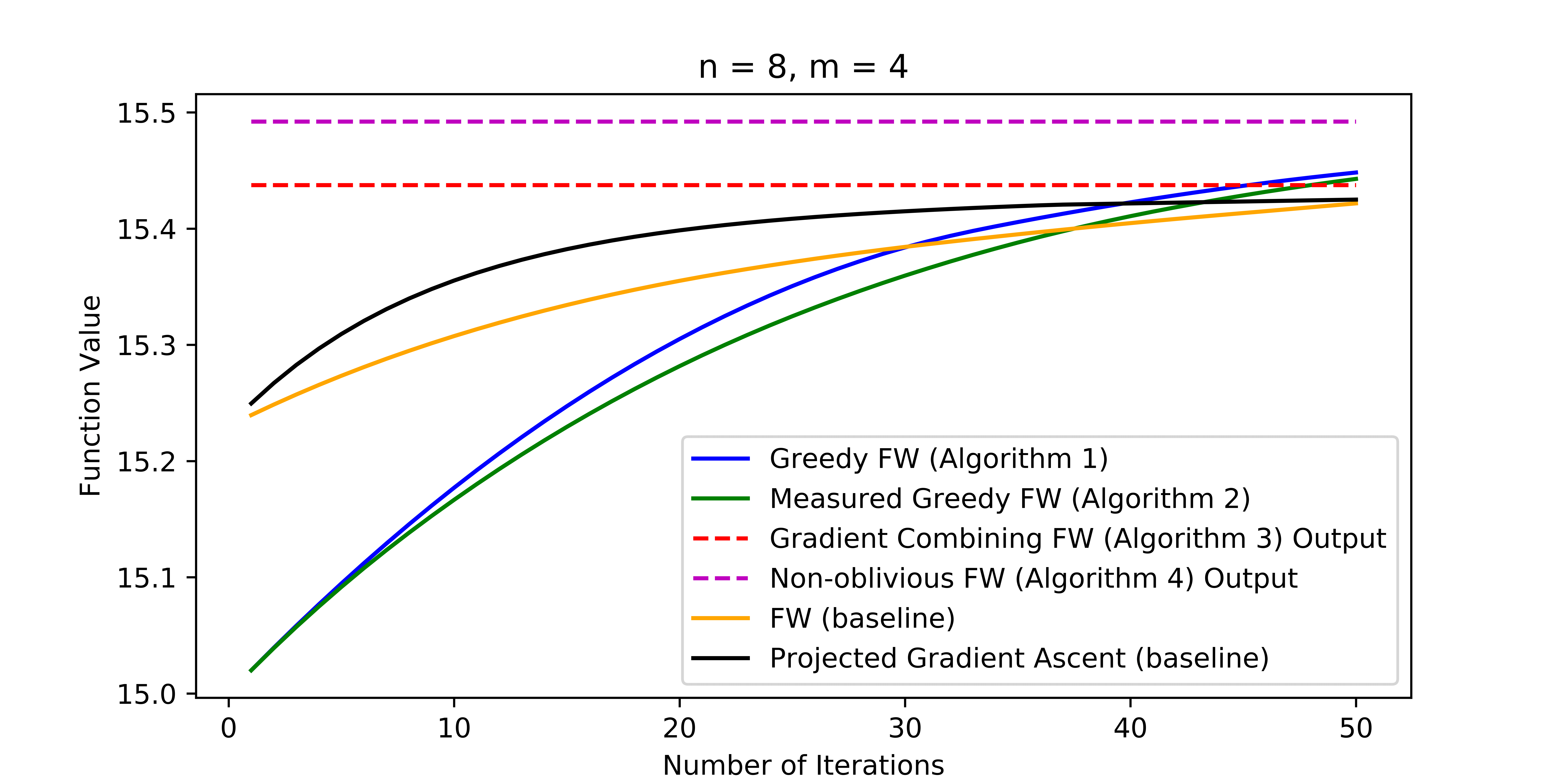
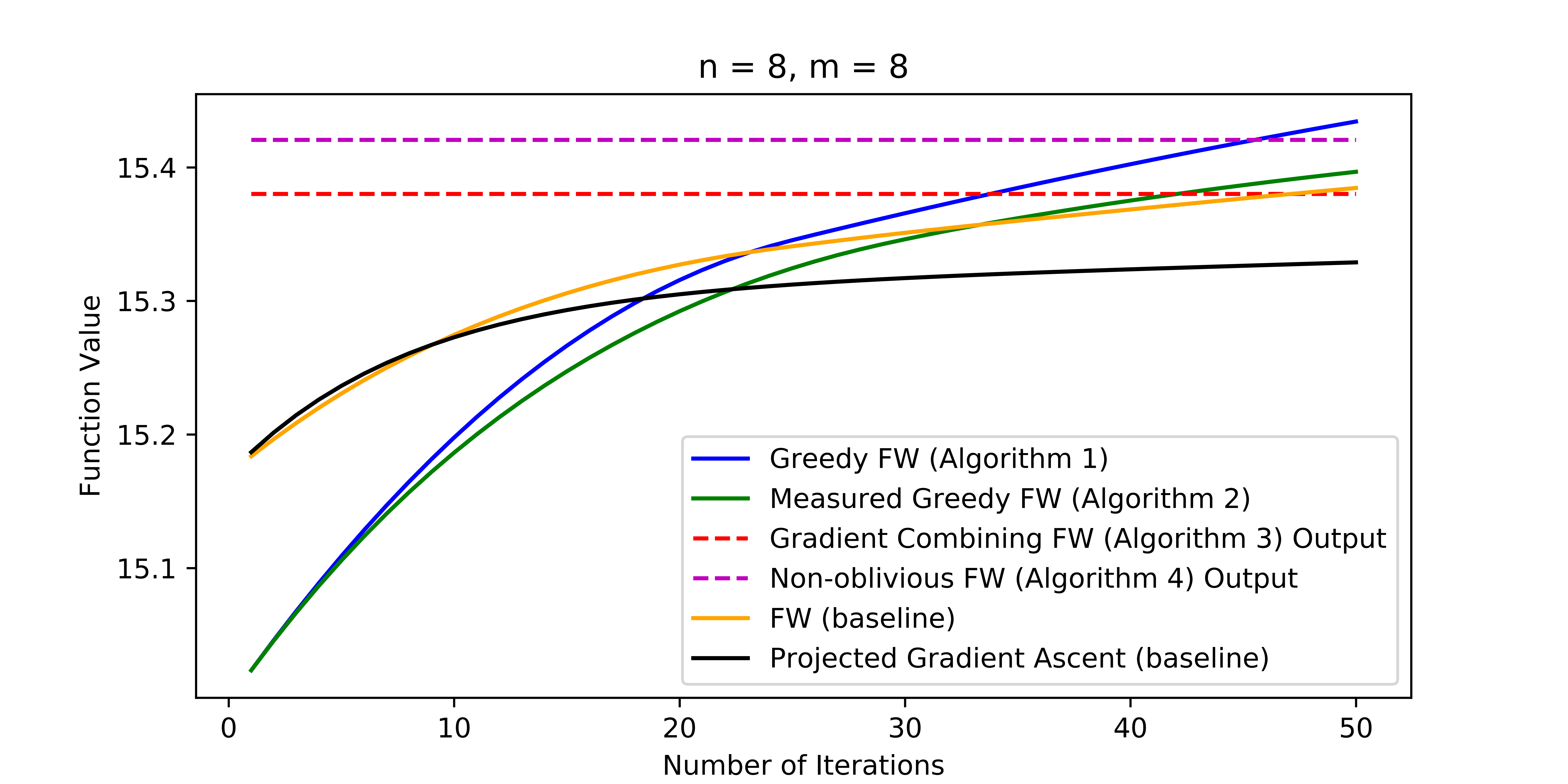
Refer to caption
(a) n=8,m=4formulae-sequence𝑛8𝑚4n=8,m=4
Refer to caption
(b) n=8,m=8formulae-sequence𝑛8𝑚8n=8,m=8
Refer to caption
(a) n=8,m=12formulae-sequence𝑛8𝑚12n=8,m=12
Refer to caption
(b) n=12,m=6formulae-sequence𝑛12𝑚6n=12,m=6
Refer to caption
(c) n=12,m=12formulae-sequence𝑛12𝑚12n=12,m=12
Refer to caption
(d) n=12,m=18formulae-sequence𝑛12𝑚18n=12,m=18
Refer to caption
(e) n=16,m=8formulae-sequence𝑛16𝑚8n=16,m=8
Refer to caption
(f) n=16,m=16formulae-sequence𝑛16𝑚16n=16,m=16
Refer to caption
(g) n=16,m=24formulae-sequence𝑛16𝑚24n=16,m=24
Refer to caption
(h) Final outputs for the D-optimal design problem.
Figure 4: All the plots except for 4(h) correspond to the quadratic programming experiment from Section 4.2.1. For these plots, the dimension (n𝑛n) and the number of constraints (m𝑚m) is mentioned below each plot. Plot 4(h) pertains to the D-optimal experimental design problem from Section 4.2.2.

References

  • Alieva et al. [2021] Ayya Alieva, Aiden Aceves, Jialin Song, Stephen Mayo, Yisong Yue, and Yuxin Chen. Learning to make decisions via submodular regularization. In International Conference on Learning Representations, 2021.
  • Allen-Zhu et al. [2019] Zeyuan Allen-Zhu, Yuanzhi Li, and Yingyu Liang. Learning and generalization in overparameterized neural networks, going beyond two layers. In Advances in Neural Information Processing Systems, 2019.
  • Anari et al. [2016] Nima Anari, Shayan Oveis Gharan, and Alireza Rezaei. Monte carlo markov chain algorithms for sampling strongly rayleigh distributions and determinantal point processes. In 29th Annual Conference on Learning Theory, 2016.
  • Arora et al. [2012] Sanjeev Arora, Rong Ge, Ravi Kannan, and Ankur Moitra. Computing a nonnegative matrix factorization – provably. In Proceedings of the Forty-Fourth Annual ACM Symposium on Theory of Computing, 2012.
  • Bian et al. [2017a] An Bian, Kfir Y. Levy, Andreas Krause, and Joachim M. Buhmann. Continuous dr-submodular maximization: Structure and algorithms. In Proceedings of the 31st International Conference on Neural Information Processing Systems, 2017a.
  • Bian et al. [2019] An Bian, Joachim M. Buhmann, and Andreas Krause. Optimal dr-submodular maximization and applications to provable mean field inference. In Proceedings of the 36th International Conference on Machine Learning, 2019.
  • Bian et al. [2017b] Andrew An Bian, Baharan Mirzasoleiman, Joachim M. Buhmann, and Andreas Krause. Guaranteed non-convex optimization: Submodular maximization over continuous domains. In AISTATS, 2017b.
  • Bresler et al. [2019] Guy Bresler, Frederic Koehler, Ankur Moitra, and Elchanan Mossel. Learning restricted boltzmann machines via influence maximization. In Proceedings of the 51st Annual ACM SIGACT Symposium on Theory of Computing, 2019.
  • Bubeck [2015] Sébastien Bubeck. Convex optimization: Algorithms and complexity. Found. Trends Mach. Learn., 2015.
  • Călinescu et al. [2011] Gruia Călinescu, Chandra Chekuri, Martin Pál, and Jan Vondrák. Maximizing a monotone submodular function subject to a matroid constraint. SIAM J. Comput., 2011.
  • Chen et al. [2018] Lin Chen, Hamed Hassani, and Amin Karbasi. Online continuous submodular maximization. In Proceedings of the Twenty-First International Conference on Artificial Intelligence and Statistics, 2018.
  • Chen et al. [2019a] Lin Chen, Moran Feldman, and Amin Karbasi. Unconstrained submodular maximization with constant adaptive complexity. In Proceedings of the 51st Annual ACM SIGACT Symposium on Theory of Computing, STOC 2019, 2019a.
  • Chen et al. [2019b] Yuxin Chen, Yuejie Chi, Jianqing Fan, and Cong Ma. Gradient descent with random initialization: fast global convergence for nonconvex phase retrieval. Mathematical Programming, 2019b.
  • Derezinski et al. [2020] Michal Derezinski, Feynman Liang, and Michael Mahoney. Bayesian experimental design using regularized determinantal point processes. In Proceedings of the Twenty Third International Conference on Artificial Intelligence and Statistics, 2020.
  • Djolonga and Krause [2014] Josip Djolonga and Andreas Krause. From map to marginals: Variational inference in bayesian submodular models. In Advances in Neural Information Processing Systems, 2014.
  • Du et al. [2019] Simon S. Du, Xiyu Zhai, Barnabas Poczos, and Aarti Singh. Gradient descent provably optimizes over-parameterized neural networks. In International Conference on Learning Representations, 2019.
  • Dwivedi et al. [2019] Raaz Dwivedi, Yuansi Chen, Martin J. Wainwright, and Bin Yu. Log-concave sampling: Metropolis-hastings algorithms are fast. Journal of Machine Learning Research, 2019.
  • Elenberg et al. [2016] Ethan R. Elenberg, Rajiv Khanna, Alexandros G. Dimakis, and Sahand Negahban. Restricted strong convexity implies weak submodularity. In Proceedings of the 30th Conference on Neural Information Processing Systems, 2016.
  • Elenberg et al. [2017] Ethan R. Elenberg, Alexandros G. Dimakis, Moran Feldman, and Amin Karbasi. Streaming weak submodularity: Interpreting neural networks on the fly. In Proceedings of the 31st International Conference on Neural Information Processing Systems, 2017.
  • Ene and Nguyen [2019] Alina Ene and Huy L. Nguyen. Parallel algorithm for non-monotone dr-submodular maximization. In Proceedings of the 37th International Conference on Machine Learning, 2019.
  • Ene et al. [2020] Alina Ene, Sofia Maria Nikolakaki, and Evimaria Terzi. Team formation: Striking a balance between coverage and cost. CoRR, 2020.
  • Feldman [2021] Moran Feldman. Guess free maximization of submodular and linear sums. Algorithmica, 2021.
  • Feldman et al. [2011] Moran Feldman, Joseph Naor, and Roy Schwartz. A unified continuous greedy algorithm for submodular maximization. In 2011 IEEE 52nd Annual Symposium on Foundations of Computer Science, 2011.
  • Filmus and Ward [2012] Yuval Filmus and Justin Ward. A tight combinatorial algorithm for submodular maximization subject to a matroid constraint. In 2012 IEEE 53rd Annual Symposium on Foundations of Computer Science, 2012.
  • Frank and Wolfe [1956] Marguerite Frank and Philip Wolfe. An algorithm for quadratic programming. Naval Research Logistics Quarterly, 1956.
  • Ge et al. [2015] Rong Ge, Furong Huang, Chi Jin, and Yang Yuan. Escaping from saddle points — online stochastic gradient for tensor decomposition. In Proceedings of The 28th Conference on Learning Theory, 2015.
  • Gillenwater et al. [2012] J. Gillenwater, A. Kulesza, and B. Taskar. Near-Optimal MAP Inference for Determinantal Point Processes. In Proc. Neural Information Processing Systems (NIPS), 2012.
  • Harshaw et al. [2019] Chris Harshaw, Moran Feldman, Justin Ward, and Amin Karbasi. Submodular maximization beyond non-negativity: Guarantees, fast algorithms, and applications. In ICML, 2019.
  • Hassani et al. [2017] Hamed Hassani, Mahdi Soltanolkotabi, and Amin Karbasi. Gradient methods for submodular maximization. In Proceedings of the 31st International Conference on Neural Information Processing Systems, 2017.
  • Hassani et al. [2020a] Hamed Hassani, Amin Karbasi, Aryan Mokhtari, and Zebang Shen. Stochastic conditional gradient++: (non)convex minimization and continuous submodular maximization. SIAM Journal on Optimization, 2020a.
  • Hassani et al. [2020b] Hamed Hassani, Amin Karbasi, Aryan Mokhtari, and Zebang Shen. Stochastic conditional gradient++, 2020b.
  • Hazan et al. [2016] Elad Hazan, Kfir Y. Levy, and Shai Shalev-Shwartz. On graduated optimization for stochastic non-convex problems. In Proceedings of The 33rd International Conference on Machine Learning, 2016.
  • He [2010] Xiaofei He. Laplacian regularized d-optimal design for active learning and its application to image retrieval. IEEE Transactions on Image Processing, 2010.
  • Jacot et al. [2018] Arthur Jacot, Franck Gabriel, and Clément Hongler. Neural tangent kernel: Convergence and generalization in neural networks. In Proceedings of the 32nd International Conference on Neural Information Processing Systems, 2018.
  • Kazemi et al. [2020a] Ehsan Kazemi, Shervin Minaee, Moran Feldman, and Amin Karbasi. Regularized submodular maximization at scale. CoRR, 2020a.
  • Kazemi et al. [2020b] Ehsan Kazemi, Shervin Minaee, Moran Feldman, and Amin Karbasi. Regularized submodular maximization at scale. CoRR, 2020b.
  • Kempe et al. [2003] David Kempe, Jon Kleinberg, and Éva Tardos. Maximizing the spread of influence through a social network. In Proceedings of the Ninth ACM SIGKDD International Conference on Knowledge Discovery and Data Mining, KDD ’03. Association for Computing Machinery, 2003.
  • Krause and Cevher [2010] Andreas Krause and Volkan Cevher. Submodular dictionary selection for sparse representation. In Proceedings of the 27th International Conference on International Conference on Machine Learning, 2010.
  • Kulesza [2012] Alex Kulesza. Determinantal point processes for machine learning. Foundations and Trends® in Machine Learning, 2012.
  • Lattimore and Szepesvari [2020] Tor Lattimore and Csaba Szepesvari. Bandit algorithms. Cambridge University Press, 2020.
  • Mirzasoleiman et al. [2013] Baharan Mirzasoleiman, Amin Karbasi, Rik Sarkar, and Andreas Krause. Distributed submodular maximization: Identifying representative elements in massive data. In Advances in Neural Information Processing Systems, 2013.
  • Mokhtari et al. [2018a] Aryan Mokhtari, Hamed Hassani, and Amin Karbasi. Conditional gradient method for stochastic submodular maximization: Closing the gap. In Proceedings of the Twenty-First International Conference on Artificial Intelligence and Statistics, 2018a.
  • Mokhtari et al. [2018b] Aryan Mokhtari, Hamed Hassani, and Amin Karbasi. Decentralized submodular maximization: Bridging discrete and continuous settings. In Proceedings of the 35th International Conference on Machine Learning, 2018b.
  • Murty and Kabadi [1987] K. G. Murty and S. N. Kabadi. Some np-complete problems in quadratic and nonlinear programming. Mathematical Programming, 1987.
  • Nesterov [2018] Yurii Nesterov. Lectures on Convex Optimization. Springer Publishing Company, Incorporated, 2018.
  • Netrapalli et al. [2014] Praneeth Netrapalli, U N Niranjan, Sujay Sanghavi, Animashree Anandkumar, and Prateek Jain. Non-convex robust pca. In Advances in Neural Information Processing Systems, 2014.
  • Niazadeh et al. [2018] Rad Niazadeh, Tim Roughgarden, and Joshua R. Wang. Optimal algorithms for continuous non-monotone submodular and dr-submodular maximization. In Proceedings of the 32nd International Conference on Neural Information Processing Systems, 2018.
  • Raut et al. [2021] Prasanna Sanjay Raut, Omid Sadeghi, and Maryam Fazel. Online dr-submodular maximization with stochastic cumulative constraints, 2021.
  • Rebeschini and Karbasi [2015] Patrick Rebeschini and Amin Karbasi. Fast mixing for discrete point processes. In Proceedings of The 28th Conference on Learning Theory, 2015.
  • Robinson et al. [2019] Joshua Robinson, Suvrit Sra, and Stefanie Jegelka. Flexible modeling of diversity with strongly log-concave distributions. In Advances in Neural Information Processing Systems, 2019.
  • Sadeghi and Fazel [2019] Omid Sadeghi and Maryam Fazel. Online continuous DR-submodular maximization with long-term budget constraints. In Proceedings of the Twenty Third International Conference on Artificial Intelligence and Statistics, 2019.
  • Sadeghi et al. [2020] Omid Sadeghi, Prasanna Raut, and Maryam Fazel. A single recipe for online submodular maximization with adversarial or stochastic constraints. In Advances in Neural Information Processing Systems, 2020.
  • Singla et al. [2014] Adish Singla, Ilija Bogunovic, Gábor Bartók, Amin Karbasi, and Andreas Krause. Near-optimally teaching the crowd to classify. In Proceedings of the 31st International Conference on International Conference on Machine Learning, 2014.
  • Staib and Jegelka [2017] Matthew Staib and Stefanie Jegelka. Robust budget allocation via continuous submodular functions. In Proceedings of the 34th International Conference on Machine Learning, 2017.
  • Sun et al. [2016] Ju Sun, Qing Qu, and John Wright. When are nonconvex problems not scary?, 2016.
  • Sun and Luo [2016] Ruoyu Sun and Zhi-Quan Luo. Guaranteed matrix completion via non-convex factorization. IEEE Transactions on Information Theory, 2016.
  • Sviridenko et al. [2017] Maxim Sviridenko, Jan Vondrák, and Justin Ward. Optimal approximation for submodular and supermodular optimization with bounded curvature. Math. Oper. Res., 2017.
  • Tohidi et al. [2020] Ehsan Tohidi, Rouhollah Amiri, Mario Coutino, David Gesbert, Geert Leus, and Amin Karbasi. Submodularity in action: From machine learning to signal processing applications. IEEE Signal Processing Magazine, 2020.
  • Wei et al. [2015] Kai Wei, Rishabh Iyer, and Jeff Bilmes. Submodularity in data subset selection and active learning. In Proceedings of the 32nd International Conference on International Conference on Machine Learning - Volume 37, 2015.
  • Wilder [2018a] Bryan Wilder. Risk-sensitive submodular optimization. Proceedings of the AAAI Conference on Artificial Intelligence, 2018a.
  • Wilder [2018b] Bryan Wilder. Equilibrium computation and robust optimization in zero sum games with submodular structure. Proceedings of the AAAI Conference on Artificial Intelligence, 2018b.
  • Xie et al. [2019] Jiahao Xie, Chao Zhang, Zebang Shen, Chao Mi, and Hui Qian. Decentralized gradient tracking for continuous dr-submodular maximization. In Proceedings of the Twenty-Second International Conference on Artificial Intelligence and Statistics, 2019.
  • Zhang et al. [2019] Mingrui Zhang, Lin Chen, Hamed Hassani, and Amin Karbasi. Online continuous submodular maximization: From full-information to bandit feedback. In Advances in Neural Information Processing Systems, 2019.