Fixed-Budget Best-Arm Identification in Structured Bandits
Abstract
Best-arm identification (BAI) in a fixed-budget setting is a bandit problem where the learning agent maximizes the probability of identifying the optimal (best) arm after a fixed number of observations. Most works on this topic study unstructured problems with a small number of arms, which limits their applicability. We propose a general tractable algorithm that incorporates the structure, by successively eliminating suboptimal arms based on their mean reward estimates from a joint generalization model. We analyze our algorithm in linear and generalized linear models (GLMs), and propose a practical implementation based on a G-optimal design. In linear models, our algorithm has competitive error guarantees to prior works and performs at least as well empirically. In GLMs, this is the first practical algorithm with analysis for fixed-budget BAI.
1 Introduction
Best-arm identification (BAI) is a pure exploration bandit problem where the goal is to identify the optimal arm. It has many applications, such as online advertising, recommender systems, and vaccine tests (Hoffman et al., 2014; Lattimore and Szepesvári, 2020). In fixed-budget (FB) BAI (Bubeck et al., 2009; Audibert et al., 2010), the goal is to accurately identify the optimal arm within a fixed budget of observations (arm pulls). This setting is common in applications where the observations are costly. However, it is more complex to analyze than the fixed-confidence (FC) setting, due to complications in budget allocation (Lattimore and Szepesvári, 2020, Section 33.3). In FC BAI, the goal is to find the optimal arm with a guaranteed level of confidence, while minimizing the sample complexity.
Structured bandits are bandit problems in which the arms share a common structure, e.g., linear or generalized linear models (Filippi et al., 2010; Soare et al., 2014). BAI in structured bandits has been mainly studied in the FC setting with the linear model (Soare et al., 2014; Xu et al., 2018; Degenne et al., 2020). The literature of FB BAI for linear bandits was limited to (Hoffman et al., 2014) for a long time. This algorithm does not explore sufficiently, and thus, performs poorly (Xu et al., 2018). Katz-Samuels et al. (2020) recently proposed for FB BAI in linear bandits. Although this algorithm has desirable theoretical guarantees, it is computationally intractable, and its approximation loses the desired properties of the exact form. - (Yang and Tan, 2021) is a concurrent work for FB BAI in linear bandits. It is a sequential halving algorithm with a special first stage, in which most arms are eliminated. This makes the algorithm inaccurate when the number of arms is much larger than the number of features, a common setting in structured problems. We discuss these three FB BAI algorithms in detail in Section 7 and empirically evaluate them in Section 8.
In this paper, we address the shortcomings of prior work by developing a general successive elimination algorithm that can be applied to several FB BAI settings (Section 3). The key idea is to divide the budget into multiple stages and allocate it adaptively for exploration in each stage. As the allocation is updated in each stage, our algorithm adaptively eliminates suboptimal arms, and thus, properly addresses the important trade-off between adaptive and static allocation in structured BAI (Soare et al., 2014; Xu et al., 2018). We analyze our algorithm in linear bandits in Section 4. In Section 5, we extend our algorithm and analysis to generalized linear models (GLMs) and present the first BAI algorithm for these models. Our error bounds in Sections 4 and 5 motivate the use of a G-optimal allocation in each stage, for which we derive an efficient algorithm in Section 6. Using extensive experiments in Section 8, we show that our algorithm performs at least as well as a number of baselines, including , , and -.
2 Problem Formulation
We consider a general stochastic bandit with arms. The reward distribution of each arm (the set of arms) has mean . Without loss of generality, we assume that ; thus arm 1 is optimal. Let be the feature vector of arm , such that holds, where is the -norm in . We denote the observed rewards of arms by . Formally, the reward of arm is , where is a -sub-Gaussian noise and is any function of , such that . In this paper, we focus on two instances of : linear (Eq. 1) and generalized linear (Eq. 4).
We denote by the fixed budget of arm pulls and by the arm returned by the BAI algorithm. In the FB setting, the goal is to minimize the probability of error, i.e., (Bubeck et al., 2009). This is in contrast to the FC setting, where the goal is to minimize the sample complexity of the algorithm for a given upper bound on .
3 Generalized Successive Elimination
Successive elimination (Karnin et al., 2013) is a popular BAI algorithm in multi-armed bandits (MABs). Our algorithm, which we refer to as Generalized Successive Elimination (), generalizes it to structured reward models . We provide the pseudo-code of in Algorithm 1.
operates in stages, where is a tunable elimination parameter, usually set to be 2. The budget is split evenly over stages, and thus, each stage has budget . In each stage , pulls arms for times and eliminates fraction of them. We denote the set of the remaining arms at the beginning of stage by . By construction, only a single arm remains after stages. Thus, and . In stage , performs the following steps:
Projection (Line 2): To avoid singularity issues, we project the remaining arms into their spanned subspace with dimensions. We discuss this more after Eq. 1.
Exploration (Line 3): The arms in are sampled according to an allocation vector , i.e., is the number of times that arm is pulled in stage . In Sections 4 and 5, we first report our results for general and then show how they can be improved if is an adaptive allocation based on the G-optimal design, described in Section 6.
Estimation (Line 4): Let and be the feature vectors and rewards of the arms sampled in stage , respectively. Given the reward model , , and , we estimate the mean reward of each arm in stage , and denote it by . For instance, if is a linear function, is estimated using linear regression, as in Eq. 1.
Elimination (Line 5): The arms in are sorted in descending order of , their top fraction is kept, and the remaining arms are eliminated.
At the end of stage , only one arm remains, which is returned as the optimal arm. While this algorithmic design is standard in MABs, it is not obvious that it would be near-optimal in structured problems, as this paper shows.
4 Linear Model
We start with the linear reward model, where , for an unknown reward parameter . The estimate of in stage is computed using least-squares regression as , where is the sample covariance matrix, and . This gives us the following mean estimate for each arm ,
| (1) |
The matrix is well-defined as long as spans . However, since eliminates arms, it may happen that the arms in later stages do not span . Thus, could be singular and would not be well-defined. We alleviate this problem by projecting111The projection can be done by multiplying the arm features with the matrix whose columns are the orthonormal basis of the subspace spanned by the arms (Yang and Tan, 2021). the arms in into their spanned subspace. We denote the dimension of this subspace by . Alternatively, we can address the singularity issue by using the pseudo-inverse of matrices (Huang et al., 2021). In this case, we remove the projection step, and replace with its pseudo-inverse.
4.1 Analysis
In this section, we prove an error bound for with the linear model. Although this error bound is a special case of that for GLMs (see Theorem 5.1), we still present it because more readers are familiar with linear bandit analysis than GLMs. To reduce clutter, we assume that all logarithms have base . We denote by , the sub-optimality gap of arm , and by , the minimum gap, which by the assumption in Section 2 is just .
Theorem 4.1.
with the linear model (Eq. 1) and any valid222Allocation strategy is valid if is invertible. allocation strategy identifies the optimal arm with probability at least for
| (2) |
where for any and matrix . If we use the G-optimal design (Algorithm 2) for , then
| (3) |
We sketch the proof in Section 4.2 and defer the detailed proof to Appendix A.
The error bound in (3) scales as expected. Specifically, it is tighter for a larger budget , which increases the statistical power of ; and a larger gap , which makes the optimal arm easier to identify. The bound is looser for larger and , which increase with the instance size; and larger reward noise , which increases uncertainty and makes the problem instance harder to identify. We compare this bound to the related works in Section 7.
There is no lower bound for FB BAI in structured bandits. Nevertheless, in the special case of MABs, our bound ((3)) matches the FB BAI lower bound in Kaufmann et al. (2016), up to a factor of . It also roughly matches the tight lower bound of Carpentier and Locatelli (2016), which is . To see this, note that and , when we apply to a -armed bandit problem.
4.2 Proof Sketch
The key idea in analyzing is to control the probability of eliminating the optimal arm in each stage. Our analysis is modular and easy to extend to other elimination algorithms. Let be the event that the optimal arm is eliminated in stage . Then, where is the complement of event . In Lemma 1, we bound the probability that a suboptimal arm has a higher estimated mean reward than the optimal arm. This is a novel concentration result for linear bandits in successive elimination algorithms.
Lemma 1.
In with the linear model of Eq. 1, the probability that any suboptimal arm has a higher estimated mean reward than the optimal arm in stage satisfies
This lemma is proved using an argument mainly driven from a concentration bound. Next, we use it in Lemma 2 to bound the probability that the optimal arm is eliminated in stage .
Lemma 2.
In with the linear model (Eq. 1), the probability that the optimal arm is eliminated in stage satisfies where and is a shorthand for event .
This lemma is proved by examining how another arm can dominate the optimal arm and using Markov’s inequality. Finally, we bound in Theorem 4.1 using a union bound. We obtain the second bound in Theorem 4.1 by the Kiefer-Wolfowitz Theorem (Kiefer and Wolfowitz, 1960) for the G-optimal design described in Section 6.
5 Generalized Linear Model
We now study FB BAI in generalized linear models (GLMs) (McCullagh and Nelder, 1989), where , where is a monotone function known as the mean function. As an example, in logistic regression. We assume that the derivative of the mean function, , is bounded from below, i.e., , for some and all . Here can be any convex combination of and its maximum likelihood estimate in stage . This assumption is standard in GLM bandits (Filippi et al., 2010; Li et al., 2017). The existence of can be guaranteed by performing forced exploration at the beginning of each stage with the sampling cost of (Kveton et al., 2020). As satisfies , it can be computed efficiently by iteratively reweighted least squares (Wolke and Schwetlick, 1988). This gives us the following mean estimate for each arm ,
| (4) |
5.1 Analysis
In Theorem 5.1, we prove similar bounds to the linear model. The proof and its sketch are presented in Appendix B. These are the first BAI error bounds for GLM bandits.
Theorem 5.1.
with the GLM (Eq. 4) and any valid identifies the optimal arm with probability at least for
| (5) |
If we use the G-optimal design (Algorithm 2) for , then
| (6) |
The error bounds in Theorem 5.1 are similar to those in the linear model (Section 4.1), since The only major difference is in factor , which is in the linear case. This factor arises because GLM is a linear model transformed through some non-linear mean function . When is small, can have flat regions, which makes the optimal arm harder to identify. Therefore, our GLM bounds become looser as decreases. Note that the bounds in Theorem 5.1 depend on all other quantities same as the bounds in Theorem 4.1 do.
The novelty in our GLM analysis is in how we control the estimation error of using our assumptions on the existence of . The rest of the proof follows similar steps to those in Section 4.2 and are postponed to Appendix B.
6 G-Optimal Allocation
The stochastic error bounds in (2) and (5) can be optimized by minimizing with respect to , in particular, with respect to . In each stage , let , where and . Then, optimization of is equivalent to solving . This leads us to the G-optimal design (Kiefer and Wolfowitz, 1960), which minimizes the maximum variance along all .
We develop an algorithm based on the Frank-Wolfe (FW) method (Jaggi, 2013) to find the G-optimal design. Algorithm 2 contains the pseudo-code of it, which we refer to as . The G-optimal design is a convex relaxation of the G-optimal allocation; an allocation is the (integer) number of samples per arm while a design is the proportion of for each arm. Defining , by Danskin’s theorem (Danskin, 1966), we know where . This gives us the derivative of the objective function so we can use it in a FW algorithm. In each iteration, first minimizes the 1st-order surrogate of the objective, and then uses line search to find the best step-size and takes a gradient step. After iterations, it extracts an allocation (integral solution) from using an efficient rounding procedure from Allen-Zhu et al. (2017), which we call it . This procedure takes budget , design , and returns an allocation .
In Appendix C, we show that the error bounds of Theorems 4.1 and 5.1 still hold for large enough , if we use Algorithm 2 to obtain the allocation strategy at the exploration step (Line 3 of Algorithm 1). This results in the deterministic bounds in (3) and (6) in these theorems.
7 Related Work
To the best of our knowledge, there is no prior work on FB BAI for GLMs and our results are the first in this setting. However, there are three related algorithms for FB BAI in linear bandits that we discuss them in detail here. Before we start, note that there is no matching upper and lower bound for FB BAI in any setting (Carpentier and Locatelli, 2016). However, in MABs, it is known that successive elimination is near-optimal (Carpentier and Locatelli, 2016).
(Hoffman et al., 2014) is a Bayesian version of the gap-based exploration algorithm in Gabillon et al. (2012). This algorithm models correlations of rewards using a Gaussian process. As pointed out by Xu et al. (2018), does not explore enough and thus performs poorly. In Section D.1, we show under few simplifying assumptions that the error probability of is at most . Our error bound in Eq. 3 is at most . Thus, it improves upon by reducing dependence on the number of arms , from linear to logarithmic; and on budget , from linear to constant. We provide a more detailed comparison of these bounds in Section D.1. Our experimental results in Section 8 support these observations and show that our algorithm always outperforms in the linear setting.
(Katz-Samuels et al., 2020) is mainly a FC BAI algorithm based on a transductive design, which is modified to be used in the FB setting. It minimizes the Gaussian-width of the remaining arms with a progressively finer level of granularity. However, cannot be implemented exactly because the Gaussian width does not have a closed form and is computationally expensive to minimize. To address this, Katz-Samuels et al. (2020) proposed an approximation to , which still has some computational issues (see Remark 2 and Section 8.1). The error bound for , although is competitive, only holds for a relatively large budget (Theorem 7 in Katz-Samuels et al. 2020). We discuss this further in Remark 1. Although the comparison of their bound to ours is not straightforward, we show in Section D.2 that each bound can be superior in certain regimes that depend mainly on the relation of and . In particular, we show two cases: (i) Based on few claims in Katz-Samuels et al. (2020) that are not rigorously proved (see (i) in Section D.2 for more details), their error bound is at most which is better than our bound (Eq. 2) only if . (ii) We can also show that their bound is at most under the G-optimal design, which is worse than our error bound (Eq. 3).
In our experiments with in Section 8, we implemented its approximation and it never performed better than our algorithm. We also show in Section 8.1 that approximate is much more computationally expensive compared to our algorithm.
- (Yang and Tan, 2021) uses a G-optimal design in a sequential elimination framework for FB BAI. In the first stage, it eliminates all the arms except . This makes the algorithm prone to eliminating the optimal arm in the first stage, especially when the number of arms is larger than . It also adds a linear (in ) factor to the error bound. In Section D.3, we provide a detailed comparison between the error bound of - and ours, and show that similar to the comparison with , there are regimes where each bound is superior. However, we show that our bound is tighter in the more practically relevant setting of . In particular, we show that their error is at most . Now assuming for some , if we divide our bound (Eq. 3) with theirs, we obtain which is less than 1, so in this case our error bound is tighter. However, for , their bound is tighter. Finally, we note that our experiments in Section 8 and Section E.3 support these observations.
8 Experiments
In this section, we compare to several baselines including all linear FB BAI algorithms: , , and -. Others are variants of cumulative regret (CR) bandits and FC BAI algorithms. For CR algorithms, the baseline stops at the budget limit and returns the most pulled arm.333In Appendix D, we argue that this is a reasonable stopping rule. We use (Li et al., 2010) and - (Li et al., 2017), which are the state-of-the-art for linear and GLM bandits, respectively. (a FC BAI algorithm) (Xu et al., 2018) is used with its stopping rule at the budget limit. We tune its using a grid search and only report the best result. In Appendix F, we derive proper error bounds for these baselines to further justify the variants.
The accuracy is an estimate of , as the fraction of Monte Carlo replications where the algorithm finds the optimal arm. We run with linear model and uniform exploration (-), with (--), with sequential G-optimal allocation of Soare et al. (2014) (--), and with Wynn’s G-optimal method (--). For Wynn’s method, see Fedorov (1972). We set in all experiments, as this value tends to perform well in successive elimination (Karnin et al., 2013). For , we evaluate the Greedy version (-) and show its results only if it outperforms . For -, see Xu et al. (2018). In each experiment, we fix , , or ; depending on the experiment to show the desired trend. Similar trends can be observed if we fix the other parameters and change these. For further detail of our choices of kernels for and also our real-world data experiments, see Appendix E.
8.1 Linear Experiment: Adaptive Allocation
We start with the example in Soare et al. (2014), where the arms are the canonical -dimensional basis plus a disturbing arm with . We set and . Clearly the optimal arm is , however, when the angle is as small as 1/10, the disturbing arm is hard to distinguish from . As argued in Soare et al. (2014), this is a setting where an adaptive strategy is optimal (see Section G.1 for further discussion on Adaptive vs. Static strategies).
Fig. 2 shows that -- is the second-best algorithm for smaller and the best for larger . - performs poorly here, and thus, we omit it. We conjecture that - fails because it uses Gaussian processes and there is a very low correlation between the arms in this experiment. wins mostly for smaller and loses for larger . This could be because its regret is linear in (Appendix D). has lower accuracy than several other algorithms. We could only simulate for , since its computational cost is high for larger values of . For instance, at , completes runs in seconds; while it only takes to seconds for the other algorithms. At , completes runs in hours (see Section E.1).
In this experiment, and both - and have stages and perform similarly. Therefore, we only report the results for . This also happens in Section 8.2.
8.2 Linear Experiment: Static Allocation
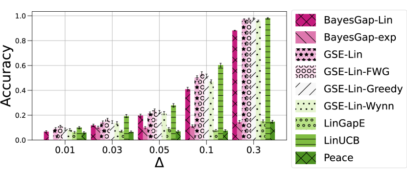
As in Xu et al. (2018), we take arms and , where and . In this experiment, knowing the rewards does not change the allocation strategy. Therefore, a static allocation is optimal (Xu et al., 2018). The goal is to evaluate the ability of the algorithm to adapt to a static situation.
Our results are reported in Fig. 1. We observe that performs the best when is small (harder instances). This is expected since suboptimal arms are well away from the optimal one, and CR algorithms do well in this case (Appendix D). Our algorithms are the second-best when is sufficiently large, converging to the optimal static allocation. -, , and cannot take advantage of larger , probably because they adapt to the rewards too early. This example demonstrates how well our algorithms adjust to a static allocation, and thus, properly address the tradeoff between static and adaptive allocation.
8.3 Linear Experiment: Randomized
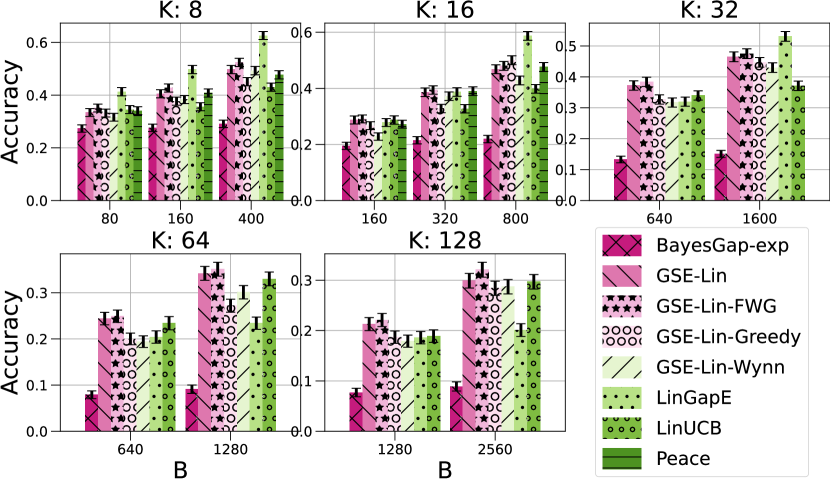
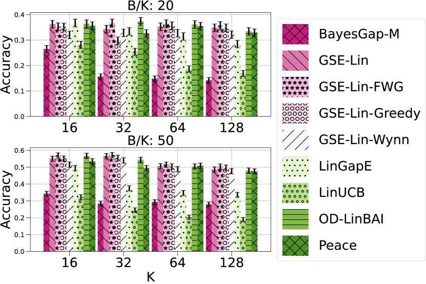
In this experiment, we use the example in Tao et al. (2018) and Yang and Tan (2021). For each bandit instance, we generate i.i.d. arms sampled from the unit sphere centered at the origin with . We let , where and are the two closest arms. As a consequence, is the optimal arm and is the disturbing arm. The goal is to evaluate the expected performance of the algorithms for a random instance to avoid bias in choosing the bandit instances.
We fix in Fig. 3 and compare the performance for different . -- has competitive performance with other algorithms. We can see that G-optimal policies have similar expected performance while is slightly better. Again, performance degrades as increases and underperforms our algorithms. Moreover, the performance of - worsens as increases, especially for . We report more experiments in this setting, comparing to -, in Section E.3.
8.4 GLM Experiment
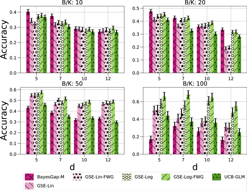
As an instance of GLM, we study a logistic bandit. We generate i.i.d. arms from uniform distribution on with , , and , where is a identity matrix. The reward of arm is defined as , where and is a Bernoulli distribution with mean . We use with a logistic regression model (-) and also with the linear models to evaluate the robustness of to model misspecification. For exploration, we only use (--), as it performs better than the other G-optimal allocations in earlier experiments. We also use a modification of - (Li et al., 2017), a state-of-the-art GLM CR algorithm, for FB BAI.
The results in Fig. 4 show with logistic models outperforms linear models, and improves on uniform exploration in the GLM case. These experiments also show the robustness of to model misspecification, since the linear model only slightly underperforms the logistic model. - results confirm that CR algorithms could fail in BAI. - falls short for ; the extra in their error bound also suggests failure for large . In contrast, the performance of keeps improving as increases.
9 Conclusions
In this paper, we studied fixed-budget best-arm identification (BAI) in linear and generalized linear models. We proposed the algorithm, which offers an adaptive framework for structured BAI. Our performance guarantees are near-optimal in MABs. In generalized linear models, our algorithm is the first practical fixed-budget BAI algorithm with analysis. Our experiments show the efficiency and robustness (to model misspecification) of our algorithm. Extending our algorithm to more general models could be a future direction (see Appendix H).
References
- Abbasi-yadkori et al. [2011] Yasin. Abbasi-yadkori, D. Pál, and C. Szepesvári. Improved algorithms for linear stochastic bandits. In Advances in Neural Information Processing Systems, pages 2312–2320, 2011.
- Allen-Zhu et al. [2017] Zeyuan Allen-Zhu, Yuanzhi Li, Aarti Singh, and Yining Wang. Near-optimal design of experiments via regret minimization. In International Conference on Machine Learning, pages 126–135, 2017.
- Audibert et al. [2010] Jean-Yves Audibert, Sébastien Bubeck, and Rémi Munos. Best Arm Identification in Multi-Armed Bandits. In Proceedings of the 23th Conference on Learning Theory, 2010.
- Berthet and Perchet [2017] Quentin Berthet and Vianney Perchet. Fast rates for bandit optimization with upper-confidence frank-wolfe. In I. Guyon, U. V. Luxburg, S. Bengio, H. Wallach, R. Fergus, S. Vishwanathan, and R. Garnett, editors, Advances in Neural Information Processing Systems, volume 30. Curran Associates, Inc., 2017.
- Bubeck et al. [2009] Sébastien Bubeck, Rémi Munos, and Gilles Stoltz. Pure exploration in multi-armed bandits problems. In International conference on Algorithmic learning theory, pages 23–37, 2009.
- Carpentier and Locatelli [2016] Alexandra Carpentier and Andrea Locatelli. Tight (lower) bounds for the fixed budget best arm identification bandit problem. In Conference on Learning Theory, pages 590–604, 2016.
- Damla Ahipasaoglu et al. [2008] Selin Damla Ahipasaoglu, Peng Sun, and Michael J Todd. Linear convergence of a modified Frank–Wolfe algorithm for computing minimum-volume enclosing ellipsoids. Optimization Methods and Software, 23(1):5–19, 2008.
- Danskin [1966] John M. Danskin. The theory of max-min, with applications. SIAM Journal on Applied Mathematics, 14(4):641–664, 1966.
- Degenne et al. [2019] Rémy Degenne, Wouter M Koolen, and Pierre Ménard. Non-asymptotic pure exploration by solving games. In H. Wallach, H. Larochelle, A. Beygelzimer, F. d'Alché-Buc, E. Fox, and R. Garnett, editors, Advances in Neural Information Processing Systems, volume 32. Curran Associates, Inc., 2019.
- Degenne et al. [2020] Rémy Degenne, Pierre Ménard, Xuedong Shang, and Michal Valko. Gamification of pure exploration for linear bandits. In International Conference on Machine Learning, pages 2432–2442, 2020.
- Fedorov [1972] Valerii Vadimovich Fedorov. Theory of Optimal Experiments. Probability and Mathematical Statistics. Academic Press, 1972.
- Filippi et al. [2010] Sarah Filippi, Olivier Cappe, Aurélien Garivier, and Csaba Szepesvári. Parametric bandits: The generalized linear case. In Advances in Neural Information Processing Systems, 2010.
- Gabillon et al. [2012] Victor Gabillon, Mohammad Ghavamzadeh, and Alessandro Lazaric. Best arm identification: A unified approach to fixed budget and fixed confidence. In Advances in Neural Information Processing Systems, pages 3212–3220, 2012.
- Hoffman et al. [2014] Matthew Hoffman, Bobak Shahriari, and Nando Freitas. On correlation and budget constraints in model-based bandit optimization with application to automatic machine learning. In Artificial Intelligence and Statistics, pages 365–374, 2014.
- Huang et al. [2021] Ruiquan Huang, Weiqiang Wu, Jing Yang, and Cong Shen. Federated linear contextual bandits. Advances in Neural Information Processing Systems, 34, 2021.
- Jaggi [2013] Martin Jaggi. Revisiting Frank-Wolfe: Projection-free sparse convex optimization. In International Conference on Machine Learning, pages 427–435, 2013.
- Jedra and Proutiere [2020] Yassir Jedra and Alexandre Proutiere. Optimal best-arm identification in linear bandits. In Advances in Neural Information Processing Systems, pages 10007–10017, 2020.
- Karnin et al. [2013] Zohar Karnin, Tomer Koren, and Oren Somekh. Almost optimal exploration in multi-armed bandits. In Proceedings of the 30th International Conference on International Conference on Machine Learning, page 1238–1246, 2013.
- Katz-Samuels et al. [2020] Julian Katz-Samuels, Lalit Jain, Zohar Karnin, and Kevin Jamieson. An empirical process approach to the union bound: Practical algorithms for combinatorial and linear bandits. In Advances in Neural Information Processing Systems, pages 10371–10382, 2020.
- Kaufmann et al. [2016] Emilie Kaufmann, Olivier Cappé, and Aurélien Garivier. On the complexity of best-arm identification in multi-armed bandit models. The Journal of Machine Learning Research, 17(1):1–42, 2016.
- Khachiyan [1996] Leonid G Khachiyan. Rounding of polytopes in the real number model of computation. Mathematics of Operations Research, 21(2):307–320, 1996.
- Kiefer and Wolfowitz [1960] Jack Kiefer and Jacob Wolfowitz. The equivalence of two extremum problems. Canadian Journal of Mathematics, 12:363–366, 1960.
- Kumar and Yildirim [2005] Piyush Kumar and E Alper Yildirim. Minimum-volume enclosing ellipsoids and core sets. Journal of Optimization Theory and Applications, 126(1):1–21, 2005.
- Kveton et al. [2020] Branislav Kveton, Manzil Zaheer, Csaba Szepesvari, Lihong Li, Mohammad Ghavamzadeh, and Craig Boutilier. Randomized exploration in generalized linear bandits. In International Conference on Artificial Intelligence and Statistics, pages 2066–2076, 2020.
- Lattimore and Szepesvári [2020] Tor Lattimore and Csaba Szepesvári. Bandit Algorithms. Cambridge University Press, 2020.
- Li et al. [2010] Lihong Li, Wei Chu, John Langford, and Robert E Schapire. A contextual-bandit approach to personalized news article recommendation. International Conference on World Wide Web, 2010.
- Li et al. [2017] Lihong Li, Yu Lu, and Dengyong Zhou. Provably optimal algorithms for generalized linear contextual bandits. In International Conference on Machine Learning, pages 2071–2080, 2017.
- McCullagh and Nelder [1989] Peter McCullagh and John A Nelder. Generalized Linear Models. Chapman & Hall, 1989.
- Riquelme et al. [2018] Carlos Riquelme, George Tucker, and Jasper Snoek. Deep bayesian bandits showdown: An empirical comparison of bayesian deep networks for Thompson sampling. In International Conference on Learning Representations, 2018.
- Soare et al. [2014] Marta Soare, Alessandro Lazaric, and Rémi Munos. Best-arm identification in linear bandits. In Advances in Neural Information Processing Systems, pages 828–836, 2014.
- Tao et al. [2018] Chao Tao, Saúl Blanco, and Yuan Zhou. Best arm identification in linear bandits with linear dimension dependency. In International Conference on Machine Learning, pages 4877–4886, 2018.
- Tripuraneni et al. [2021] Nilesh Tripuraneni, Chi Jin, and Michael Jordan. Provable meta-learning of linear representations. In International Conference on Machine Learning, pages 10434–10443, 2021.
- Vershynin [2019] Roman Vershynin. High-Dimensional Probability: An Introduction with Applications in Data Science. Cambridge Series in Statistical and Probabilistic Mathematics, 2019.
- Wolke and Schwetlick [1988] Robert. Wolke and Hartmut Schwetlick. Iteratively reweighted least squares: algorithms, convergence analysis, and numerical comparisons. SIAM Journal on Scientific and Statistical Computing, 9(5):907–921, 1988.
- Xu et al. [2018] Liyuan Xu, Junya Honda, and Masashi Sugiyama. A fully adaptive algorithm for pure exploration in linear bandits. In International Conference on Artificial Intelligence and Statistics, pages 843–851, 2018.
- Yang and Tan [2021] Junwen Yang and Vincent YF Tan. Towards minimax optimal best arm identification in linear bandits. arXiv preprint arXiv:2105.13017, 2021.
Appendix A Linear Model Proofs
We let for some integer so . This is for ease of reading in the analysis and proofs. We can deal with the cases in which is not an integer using rounding operators.
Proof of Lemma 1.
Fix stage . Since is fixed, we drop it in the rest of the proof. We start with
| (7) | ||||
| (8) |
Now since are independent, mean zero, -sub-Gaussian random variables, if we define
then by Hoeffding’s inequality (Theorem 2.6.3 in [Vershynin, 2019]) we can write and bound Eq. 8 as follows
| (9) |
It is important that the noise and features are independent. This is how we do not need adaptivity in each stage. Now since
We can bound Eq. 9 as follows
∎
Proof of Lemma 2.
Here we want to bound . Let denote the number of arms in whose is larger than . Then by Lemma 1, we have
Now Markov inequality gives
∎
Proof of Theorem 4.1.
By Lemma 2 the optimal arm is eliminated in one of the stages with probability at most
where we used Cauchy-Schwarz and Triangle inequality in the last inequality. Now by Kiefer-Wolfowitz Theorem [Kiefer and Wolfowitz, 1960], we know that under the G-optimal or D-optimal design
Therefore, and
| (10) |
∎
Appendix B GLM Proofs
The novelty in our GLM analysis is in how we control the estimation error of using our assumptions on the existence of . The rest of the proof follows similar steps to those in the linear model. The key idea is to obtain error bounds in each stage. First, in Lemma 1, we bound the probability that a suboptimal arm has a higher estimated mean reward than the optimal arm.
Lemma 1.
In with the GLM of Eq. 4, the probability that any suboptimal arm has a higher estimated mean reward than the optimal arm in stage satisfies
We prove this lemma using the assumption on and Hoeffding’s inequality.
Proof of Lemma 1.
Since is fixed we drop it in the rest of this proof. Let
where is some convex combination of and then
Note that we use for the gap before the mean function transformation. In the last inequality, we used Lemma 1 in [Kveton et al., 2020]. Now if we define
then by Hoeffding’s inequality, we get
Since is not known in the process, we need to dig deeper. By assumption, we know for some and for all , therefore by definition of , and
so
∎
Next, we bound the error probability at each stage in Lemma 2.
Lemma 2.
In with the GLM of Eq. 4, the probability that the optimal arm is eliminated in stage satisfies
Finally, we bound the probability of error and conclude the proof of Theorem 5.1 by using this result together with a union bound and the Kiefer-Wolfowitz Theorem.
Proof of Theorem 5.1.
By Lemma 2 we know that the optimal arm is eliminated in one of the stages with a probability that satisfies
Now by the Kiefer-Wolfowitz Theorem in [Kiefer and Wolfowitz, 1960], we know under the G-optimal or D-optimal design, so with this design we have
∎
Appendix C Frank Wolfe G-optimal Design
In this section, we develop more details for our FW G-optimal algorithm. Let be a distribution on , so . For instance, based on Kiefer and Wolfowitz [1960] (or Theorem 21.1 (Kiefer–Wolfowitz) and equation 21.1 from Lattimore and Szepesvári 2020) we should sample arm in stage , times, in which
where and we know that by the same Theorem. Finding is a convex problem for finite number of arms and can be solved using Frank-Wolfe algorithm (read note 3 from section 21 in Lattimore and Szepesvári 2020). After we get the optimal design , we can get the optimal allocation using a randomized rounding. There are algorithms that avoid randomized rounding by starting with an allocation problem (see Section 7). We develop yet another efficient algorithm for the optimal design in Section 6.
Khachiyan in Khachiyan [1996] showed that if we run the FW algorithm for iterations, we get , where is the FW solution. More precisely, we get the following error bounds as a corollary.
Corollary 1.
If we use with for Exploration, for iterations, then
Proof.
Also, Kumar and Yildirim [2005] suggested an initialization of the FW algorithm which achieves a bound independent of the number of arms. In particular, we get the following corollary.
Corollary 2.
If we use the using FW algorithm to find a G-optimal design with iterations starting from the initialization advised in Kumar and Yildirim [2005], then the accuracy is lower bounded as below;
Proof.
The same sort of Corollaries hold for GLM as well by starting from Theorem 5.1.
It is worth noting that based on the connection between D-optimal and G-optimal through the Kiefer-Wolfowitz Theorem [Kiefer and Wolfowitz, 1960], we can also look at the FW algorithm for a D-optimal allocation. In D-optimal design, we seek to minimize which is equal to minimizing and we get
We can use this in algorithm to implement the D-optimal allocation. The experimental results show similar performance using both G and D optimal allocation.
Appendix D Error Bound Comparison
In this section, we compare our analytical bounds to those in the related works. We try to derive similar bounds from their performance guarantee so that it is comparable to ours.
D.1 BayesGap
Based on Theorem 1 in Hoffman et al. [2014] we know if then simple regret has the following bound for any
where and . We use the following assumptions to transform the bounds in way comparable to our bounds. Namely we use where is a very small positive number and for simplicity we assume . We know that where . In this setting, the error bound satisfy the following
| (11) |
This bound is comparable to our bounds in Theorem 4.1. With the same assumptions, the error (regret) bound of with G-optimal design is
| (12) |
Comparing Eq. 11 and Eq. 12 we can see the improvements that has over . In terms of , we improve the linear dependence to log factors while in , we improve by eliminating the linear factor to the constant outside of the exponent.
In summary, We know for , while satisfies . The improvements in its dependence on and are obvious.
D.2 Peace
We compare our error bound Eq. 2 (or Eq. 3) to the performance guarantee of FB Peace in Theorem 7 of Katz-Samuels et al. [2020]. We consider different cases and claims as follows, however, it is not easy to compare our bounds to bounds since their bounds are defined using quite different approaches.
(i) If we accept few claims in the Peace paper (see below), their error bound is as follows:
which is better than our error bound Eq. 2 if , and worse otherwise.
Proof.
The error bound for in Theorem 7 of Katz-Samuels et al. [2020] is as follows;
| (13) |
for where is the set of all arms , is a constant and
with being a probability simplex and is any subset of arms, and i.e. . Also
where
| (14) |
where
By Proposition 1 in Katz-Samuels et al. [2020], we know since . This claim is not proved in Katz-Samuels et al. [2020] though. As such we can give advantage to and assume the bound Eq. 13 is rather
where we used Eq. 14 in the last inequality. By the claim after Theorem 7 in Katz-Samuels et al. [2020] for linear bandits. This claim is not proved in Katz-Samuels et al. [2020] neither. Now the bound is
Bringing all the elements to the exponent, this is of order
| (15) |
while Eq. 2 is
| (16) |
as such the comparison boils down to comparing
. Therefore, Eq. 15 is better than Eq. 16 if and worse otherwise. ∎
(ii) We can also show that their bound is
under the G-optimal design, which is worse than our error bound Eq. 3.
Proof.
On the other hand, by definition of we know
| (17) |
Also by Proposition 1 in Katz-Samuels et al. [2020] so we can rewrite Eq. 13 as
which under G-optimal design is
Now we can compare this with Eq. 3 and notice the extra in the exponent of bound. Again this can be written orderwise as
which by Eq. 16 the comparison simplifies to
which is always in the favor of our algorithm. ∎
Remark 1 (Budget Requirement of ).
Similar to above, using Proposition 1 and the claims in Katz-Samuels et al. [2020], for the lower bound required for budget we have
wherein the second inequality we used the claim that so we used to account for that.
Remark 2 (Implementational Issues of the Approximation for Peace).
We note that the “Computationally Efficient Algorithm for Combinatorial Bandits” in the Peace paper is proposed for the FC setting and it is not easy to derive it for the FB setting. Nonetheless, it still has some computational issues. To name a few, consider the calculating the gradient in estimateGradient subroutine, Algorithm 8 which could be cumbersome as it is done times. Also the maximization in subroutine, could be hard to track since the geometric properties of come into play.
D.3 OD-LinBAI
Here we compare the error upper bounds of our algorithm with OD-LinBAI. We show that their bound could simplify to
Now assume for some , if we divide our bound Eq. 3 with theirs we get
| (18) |
which is less than 1 and in this case our error bound is tighter. Nevertheless, in the case of , their bound is tighter.
Proof.
Our error bound for the linear case is (with and )
while the error bound of OD-LinBAI in theorem 2 is
where and
Thus their bound is
In the case when and is large, e.g. when for some , the top gaps would be approximately equal and we can roughly claim . Substituting these in the above error bound of OD-LinBAI yields
where we assumed a smaller upper bound for - in its favor. Now if we divide our bound with theirs we get
which is less than 1 and in this case our error bound is tighter. Nevertheless, in the case of , it seems their bound is tighter. ∎
Corner cases:
There are special corner cases where digging into different cases of our bounds we can compare them based on Eq. 18. We can see that our error bound is worse than OD-LinBAI in a particular setting where is small, is fixed, and . However, in the same setting, if , then the conclusion would be the opposite. We also list below several additional cases where our bound improves upon OD-LinBAI:
-
1.
is fixed, is fixed, and .
-
2.
is fixed, and .
-
3.
, while is small and is fixed (the case we described above).
-
4.
while is fixed, and grows at the same rate as . In this case, the term with grows faster than the exponent, because .
Appendix E More Experiments
First note that we set in the experiments and in the paper for ease of reading, but note that if we set such that the error bound in Eq. 3 is
which could be order-wise better than Eq. 3 under a specific regime of and . The problem is this would make the algorithm totally static and the adaptivity is lost and deteriorates the performance in instances like Section 8.1. As such, there is a trade-off and seems the best for adaptive experiments.
E.1 Details of the Experimental Results
Our preliminary experiments showed that is sensitive to the choice of the kernel. Therefore, we tune in each experiment and choose the best kernel from a set of kernels. Note that this gives an advantage. The best performing kernels are linear, exponential, and Matérn kernels. - stands for the linear, - for the exponential, and - for the Matérn kernels.
We used a combination of computing resources. The main resource we used is the USC Center for Advanced Research Computing (https://carc.usc.edu/). Their typical compute node has dual 8 to 16 core processors and resides on a 56 gigabit FDR InfiniBand backbone, each having 16 GB memory. We also used a PC with 16 GB memory and Intel(R) Core(TM) i7-10750H CPU. For the runs we even tried Google Cloud c2-standard-60 instances with 60 CPUs and 240 GB memory.
E.2 Real-World Data Experiments
For this experiment, we use the ”Automobile Dataset”444J. Schlimmer, Automobile Dataset, https://archive.ics.uci.edu/ml/datasets/Automobile, accessed: 01.05.2021, 1987 , which has features of different cars and their prices. We assume the car prices are not readily in hand, rather we get samples of them where the price of car is where is the price of car in the dataset. The dataset includes cars and we use the most informative subset of features namely ‘curb weight‘, ‘width‘, ‘engine size‘, ‘city mpg‘, and ‘highway mpg‘ so . All the features are rescaled to . We want to find the most expensive car by sampling. In each replication, we sample cars and run the algorithms with the given budget on them. The purpose is to evaluate the performance of the algorithms on a real-world dataset and test their robustness to model misspecification.
The other dataset is the ”Electric Motor temperature”555J. Bocker, Electric Motor Temperature, https://www.kaggle.com/wkirgsn/electric-motor-temperature, 2019, accessed: 01.05.2021 and we want to find the highest engine temperature. Again, we take samples from the temperature distribution where is the temperature of motor in the dataset. All the features are rescaled to [0,1] and is 11. The dataset includes data points.
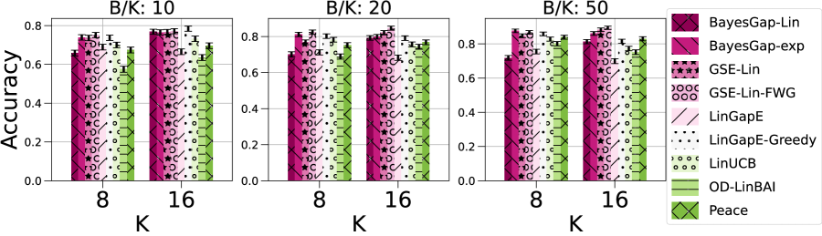
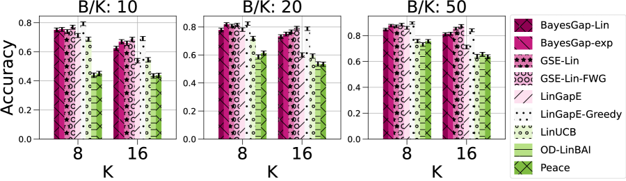
Fig. 5 and Fig. 5 show the results indicating variants outperform others or have competing performance with -. The experimental results in Fig. 5 show that our algorithm has the highest accuracy in most of the cases despite the fact that we use a linear model for a real-world dataset. This experiment also shows how well all the linear BAI algorithms could generalize to real-world situations.
E.3 More OD-LinBAI Experiments
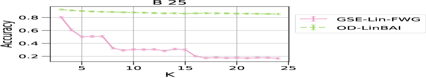
In this section, we include further experiments to compare with -. First, we illustrate that our algorithm outperforms - [Yang and Tan, 2021]. Fig. 6 shows the results for the same experiment as in Section 8.3 but with (to imitate Yang and Tan [2021]) for different and . We can observe for small budgets increasing our algorithm outperforms - more and more. While if is extremely large like we can see - outperform .

Fig. 7 shows the corner case experiment of Section 5.1 in Yang and Tan [2021] where , , , , and for where are i.i.d. samples. In this experiment - outperforms our algorithm. Since - only has 1 stage and simplifies to a G-optimal design, it seems that the specific setting of this experiment makes a G-optimal design most effective in only 1 stage.
Appendix F Cumulative Regret and Fixed-Confidence Baselines
By Proposition 33.2 in Lattimore and Szepesvári [2020] there is a connection between the policies designed for minimizing the cumulative regret and BAI policies. However, by the discussion after corollary 33.2 in Lattimore and Szepesvári [2020] the cumulative regret algorithms could under-perform for BAI depending on the bandit instance. This is because these algorithms mostly sample the optimal arm and play suboptimal arms barely enough to ensure they are not optimal. In BAI, this leads to a highly suboptimal performance with asymptotically polynomial simple regret. However, we can compare our BAI algorithm with cumulative regret bandit algorithms as a sanity check or potential competitor. We modify the cumulative regret algorithms into a BAI using a heuristic recommendation policy, mainly by returning the most frequently played arm.
We take algorithm [Li et al., 2010] and let be the pulled arm in stage , and let the number of stages be equal . has the following upper bound on its expected -stage regret. With probability at least ,
where hides additional log factors in [Li et al., 2010]. Note that this is a high-probability guarantee on the near-optimality of the average of played arms, the average feature vectors of all pulled arms. If we let this gap be smaller that then we get an error bound of
In a finite arm case, like our setting, we take the most frequently played arm, call it , as the optimal arm. The reason is that a cumulative regret algorithm plays the potentially optimal arm the most. We conjecture this is the same as the average of played arms, since when we have large enough budget the mode (i.e. ) converges to the mean by the Central Limit Theorem. If we set then which is of same order (except we get instead of which is better) as our bound in Theorem 4.1 also we used here.
For the GLM case, we employ - algorithm [Li et al., 2017] which improves the results of GLM-UCB [Filippi et al., 2010]. According to their most optimistic bound in Theorem 4 of Li et al. [2017], we know the - cumulative regret is less than for samples, where lower bounds the local behavior of near and is a positive universal constant. Now since simple regret is upper bounded by the cumulative regret, this is also a simple regret bound if we return , i.e.
Now if we set this expression equal we have
which is comparable to the bound in Theorem 5.1 but has a slower decrease in .
We could also turn an FC BAI algorithm into a FB algorithm by stopping at the budget limit and using their recommendation rule. We do a grid search and use the best for them. algorithm [Xu et al., 2018] is the state-of-art algorithm that performs the best among many [Degenne et al., 2020]. By their Theorem 2, we require access to to access the bound and find a proper for a given . This is not very desirable from a practical point of view since we need to know and beforehand. As such, in our experiments, we find the best by a grid search based on the empirical performance of the algorithm for FB BAI. We chose the best one for them in their favor.
Appendix G More on Related Work
G.1 Adaptive vs. Static BAI
As argued in Soare et al. [2014] and Xu et al. [2018], adaptive allocation is necessary for achieving optimal performance. However, it adds an extra factor to the confidence bounds, and worsens the sample complexity. Soare et al. [2014] and [Xu et al., 2018] propose their FC BAI algorithms -adaptive and LinGapE as an attempt to address this issue. Unlike -adaptive, LinGapE uses a transductive design and is shown to outperform -adaptive. Our algorithm with G-optimal design applies an optimal allocation within each phase, which is different than the greedy and static allocation used by -adaptive. We modify LinGapE to be applied to the FB BAI setting and compare it with our algorithm in Section 8. In most cases, our algorithm performed better. Therefore, we believe our algorithm is capable of properly balancing the trade-off between adaptive and static allocations. We further discuss the related work, such as those in the FC BAI setting and optimal design in Appendix G.
G.2 BAI with Successive Elimination
Successive elimination [Karnin et al., 2013] is common in BAI; Sequential Halving from Karnin et al. [2013] is closely related to our work which is developed for the FB MAB problems. We extend these algorithms to the structured bandits and use an optimal static stage which adapts to the rewards between the stages.
G.3 Optimal Design
Finding the optimal distribution over arms is ”optimal design” while finding the optimal number of samples per arm is called ”optimal allocation”. The exact optimization for many design problems is NP-Hard [Allen-Zhu et al., 2017] Therefore, in the BAI literature, optimal allocation is usually treated as an implementation detail [Soare et al., 2014; Degenne et al., 2020]. and several heuristics are proposed [Khachiyan, 1996; Kumar and Yildirim, 2005]. However, most of these methods are greedy [Degenne et al., 2020]; in particular, they start with one observation per arm, and then continue with the arm that reduces the uncertainty the most in some sense [Soare et al., 2014]. Jedra and Jedra and Proutiere [2020] have a procedure (Lemma 5) that does not start with a sample for each arm but it works for FC setting. Tao et al. [2018] suggest that solving the convex relaxation of the optimal design along with a randomized estimator yields a better solution than the greedy methods. This motivates our algorithm, which is based on FW fast-rate algorithms. Berthet and Perchet [2017] developed a UCB Frank-Wolfe method for bandit optimization. Their goal is to maximize an unknown smooth function with fast rates. Simple regret could be a special case of their framework, however, as of now, it is not clear how to use this method for a BAI bandit problem [Degenne et al., 2019]. In our experiments, we tried several variants of optimal design techniques where the results confirm that mostly outperforms the others.
G.4 Related Work on Fixed-Confidence Best Arm Identification
In this section, we discuss the works related to the FC setting in more detail. There are several BAI algorithms for linear bandits under the FC setting. We only discuss the main algorithms. Soare et al. [2014] proposed the algorithms based on transductive experimental design [Xu et al., 2018]. In the static case, they fix all arm selections before observing any reward; as a result, it cannot estimate the near-optimal arms. The remedy is an algorithm that adapts the sampling based on the rewards history to assign most of the budget on distinguishing between the suboptimal arms. Abbasi-yadkori et al. [2011] introduced a confidence bound based on Azuma’s inequality for adaptive strategies which is looser than the static bounds by a factor. The -adaptive is trying to avoid the extra factor as a semi-adaptive algorithm. This algorithm improves the sample complexity in theory, but the algorithm must discard the history of previous phases to apply the bounds. This empirically degrades the performance as shown in Xu et al. [2018].
Xu et al. [2018] proposed the algorithm which avoids the factor by careful construction of the confidence bounds. However, the sample complexity of their algorithm is linear in , which is not desirable. In this paper, we derive error bounds logarithmic in for both linear and generalized linear models.
Jedra and Proutiere [2020] introduced an FC BAI algorithm which tracks an optimal proportion of arm draws and updates these proportions as rarely as possible to avoid compromising its theoretical guarantees. Lemma 5 in this paper provides a procedure that can help avoid greedy sampling of all the arms.
Appendix H Heuristic Exploration for More General Models
Here we design an optimal allocation For a general model in . Let’s start with the following example; consider arms such that where for and . If we have , in this example, an optimal design would be to sample each one time and sample , times. This is very different than a uniform exploration and motivates our idea of a generalized optimal design as follows. In each stage, cluster the remaining arms into clusters, e.g. using k-means on the ’s, then divide the budget equally between the clusters. Now in each cluster do a uniform exploration. In this way, the arms in larger clusters get a smaller budget and we get an equal amount of information in all the directions.